Pro Data Visualization using R and JavaScript 1st Edition Tom Barker
Pro Data Visualization using R and JavaScript 1st Edition Tom Barker
Pro Data Visualization using R and JavaScript 1st Edition Tom Barker
Pro Data Visualization using R and JavaScript 1st Edition Tom Barker
Pro Data Visualization using R and JavaScript 1st Edition Tom Barker
1.
Get the fullebook with Bonus Features for a Better Reading Experience on ebookgate.com
Pro Data Visualization using R and JavaScript 1st
Edition Tom Barker
https://ebookgate.com/product/pro-data-visualization-using-
r-and-javascript-1st-edition-tom-barker/
OR CLICK HERE
DOWLOAD NOW
Download more ebook instantly today at https://ebookgate.com
2.
Instant digital products(PDF, ePub, MOBI) available
Download now and explore formats that suit you...
Social Data Visualization with HTML5 and JavaScript Timms
https://ebookgate.com/product/social-data-visualization-with-
html5-and-javascript-timms/
ebookgate.com
Pro Android Web Game Apps Using HTML5 CSS3 and JavaScript
1st Edition Juriy Bura
https://ebookgate.com/product/pro-android-web-game-apps-using-
html5-css3-and-javascript-1st-edition-juriy-bura/
ebookgate.com
Everyday Data Visualization Desiree Abbott
https://ebookgate.com/product/everyday-data-visualization-desiree-
abbott/
ebookgate.com
Data Mining Algorithms Explained Using R 1st Edition Pawel
Cichosz
https://ebookgate.com/product/data-mining-algorithms-explained-
using-r-1st-edition-pawel-cichosz/
ebookgate.com
3.
Handbook of Statistics24 Data Mining and Data
Visualization C.R. Rao
https://ebookgate.com/product/handbook-of-statistics-24-data-mining-
and-data-visualization-c-r-rao/
ebookgate.com
Pro JavaScript Development Coding Capabilities and Tooling
1st Edition Den Odell
https://ebookgate.com/product/pro-javascript-development-coding-
capabilities-and-tooling-1st-edition-den-odell/
ebookgate.com
Learning Qlikview Data Visualization 1st Edition Karl
Pover
https://ebookgate.com/product/learning-qlikview-data-
visualization-1st-edition-karl-pover/
ebookgate.com
HTML5 Graphing and Data Visualization Cookbook 1st Edition
Ben Fhala
https://ebookgate.com/product/html5-graphing-and-data-visualization-
cookbook-1st-edition-ben-fhala/
ebookgate.com
HTML5 graphing and data visualization cookbook learn how
to create interactive HTML5 charts and graphs with canvas
JavaScript and open source tools Ben Fhala
https://ebookgate.com/product/html5-graphing-and-data-visualization-
cookbook-learn-how-to-create-interactive-html5-charts-and-graphs-with-
canvas-javascript-and-open-source-tools-ben-fhala/
ebookgate.com
6.
For your convenienceApress has placed some of the front
matter material after the index. Please use the Bookmarks
and Contents at a Glance links to access them.
Download
from
Wow!
eBook
<www.wowebook.com>
7.
v
Contents at aGlance
About the Author���������������������������������������������������������������������������������������������������������������xiii
About the Technical Reviewer��������������������������������������������������������������������������������������������xv
Acknowledgments������������������������������������������������������������������������������������������������������������xvii
Chapter 1: Background
■
■
������������������������������������������������������������������������������������������������������1
Chapter 2: R Language Primer
■
■ ����������������������������������������������������������������������������������������25
Chapter 3: A Deeper Dive into R
■
■ ��������������������������������������������������������������������������������������47
Chapter 4: Data Visualization with D3
■
■ �����������������������������������������������������������������������������65
Chapter 5: Visualizing Spatial Data from Access Logs
■
■
����������������������������������������������������85
Chapter 6: Visualizing Data Over Time
■
■ ��������������������������������������������������������������������������111
Chapter 7: Bar Charts
■
■ ����������������������������������������������������������������������������������������������������133
Chapter 8: Correlation Analysis with Scatter Plots
■
■ �������������������������������������������������������157
Chapter 9: Visualizing the Balance of Delivery and Quality with
■
■
Parallel Coordinates������������������������������������������������������������������������������������������������������177
Index���������������������������������������������������������������������������������������������������������������������������������193
8.
1
Chapter 1
Background
There isa new concept emerging in the field of web development: using data visualizations as communication tools.
This concept is something that is already well established in other fields and departments. At the company where
you work, your finance department probably uses data visualizations to represent fiscal information both internally
and externally; just take a look at the quarterly earnings reports for almost any publicly traded company. They are
full of charts to show revenue by quarter, or year over year earnings, or a plethora of other historic financial data.
All are designed to show lots and lots of data points, potentially pages and pages of data points, in a single easily
digestible graphic.
Compare the bar chart in Google’s quarterly earnings report from back in 2007 (see Figure 1-1) to a subset of the
data it is based on in tabular format (see Figure 1-2).
Figure 1-1. Google Q4 2007 quarterly revenue shown in a bar chart
9.
Chapter 1 ■Background
2
The bar chart is imminently more readable. We can clearly see by the shape of it that earnings are up and
have been steadily going up each quarter. By the color-coding, we can see the sources of the earnings; and with the
annotations, we can see both the precise numbers that those color-coding represent and what the year over year
percentages are.
With the tabular data, you have to read labels on the left, line up the data on the right with those labels, do your
own aggregation and comparison, and draw your own conclusions. There is a lot more upfront work needed to take
in the tabular data, and there exists the very real possibility of your audience either not understanding the data
(thus creating their own incorrect story around the data) or tuning out completely because of the sheer amount of
work needed to take in the information.
It’s not just the Finance department that uses visualizations to communicate dense amounts of data. Maybe your
Operations department uses charts to communicate server uptime, or your Customer Support department uses graphs
to show call volume. Whatever the case, it’s about time Engineering and Web Development got on board with this.
As a department, group, and industry we have a huge amount of relevant data that is important for us to first be
aware of so that we can refine and improve what we do; but also to communicate out to our stakeholders,
to demonstrate our successes or validate resource needs, or to plan tactical roadmaps for the coming year.
Before we can do this, we need to understand what we are doing. We need to understand what data visualizations
are, a general idea of their history, when to use them, and how to use them both technically and ethically.
What Is Data Visualization?
OK, so what exactly is data visualization? Data visualization is the art and practice of gathering, analyzing, and
graphically representing empirical information. They are sometimes called information graphics, or even just
charts and graphs. Whatever you call it, the goal of visualizing data is to tell the story in the data. Telling the story is
predicated on understanding the data at a very deep level, and gathering insight from comparisons of data points in
the numbers.
There exists syntax for crafting data visualizations, patterns in the form of charts that have an immediately known
context. We devote a chapter to each of the significant chart types later in the book.
Time Series Charts
Time series charts show changes over time. See Figure 1-3 for a time series chart that shows the weighted popularity
of the keyword “Data Visualization” from Google Trends (http://www.google.com/trends/).
Figure 1-2. Similar earnings data in tabular form
10.
Chapter 1 ■Background
3
Note that the vertical y axis shows a sequence of numbers that increment by 20 up to 100. These numbers represent
the weighted search volume, where 100 is the peak search volume for our term. On the horizontal x axis, we see years
going from 2007 to 2012. The line in the chart represents both axes, the given search volume for each date.
From just this small sample size, we can see that the term has more than tripled in popularity, from a low of 29
in the beginning of 2007 up to the ceiling of 100 by the end of 2012.
Bar Charts
Bar charts show comparisons of data points. See Figure 1-4 for a bar chart that demonstrates the search volume by
country for the keyword “Data Visualization,” the data for which is also sourced from Google Trends.
Figure 1-3. Time series of weighted trend for the keyword “Data Visualization” from Google Trends
Search Volume for Keyword
‘Data Visualization’ by Region
from Google Trends
Spain
France
Germany
China
United Kingdom
Netherlands
Australia
Canada
India
United States
0 20 40 60 80 100
Figure 1-4. Google Trends breakdown of search volume by region for keyword “Data Visualization”
11.
Chapter 1 ■Background
4
We can see the names of the countries on the y axis and the normalized search volume, from 0 to 100, on the
x axis. Notice, though, that no time measure is given. Does this chart represent data for a day, a month, or a year?
Also note that we have no context for what the unit of measure is. I highlight these points not to answer them
but to demonstrate the limitations and pitfalls of this particular chart type. We must always be aware that our
audience does not bring the same experience and context that we bring, so we must strive to make the stories
in our visualizations as self evident as possible.
Histograms
Histograms are a type of bar chart used to show the distribution of data or how often groups of information appear
in the data. See Figure 1-5 for a histogram that shows how many articles the New York Times published each year,
from 1980 to 2012, that related in some way to the subject of data visualization. We can see from the chart that the
subject has been ramping up in frequency since 2009.
1980 1985 1990 1995 2000 2005 2010
Year
Distribution of Articles about Data Visualization
by the NY Times
Frequency
20
15
10
5
0
Figure 1-5. Histogram showing distribution of NY Times articles about data visualization
12.
Chapter 1 ■Background
5
In this example, the states with the darker shades indicate a greater interest in the search term. (This data also
is derived from Google Trends, for which interest is demonstrated by how frequently the term “Data Visualization”
is searched for on Google.)
Scatter Plots
Like bar charts, scatter plots are used to compare data, but specifically to suggest correlations in the data, or where
the data may be dependent or related in some way. See Figure 1-7, in which we use data from Google Correlate,
(http://www.google.com/trends/correlate), to look for a relationship between search volume for the keyword
“What is Data Visualization” and the keyword “How to Create Data Visualization.”
Figure 1-6. Data map of U.S. states by interest in “Data Visualization” (data from Google Trends)
Data Maps
Data maps are used to show the distribution of information over a spatial region. Figure 1-6 shows a data map used
to demonstrate the interest in the search term “Data Visualization” broken out by U.S. states.
13.
Chapter 1 ■Background
6
This chart suggests a positive correlation in the data, meaning that as one term rises in popularity the other also
rises. So what this chart suggests is that as more people find out about data visualization, more people want to learn
how to create data visualizations.
The important thing to remember about correlation is that it does not suggest a direct cause—correlation is not
causation.
History
If we’re talking about the history of data visualization, the modern conception of data visualization largely started with
William Playfair. William Playfair was, among other things, an engineer, an accountant, a banker, and an all-around
Renaissance man who single handedly created the time series chart, the bar chart, and the bubble chart. Playfair’s
charts were published in the late eighteenth century into the early nineteenth century. He was very aware that his
innovations were the first of their kind, at least in the realm of communicating statistical information, and he spent a
good amount of space in his books describing how to make the mental leap to seeing bars and lines as representing
physical things like money.
Playfair is best known for two of his books: the Commercial and Political Atlas and the Statistical Breviary. The
Commercial and Political Atlas was published in 1786 and focused on different aspects of economic data from national
debt, to trade figures, and even military spending. It also featured the first printed time series graph and bar chart.
Figure 1-7. Scatter plot examining the correlation between search volume for terms related to “Data Visualization”
,
“How to Create” and “What is”
14.
Chapter 1 ■Background
7
His Statistical Breviary focused on statistical information around the resources of the major European countries
of the time and introduced the bubble chart.
Playfair had several goals with his charts, among them perhaps stirring controversy, commenting on the
diminishing spending power of the working class, and even demonstrating the balance of favor in the import and
export figures of the British Empire, but ultimately his most wide-reaching goal was to communicate complex
statistical information in an easily digested, universally understood format.
Note
■
■ Both books are back in print relatively recently, thanks to Howard Wainer, Ian Spence, and Cambridge
University Press.
Playfair had several contemporaries, including Dr. John Snow, who made my personal favorite chart: the cholera
map. The cholera map is everything an informational graphic should be: it was simple to read; it was informative;
and, most importantly, it solved a real problem.
The cholera map is a data map that outlined the location of all the diagnosed cases of cholera in the outbreak
of London 1854 (see Figure 1-8). The shaded areas are recorded deaths from cholera, and the shaded circles on the
map are water pumps. From careful inspection, the recorded deaths seemed to radiate out from the water pump on
Broad Street.
Figure 1-8. John Snow’s cholera map
15.
Chapter 1 ■Background
8
Dr. Snow had the Broad Street water pump closed, and the outbreak ended.
Beautiful, concise, and logical.
Another historically significant information graphic is the Diagram of the Causes of Mortality in the Army in the
East, by Florence Nightingale and William Farr. This chart is shown in Figure 1-9.
Figure 1-9. Florence Nightingale and William Farr’s Diagram of the Causes of Mortality in the Army in the East
Nightingale and Farr created this chart in 1856 to demonstrate the relative number of preventable deaths and,
at a higher level, to improve the sanitary conditions of military installations. Note that the Nightingale and Farr
visualization is a stylized pie chart. Pie charts are generally a circle representing the entirety of a given data set with
slices of the circle representing percentages of a whole. The usefulness of pie charts is sometimes debated because it
can be argued that it is harder to discern the difference in value between angles than it is to determine the length of
a bar or the placement of a line against Cartesian coordinates. Nightingale seemingly avoids this pitfall by having not
just the angle of the wedge hold value but by also altering the relative size of the slices so they eschew the confines of
the containing circle and represent relative value.
All the above examples had specific goals or problems that they were trying to solve.
Note
■
■ A rich comprehensive history is beyond the scope of this book, but if you are interested in a thoughtful,
incredibly researched analysis, be sure to read Edward Tufte’s The Visual Display of Quantitative Information.
Modern Landscape
Data visualization is in the midst of a modern revitalization due in large part to the proliferation of cheap storage
space to store logs, and free and open source tools to analyze and chart the information in these logs.
16.
Chapter 1 ■BaCkground
9
From a consumption and appreciation perspective, there are websites that are dedicated to studying and talking
about information graphics. There are generalized sites such as FlowingData that both aggregate and discuss data
visualizations from around the web, from astrophysics timelines to mock visualizations used on the floor of Congress.
The mission statement from the FlowingData About page (http://flowingdata.com/about/) is appropriately
the following: “FlowingData explores how designers, statisticians, and computer scientists use data to understand
ourselves better—mainly through data visualization.”
There are more specialized sites such as quantifiedself.com that are focused on gathering and visualizing
information about oneself. There are even web comics about data visualization, the quintessential one being
xkcd.com, run by Randall Munroe. One of the most famous and topical visualizations that Randall has created thus far
is the Radiation Dose Chart. We can see the Radiation Dose Chart in Figure 1-10 (it is available in high resolution here:
http://xkcd.com/radiation/).
Figure 1-10. Radiation Dose Chart, by Randall Munroe. Note that the range in scale being represented in this
visualization as a single block in one chart is exploded to show an entirely new microcosm of context and information.
This pattern is repeated over and over again to show an incredible depth of information
4
Download
from
Wow!
eBook
www.wowebook.com
17.
Chapter 1 ■Background
10
This chart was created in response to the Fukushima Daiichi nuclear disaster of 2011, and sought to clear up
misinformation and misunderstanding of comparisons being made around the disaster. It did this by demonstrating the
differences in scale for the amount of radiation from sources such as other people or a banana, up to what a fatal dose of
radiation ultimately would be—how all that compared to spending just ten minutes near the Chernobyl meltdown.
Over the last quarter of a century, Edward Tufte, author and professor emeritus at Yale University, has been
working to raise the bar of information graphics. He published groundbreaking books detailing the history of data
visualization, tracing its roots even further back than Playfair, to the beginnings of cartography. Among his principles
is the idea to maximize the amount of information included in each graphic—both by increasing the amount of
variables or data points in a chart and by eliminating the use of what he has coined chartjunk. Chartjunk, according to
Tufte, is anything included in a graph that is not information, including ornamentation or thick, gaudy arrows.
Tufte also invented the sparkline, a time series chart with all axes removed and only the trendline remaining to
show historic variations of a data point without concern for exact context. Sparklines are intended to be small enough
to place in line with a body of text, similar in size to the surrounding characters, and to show the recent or historic
trend of whatever the context of the text is.
Why Data Visualization?
In William Playfair’s introduction to the Commercial and Political Atlas, he rationalizes that just as algebra is the
abbreviated shorthand for arithmetic, so are charts a way to “abbreviate and facilitate the modes of conveying
information from one person to another.” Almost 300 years later, this principle remains the same.
Data visualizations are a universal way to present complex and varied amounts of information, as we saw in our
opening example with the quarterly earnings report. They are also powerful ways to tell a story with data.
Imagine you have your Apache logs in front of you, with thousands of lines all resembling the following:
127.0.0.1 - - [10/Dec/2012:10:39:11 +0300] GET / HTTP/1.1 200 468 - Mozilla/5.0 (X11; U;
Linux i686; en-US; rv:1.8.1.3) Gecko/20061201 Firefox/2.0.0.3 (Ubuntu-feisty)
127.0.0.1 - - [10/Dec/2012:10:39:11 +0300] GET /favicon.ico HTTP/1.1 200 766 - Mozilla/5.0
(X11; U; Linux i686; en-US; rv:1.8.1.3) Gecko/20061201 Firefox/2.0.0.3 (Ubuntu-feisty)
Among other things, we see IP address, date, requested resource, and client user agent. Now imagine this
repeated thousands of times—so many times that your eyes kind of glaze over because each line so closely resembles
the ones around it that it’s hard to discern where each line ends, let alone what cumulative trends exist within.
By using some analysis and visualization tools such as R, or even a commercial product such as Splunk, we can
artfully pull out all kinds of meaningful and interesting stories out of this log, from how often certain HTTP errors occur
and for which resources, to what our most widely used URLs are, to what the geographic distribution of our user base is.
This is just our Apache access log. Imagine casting a wider net, pulling in release information, bugs and
production incidents. What insights we could gather about what we do: from how our velocity impacts our defect
density to how our bugs are distributed across our feature sets. And what better way to communicate those findings
and tell those stories than through a universally digestible medium, like data visualizations?
The point of this book is to explore how we as developers can leverage this practice and medium as part of
continual improvement—both to identify and quantify our successes and opportunities for improvements, and more
effectively communicate our learning and our progress.
Tools
There are a number of excellent tools, environments, and libraries that we can use both to analyze and visualize our
data. The next two sections describe them.
18.
Chapter 1 ■Background
11
Languages, Environments, and Libraries
The tools that are most relevant to web developers are Splunk, R, and the D3 JavaScript library. See Figure 1-11 for a
comparison of interest over time for them (from Google Trends).
Figure 1-11. Google Trends analysis of interest over time in Splunk, R, and D3
From the figure we can see that R has had a steady consistent amount of interest since 200; Splunk had an
introduction to the chart around 2005, had a spike of interest around 2006, and had steady growth since then.
As for D3, we see it just start to peak around 2011 when it was introduced and its predecessor Protovis was sunsetted.
Let’s start with the tool of choice for many developers, scientists, and statisticians: the R language. We have a
deep dive into the R environment and language in the next chapter, but for now it’s enough to know that it is an open
source environment and language used for statistical analysis and graphical display. It is powerful, fun to use, and,
best of all, it is free.
Splunk has seen a tremendous steady growth in interest over the last few years—and for good reason. It is easy to
use once it’s set up, scales wonderfully, supports multiple concurrent users, and puts data reporting at the fingertips of
everyone. You simply set it up to consume your log files; then you can go into the Splunk dashboard and run reports on
key values within those logs. Splunk creates visualizations as part of its reporting capabilities, as well as alerting. While
Splunk is a commercial product, it also offers a free version, available here: http://www.splunk.com/download.
D3 is a JavaScript library that allows us to craft interactive visualizations. It is the official follow-up to Protovis.
Protovis was a JavaScript library created in 2009 by Stanford University’s Stanford Visualization Group. Protovis was
sunsetted in 2011, and the creators unveiled D3. We explore the D3 library at length in Chapter 4.
Analysis Tools
Aside from the previously mentioned languages and environments, there are a number of analysis tools available
online.
A great hosted tool for analysis and research is Google Trends. Google Trends allows you to compare trends on
search terms. It provides all kinds of great statistical information around those trends, including comparing their
relative search volume (see Figure 1-12), the geographic area those trends are coming from (see Figure 1-13), and
related keywords.
19.
Chapter 1 ■Background
12
Figure 1-13. Google Trends data map showing geographic location where interest in the key words is originating
Figure 1-12. Google Trends for the terms “data scientist” and “computer scientist” over time; note the interest in the
term “data scientist” growing rapidly from 2011 on to match the interest in the term “computer scientist”
20.
Chapter 1 ■Background
13
Another great tool for analysis is Wolfram|Alpha (http://wolframalpha.com). See Figure 1-14 for a screenshot of
the Wolfram|Alpha homepage.
Figure 1-14. Home page for Wolfram|Alpha
Wolfram|Alpha is not a search engine. Search engines spider and index content. Wolfram|Alpha is instead a
Question Answering (QA) engine that parses human readable sentences with natural language processing and
responds with computed results. Say, for example, you want to search for the speed of light. You might go to the
Wolfram|Alpha site and type in “What is the speed of light?” Remember that it uses natural language processing to
parse your search query, not the keyword lookup.
The results of this query can be seen in Figure 1-15. Wolfram|Alpha essentially looks up all the data it has
around the speed of light and presents it in a structured, categorized fashion. You can also export the raw data for
each result.
21.
Chapter 1 ■Background
14
Figure 1-15. Wolfram|Alpha results for query What is the speed of light
Process Overview
So we understand what data visualization is, have a high-level understanding of the history of it and an idea of
the current landscape. We’re beginning to get an inkling about how we can start to use this in our world. We know
some of the tools that are available to us to facilitate the analysis and creation of our charts. Now let’s look at the
process involved.
22.
Chapter 1 ■Background
15
Creating data visualizations involves four core steps:
1. Identify a problem.
2. Gather the data.
3. Analyze the data.
4. Visualize the data.
Let’s walk through each step in the process and re-create one of the previous charts to demonstrate the process.
Identify a Problem
The very first step is to identify a problem we want to solve. This can be almost anything—from something as
profound and wide-reaching as figuring out why your bug backlog doesn’t seem to go down and stay down, to seeing
what feature releases over a given period in time caused the most production incidents, and why.
For our example, let’s re-create Figure 1-5 and try to quantify the interest in data visualization over time as
represented by the number of New York Times articles on the subject.
Gather Data
We have an idea of what we want to investigate, so let’s dig in. If you are trying to solve a problem or tell a story around
your own product, you would of course start with your own data—maybe your Apache logs, maybe your bug backlog,
maybe exports from your project tracking software.
Note
■
■ If you are focusing on gathering metrics around your product and you don’t already have data handy, you need to
invest in instrumentation.There are many ways to do this, usually by putting logging in your code.At the very least, you want to
log error states and monitor those, but you may want to expand the scope of what you track to include for
debugging purposes
while still respecting both your user’s privacy and your company’s privacy policy. In my book, Pro JavaScript
Performance:
Monitoring and Visualization, I explore ways to track and visualize web and runtime performance.
One important aspect of data gathering is deciding which format your data should be in (if you're lucky) or discovering
which format your data is available in. We’ll next be looking at some of the common data formats in use today.
JSON is an acronym that stands for JavaScript Object Notation. As you probably know, it is essentially a way to
send data as serialized JavaScript objects. We format JSON as follows:
[object]{
[attribute]: [value],
[method] : function(){},
[array]: [item, item]
}
Another way to transfer data is in XML format. XML has an expected syntax, in which elements can have attributes,
which have values, values are always in quotes, and every element must have a closing element. XML looks like this:
parent attribute=value
child attribute=valuenode data/child
/parent
Generally we can expect APIs to return XML or JSON to us, and our preference is usually JSON because as we can
see it is a much more lightweight option just in sheer amount of characters used.
23.
Chapter 1 ■Background
16
But if we are exporting data from an application, it most likely will be in the form of a comma separated value file,
or CSV. A CSV is exactly what it sounds like: values separated by commas or some other sort of delimiter:
value1,value2,value3
value4,value5,value6
For our example, we’ll use the New York Times API Tool, available at http://prototype.nytimes.com/gst/
apitool/index.html. The API Tool exposes all the APIs that the New York Times makes available, including the Article
Search API, the Campaign Finance API, and the Movie Review API. All we need to do is select the Article Search API
from the drop-down menu, type in our search query or the phrase that we want to search for, and click “Make Request”
.
This queries the API and returns the data to us, formatted as JSON. We can see the results in Figure 1-16.
Figure 1-16. The NY Times API Tool
We can then copy and paste the returned JSON data to our own file or we could go the extra step to get an API
key so that we can query the API from our own applications.
For the sake of our example, we will save the JSON data to a file that we will name jsNYTimesData. The contents
of the file will be structured like so:
{
offset: 0,
results: [
{
body: BODY COPY,
24.
Chapter 1 ■Background
17
byline: By AUTHOR,
date: 20121011,
title: TITLE,
url: http://www.nytimes.com/foo.html
}, {
body: BODY COPY,
byline: By AUTHOR,
date: 20121021,
title: TITLE,
url: http://www.nytimes.com/bar.html
}
],
tokens: [
JavaScript
],
total: 2
}
Looking at the high-level JSON structure, we see an attribute named offset, an array named results, an array
named tokens, and another attribute named total. The offset variable is for pagination (what page full of results
we are starting with). The total variable is just what it sounds like: the number of results that are returned for our
query. It’s the results array that we really care about; it is an array of objects, each of which corresponds to an article.
The article objects have attributes named body, byline, date, title, and url.
We now have data that we can begin to look at. That takes us to our next step in the process, analyzing our data.
DATA SCRUBBING
There is often a hidden step here, one that anyone who’s dealt with data knows about: scrubbing the data. Often
the data is either not formatted exactly as we need it or, in even worse cases, it is dirty or incomplete.
In the best-case scenario in which your data just needs to be reformatted or even concatenated, go ahead and do
that, but be sure to not lose the integrity of the data.
Dirty data has fields out of order, fields with obviously bad information in them—think strings in ZIP codes—or
gaps in the data. If your data is dirty, you have several choices:
You could drop the rows in question, but that can harm the integrity of the data—a good example
•
is if you are creating a histogram removing rows could change the distribution and change what
your results will be.
The better alternative is to reach out to whoever administers the source of your data and try and
•
get a better version if it exists.
Whatever the case, if data is dirty or it just needs to be reformatted to be able to be imported into R, expect to
have to scrub your data at some point before you begin your analysis.
Analyze Data
Having data is great, but what does it mean? We determine it through analysis.
Analysis is the most crucial piece of creating data visualizations. It’s only through analysis that we can understand
our data, and it is only through understanding it that we can craft our story to share with others.
25.
Chapter 1 ■Background
18
To begin analysis, let’s import our data into R. Don’t worry if you aren’t completely fluent in R; we do a deep
dive into the language in the next chapter. If you aren’t familiar with R yet, don’t worry about coding along with the
following examples: just follow along to get an idea of what is happening and return to these examples after reading
Chapters 3 and 4.
Because our data is JSON, let’s use an R package called rjson. This will allow us to read in and parse JSON with
the fromJSON() function:
library(rjson)
json_data - fromJSON(paste(readLines(jsNYTimesData.txt), collapse=))
This is great, except the data is read in as pure text, including the date information. We can’t extract information
from text because obviously text has no contextual meaning outside of being raw characters. So we need to iterate
through the data and parse it to more meaningful types.
Let's create a data frame (an array-like data type specific to R that we talk about next chapter), loop through our
json_data object; and parse year, month, and day parts out of the date attribute. Let’s also parse the author name out
of the byline, and check to make sure that if the author’s name isn’t present we substitute the empty value with the
string “unknown”.
df - data.frame()
for(n in json_data$results){
year -substr(n$date, 0, 4)
month - substr(n$date, 5, 6)
day - substr(n$date, 7, 8)
author - substr(n$byline, 4, 30)
title - n$title
if(length(author) 1){
author - unknown
}
Next, we can reassemble the date into a MM/DD/YYYY formatted string and convert it to a date object:
datestamp -paste(month, /, day, /, year, sep=)
datestamp - as.Date(datestamp,%m/%d/%Y)
And finally before we leave the loop, we should add this newly parsed author and date information to a
temporary row and add that row to our new data frame.
newrow - data.frame(datestamp, author, title, stringsAsFactors=FALSE, check.rows=FALSE)
df - rbind(df, newrow)
}
rownames(df) - df$datestamp
Our complete loop should look like the following:
df - data.frame()
for(n in json_data$results){
year -substr(n$date, 0, 4)
month - substr(n$date, 5, 6)
day - substr(n$date, 7, 8)
author - substr(n$byline, 4, 30)
title - n$title
26.
Chapter 1 ■BaCkground
19
if(length(author) 1){
author - unknown
}
datestamp -paste(month, /, day, /, year, sep=)
datestamp - as.Date(datestamp,%m/%d/%Y)
newrow - data.frame(datestamp, author, title, stringsAsFactors=FALSE, check.rows=FALSE)
df - rbind(df, newrow)
}
rownames(df) - df$datestamp
Note that our example assumes that the data set returned has unique date values. If you get errors with this, you
may need to scrub your returned data set to purge any duplicate rows.
Once our data frame is populated, we can start to do some analysis on the data. Let’s start out by pulling just the
year from every entry, and quickly making a stem and leaf plot to see the shape of the data.
Note John tukey created the stem and leaf plot in his seminal work, Exploratory Data Analysis. Stem and leaf plots
are quick, high-level ways to see the shape of data, much like a histogram. In the stem and leaf plot, we construct the
“stem” column on the left and the “leaf” column on the right. the stem consists of the most significant unique elements
in a result set. the leaf consists of the remainder of the values associated with each stem. In our stem and leaf plot below,
the years are our stem and r shows zeroes for each row associated with a given year. Something else to note is that
often alternating sequential rows are combined into a single row, in the interest of having a more concise visualization.
First, we will create a new variable to hold the year information:
yearlist - as.POSIXlt(df$datestamp)$year+1900
If we inspect this variable, we see that it looks something like this:
yearlist
[1] 2012 2012 2012 2012 2012 2012 2012 2012 2012 2012 2012 2012 2012 2011 2011 2011 2011 2011 2011
2011 2011 2011 2011 2011 2011 2011 2011 2011 2011
[30] 2011 2011 2011 2011 2010 2010 2010 2010 2010 2010 2010 2010 2010 2010 2009 2009 2009 2009 2009
2009 2009 2008 2008 2008 2007 2007 2007 2007 2006
[59] 2006 2006 2006 2005 2005 2005 2005 2005 2005 2004 2003 2003 2003 2002 2002 2002 2002 2001 2001
2000 2000 2000 2000 2000 2000 1999 1999 1999 1999
[88] 1999 1999 1998 1998 1998 1997 1997 1996 1996 1995 1995 1995 1993 1993 1993 1993 1992 1991 1991
1991 1990 1990 1990 1990 1989 1989 1989 1988 1988
[117] 1988 1986 1985 1985 1985 1984 1982 1982 1981
That’s great, that’s exactly what we want: a year to represent every article returned. Next let’s create the stem and
leaf plot:
stem(yearlist)
1980 | 0
1982 | 00
1984 | 0000
1986 | 0
1988 | 000000
Download
from
Wow!
eBook
www.wowebook.com
27.
Chapter 1 ■Background
20
1990 | 0000000
1992 | 00000
1994 | 000
1996 | 0000
1998 | 000000000
2000 | 00000000
2002 | 0000000
2004 | 0000000
2006 | 00000000
2008 | 0000000000
2010 | 000000000000000000000000000000
2012 | 0000000000000
Very interesting. We see a gradual build with some dips in the mid-1990s, another gradual build with another dip
in the mid-2000s and a strong explosion since 2010 (the stem and leaf plot groups years together in twos).
Looking at that, my mind starts to envision a story building about a subject growing in popularity. But what
about the authors of these articles? Maybe they are the result of one or two very interested authors that have quite
a bit to say on the subject.
Let’s explore that idea and take a look at the author data that we parsed out. Let’s look at just the unique authors
from our data frame:
length(unique(df$author))
[1] 81
We see that there are 81 unique authors or combination of authors for these articles! Just out of curiosity, let’s take
a look at the breakdown by author for each article. Let’s quickly create a bar chart to see the overall shape of the data
(the bar chart is shown in Figure 1-17):
plot(table(df$author), axes=FALSE)
Figure 1-17. Bar chart of number of articles by author to quickly visualize
28.
Chapter 1 ■Background
21
We remove the x and y axes to allow ourselves to focus just on the shape of the data without worrying too much
about the granular details. From the shape, we can see a large number of bars with the same value; these are authors
who have written a single article. The higher bars are authors who have written multiple articles. Essentially each
bar is a unique author, and the height of the bar indicates the number of articles they have written. We can see that
although there are roughly five standout contributors, most authors have average one article.
Note that we just created several visualizations as part of our analysis. The two steps aren’t mutually exclusive;
we often times create quick visualizations to facilitate our own understanding of the data. It’s the intention with which
they are created that make them part of the analysis phase. These visualizations are intended to improve our own
understanding of the data so that we can accurately tell the story in the data.
What we’ve seen in this particular data set tells a story of a subject growing in popularity, demonstrated by the
increasing number of articles by a variety of authors. Let’s now prepare it for mass consumption.
Note
■
■ We are not fabricating or inventing this story. Like information archaeologists, we are sifting through the raw
data to uncover the story.
Visualize Data
Once we’ve analyzed the data and understand it (and I mean really understand the data to the point where we are
conversant in all the granular details around it), and once we’ve seen the story that the data has within, it is time to
share that story.
For the current example, we’ve already crafted a stem and leaf plot as well as a bar chart as part of our analysis.
However, stem and leaf plots are great for analyzing data, but not so great for messaging out about the findings. It is
not immediately obvious what the context of the numbers in a stem and leaf plot represents. And the bar chart we
created supported the main thesis of the story instead of communicating that thesis.
Since we want to demonstrate the distribution of articles by year, let’s instead use a histogram to tell the story:
hist(yearlist)
See Figure 1-18 for what this call to the hist() function generates.
29.
Chapter 1 ■Background
22
This is a good start, but let’s refine this further. Let’s color in the bars, give the chart a meaningful title, and strictly
define the range of years.
hist(yearlist, breaks=(1981:2012), freq=TRUE, col=#CCCCCC, main=Distribution of Articles about
Data Visualizationnby the NY Times, xlab = Year)
This produces the histogram that we see in Figure 1-5.
Ethics of Data Visualization
Remember Figure 1-3 from the beginning of this chapter where we looked at the weighted popularity of the search
term “Data Visualization”? By constraining the data to 2006 to 2012, we told a story of a keyword growing in
popularity, almost doubling in popularity over a six-year period. But what if we included more data points in our
sample and extended our view to include 2004? See Figure 1-19 for this expanded time series chart.
1980 1985 1990 1995 2000 2005 2010 2015
yearlist
Histogram of yearlist
Frequency
30
25
20
15
10
5
0
Figure 1-18. Histogram of yearlist
30.
Chapter 1 ■Background
23
This expanded chart tells a different story: one that describes a dip in popularity between 2005 and 2009. This
expanded chart also demonstrates how easy it is to misrepresent the truth intentionally or unintentionally with data
visualizations.
Cite Sources
When Playfair first published his Commercial and Political Atlas, one of the biggest biases he had to battle was the
inherent distrust his peers had of charts to accurately represent data. He tried to overcome this by including data
tables in the first two editions of the book.
Similarly, we should always include our sources when distributing our charts so that our audience can go back
and independently verify the data if they want to. This is important because we are trying to share information, not
hoard it, and we should encourage others to inspect the data for themselves and be excited about the results.
Be Aware of Visual Cues
A side effect of using charts to function as visual shorthand is that we bring our own perspective and context to play
when we view charts. We are used to certain things, such as the color red being used to signify danger or flagging for
attention, or the color green signifying safety. These color connotations are part of a branch of color theory called
color harmony, and it’s worth at least being aware of what your color choices could be implying.
When in doubt, get a second opinion. When creating our graphics, we can often get married to a certain layout
or chart choice. This is natural because we have spent time invested in analyzing and crafting the chart. A fresh,
objective set of eyes should point out unintentional meanings or overly complex designs, and make for a more crisp
visualization.
Summary
This chapter took a look at some introductory concepts about data visualization, from conducting data gathering
and exploration, to looking at the charts that make up the visual patterns that define how we communicate with data.
We looked a little at the history of data visualization, from the early beginnings with William Playfair and Florence
Nightingale to modern examples such as xkcd.com.
While we saw a little bit of code in this chapter, in the next chapter we start to dig in to the tactics of learning R
and getting our hands dirty reading in data, shaping data, and crafting our own visualizations.
Figure 1-19. Google Trends time series chart with expanded time range. Note that the additional data points give
a greater context and tell a different story
31.
25
Chapter 2
R LanguagePrimer
In the last chapter, we defined what data visualizations are, looked at a little bit of the history of the medium, and explored
the process for creating them. This chapter takes a deeper dive into one of the most important tools for creating data
visualizations: R.
When creating data visualizations, R is an integral tool for both analyzing data and creating visualizations. We will use
R extensively through the rest of this book, so we had better level set first.
R is both an environment and a language to run statistical computations and produce data graphics. It was created
by Ross Ihaka and Robert Gentleman in 1993 while at University of Auckland. The R environment is the runtime
environment that you develop and run R in. The R language is the programming language that you develop in.
R is the successor to the S language, a statistical programming language that came out of Bell Labs in 1976.
Getting to Know the R Console
Let’s start by downloading and installing R. R is available from the R Foundation at http://www.r-project.org/.
See Figure 2-1 for a screenshot of the R Foundation homepage.
32.
Chapter 2 ■R Language Primer
26
It is available as a precompiled binary from the Comprehensive R Archive Network (CRAN) website:
http://cran.r-project.org/ (see Figure 2-2). We just select our operating system and what version of R we want,
and we can begin to download.
Figure 2-1. Homepage of the R Foundation
33.
Chapter 2 ■R Language Primer
27
Once the download is complete, we can run through the installer. See Figure 2-3 for a screenshot of the R installer
for the Mac OS.
Figure 2-2. The CRAN website
34.
Chapter 2 ■R Language Primer
28
Once we finish the installation we can launch the R application, and we are presented with the R console,
as shown in Figure 2-4.
Figure 2-3. R installation on a Mac
Figure 2-4. The R console
35.
Chapter 2 ■R Language Primer
29
The Command Line
The R console is where the magic happens! It is a command-line environment where we can run R expressions. The best
way to get up to speed in R is to script in the console, a piece at a time, generally to try out what you’re trying to do, and
tweak it until you get the results that you want. When you finally have a working example, take the code that does what
you want and save it as an R script file.
R script files are just files that contain pure R and can be run in the console using the source command:
source(someRfile.R)
Looking at the preceding code snippet, we assume that the R script lives in the current work directory. The way
we can see what the current work directory is to use the getwd() function:
getwd()
[1] /Users/tomjbarker
We can also set the working directory by using the setwd() function. Note that changes made to the working
directory are not persisted across R sessions unless the session is saved.
setwd(/Users/tomjbarker/Downloads)
getwd()
[1] /Users/tomjbarker/Downloads
Command History
The R console stores commands that you enter and you can cycle through previous commands by pressing the up
arrow. Hit the escape button to return to the command prompt. We can see the history in a separate window pane
by clicking the Show/Hide Command History button at the top of the console. The Show/Hide Command History
button is the rectangle icon with alternating stripes of yellow and green. See Figure 2-5 for the R console with the
command history shown.
36.
Chapter 2 ■r Language primer
30
Accessing Documentation
To read the R documentation around a specific function or keyword, you simply type a question mark before the keyword:
?setwd
If you want to search the documentation for a specific word or phrase, you can type two question marks before
the search query:
??working directory
This code launches a window that shows search results (see Figure 2-6). The search result window has a row for
each topic that contains the search phrase and has the name of the help topic, the package that the functionality that
the help topic talks about is in, and a short description for the help topic.
Figure 2-5. R console with command history shown
Download
from
Wow!
eBook
www.wowebook.com
37.
Chapter 2 ■R Language Primer
31
Packages
Speaking of packages, what are they, exactly? Packages are collections of functions, data sets, or objects that can
be imported into the current session or workspace to extend what we can do in R. Anyone can make a package
and distribute it.
To install a package, we simply type this:
install.packages([package name])
For example, if we want to install the ggplot2 package—which is a widely used and very handy charting
package—we simply type this into the console:
install.packages(ggplot2)
We are immediately prompted to choose the mirror location that we want to use, usually the one closest to our
current location. From there, the install begins. We can see the results in Figure 2-7.
Figure 2-6. Help search results window
38.
Chapter 2 ■R Language Primer
32
The zipped-up package is downloaded and exploded into our R installation.
If want to use a package that we have installed, we must first include it in our workspace. To do this we use the
library() function:
library(ggplot2)
A list of packages available at the CRAN can be found here: http://cran.r-project.org/web/packages/
available_packages_by_name.html.
To see a list of packages already installed, we can simply call the library() function with no parameter
(depending on your install and your environment, your list of packages may vary):
library()
Packages in library '/Library/Frameworks/R.framework/Versions/2.15/Resources/library':
barcode Barcode distribution plots
base The R Base Package
boot Bootstrap Functions (originally by Angelo Canty for S)
class Functions for Classification
cluster Cluster Analysis Extended Rousseeuw et al.
Figure 2-7. Installing the ggplot2 package
39.
Chapter 2 ■R Language Primer
33
codetools Code Analysis Tools for R
colorspace Color Space Manipulation
compiler The R Compiler Package
datasets The R Datasets Package
dichromat Color schemes for dichromats
digest Create cryptographic hash digests of R objects
foreign Read Data Stored by Minitab, S, SAS, SPSS, Stata, Systat, dBase,
...
ggplot2 An implementation of the Grammar of Graphics
gpairs gpairs: The Generalized Pairs Plot
graphics The R Graphics Package
grDevices The R Graphics Devices and Support for Colours and Fonts
grid The Grid Graphics Package
gtable Arrange grobs in tables.
KernSmooth Functions for kernel smoothing for Wand Jones (1995)
labeling Axis Labeling
lattice Lattice Graphics
mapdata Extra Map Databases
mapproj Map Projections
maps Draw Geographical Maps
Importing Data
So now our environment is downloaded and installed, and we know how to install any packages that we may need.
Now we can begin using R.
The first thing we’ll normally want to do is import your data. There are several ways to import data, but the most
common way is to use the read() function, which has several flavors:
read.table([file to read])
read.csv([file to read])
To see this in action, let’s first create a text file named temptext.txt that is formatted like so:
134,432,435,313,11
403,200,500,404,33
77,321,90,2002,395
We can read this into a variable that we will name temptxt:
temptxt - read.table(temptext.txt)
Notice that as we are assigning value to this variable, we are not using an equal sign as the assignment operator.
We are instead using an arrow -. That is R’s assignment operator, although it does also support the equal sign if you
are so inclined. But the standard is the arrow, and all examples that we will show in this book will use the arrow.
If we print out the temptxt variable, we see that it is structured as follows:
temptxt
V1
1 134,432,435,313,11
2 403,200,500,404,33
3 77,321,90,2002,395
40.
Chapter 2 ■R Language Primer
34
We see that our variable is a table-like structure called a data frame, and R has assigned a column name (V1) and
row IDs to our data structure. More on column names soon.
The read() function has a number of parameters that you can use to refine how the data is imported and
formatted once it is imported.
Using Headers
The header parameter tells R to treat the first line in the external file as containing header information. The first line
then becomes the column names of the data frame.
For example, suppose we have a log file structured like this:
url, day, date, loadtime, bytes, httprequests, loadtime_repeatview
http://apress.com, Sun, 01 Jul 2012 14:01:28 +0000,7042,956680,73,3341
http://apress.com, Sun, 01 Jul 2012 14:01:31 +0000,6932,892902,76,3428
http://apress.com, Sun, 01 Jul 2012 14:01:33 +0000,4157,594908,38,1614
We can load it into a variable named wpo like so:
wpo - read.table(wpo.txt, header=TRUE)
wpo
url day date loadtime bytes httprequests loadtime_repeatview
1 http://apress.com,Sun,1 Jul 2012 14:01:28 +0000,7042,955550,73,3191
2 http://apress.com,Sun,1 Jul 2012 14:01:31 +0000,6932,892442,76,3728
3 http://apress.com,Sun,1 Jul 2012 14:01:33 +0000,4157,614908,38,1514
When we call the colnames() function to see what the column names are for wpo, we see the following:
colnames(wpo)
[1] url day date loadtime
[5] bytes httprequests loadtime_repeatview
Specifying a String Delimiter
The sep attribute tells the read() function what to use as the string delimiter for parsing the columns in the external
data file. In all the examples we’ve looked at so far, commas are our delimiters, but we could use instead pipes | or any
other character that we want.
Say, for example, that our previous temptxt example used pipes; we would just update the code to be as follows:
134|432|435|313|11
403|200|500|404|33
77|321|90|2002|395
temptxt - read.table(temptext.txt, sep=|)
temptxt
V1 V2 V3 V4 V5
1 134 432 435 313 11
2 403 200 500 404 33
3 77 321 90 2002 395
Oh, notice that? We actually got distinct column names this time (V1, V2, V3, V4, V5). Before, we didn’t specify a
delimiter, so R assumed that each row was one big blob of text and lumped it into a single column (V1).
41.
Chapter 2 ■R Language Primer
35
Specifying Row Identifiers
The row.names attribute allows us to specify identifiers for our rows. By default, as we’ve seen in the previous
examples, R uses incrementing numbers as row IDs. Keep in mind that the row names need to be unique for each row.
With that in mind, let’s take a look at importing some different log data, which has performance metrics for
unique URLs:
url, day, date, loadtime, bytes, httprequests, loadtime_repeatview
http://apress.com, Sun, 01 Jul 2012 14:01:28 +0000,7042,956680,73,3341
http://google.com, Sun, 01 Jul 2012 14:01:31 +0000,6932,892902,76,3428
http://apple.com, Sun, 01 Jul 2012 14:01:33 +0000,4157,594908,38,1614
When we read it in, we’ll be sure to specify that the data in the url column should be used as the row name for the
data frame.
wpo - read.table(wpo.txt, header=TRUE, sep=,, row.names=url)
wpo
day date loadtime bytes httprequests loadtime_repeatview
http://apress.com Sun 01 Jul 2012 14:01:28 +0000 7042 956680 73 3341
http://google.com Sun 01 Jul 2012 14:01:31 +0000 6932 892902 76 3428
http://apple.com Sun 01 Jul 2012 14:01:33 +0000 4157 594908 38 1614
Using Custom Column Names
And there we go. But what if we want to have column names, but the first line in our file is not header information?
We can use the col.names parameter to specify a vector that we can use as column names.
Let’s take a look. In this example, we’ll use the pipe separated text file used previously.
134|432|435|313|11
403|200|500|404|33
77|321|90|2002|395
First, we’ll create a vector named columnNames that will hold the strings that we will use as the column names:
columnNames - c(resource_id, dns_lookup, cache_load, file_size, server_response)
Then we’ll read in the data, passing in our vector to the col.names parameter.
resource_log - read.table(temptext.txt, sep=|, col.names=columnNames)
resource_log
resource_id dns_lookup cache_load file_size server_response
1 134 432 435 313 11
2 403 200 500 404 33
3 77 321 90 2002 395
Data Structures and Data Types
In the previous examples, we touched on a lot of concepts; we created variables, including vectors and data frames;
but we didn’t talk much about what they are. Let’s take a step back and look at the data types that R supports and
how to use them.
42.
Chapter 2 ■R Language Primer
36
Data types in R are called modes, and can be the following:
numeric
•
character
•
logical
•
complex
•
raw
•
list
•
We can use the mode() function to check the mode of a variable.
Character and numeric modes correspond to string and number (both integer and float) data types. Logical
modes are Boolean values.
n - 122132
mode(n)
[1] numeric
c - test text
mode(c)
[1] character
l - TRUE
mode(l)
[1] logical
We can perform string concatenation using the paste() function. We can use the substr() function to pull
characters out of strings. Let’s look at some examples in code.
Usually, I keep a list of directories that I either read data from or write charts to. Then when I want to reference
a new data file that exists in the data directory, I will just append the new file name to the data directory:
dataDirectory - /Users/tomjbarker/org/data/
buglist - paste(dataDirectory, bugs.txt, sep=)
buglist
[1] /Users/tomjbarker/org/data/bugs.txt
The paste() function takes N amount of strings and concatenates them together. It accepts an argument named
sep that allows us to specify a string that we can use to be a delimiter between joined strings. We don’t want anything
separating our joined strings that we pass in an empty string.
If we want to pull characters from a string, we use the substr() function. The substr() function takes a string to
parse, a starting location, and a stopping location. It returns all the character inclusively from the starting location up
to the ending location. (Remember that in R, lists are not 0-based like most other languages, but instead have
a starting index of 1.)
substr(test, 1,2)
[1] te
In the preceding example, we pass in the string “test” and tell the substr() function to return the first and
second characters.
Complex mode is for complex numbers. The raw mode is to store raw byte data.
43.
Chapter 2 ■R Language Primer
37
List data types or modes can be one of three classes: vectors, matrices, or data frames. If we call mode() for vectors
or matrices, they return the mode of the data that they contain; class() returns the class. If we call mode() on a data
frame, it returns the type list:
v - c(1:10)
mode(v)
[1] numeric
m - matrix(c(1:10), byrow=TRUE)
mode(m)
[1] numeric
class(m)
[1] matrix
d - data.frame(c(1:10))
mode(d)
[1] list
class(d)
[1] data.frame
Note that we just typed 1:10 rather than the whole sequence of numbers between 1 and 10:
v - c(1:10)
Vectors are single-dimensional arrays that can hold only values of a single mode at a time. It’s when we get to
data frames and matrices that R really starts to get interesting. The next two sections cover those classes.
Data Frames
We saw at the beginning of this chapter that the read() function takes in external data and saves it as a data frame.
Data frames are like arrays in most other loosely typed languages: they are containers that hold different types of data,
referenced by index. The main thing to realize, though, is that data frames see the data that they contain as rows, columns,
and combinations of the two.
For example, think of a data frame as formatted as follows:
col col col col col
row [ 1 ] [ 1 ] [ 1 ] [ 1 ] [ 1 ]
row [ 1 ] [ 1 ] [ 1 ] [ 1 ] [ 1 ]
row [ 1 ] [ 1 ] [ 1 ] [ 1 ] [ 1 ]
row [ 1 ] [ 1 ] [ 1 ] [ 1 ] [ 1 ]
If we try to reference the first index in the preceding data frame as we traditionally would with an array, say
dataframe[1], R would instead return the first column of data, not the first item. So data frames are referenced by their
column and row. So dataframe[1] returns the first column and dataframe[,2] returns the first row.
Let’s demonstrate this in code.
First let’s create some vectors using the combine function, c(). Remember that vectors are collections of data all
of the same type. The combine function takes a series of values and combines them into vectors.
col1 - c(1,2,3,4,5,6,7,8)
col2 - c(1,2,3,4,5,6,7,8)
col3 - c(1,2,3,4,5,6,7,8)
col4 - c(1,2,3,4,5,6,7,8)
44.
Chapter 2 ■R Language Primer
38
Then let’s combine these vectors into a data frame:
df - data.frame(col1,col2,col3,col4)
Now let’s print the data frame to see the contents and the structure of it:
df
col1 col2 col3 col4
1 1 1 1 1
2 2 2 2 2
3 3 3 3 3
4 4 4 4 4
5 5 5 5 5
6 6 6 6 6
7 7 7 7 7
8 8 8 8 8
Notice that it took each vector and made each one a column. Also notice that each row has an ID; by default,
it is a number, but we can override that.
If we reference the first index, we see that the data frame returns the first column:
df[1]
col1
1 1
2 2
3 3
4 4
5 5
6 6
7 7
8 8
If we put a comma in front of that 1, we reference the first row:
df[,1]
[1] 1 2 3 4 5 6 7 8
So accessing contents of a data frame is done by specifying [column, row].
Matrices work much the same way.
Matrices
Matrices are just like data frames in that they contain rows and columns and can be referenced by either. The core
difference between the two is that data frames can hold different data types but matrices can hold only one type of data.
This presents a philosophical difference. Usually you use data frames to hold data read in externally, like from a
flat file or a database because those are generally of mixed type. You normally store data in matrices that you want to
apply functions to (more on applying functions to lists in a little bit).
45.
Chapter 2 ■R Language Primer
39
To create a matrix, we must use the matrix() function, pass in a vector, and tell the function how to distribute
the vector:
The
• nrow parameter specifies how many rows the matrix should have
The
• ncol parameter specifies the number of columns.
The
• byrow parameter tells R that the contents of the vector should be distributed by iterating
across rows if TRUE or by columns if FALSE.
content - c(1,2,3,4,5,6,7,8,9,10)
m1 - matrix(content, nrow=2, ncol=5, byrow=TRUE)
m1
[,1] [,2] [,3] [,4] [,5]
[1,] 1 2 3 4 5
[2,] 6 7 8 9 10
Notice that in the previous example that the m1 matrix is filled in horizontally, row by row. In the following
example, the m1 matrix is filled in vertically by column:
content - c(1,2,3,4,5,6,7,8,9,10)
m1 - matrix(content, nrow=2, ncol=5, byrow=FALSE)
m1
[,1] [,2] [,3] [,4] [,5]
[1,] 1 3 5 7 9
[2,] 2 4 6 8 10
Remember that instead of manually typing out all the numbers in the previous content vector, if the numbers are
a sequence we can just type this:
content - (1:10)
We reference the content in matrices with the square bracket, specifying the row and column, respectively.
m1[1,4]
[1] 7
We can convert a data frame to a matrix if the data frame contains only a single type of data. To do this we use the
as.matrix() function. Often times we will do this when passing a data frame to a plotting function to draw a chart.
barplot(as.matrix(df))
Below we create a data frame called df. We populate the data frame with ten consecutive numbers. We then use
as.matrix() to convert df into a matrix and save the result into a new variable called m:
df - data.frame(1:10)
df
X1.10
1 1
2 2
3 3
46.
Chapter 2 ■r Language primer
40
4 4
5 5
6 6
7 7
8 8
9 9
10 10
class(df)
[1] data.frame
m - as.matrix(df)
class(m)
[1] matrix
Keep in mind that because they are all the same data type, matrices require less overhead and are intrinsically
more efficient than data frames. If we compare the size of our matrix m and our data frame df, we see that with just ten
items there is a size difference.
object.size(m)
312 bytes
object.size(df)
440 bytes
With that said, if we increase the scale of this, the increase in efficiency does not equally scale. Compare the following:
big_df - data.frame(1:40000000)
big_m - matrix(1:40000000)
object.size(big_m)
160000112 bytes
object.size(big_df)
160000400 bytes
We can see that the first example with the small data set showed that the matrix was 30 percent smaller in size
than the data frame, but at the larger scale in the second example the matrix was only .00018 percent smaller than
the data frame.
Adding Lists
When combining or adding to data frames or matrices, you generally add either by the row or the column using
rbind() or cbind().
To demonstrate this, let’s add a new row to our data frame df. We’ll pass df into rbind() along with the new row
to add to df. The new row contains just one element, the number 11:
df - rbind(df, 11)
df
X1.10
1 1
2 2
3 3
4 4
5 5
6 6
Download
from
Wow!
eBook
www.wowebook.com
47.
Chapter 2 ■R Language Primer
41
7 7
8 8
9 9
10 10
11 11
Now let’s add a new column to our matrix m. To do this, we simply pass m into cbind() as the first parameter;
the second parameter is a new matrix that will be appended to the new column.
m - rbind(m, 11)
m - cbind(m, matrix(c(50:60), byrow=FALSE))
m
X1.10
[1,] 1 50
[2,] 2 51
[3,] 3 52
[4,] 4 53
[5,] 5 54
[6,] 6 55
[7,] 7 56
[8,] 8 57
[9,] 9 58
[10,] 10 59
[11,] 11 60
What about vectors, you may ask? Well, let’s look at adding to our content vector. We simply use the combine
function to combine the current vector with a new vector:
content - c(1,2,3,4,5,6,7,8,9,10)
content - c(content, c(11:20))
content
[1] 1 2 3 4 5 6 7 8 9 10 11 12 13 14 15 16 17 18 19 20
Looping Through Lists
As developers who generally work in procedural languages, or at least came up the ranks using procedural languages
(though in recent years functional programming paradigms have become much more mainstream), we’re most
likely used to looping through our arrays when we want to process the data within them. This is in contrast to purely
functional languages where we would instead apply a function to our lists, like the map() function. R supports both
paradigms. Let’s first look at how to loop through our lists.
The most useful loop that R supports is the for in loop. The basic structure of a for in loop can be seen here:.
for(i in 1:5){print(i)}
[1] 1
[1] 2
[1] 3
[1] 4
[1] 5
48.
Chapter 2 ■R Language Primer
42
The variable i increments in value each step through the iteration. We can use the for in loop to step through
lists. We can specify a particular column to iterate through, like the following, in which we loop through the X1.10
column of the data frame df.
for(n in df$X1.10){ print(n)}
[1] 1
[1] 2
[1] 3
[1] 4
[1] 5
[1] 6
[1] 7
[1] 8
[1] 9
[1] 10
[1] 11
Note that we are accessing the columns of data frames via the dollar sign operator. The general pattern is
[data frame]$[column name].
Applying Functions to Lists
But the way that R really wants to be used is to apply functions to the contents of lists (see Figure 2-8).
function
element
element
element
element
Figure 2-8. Apply a function to list elements
We do this in R with the apply() function.
49.
Chapter 2 ■R Language Primer
43
The apply() function takes several parameters:
First is our list.
•
Next a number vector to indicate how we apply the function through the list (
• 1 is for rows, 2 is
for columns, and c[1,2] indicates both rows and columns).
Finally is the function to apply to the list:
•
apply([list], [how to apply function], [function to apply])
Let’s look at an example. Let’s make a new matrix that we’ll call m. The matrix m will have ten columns and four rows:
m - matrix(c(1:40), byrow=FALSE, ncol=10)
m
[,1] [,2] [,3] [,4] [,5] [,6] [,7] [,8] [,9] [,10]
[1,] 1 5 9 13 17 21 25 29 33 37
[2,] 2 6 10 14 18 22 26 30 34 38
[3,] 3 7 11 15 19 23 27 31 35 39
[4,] 4 8 12 16 20 24 28 32 36 40
Now say we wanted to increment every number in the m matrix. We could simply use apply() as follows:
apply(m, 2, function(x) x - x + 1)
[,1] [,2] [,3] [,4] [,5] [,6] [,7] [,8] [,9] [,10]
[1,] 2 6 10 14 18 22 26 30 34 38
[2,] 3 7 11 15 19 23 27 31 35 39
[3,] 4 8 12 16 20 24 28 32 36 40
[4,] 5 9 13 17 21 25 29 33 37 41
Do you see what we did there? We passed in m, we specified that we wanted to apply the function across the
columns, and finally we passed in an anonymous function. The function accepts a parameter that we called x.
The parameter x is a reference to the current matrix element. From there, we just increment the value of x by 1.
OK, say we wanted to do something slightly more interesting, such as zeroing out all the even numbers in the
matrix. We could do the following:
apply(m,c(1,2),function(x){if((x %% 2) == 0) x - 0 else x - x})
[,1] [,2] [,3] [,4] [,5] [,6] [,7] [,8] [,9] [,10]
[1,] 1 5 9 13 17 21 25 29 33 37
[2,] 0 0 0 0 0 0 0 0 0 0
[3,] 3 7 11 15 19 23 27 31 35 39
[4,] 0 0 0 0 0 0 0 0 0 0
For the sake of clarity let’s break out that function that we are applying. We simply check to see whether the
current element is even by checking to see whether it has a remainder when divided by two. If it is, we set it to zero;
if it isn’t, we set it to itself:
function(x){
if((x %% 2) == 0)
x - 0
else
x - x
}
50.
Chapter 2 ■R Language Primer
44
Functions
Speaking of functions, the syntax for creating functions in R is much like most other languages. We use the function
keyword, give the function a name, have open and closed parentheses where we specify arguments, and wrap the
body of the function in curly braces:
function [function name]([argument])
{
[body of function]
}
Something interesting that R allows is the ... argument (sometimes called the dots argument). This allows us to
pass in a variable number of parameters into a function. Within the function, we can convert the ... argument into a list
and iterate over the list to retrieve the values within:
offset - function (...){
for(i in list(...)){
print(i)
}
}
offset(23,11)
[1] 23
[1] 11
We can even store values of different data types (modes) in the ... argument:
offset(test value, 12, 100, 19ANM)
[1] test value
[1] 12
[1] 100
[1] 19ANM
R uses lexical scoping. This means that when we call a function and try to reference variables that are not defined
inside the local scope of the function, the R interpreter looks for those variables in the workspace or scope in which the
function was created. If the R interpreter cannot find those variables in that scope, it looks in the parent of that scope.
If we create a function A within function B, the creation scope of function A is function B. For example, see the
following code snippet:
x - 10
wrapper - function(y){
x - 99
c- function(y){
print(x + y)
}
return(c)
}
t - wrapper()
t(1)
[1] 100
x
[1] 10
51.
Chapter 2 ■R Language Primer
45
We created a variable x in the global space and gave it a value of 10. We created a function, named it wrapper,
and had it accept an argument named y. Within the wrapper() function, we created another variable named x and gave
it a value of 99. We also created a function named c. The function wrapper() passes the argument y into the function
c(), and the c() function outputs the value of x added to y. Finally, the wrapper() function returns the c() function.
We created a variable t and set it to the returned value of the wrapper() function, which is the function c().
When we run the t() function and pass in a value of 1, we see that it outputs 100 because it is referencing the variable
x from the function wrapper().
Being able to reach into the scope of a function that has executed is called a closure.
But, you may ask, how can we be sure that we are executing the returned function and not re-running wrapper()
each time? R has a very nice feature where if you type in the name of a function without the parentheses, the
interpreter will output the body of the function.
When we do this, we are in fact referencing the returned function and using a closure to reference the x variable:
t
function(y){
print(x + y)
}
environment: 0x17f1d4c4
Summary
In this chapter, we downloaded and installed R. We explored the command line, went over data types, and got up and
running importing into the R environment data for analysis. We looked at lists, how to create them, add to them, loop
through them, and to apply functions to elements in a list.
We looked at functions, talked about lexical scope, and saw how to create closures in R.
Next chapter we’ll take a deeper dive into R, look at objects, get our feet wet with statistical analysis in R,
and explore creating R markdown documents for distribution over the web.
52.
47
Chapter 3
A DeeperDive into R
The last chapter explored some introductory concepts in R, from using the console to importing data. We installed
packages and discussed data types, including different list types. We finished up by talking about functions and
creating closures.
This chapter will look at object-oriented concepts in R, explore concepts in statistical analysis, and finally see
how R can be incorporated into R Markdown for real time distribution.
Object-Oriented Programming in R
R supports two different systems for creating objects: the S3 and S4 methods. S3 is the default way that objects are
handled in R. We’ve been using and making S3 objects with everything that we’ve done so far. S4 is a newer way to
create objects in R that has more built-in validation, but more overhead. Let’s take a look at both methods.
Okay, so traditional, class-based, object-oriented design is characterized by creating classes that are the blueprint
for instantiated objects (see Figure 3-1).
class
matrix
m1 m2
object
object
Figure 3-1. The matrix class is used to create the variables m1 and m2, both matrices
At a very high level, in traditional object-oriented languages, classes can extend other classes to inherit the parent
class’ behavior, and classes can also implement interfaces, which are contracts defining what the public signature of
the object should be. See Figure 3-2 for an example of this, in which we create an IUser interface that describes what
the public interface should be for any user type class, and a BaseUser class that implements the interface and provides
a base functionality. In some languages, we might make BaseUser an abstract class, a class that can be extended but
not directly instantiated. The User and SuperUser classes extend BaseClass and customize the existing functionality
for their own purposes.
53.
Chapter 3 ■A Deeper Dive into R
48
There also exists the concept of polymorphism, in which we can change functionality via the inheritance chain.
Specifically, we would inherit a function from a base class but override it, keep the signature (the function name, the
type and amount of parameters it accepts, and the type of data that it returns) the same, but change what the function
does. Compare overriding a function to the contrasting concept of overloading a function, in which the function
would have the same name but a different signature and functionality.
S3 Classes
S3, so called because it was first implemented in version 3 of the S language, uses a concept called generic functions.
Everything in R is an object, and each object has a string property called class that signifies what the object is. There
is no validation around it, and we can overwrite the class property ad hoc. That’s the main problem with S3—the
lack of validation. If you ever had an esoteric error message returned when trying to use a function, you probably
experienced the repercussions of this lack of validation firsthand. The error message was probably generated not from
R detecting that an incorrect type had been passed in, but from the function trying to execute with what was passed in
and failing at some step along the way.
See the following code, in which we create a matrix and change its class to be a vector:
m - matrix(c(1:10), nrow=2)
m
[,1] [,2] [,3] [,4] [,5]
[1,] 1 3 5 7 9
[2,] 2 4 6 8 10
class(m) - vector
m
[,1] [,2] [,3] [,4] [,5]
[1,] 1 3 5 7 9
[2,] 2 4 6 8 10
attr(,class)
[1] vector
BaseUser
login()
createPlaylist
extends extends
implements
User
login()
createPlaylist()
SuperUser
login()
createPlaylist()
editPermissions()
IUser
login()
createPlaylist()
Figure 3-2. An IUser interface implemented by a superclass BaseUser that the subclasses User and SuperUser extend
54.
Chapter 3 ■A Deeper Dive into R
49
Generic functions are objects that check the class property of objects passed into them and exhibit different
behavior based on that attribute. It’s a nice way to implement polymorphism. We can see the methods that a generic
function uses by passing the generic function to the methods() function. The following code shows the methods of the
plot() generic function:
methods(plot)
[1] plot.acf* plot.data.frame* plot.decomposed.ts* plot.default plot.dendrogram*
[6] plot.density plot.ecdf plot.factor* plot.formula* plot.function
[11] plot.hclust* plot.histogram* plot.HoltWinters* plot.isoreg* plot.lm
[16] plot.medpolish* plot.mlm plot.ppr* plot.prcomp* plot.princomp*
[21] plot.profile.nls* plot.spec plot.stepfun plot.stl* plot.table*
[26] plot.ts plot.tskernel* plot.TukeyHSD
Non-visible functions are asterisked
Notice that within the generic plot() function is a myriad of methods to handle all the different types of data
that could be passed to it, such as plot.data.frame for when we pass a data frame to plot(); or if we want to plot
a TukeyHSD object plot(), plot.TukeyHSD is ready for us.
Note
■
■ Type ?TukeyHSD for more information on this object.
Now that you know how S3 object-oriented concepts work in R, let’s see how to create our own custom S3 objects
and generic functions.
An S3 class is a list of properties and functions with an attribute named class. The class attribute tells generic
functions how to treat objects that implement a particular class. Let’s create an example using the UserClass idea
from Figure 3-2:
tom - list(userid = tbarker, password = password123, playlist=c(12,332,45))
class(tom) - user
We can inspect our new object by using the attributes() function, which tells us the properties that the object
has as well as its class:
attributes(tom)
$names
[1] userid password playlist
$class
[1] user
Now to create generic functions that we can use with our new class. Start by creating a function that will handle only
our user object; then generalize it so any class can use it. It will be the createPlaylist() function and it will accept the
user on which to perform the operation and a playlist to set. The syntax for this is [function name].[class name].
Note that we access the properties of S3 objects using the dollar sign:
createPlaylist.user - function(user, playlist=NULL){
user$playlist - playlist
return(user)
}
advance. The oncesecluded and self-contained communities are
now shaken by the repeated and continuous shocks of progress
around them; and new wants and strange objects compel them nilly-
willy to provide vernacular equivalents for the nomenclature of
modern arts and sciences. Thus the Orientalist, who would produce
a contemporary lexicon of Persian, must not only read up all the
diaries and journals of Teheran and the vocabularies of Yezd and
Herat, he must go further a-field. He should make himself familiar
with the speech of the Iliyát or wandering pastoral tribes and master
a host of cognate tongues whose chiefs are Armenian (Old and
New), Caucasian, a modern Babel; Kurdish, Lúri (Bakhtiyári),
Balochki and Pukhtú or Afghan, besides the direct descendants of
the Zend, the Pehlevi, Dari and so forth. Even in the most barbarous
jargons he will find terms which throw light upon the literary Iranian
of the lexicons: for instance “Mádiyán” = a mare presupposes the
existence of “Narayán” = a stallion, and the latter is preserved by
the rude patois of the Baloch mountaineers. This process of general
collection would in our day best be effected after the fashion of
Professor James A. H. Murray’s “New English Dictionary on Historical
Principles.” It would be compiled by a committee of readers resident
in different parts of Persia, communicating with the Royal Asiatic
Society (whose moribund remains they might perhaps quicken) and
acting in co-operation with Russia, whom unfriends have converted
from a friend to an angry and jealous rival and who is ever so
forward in the linguistic field.
But if the model Persian dictionary have its difficulties, far harder will
be the task with Arabic which covers incomparably more ground.
Here we must begin with Spain and Portugal, Sardinia and the
Balearics, Southern Italy and Sicily; and thence pass over to
Northern Africa and the two “Soudans,” the Eastern extending far
South of the Equator and the Western nearly to the Line. In Asia,
besides the vast Arabian Peninsula, numbering one million of square
miles, we find a host of linguistic outliers, such as Upper Hindostan,
the Concan, Malacca, Java and even remote Yun-nan, where al-Islam
57.
is the dominantreligion, and where Arabic is the language of Holy
Writ.
My initiation into the mysteries of Arabic began at Oxford under my
tutor Dr. W. A. Greenhill, who published a “Treatise on Small-pox and
Measles,” translated from Rhazes—Abú Bakr al-Rází (London, 1847);
and where the famous Arabist, Don Pascual de Gayangos, kindly
taught me to write Arabic leftwards. During eight years of service in
Western India and in Moslem Sind, while studying Persian and a
variety of vernaculars, it was necessary to keep up and extend a
practical acquaintance with the language which supplies all the
religious and most of the metaphysical phraseology; and during my
last year at Sindian Karáchí (1849), I imported a Shaykh from
Maskat. Then work began in downright earnest. Besides Erpenius’
(D’Erp) “Grammatica Arabica,” Richardson, De Sacy and Forbes, I
read at least a dozen Perso-Arabic works (mostly of pamphlet form)
on “Sarf Wa Nahw”—Accidence and Syntax—and learned by heart
one-fourth of the Koran. A succession of journeys and long visits at
various times to Egypt, a Pilgrimage to the Moslem Holy Land and an
exploration of the Arabic-speaking Somáli-shores and Harar-Gay in
the Galla country of Southern Abyssinia, added largely to my
practice. At Aden, where I passed the official examination, Captain
(now Sir R. Lambert) Playfair and the late Rev. G. Percy Badger, to
whom my papers were submitted, were pleased to report favourably
of my proficiency. During some years of service and discovery in
Western Africa and the Brazil my studies were necessarily confined
to the “Thousand Nights and a Night;” and when a language is not
wanted for use my habit is to forget as much of it as possible, thus
clearing the brain for assimilating fresh matter. At the Consulate of
Damascus, however, in West Arabian Midian and in Maroccan Tangier
the loss was readily recovered. In fact, of this and sundry other
subjects it may be said without immodesty that I have forgotten as
much as many Arabists have learned. But I repeat my confession
that I do not know Arabic and I have still to meet the man who does
know Arabic.
58.
Orientalists, however, arelike poets and musicians, a rageous race.
A passing allusion to a Swedish student styled by others
(Mekkanische Sprichwörter etc. p. 1) “Dr. Landberg” and by himself
“Doctor Count Carlo Landberg” procured me the surprise of the
following communication. I quote it in full because it is the only
uncourteous attempt at correspondence upon the subject of The
Nights which has hitherto been forced upon me. In his introduction
(p. xx.) to the Syrian Proverbes et Dictons Doctor Count Landberg
was pleased to criticise, with less than his usual knowledge, my
study entitled “Proverbia Communia Syriaca” (Unexplored Syria i.
264–294). These 187 “dictes” were taken mainly from a MS.
collection by one Hanná Misk, ex-dragoman of the British Consulate,
(Damascus), a little recueil for private use such as would be made by
a Syro-Christian bourgeois. Hereupon the critic absurdly asserted
that the translator a voulu s’occuper de la langue classique au lieu
de se faire * * * l’interprète fidèle de celle du peuple. My reply was
(The Nights, vol. viii. 148) that, as I was treating of proverbs familiar
to the better educated order of citizens, his critique was not to the
point; and this brought down upon me the following letter under the
ægis of a portentous coronet and initials blazing with or, gules and
azure.
Paris, le 24 Févr., 1888.
Monsieur,
J’ai l’honneur de vous adresser 2 fascicules de mes Critica Arabica. Dans le vol. viii.
p. 48 de votre traduction de 1001 Nuits vous avez une note qui me regard (sic).
Vous y dites que je ne suis pas “Arabist.” Ce n’est pas votre jugement qui
m’impressionne, car vous n’êtes nullement à même de me juger. Votre article
contient, comme tout ce que vous avez écrit dans le domaine de la langue arabe,
des bévues. C’est vous qui n’êtes pas arabisant: cela est bien connu et reconnu, et
nous ne nous donnons pas même la peine de relever toutes les innombrables
erreurs dont vos publications tourmillent. Quant à ليت vous êtes encore en erreur.
Mon étymologie est acceptée par tout le monde, et je vous renvoie à Fleischer,
Kleinre Schriften, p. 468, Leipzig. 1885, où vous trouverez l’instruction nécessaire.
Le dilettantism qui se trahit dans tout ce que vous écrivez vous fait faire de telles
erreurs. Nous autres arabisants et professo (?) nous ne vous avons jamais et nous
59.
ne vous pouvonsjamais considérer comme arabisant. Voila ma réponse à votre
note. والسالم
Agréez, Monsieur,
l’expression de mes sentiments distingués,
Comte Landberg,
Dr.-ès-lettres.
After these preliminaries I proceed to notice the article (No. 335, of
July ’86) in
60.
THE “EDINBURGH REVIEW,”
andto explain its private history with the motives which begat it.
“This is the Augustan age of English criticism,” say the reviewers
who are fond of remarking that the period is one of literary
appreciation rather than of original production; that is, contemporary
reviewers, critics and monograph-writers are more important than
“makers” in verse or in prose. In fact it is their aurea ætas. I reply
“Virgin ore, no!” on the whole mixed metal some noble, much
ignoble; a little gold, more silver and an abundance of brass, lead
and dross. There is the criticism of Sainte-Beuve, of the late
Matthew Arnold and of Swinburne; there is also the criticism of the
Saturday Reviler and of the Edinburgh criticaster. The golden is truth
and honour incarnate: it possesses outsight and insight: it either
teaches and inspires or it comforts and consoles, save when a strict
sense of duty compels it to severity: briefly, it is keen and guiding
and creative. Let the young beginner learn by rote what one master
says of another:—“He was never provoked into coarseness: his
thrusts were made with the rapier according to the received rules of
fence; he firmly upheld the honour of his calling and in the exercise
of it was uniformly fearless, independent and incorrupt.” The Brazen
is partial, one-sided, tricksy, misleading, immoral; serving personal
and interested purposes and contemptuously forgetful of every
obligation which an honest and honourable pen owes to the public
and to itself. Such critiques bring no profit to the reviewed. He feels
that he has been written up or written down by a literary hireling
who has possibly been paid to praise or abuse him secondarily, and
primarily to exalt or debase his publisher or his printer.
My own literary career has supplied me with many a curious study.
Writing upon subjects, say The Lake Regions of Central Africa, which
were then a type of the Unknown, I could readily trace in the
journalistic notices all the tricks and dodges of the trade. The rare
61.
honest would confessthat they could say nothing upon the subject;
they came to me therefore for information and professed themselves
duly thankful. The many dishonest had recourse to a variety of
devices. The hard worker would read-up voyages and travels
treating of the neighbouring countries, Abyssinia, the Cape and the
African Coasts, Eastern and Western; thus he would write in a kind
of reflected light without acknowledging his obligation to my
volumes. Another would review my book after the easy American
fashion of hashing up the author’s production, taking all its facts
from me without disclosing that one fact to the reader and then
proceed to “butter” or “slash.” The worst, “fulfyld with malace of
froward entente,” would choose for theme not the work but the
worker, upon the good old principle “Abuse the plaintiffs attorney.”
These arts fully account for the downfall of criticism in our day and
the deafness of the public to such literary verdicts. But a few years
ago a favourable review in a first-rate paper was “fifty pounds in the
author’s pocket:” now it is not worth as many pence unless signed
by some well-known scribbling statesman or bustling reverend who
caters for the public taste. The decline and fall is well expressed in
the old lines:—
“Non est sanctior quod laudaris:
Non est vilior si vituperaris.”
“No one, now-a-days cares for reviews,” wrote Darwin as far back as
1840; and it is easy to see the whys and the wherefores. I have
already touched upon the duty of reviewing the reviewer when the
latter’s work calls for the process, despite the pretensions of modern
criticism that it must not be criticised. Although to buffet an anonym
is to beat the air still the very effort does good. A well-known and
popular novelist of the present day was a favourite butt for certain
journalists who, with the normal half-knowledge of men—
“That read too little, and that write too much”—
persistently fell foul of the points in which the author was almost
always right and the reviewer was wrong. “An eagle hawketh not at
flies:” the object of ill-natured satire despised——
62.
“The creatures ofthe stall and stye,”
and persisted in contemptuous reticence, giving consent by silence
to what was easily refuted, and suffering a fond and foolish sentence
to misguide the public which it pretends to direct. “Take each man’s
censure but reserve thy judgment,” is a wise saying when silently
practised; it leads, however, to suffering in public esteem. The case
in question was wholly changed when, at my suggestion, the writer
was persuaded to catch a few of the culprits and to administer the
dressing and redressing they so richly deserved.
And now to my tale.
Mr. Henry Reeve, Editor of the Edinburgh Review, wrote to me
shortly before my first volume was issued to subscribers (September,
’85) asking for advance sheets, as his magazine proposed to produce
a general notice of The Arabian Nights Entertainments. But I
suspected the man whose indiscretion and recklessness had been so
unpleasantly paraded in the shape of the Greville (Mr. Worldly
Wiseman’s) Memoirs, and I had not forgotten the untruthful and
malignant articles of perfervid brutality which during the hot youth
and calm middle age of the Edinburgh had disgraced the profession
of letters. My answer, which was temporising and diplomatic,
induced only a second and a more urgent application. Bearing in
mind that professional etiquette hardly justifies publicly reviewing a
book intended only for private reading and vividly remembering the
evil record of the periodical, I replied that the sheets should be
forwarded but on one condition; namely, that the reviewer would not
dwell too lovingly and longingly upon the “archaics,” which had so
excited the Tartuffean temperament of the chaste Pall Mall Gazette.
Mr. Henry Reeves replied (surlily) that he was not in the habit of
dictating to his staff and I rejoined by refusing to grant his request.
So he waited until five, that is one-half of my volumes had been
distributed to subscribers, and revenged himself by placing them for
review in the hands of the “Lane-Poole” clique which, as the sequel
proved could be noisy and combative as setting hens disturbed when
their nest-egg was threatened by an intruding hand.
63.
For the cliquehad appropriated all right and claim to a monopoly of
The Arabian Nights Entertainments which they held in hand as a
rotten borough. The “Uncle and Master,” Mr. Edward William Lane,
eponymous hero of the house, had re-translated certain choice
specimens of the Recueil and the “nephews of their uncle” resolved
to make a private gold-mine thereof. The book came out in monthly
parts at half-a-crown (1839–41), and when offered for sale in 3 vols.
royal 8vo, the edition of 5,000 hung fire at first until the high price
(£3. 3s.) was reduced to 27 shillings for the trade. The sale then
went off briskly and amply repaid the author and the publishers—
Charles Knight and Co. And although here and there some “old Tory”
grumbled that new-fangled words (as Wezeer, Kádee and Jinnee)
had taken the places of his childhood’s pets, the Vizier, the Cadi, and
the Genie, none complained of the workmanship for the all-sufficient
reason that naught better was then known or could be wanted. Its
succès de salon was greatly indebted to the “many hundred
engravings on wood, from original designs by William Harvey”; with
a host of quaint and curious Arabesques, Cufic inscriptions,
vignettes, head-pieces and culs-de-lampes. These, with the
exception of sundry minor accessories,[448]
were excellent and
showed for the first time the realistic East and not the absurdities
drawn from the depths of artistical ignorance and self-consciousness
—those of Smirke, Deveria, Chasselot and Co., not to speak of the
horrors of the De Sacy edition, whose plates have apparently been
used by Prof. Weil and by the Italian versions. And so the three
bulky and handsome volumes found a ready way into many a
drawing-room during the Forties, when the public was uncritical
enough to hail the appearance of these scattered chapters and to
hold that at last they had the real thing, pure and unadulterated. No
less than three reprints of the “Standard Edition,” 1859 (the last
being in ’83) succeeded one another and the issue was finally
stopped, not by the author’s death (ætat 75; London, August 10,
1876: nat. Hereford, September 17, 1801), nor by the plates, which
are now the property of Messieurs Chatto and Windus, becoming too
worn for use, but simply by deficient demand. And the clique,
represented by the late Edward Lane-Poole in 1879, who edited the
64.
last edition (1883)with a Preface by Mr. Stanley Lane-Poole, during
a long run of forty-three years never paid the public the compliment
of correcting the multitudinous errors and short-comings of the
translation. Even the lengthy and longsome notes, into which The
Nights have too often been merged, were left untrimmed. Valuable
in themselves and full of information, while wholly misplaced in a
recueil of folk-lore, where they stand like pegs behung with the
contents of the translator’s adversaria, the monographs on details of
Arab life have also been exploited and reprinted under the “fatuous”
title, “Arabian (for Egyptian) Society in the Middle Ages: Studies on
The Thousand and One Nights.” They were edited by Mr. Stanley
Lane-Poole (Chatto and Windus) in 1883.
At length the three volumes fell out of date, and the work was
formally pronounced unreadable. Goëthe, followed from afar by
Emerson, had foreseen the “inevitable increase of Oriental influence
upon the Occident,” and the eagerness with which the men of the
West would apply themselves to the languages and literature of the
East. Such garbled and mutilated, unsexed and unsouled versions
and perversions like Lane’s were felt to be survivals of the unfittest.
Mr. John Payne (for whom see my Foreword, vol. i. pp. xii.–xiii.)
resolved to give the world the first honest and complete version of
the Thousand Nights and a Night. He put forth samples of his work
in the New Quarterly Magazine (January-April, 1879), whereupon he
was incontinently assaulted by Mr. Reginald Stuart Poole, the then
front of the monopolists, who after drawing up a list of fifteen errata
(which were not errata) in two Nights, declared that “they must be
multiplied five hundred-fold to give the sum we may expect.” (The
Academy, April 26, 1879; November 29, 1881; and December 7,
1881.) The critic had the courage, or rather impudence, to fall foul of
Mr. Payne’s mode and mannerism, which had long become
deservedly famous, and concludes:—“The question of English style
may for the present be dropped, as, if a translator cannot translate,
it little matters in what form his results appear. But it may be
questioned whether an Arab edifice should be decorated with old
English wall-papers.”
65.
Evidently I hadscant reason to expect mercy from the clique: I
wanted none and I received none.
My reply to the arch-impostor, who
Spreads the light wings of saffron and of blue,
will perforce be somewhat detailed: it is necessary to answer
paragraph by paragraph, and the greater part of the thirty-three
pages refers more or less directly to myself. To begin with the
beginning, it caused me and many others some surprise to see the
“Thousand Nights and a Night” expelled the initial list of thirteen
items, as if it were held unfit for mention. Cet article est
principalement une diatribe contre l’ouvrage de Sir Richard Burton,
et dans le libre cet ouvrage n’est même pas mentionné, writes my
French friend. This proceeding was a fair specimen of “that
impartiality which every reviewer is supposed to possess.” But the
ignoble “little dodge” presently suggested itself. The preliminary
excursus (p. 168) concerning the “Mille et Une Nuits (read Nuit) an
audacious fraud, though not the less the best story book in the
world,” affords us a useful measure of the writer’s competence in the
matter of audacity and ill-judgment. The honest and single-minded
Galland is here (let us believe through that pure ignorance which
haply may hope for “fool’s pardon”) grossly and unjustly vilified; and,
by way of making bad worse, we are assured (p. 167) that the
Frenchman “brought the Arabic manuscript from Syria”—an unfact
which is surprising to the most superficial student. “Galland was a
born story-teller, in the good and the bad sense” (p. 167) is a silly
sneer of the true Lane-Poolean type. The critic then compares most
unadvisedly (p. 168) a passage in Galland (De Sacy edit. vol. i. 414)
with the same in Mr. Payne’s (i. 260) by way of proving the
“extraordinary liberties which the worthy Frenchman permitted
himself to take with the Arabic”: had he troubled himself to collate
my version (i. 290–291), which is made fuller by the Breslau Edit. (ii.
190), he would have found that the Frenchman, as was his wont,
abridged rather than amplified;[449]
although, when the original
permitted exact translation, he could be literal enough. And what
66.
doubt, may Ienquire, can we have concerning “The Sleeper
Awakened” (Lane, ii. 351–376), or, as I call it, “The Sleeper and the
Waker” (Suppl. vol. i. 1–39), when it occurs in a host of MSS., not to
mention the collection of tales which Prof. Habicht converted into the
Arabian Nights by breaking the text into a thousand and one
sections (Bresl. Edit. iv. 134–189, Nights cclxxii.–ccxci.). The reckless
assertions that “the whole of the last fourteen (Gallandian) tales
have nothing whatever to do with ‘The Nights’” (p. 168); and that of
the histories of Zayn al-Asnám and Aladdin, “it is abundantly certain
that they belong to no manuscript of the Thousand and One Nights”
(p. 169), have been notably stultified by M. Hermann Zotenberg’s
purchase of two volumes containing both these bones of long and
vain contention. See Foreword to my Suppl. vol. iii. pp. viii.–xi., and
Mr. W. F. Kirby’s interesting notice of M. Zotenberg’s epoch-making
booklet (vol. vi. p. 35).
“The first English edition was published (pace Lowndes) within eight
years of Galland’s” (p. 170) states a mere error. The second part of
Galland (6 vols. 12mo) was not issued till 1717, or two years after
the translator’s death. Of the English editio princeps the critic tells
nothing, nor indeed has anyone as yet been able to tell us aught. Of
the dishonouring assertion (again let us hope made in simple
ignorance) concerning “Cazotte’s barefaced forgery” (p. 170), thus
slandering the memory of Jacques Cazotte, one of the most upright
and virtuous of men who ever graced the ranks of literature, I have
disposed in the Foreword to my Supplemental vol. vi. “This edition
(Scott’s) was tastefully reprinted by Messrs. Nimmo and Bain in four
volumes in 1883” (p. 170). But why is the reader not warned that
the eaux fortes are by Lalauze (see suprà, p. 408), 19 in number,
and taken from the 21 illustrations in MM. Jouaust’s edit. of Galland
with preface by J. Janin? Why also did the critic not inform us that
Scott’s sixth volume, the only original part of the work, was wilfully
omitted? This paragraph ends with mentioning the labours of Baron
von Hammer-Purgstall, concerning whom we are afterwards told (p.
186) for the first time that he “was brilliant and laborious.” Hard-
working, yes! brilliant, by no means!
67.
We now cometo the glorification of the “Uncle and Master,”
concerning whom I can only say that Lane’s bitterest enemy (if the
amiable Orientalist ever had any unfriend) could not have done him
more discredit than this foolish friend. “His classical (!) translation
was at once recognised as an altogether new departure,” (p. 171)
and “it was written in such a manner that the Oriental tone of The
Nights should be reflected in the English.” (ibid.) “It aims at
reproducing in some degree the literary flavour of the original” (p.
173). “The style of Lane’s translation is an old-fashioned somewhat
Biblical language” (p. 173), and “it is precisely this antiquated ring”
(of the imperfect and mutilated “Boulak edition,” unwisely preferred
by the translator) “that Lane has succeeded in preserving.” “The
measured and finished language Lane chose for his version is
eminently fitted to represent the rhythmical tongue of the Arab”
(Memoir, p. xxvii). “The translation itself is distinguished by its
singular accuracy and by the marvellous way in which the Oriental
tone and colour are retained” (ibid). The writer has taken scant
trouble to read me when he asserts that the Bulak edit. was my text,
and I may refer him for his own advantage, to my Foreword (vol. i.
p. xix), which he has wilfully ignored by stating unfact. I hasten to
plead guilty before the charge of “really misunderstanding the design
of Lane’s style” (p. 173). Much must be pardoned to the panegyrist,
the encomiast; but the idea of mentioning in the same sentence with
Biblical English, the noblest and most perfect specimen of our prose,
the stiff and bald, the vapid and turgid manner of the Orientalist
who “commences” and “concludes”—never begins and ends; who
never uses a short word if he can find a long word, who
systematically rejects terse and idiomatic Anglo-Saxon when a
Latinism is to be employed and whose pompous stilted periods are
the very triumph of the “Deadly-lively”! By arts precisely similar the
learned George Sale made the Koran, that pure and unstudied
inspiration of Arabian eloquence, dull as a law document, and left
the field clear for the Rev. Mr. Rodwell. I attempted to excuse the
style-laches of Lane by noticing the lack of study in English linguistic
which distinguished the latter part of the xviiith and the first half of
the xixth centuries, when men disdaining the grammar of their own
68.
tongue, learned itfrom Latin and Greek; when not a few styled
Shakespeare “silly-billy,” and when Lamb, the essayist, wrote, “I can
read, and I say it seriously, the homely old version of the Psalms for
an hour or two together sometimes, without sense of weariness.”
But the reviewer will have none of my palliative process, he is
surprised at my “posing as a judge of prose style,” being “acquainted
with my quaint perversions of the English language” (p. 173) and,
when combating my sweeping assertion that “our prose” (especially
the prose of schoolmasters and professors, of savans and
Orientalists) “was perhaps the worst in Europe,” he triumphantly
quotes half a dozen great exceptions whose eminence goes far to
prove the rule.
As regards Lane’s unjustifiable excisions the candid writer tells us
everything but the truth. As I have before noted (vol. ix. 304), the
main reason was simply that the publisher, who was by no means a
business man, found the work outgrowing his limits and insisted
upon its coming to an untimely and, alas! a tailless end. This is
perhaps the principal cause for ignoring the longer histories, like
King Omar bin al-Nu’umán (occupying 371 pages in my vols. ii. and
iii.); Abú Hasan and his slave-girl Tawaddud (pp. 56, vol. v. 189–
245); the Queen of the Serpents with the episodes of Bulukiyá, and
of Jánshah (pp. 98 vol. v. 298–396); The Rogueries of Dalilah the
Crafty and the Adventures of Mercury Ali (pp. 55 vol. vii. 144–209).
The Tale of Harun al-Rashid and Abu Hasan of Oman (pp. 19, vol. ix.
188–207) is certainly not omitted by dictations of delicacy, nor is it
true of the parts omitted in general that “none could be purified
without being destroyed.” As my French friend remarks, “Few parts
are so plain-spoken as the introduction, le cadre de l’ouvrage, yet M.
Lane was not deterred by such situation.” And lastly we have,
amongst the uncalled-for excisions, King Jali’ad of Hind, etc. (pp.
102, vol. ix. 32–134). The sum represents a grand total of 701
pages, while not a few of the notes are filled with unimportant
fabliaux and apologues.
But the critic has been grandly deceptive, either designedly or of
ignorance prepense, in his arithmetic. “There are over four hundred
69.
of these (anecdotes,fables, and stories) in the complete text, and
Lane has not translated more than two hundred” (p. 172). * * *
“Adding the omitted anecdotes to the omitted tales, it appears that
Lane left out about a third of the whole ‘Nights,’ and of that third at
least three-fourths was incompatible with a popular edition. When
Mr. Payne and Captain Burton boast of presenting the public ‘with
three times as much matter as any other version,’ they perhaps
mean a third as much again” (p. 173). * * * “Captain Burton records
his opinion that Lane has omitted half and by far the more
characteristic half of the Arabian Nights, but Captain Burton has a
talent for exaggeration, and for ‘characteristic’ we should read
‘unclean.’ It is natural that he should make the most of such
omissions, since they form the raison d’être of his own translation;
but he has widely overshot the mark, and the public may rest
assured that the tales omitted from the standard version (proh
pudor!) are of very slight importance in comparison with the tales
included in it” (p. 173).
What a mass of false statement!
Let us now exchange fiction for fact. Lane’s three volumes contain a
total, deducting 15 for index, of pp. 1995 (viz. 618 + 643 + 734);
while each (full) page of text averages 38 lines and of notes (in
smaller type) 48. The text with a number of illustrations represents a
total of pp. 1485 (viz. 441 + 449 + 595). Mr. Payne’s nine volumes
contain a sum of pp. 3057, mostly without breaks, to the 1485 of the
“Standard edition.” In my version the sum of pages, each numbering
41 lines, is 3156, or 1163 more than Lane’s total and 2671 more
than his text.
Again, in Lane’s text the tales number 62 (viz. 35 + 14 + 13) and as
has been stated all the longest have been omitted, save only
Sindbad the Seaman. The anecdotes in the notes amount to 44½
(viz. 3½ + 35 + 6): these are for the most part the merest outlines
and include the 3½ of volume i. viz. the Tale of Ibrahim al-Mausilí
(pp. 223–24), the Tale of Caliph Mu’áwiyah (i. pp. 521–22), the Tale
of Mukhárik the Musician (i. pp. 224–26), and the half tale of Umm
70.
’Amr (i. p.522). They are quoted bodily from the “Halbat al-Kumayt”
and from “the Kitáb al-Unwán fí Makáid al-Niswán,” showing that at
the early stage of his labours the translator, who published in parts,
had not read the book on which he was working; or, at least, had
not learned that all the three and a half had been borrowed from
The Nights. Thus the grand total is represented by 106½ tales, and
the reader will note the difference between 106½ and the diligent
and accurate reviewer’s “not much more than two hundred.” In my
version the primary tales amount to 171; the secondaries, c., to 96
and the total to 267, while Mr. Payne has 266.[450]
And these the
critic swells to “over four hundred!” Thus I have more than double
the number of pages in Lane’s text (allowing the difference between
his 38 lines to an oft-broken page and my 41) and nearly two and a-
half tales to his one, and therefore I do not mean “a third as much
again.”
Thus, too, we can deal with the dishonest assertions concerning
Lane’s translation “not being absolutely complete” (p. 171) and that
“nobody desired to see the objectionable passages which constituted
the bulk of Lane’s omissions restored to their place in the text” (p.
175).
The critic now passes to The Uncle’s competence for the task, which
he grossly exaggerates. Mr. Lane had no “intimate acquaintance with
Mahommedan life” (p. 174). His “Manners and Customs of the
Modern Egyptians” should have been entitled “Modern Cairenes;” he
had seen nothing of Nile-land save what was shown to him by a trip
to Philæ in his first visit (1825–28) and another to Thebes during his
second; he was profoundly ignorant of Egypt as a whole, and even
in Cairo he knew nothing of woman-life and child-life—two thirds of
humanity. I doubt if he could have understood the simplest
expression in baby language; not to mention the many idioms
peculiar to the Harem-nursery. The characteristic of his work is
geniality combined with a true affection for his subject, but no
scholar can ignore its painful superficiality. His studies of legal
theology gave him much weight with the Olema, although, at the
time when he translated The Nights, his knowledge of Arabic was
71.
small. Hence thenumber of lapses which disfigures his pages. These
would have been excusable in an Orientalist working out of Egypt;
but Lane had a Shaykh ever at his elbow and he was always able to
command the assistance of the University Mosque, Al-Azhar. I need
not enter upon the invidious task of cataloguing these errors,
especially as the most glaring have been cursorily noticed in my
volumes. Mr. Lane after leaving Egypt became one of the best Arabic
scholars of his day, but his fortune did not equal his deserts. The
Lexicon is a fine work although sadly deficient in the critical sense,
but after the labour of thirty-four years (it began printing in 1863) it
reached only the 19th letter Ghayn (p. 2386). Then invidious Fate
threw it into the hands of Mr. Stanley Lane-Poole. With characteristic
audacity he disdained to seek the services of some German
Professor, an order of men which, rarely dining out and caring little
for “Society,” can devote itself entirely to letters; perhaps he
hearkened to the silly charge against the Teuton of minuteness and
futility of research as opposed to “good old English breadth and
suggestiveness of treatment.” And the consequence has been a
“continuation” which serves as a standard whereby to measure the
excellence of the original work and the woful falling-off and
deficiencies of the sequel—the latter retaining of the former naught
save the covers.[451]
Of Mr. Lane’s Notes I have ever spoken highly: they are excellent
and marvellously misplaced—non erat his locus. The text of a story-
book is too frail to bear so ponderous a burden of classical Arabian
lore, and the annotations injure the symmetry of the book as a work
of art. They begin with excessive prolixity: in the Introduction these
studies fill 27 closely printed pages to 14 of a text broken by cuts
and vignettes. In chapt. i. the proportion is pp. 20, notes: 15 text;
and in chapt. ii. it is pp. 20: 35. Then they become, under the
publisher’s protest, beautifully less; and in vol. iii. chapt. 30 (the
last) they are pp. 5: 57. Long disquisitions, “On the initial Moslem
formula,” “On the Wickedness of Women,” “On Fate and Destiny,”
“On Arabian Cosmogony,” “On Slaves,” “On Magic,” “On the Two
Grand Festivals,” all these being appended to the Introduction and
72.
the first chapter,are mere hors d’œuvres: such “copy” should have
been reserved for another edition of “The Modern Egyptians.” The
substitution of chapters for Nights was perverse and ill-judged as it
could be; but it appears venial compared with condensing the tales
in a commentary, thus converting the Arabian Nights into Arabian
Notes. However, “Arabian Society in the Middle Ages,” a legacy left
by the “Uncle and Master”; and, like the tame and inadequate
“Selections from the Koran,” utilised by the grand-nephew, has been
of service to the Edinburgh. Also, as it appears three several and
distinct times in one article (pp. 166, 174, and 183), we cannot but
surmise that a main object of the critique was to advertise the
volume. Men are crafty in these days when practising the “puff
indirect.”
But the just complaint against Lane’s work is its sin of omission. The
partial Reviewer declares (pp. 174–75) that the Arabist “re-
translated The Nights in a practical spirit, omitting what was
objectionable, together with a few tales (!) that were, on the whole,
uninteresting or tautological, and enriching the work with a
multitude of valuable notes. We had now a scholarly version of the
greater part of The Nights imbued with the spirit of the East and rich
in illustrative comment; and for forty years no one thought of
anything more, although Galland still kept his hold on the nursery.”
Despite this spurious apology, the critic is compelled cautiously to
confess (p. 172), “We are not sure that some of these omissions
were not mistaken;” and he instances “Abdallah the Son of Fazil” and
“Abu ’l-Hasan of Khorasan” (he means, I suppose, Abu Hasan al-
Ziyádi and the Khorasani Man (iv. 285),) whilst he suggests, “a
careful abridgment of the tale of Omar the Son of No’man” (ii. 77,
etc.) Let me add that wittiest and most rollicking of Rabelaisian skits,
“Ali the Persian and the Kurd Sharper” (iv. 149), struck-out in the
very wantonness of “respectability;” and the classical series, an
Arabian “Pilpay,” entitled “King Jali’ád of Hind and his Wazir Shimas”
(iv. 32). Nor must I omit to notice the failure most injurious to the
work which destroyed in it half the “spirit of the East.” Mr. Lane had
no gift of verse or rhyme: he must have known that the ten
73.
thousand lines ofthe original Nights formed a striking and necessary
contrast with the narrative part, acting as aria to recitativo. Yet he
rendered them only in the baldest and most prosaic of English
without even the balanced style of the French translations. He can
be excused only for one consideration—bad prose is not so bad as
bad verse.
The ill-judged over-appreciation and glorification of Mr. Lane is
followed (p. 176), by the depreciation and bedevilment of Mr. John
Payne, who first taught the world what The Nights really is. We are
told that the author (like myself) “unfortunately did not know
Arabic;” and we are not told that he is a sound Persian scholar:
however, “he undoubtedly managed to pick up enough of the
language (!) to understand The Arabian Nights with the assistance of
the earlier translations of (by?) Torrens and Lane,” the former having
printed only one volume out of some fifteen. This critic thinks proper
now to ignore the “old English wall-papers,” of Mr. R. S. Poole,
indeed he concedes to the translator of Villon, a “genius for
language,” a “singular robust and masculine prose, which for the
present purpose he intentionally weighted with archaisms and
obsolete words but without greatly injuring its force or brilliancy” (p.
177). With plausible candour he also owns that the version “is a fine
piece of English; it is also, save where the exigencies of rhyme
compelled a degree of looseness, remarkably literal” (p. 178). Thus
the author is damned with faint praise by one who utterly fails to
appreciate the portentous difference between linguistic genius and
linguistic mediocrity, and the Reviewer proceeds, “a careful collation”
(we have already heard what his “careful” means) “of the different
versions with their originals leads us to the conclusion that Mr.
Payne’s version is little less faithful than Lane’s in those parts which
are common to both, and is practically as close a rendering as is
desirable” (p. 178). Tell the truth, man, and shame the Devil! I
assert and am ready to support that the “Villon version” is
incomparably superior to Lane’s not only in its simple, pure and
forcible English, but also in its literal and absolute correctness, being
almost wholly free from the blunders and inaccuracies which
74.
everywhere disfigure Torrens,and which are rarely absent from
Lane. I also repeat that wherever the style and the subject are the
most difficult to treat, Mr. Payne comes forth most successfully from
the contest, thus giving the best proof of his genius and capacity for
painstaking. Of the metrical part which makes the Villon version as
superior to Lane’s as virgin gold to German silver, the critique offers
only three inadequate specimens specially chosen and accompanied
with a growl that “the verse is nothing remarkable” (p. 177) and that
the author is sometimes “led into extreme liberties with the original”
(ibid.). Not a word of praise for mastering the prodigious difficulties
of the monorhyme!
But—and there is a remarkable power in this particle—Mr. Payne’s
work is “restricted to the few wealthy collectors of proscribed books
and what booksellers’ catalogues describe as ‘facetiæ’” (p. 179); for
“when an Arabic word is unknown to the literary language” (what
utter imbecility!), and “belongs only to the low vocabulary of the
gutter” (which the most “elegant” writers most freely employ) “Mr.
Payne laboriously searches out a corresponding term in English
‘Billingsgate,’ and prides himself upon an accurate reproduction of
the tone of the original” (p. 178). This is a remarkable twisting of
the truth. Mr. Payne persisted, despite my frequent protests, in
rendering the “nursery words” and the “terms too plainly expressing
natural situations” by old English such as “kaze” and “swive,” equally
ignored by the “gutter” and by “Billingsgate”: he also omitted an
offensive line whenever it did not occur in all the texts and could
honestly be left untranslated. But the unfact is stated for a purpose:
here the Reviewer mounts the high horse and poses as the Magister
Morum per excellentiam. The Battle of the Books has often been
fought, the crude text versus the bowdlerised and the expurgated;
and our critic can contribute to the great fray only the merest
platitudes. “There is an old and trusty saying that ‘evil
communications corrupt good manners,’ and it is a well-known fact
that the discussion (?) and reading of depraved literature leads (sic)
infallibly to the depravation of the reader’s mind” (p. 179).[452]
I
should say that the childish indecencies and the unnatural vice of the
75.
original cannot depraveany mind save that which is perfectly
prepared to be depraved; the former would provoke only curiosity
and amusement to see bearded men such mere babes, and the
latter would breed infinitely more disgust than desire. The man must
be prurient and lecherous as a dog-faced baboon in rut to have
aught of passion excited by either. And most inept is the conclusion,
“So long as Mr. Payne’s translation remains defiled by words,
sentences, and whole paragraphs descriptive of coarse and often
horribly depraved sensuality, it can never stand beside Lane’s, which
still remains the standard version of the Arabian Nights” (p. 179.)
Altro! No one knows better than the clique that Lane, after an
artificially prolonged life of some half-century, has at last been
weighed in the balance and been found wanting; that he is dying
that second death which awaits the unsatisfactory worker and that
his Arabian Nights are consigned by the present generation to the
limbo of things obsolete and forgotten.
But if Mr. Payne is damned with poor praise and mock modesty, my
version is condemned without redemption—beyond all hope of
salvation: there is not a word in favour of a work which has been
received by the reviewers with a chorus of kindly commendation.
“The critical battery opens with a round-shot.” “Another complete
translation is now appearing in a surreptitious way” (p. 179). How
“surreptitious” I ask of this scribe, who ekes not the lack of reason
by a superfluity of railing, when I sent out some 24,000–30,000
advertisements and published my project in the literary papers? “The
amiability of the two translators (Payne and Burton) was testified by
their each dedicating a volume to the other. So far as the authors
are concerned nothing could be more harmonious and delightful; but
the public naturally ask, What do we want with two forbidden
versions?” And I again inquire, What can be done by me to satisfy
this atrabilious and ill-conditioned Aristarchus? Had I not mentioned
Mr. Payne, my silence would have been construed into envy, hatred
and malice: if I am proud to acknowledge my friend’s noble work the
proceeding engenders a spiteful sneer. As regards the “want,” public
demand is easily proved. It is universally known (except to the
76.
Reviewer who willnot know) that Mr. Payne, who printed only 500
copies, was compelled to refuse as many hundreds of would-be
subscribers; and, when my design was made public by the Press,
these and others at once applied to me. “To issue a thousand still
more objectionable copies by another and not a better hand” (notice
the quip cursive!) may “seem preposterous” (p. 180), but only to a
writer so “preposterous” as this.
“A careful (again!) examination of Captain Burton’s translation shows
that he has not, as he pretends (!), corrected it to agree with the
Calcutta text, but has made a hotchpotch of various texts, choosing
one or another—Cairo, Breslau, Macnaghten or first Calcutta—
according as it presented most of the ‘characteristic’ detail (note the
dig i’ the side vicious), in which Captain Burton’s version is peculiarly
strong” (p. 180). So in return for the severe labour of collating the
four printed texts and of supplying the palpable omissions, which by
turns disfigure each and every of the quartette, thus producing a
complete copy of the Recueil, I gain nothing but blame. My French
friend writes to me: Lorsqu’il s’agit d’établir un texte d’après
différents manuscrits, il est certain qu’il faut prendre pour base une-
seule redaction. Mais il n’est pas de même d’une traduction. Il est
conforme aux règles de la saine critique littéraire, de suivre tous les
textes. Lane, I repeat, contented himself with the imperfect Bulak
text while Payne and I preferred the Macnaghten Edition which, says
the Reviewer, with a futile falsehood all his own, is “really only a
revised form of the Cairo text”[453]
(ibid.). He concludes, making me
his rival in ignorance, that I am unacquainted with the history of the
MS. from which the four-volume Calcutta Edition was printed (ibid.).
I should indeed be thankful to him if he could inform me of its
ultimate fate: it has been traced by me to the Messieurs Allen and I
have vainly consulted Mr. Johnston who carries on the business
under the name of that now defunct house. The MS. has clean
disappeared.
“On the other hand he (Captain Burton) sometimes omits passages
which he considers (!) tautological and thereby deprives his version
of the merit of completeness (e.g. vol. v. p. 327). It is needless to
77.
remark that thisuncertainty about the text destroys the scholarly
value of the translation” (p. 180). The scribe characteristically
forgets to add that I have invariably noted these excised passages
which are always the merest repetitions, damnable iterations of a
twice-, and sometimes a thrice-told tale, and that I so act upon the
great principle—in translating a work of imagination and “inducing”
an Oriental tale, the writer’s first duty to his readers is making his
pages readable.
“Captain Burton’s version is sometimes rather loose” (p. 180), says
the critic who quotes five specimens out of five volumes and who
might have quoted five hundred. This is another favourite “dodge”
with the rogue-reviewer, who delights to cite words and phrases and
texts detached from their contexts. A translator is often compelled,
by way of avoiding recurrences which no English public could
endure, to render a word, whose literal and satisfactory meaning he
has already given, by a synonym or a homonym in no way so
sufficient or so satisfactory. He charges me with rendering “Siyar,
which means ‘doings,’ by ‘works and words’”; little knowing that the
veteran Orientalist, M. Joseph Derenbourgh (p. 98, Johannes de
Capua, Directorium, etc.,) renders “Akhlák-í wa Síratí” (sing. of Siyar)
by caractère et conduite, the latter consisting of deeds and speech.
He objects to “Kabir” (lit. = old) being turned into very old; yet this
would be its true sense were the Ráwí or story-teller to lay stress
and emphasis upon the word, as here I suppose him to have done.
But what does the Edinburgh know of the Ráwí? Again I render
“Mal’únah” (not the mangled Mal’ouna) lit. = accurst, as “damned
whore,” which I am justified in doing when the version is of the
category Call-a-spade-a-spade.
“Captain Burton’s Arabian Nights, however, has another defect
besides this textual inaccuracy” (p. 180); and this leads to a whole
page of abusive rhetoric anent my vocabulary: the Reviewer has
collected some thirty specimens—he might have collected three
hundred from the five volumes—and he concludes that the list
places Captain Burton’s version “quite out of the category of English
books” (p. 181) and “extremely annoying to any reader with a
78.
feeling for style.”Much he must know of modern literary taste which
encourages the translator of an ancient work such as Mr. Gibb’s
Aucassin and Nicholete (I quote but one in a dozen) to borrow the
charm of antiquity by imitating the nervous and expressive language
of the pre-Elizabethans and Shakespeareans. Let him compare any
single page of Mr. Payne with Messieurs Torrens and Lane and he
will find that the difference saute aux yeux. But a purist who objects
so forcibly to archaism and archaicism should avoid such terms as
“whilom Persian Secretary” (p. 170); as anthophobia, which he is
compelled to explain by “dread of selecting only what is best” (p.
175); as anthophobist (p. 176); as “fatuous ejaculations” (p. 183),
as a “raconteurs” (p. 186), and as “intermedium” (p. 194) terms
which are certainly not understood by the general. And here we
have a list of six in thirty-three pages:—evidently this Reviewer did
not expect to be reviewed.
“Here is a specimen of his (Captain Burton’s) verse, in which, by the
way, there is seen another example of the careless manner in which
the proofs have been corrected” (p. 181). Generous and just to a
work printed from abroad and when absence prevented the author’s
revision: false as unfair to boot! And what does the critic himself but
show two several misprints in his 33 pages; “Mr. Payne, vol. ix. p.
274” (p. 168, for vol. i. 260), and “Jamshah” (p. 172, for Jánsháh).
These faults may not excuse my default: however, I can summon to
my defence the Saturday Review, that past-master in the art and
mystery of carping criticism, which, noticing my first two volumes
(Jan. 2, 1886), declares them “laudably free from misprints.”
“Captain Burton’s delight in straining the language beyond its
capabilities (?) finds a wide field when he comes to those passages
in the original which are written in rhyming prose” (p. 181). “Captain
Burton of course could not neglect such an opportunity for display of
linguistic flexibility on the model of ‘Peter Parley picked a peck of
pickled pepper’” (p. 182, where the Saj’a or prose rhyme is most
ignorantly confounded with our peculiarly English alliteration). But
this is wilfully to misstate the matter. Let me repeat my conviction
(Terminal Essay, 163–164) that The Nights, in its present condition,
79.
Welcome to OurBookstore - The Ultimate Destination for Book Lovers
Are you passionate about books and eager to explore new worlds of
knowledge? At our website, we offer a vast collection of books that
cater to every interest and age group. From classic literature to
specialized publications, self-help books, and children’s stories, we
have it all! Each book is a gateway to new adventures, helping you
expand your knowledge and nourish your soul
Experience Convenient and Enjoyable Book Shopping Our website is more
than just an online bookstore—it’s a bridge connecting readers to the
timeless values of culture and wisdom. With a sleek and user-friendly
interface and a smart search system, you can find your favorite books
quickly and easily. Enjoy special promotions, fast home delivery, and
a seamless shopping experience that saves you time and enhances your
love for reading.
Let us accompany you on the journey of exploring knowledge and
personal growth!
ebookgate.com


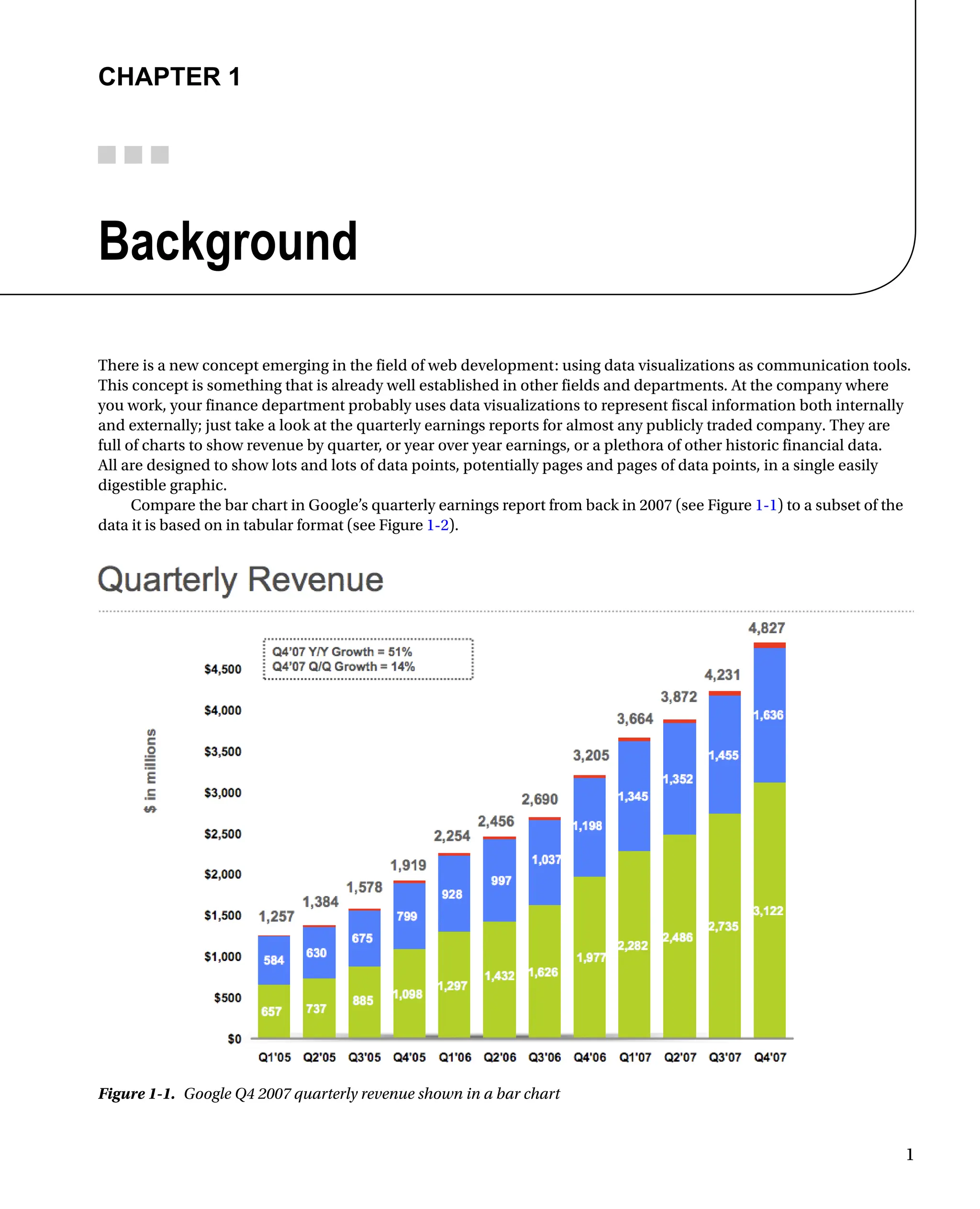
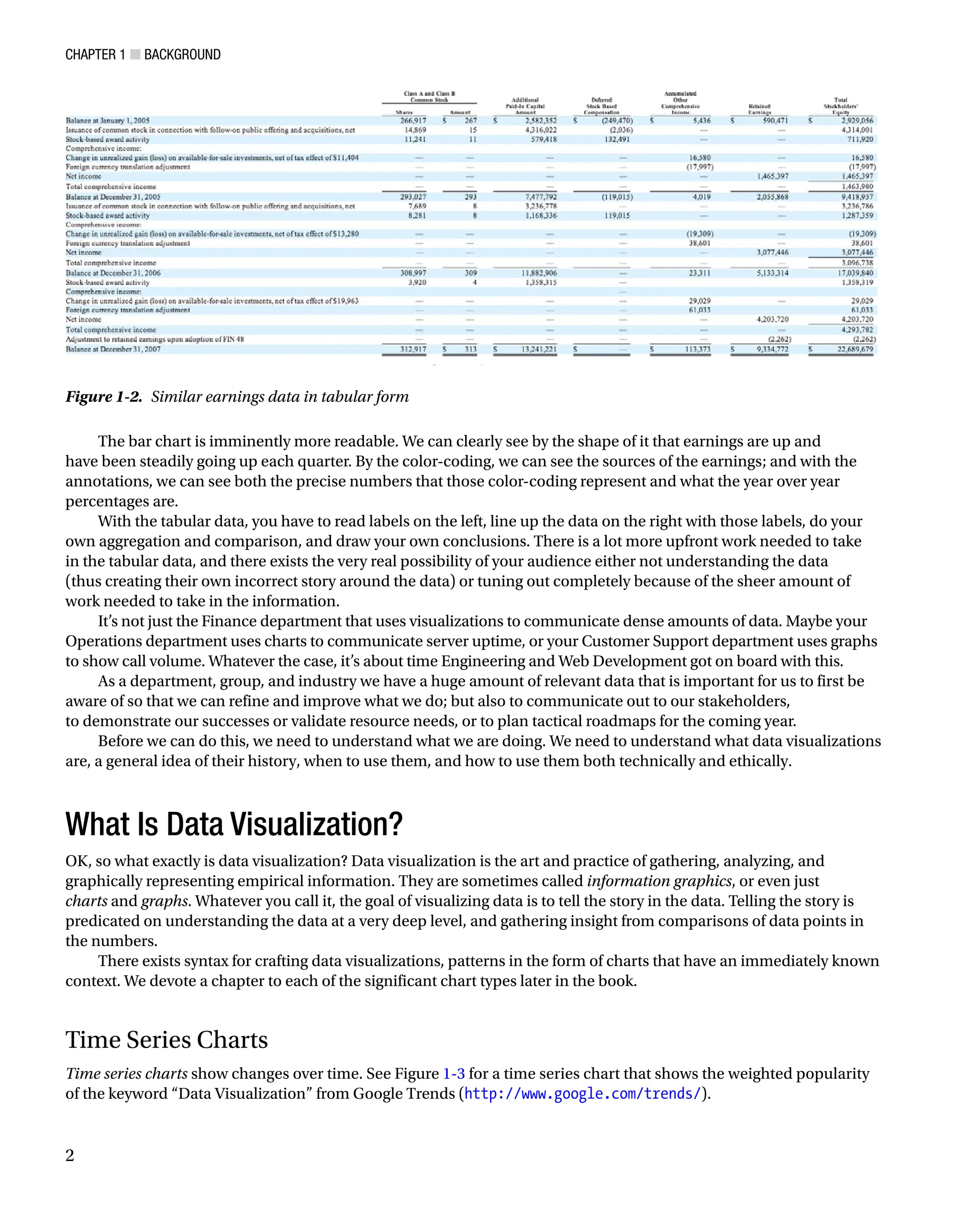
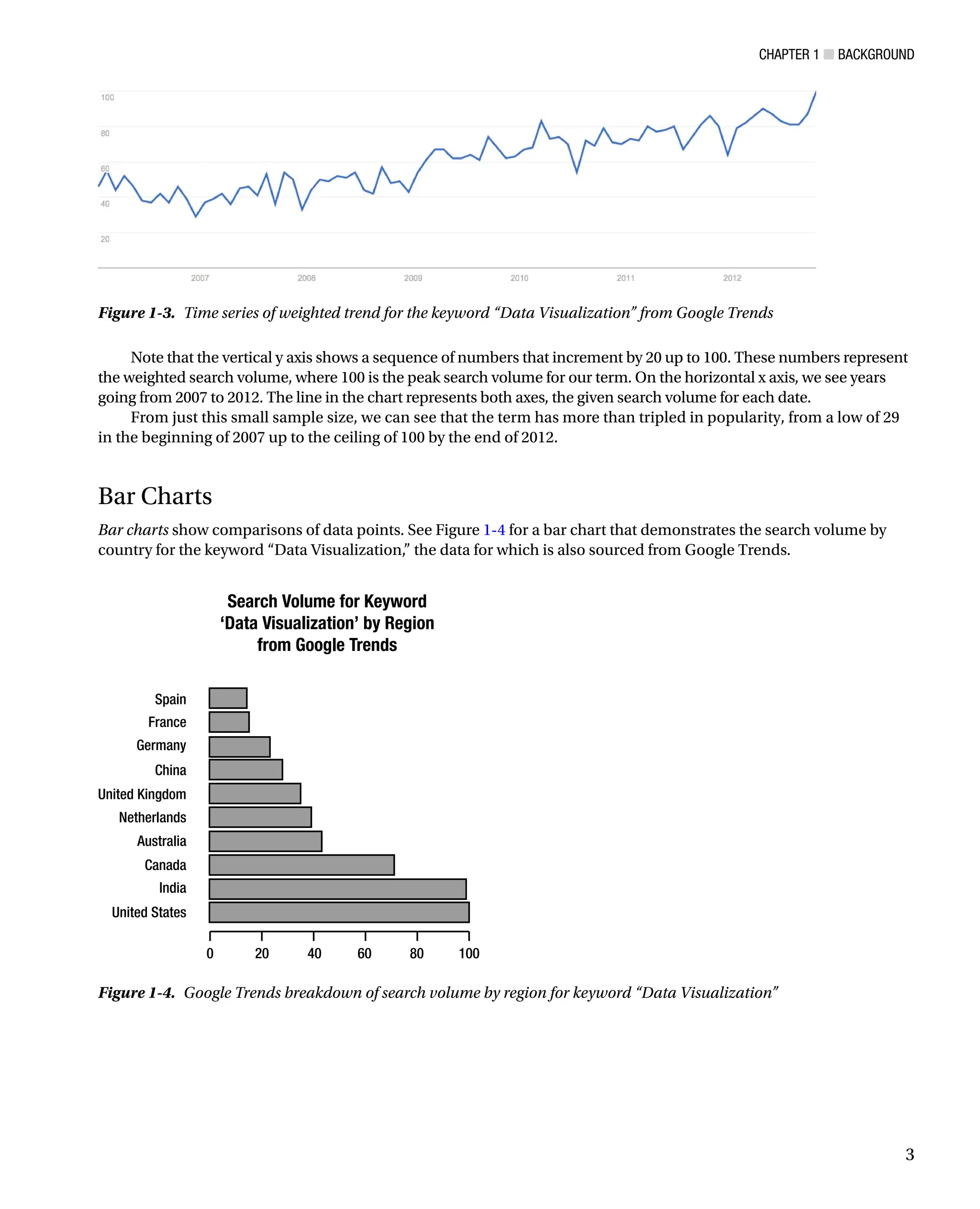
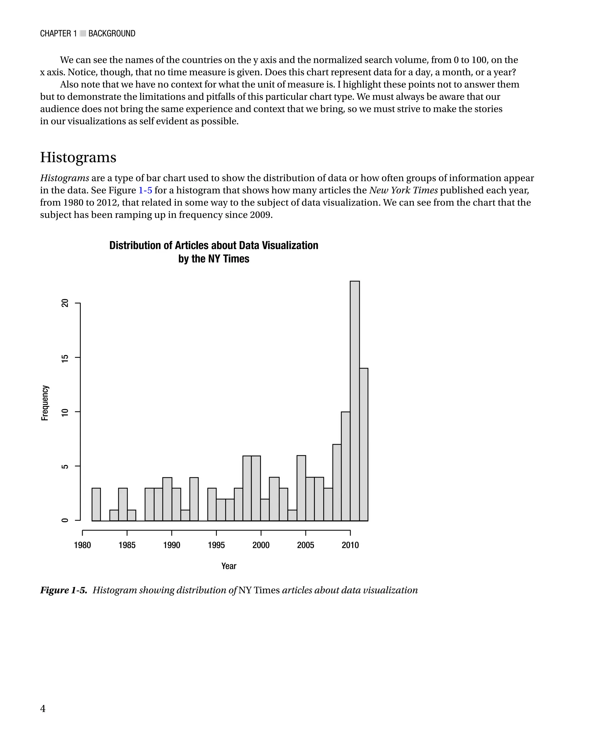
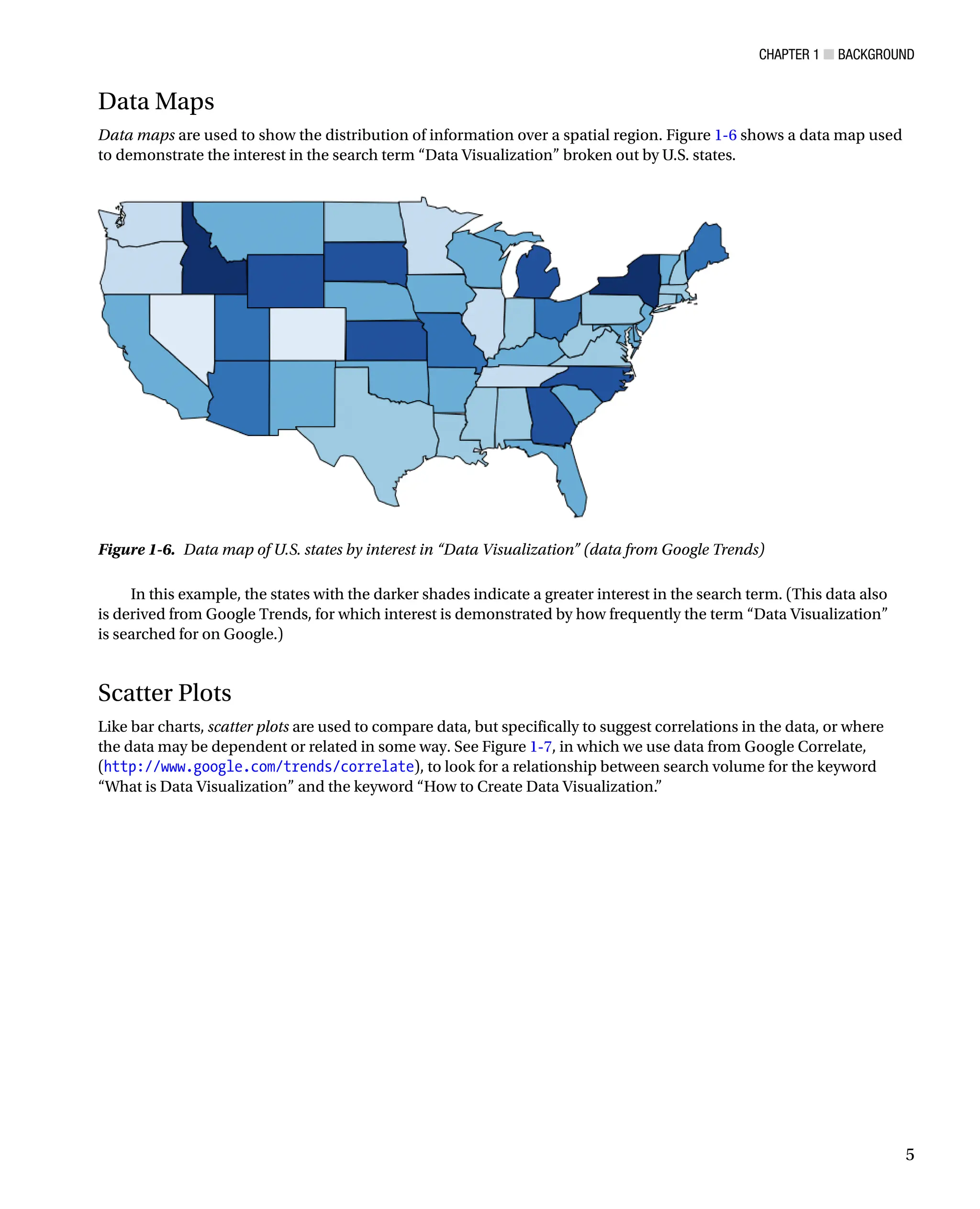
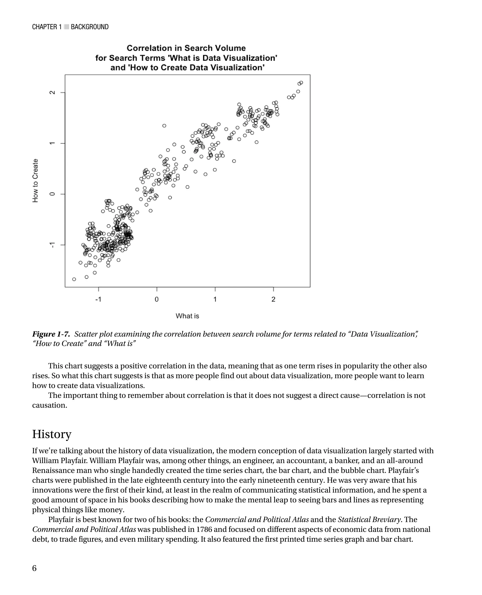

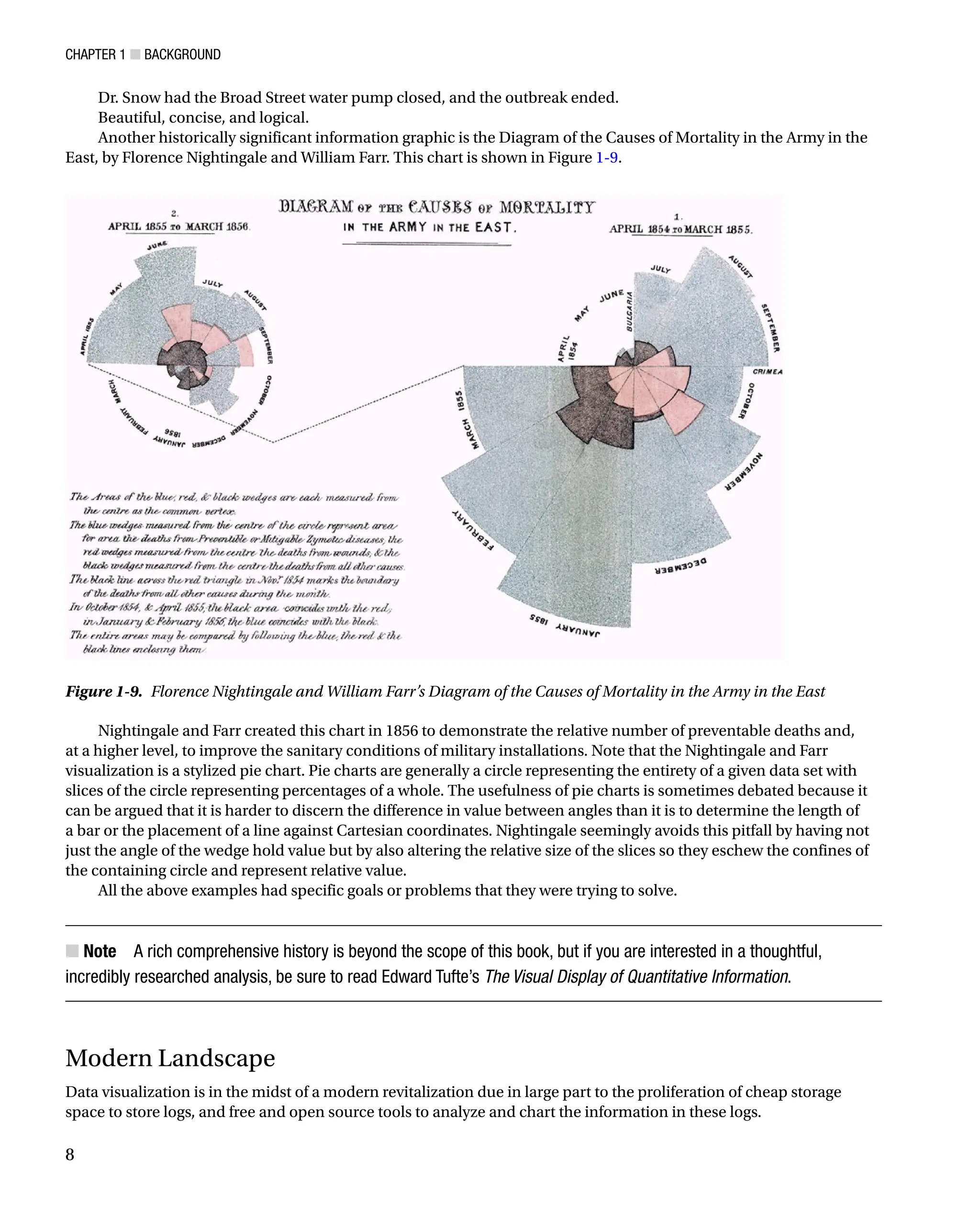
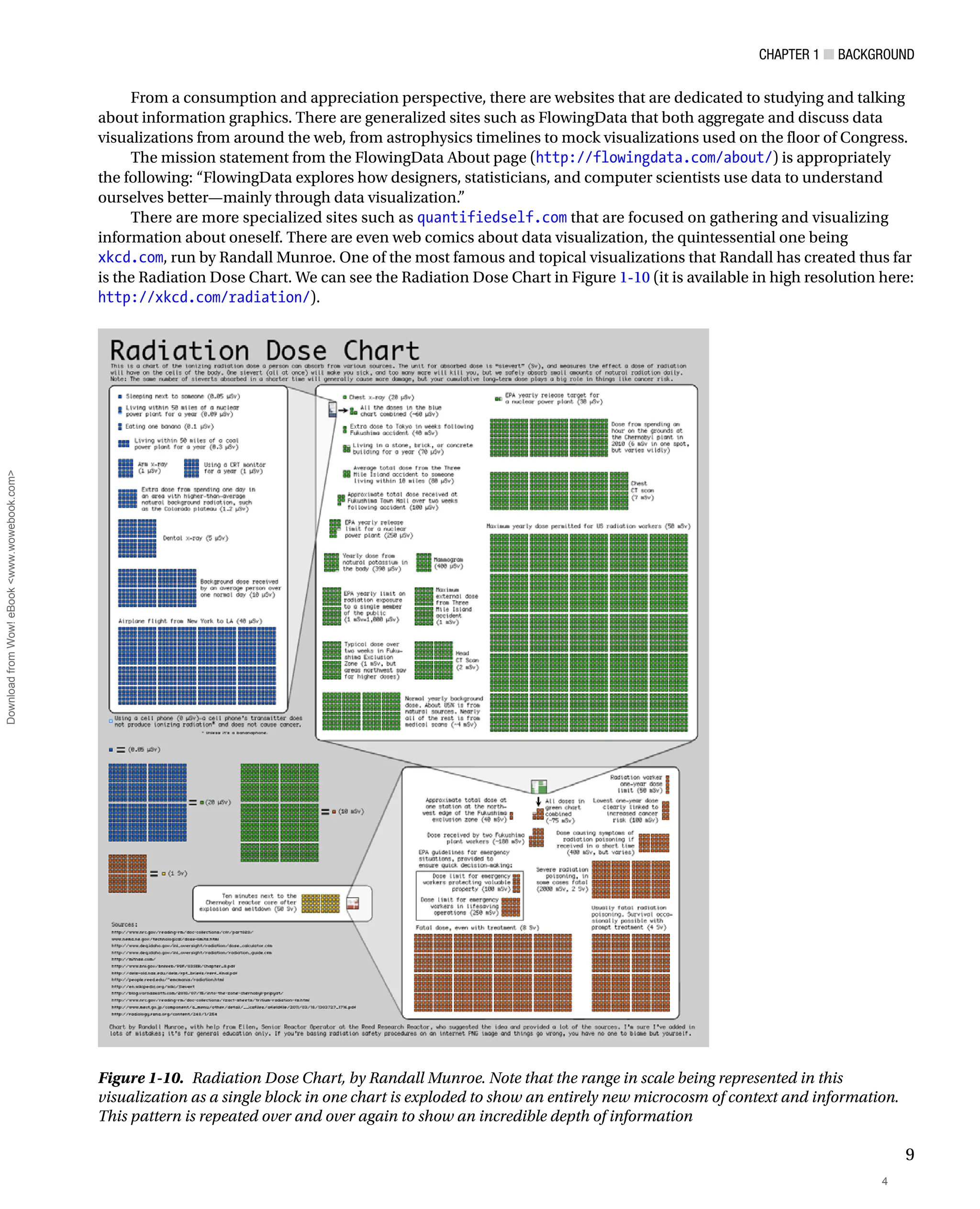
![Chapter 1 ■ Background
10
This chart was created in response to the Fukushima Daiichi nuclear disaster of 2011, and sought to clear up
misinformation and misunderstanding of comparisons being made around the disaster. It did this by demonstrating the
differences in scale for the amount of radiation from sources such as other people or a banana, up to what a fatal dose of
radiation ultimately would be—how all that compared to spending just ten minutes near the Chernobyl meltdown.
Over the last quarter of a century, Edward Tufte, author and professor emeritus at Yale University, has been
working to raise the bar of information graphics. He published groundbreaking books detailing the history of data
visualization, tracing its roots even further back than Playfair, to the beginnings of cartography. Among his principles
is the idea to maximize the amount of information included in each graphic—both by increasing the amount of
variables or data points in a chart and by eliminating the use of what he has coined chartjunk. Chartjunk, according to
Tufte, is anything included in a graph that is not information, including ornamentation or thick, gaudy arrows.
Tufte also invented the sparkline, a time series chart with all axes removed and only the trendline remaining to
show historic variations of a data point without concern for exact context. Sparklines are intended to be small enough
to place in line with a body of text, similar in size to the surrounding characters, and to show the recent or historic
trend of whatever the context of the text is.
Why Data Visualization?
In William Playfair’s introduction to the Commercial and Political Atlas, he rationalizes that just as algebra is the
abbreviated shorthand for arithmetic, so are charts a way to “abbreviate and facilitate the modes of conveying
information from one person to another.” Almost 300 years later, this principle remains the same.
Data visualizations are a universal way to present complex and varied amounts of information, as we saw in our
opening example with the quarterly earnings report. They are also powerful ways to tell a story with data.
Imagine you have your Apache logs in front of you, with thousands of lines all resembling the following:
127.0.0.1 - - [10/Dec/2012:10:39:11 +0300] GET / HTTP/1.1 200 468 - Mozilla/5.0 (X11; U;
Linux i686; en-US; rv:1.8.1.3) Gecko/20061201 Firefox/2.0.0.3 (Ubuntu-feisty)
127.0.0.1 - - [10/Dec/2012:10:39:11 +0300] GET /favicon.ico HTTP/1.1 200 766 - Mozilla/5.0
(X11; U; Linux i686; en-US; rv:1.8.1.3) Gecko/20061201 Firefox/2.0.0.3 (Ubuntu-feisty)
Among other things, we see IP address, date, requested resource, and client user agent. Now imagine this
repeated thousands of times—so many times that your eyes kind of glaze over because each line so closely resembles
the ones around it that it’s hard to discern where each line ends, let alone what cumulative trends exist within.
By using some analysis and visualization tools such as R, or even a commercial product such as Splunk, we can
artfully pull out all kinds of meaningful and interesting stories out of this log, from how often certain HTTP errors occur
and for which resources, to what our most widely used URLs are, to what the geographic distribution of our user base is.
This is just our Apache access log. Imagine casting a wider net, pulling in release information, bugs and
production incidents. What insights we could gather about what we do: from how our velocity impacts our defect
density to how our bugs are distributed across our feature sets. And what better way to communicate those findings
and tell those stories than through a universally digestible medium, like data visualizations?
The point of this book is to explore how we as developers can leverage this practice and medium as part of
continual improvement—both to identify and quantify our successes and opportunities for improvements, and more
effectively communicate our learning and our progress.
Tools
There are a number of excellent tools, environments, and libraries that we can use both to analyze and visualize our
data. The next two sections describe them.](https://image.slidesharecdn.com/5350-250227185742-8e0d2ffa/75/Pro-Data-Visualization-using-R-and-JavaScript-1st-Edition-Tom-Barker-17-2048.jpg)
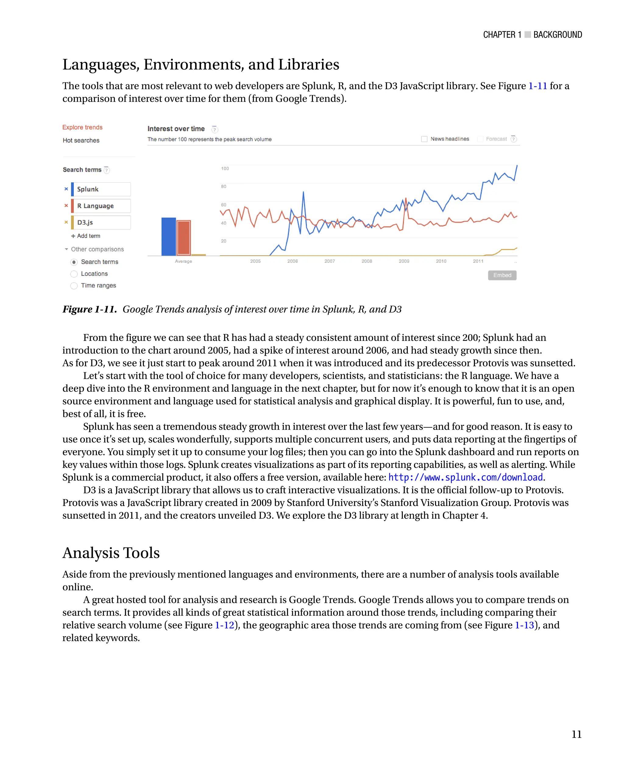
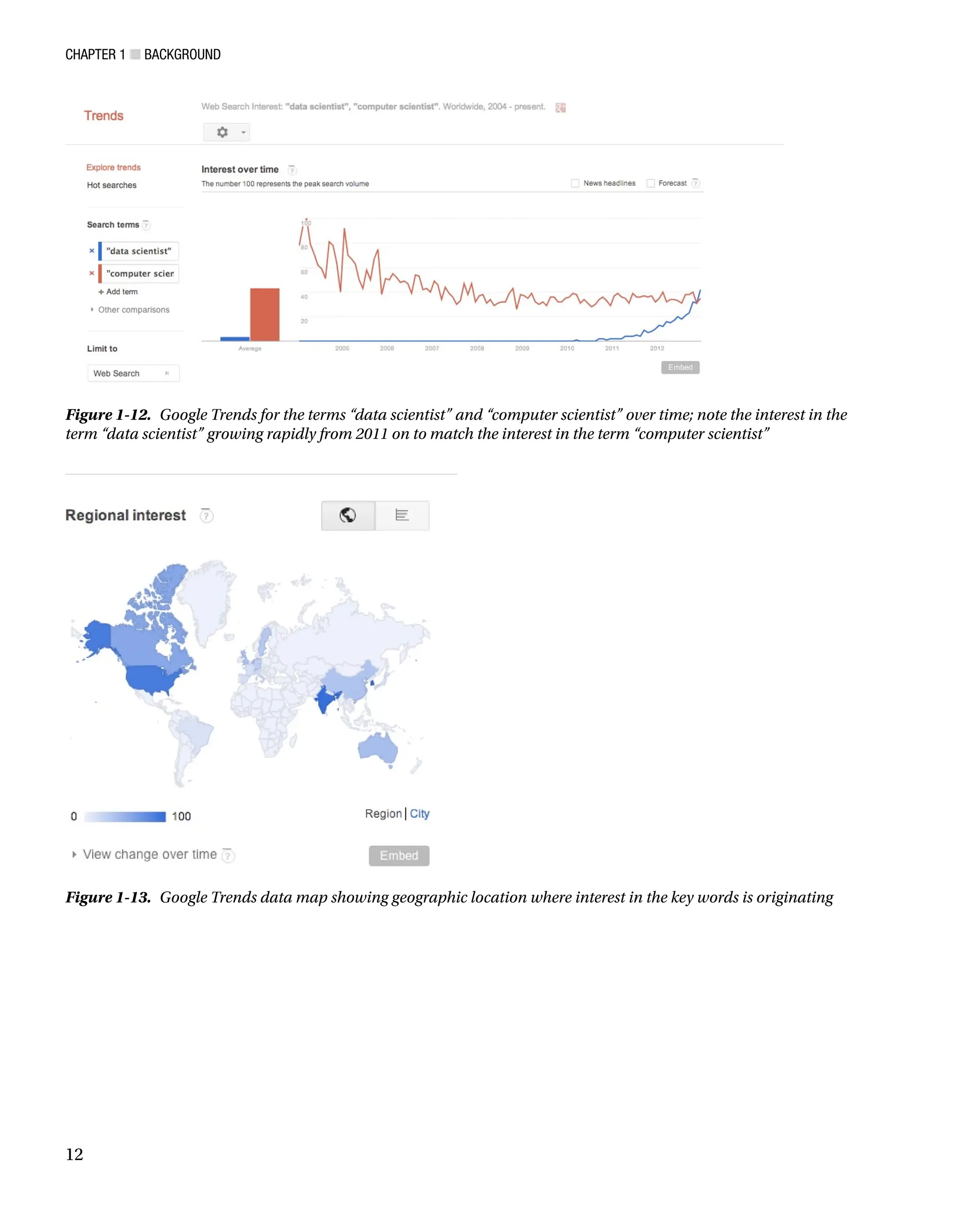

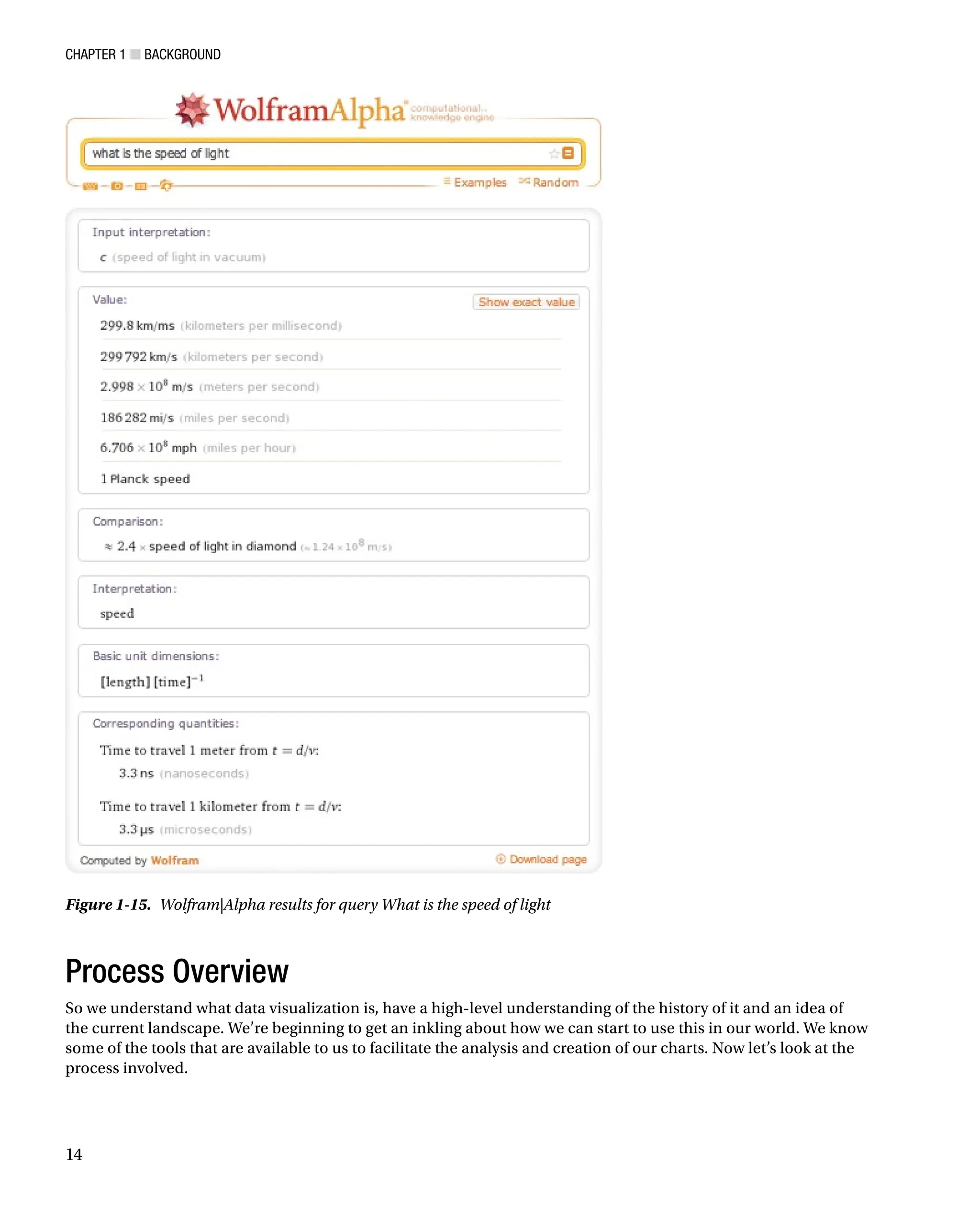
![Chapter 1 ■ Background
15
Creating data visualizations involves four core steps:
1. Identify a problem.
2. Gather the data.
3. Analyze the data.
4. Visualize the data.
Let’s walk through each step in the process and re-create one of the previous charts to demonstrate the process.
Identify a Problem
The very first step is to identify a problem we want to solve. This can be almost anything—from something as
profound and wide-reaching as figuring out why your bug backlog doesn’t seem to go down and stay down, to seeing
what feature releases over a given period in time caused the most production incidents, and why.
For our example, let’s re-create Figure 1-5 and try to quantify the interest in data visualization over time as
represented by the number of New York Times articles on the subject.
Gather Data
We have an idea of what we want to investigate, so let’s dig in. If you are trying to solve a problem or tell a story around
your own product, you would of course start with your own data—maybe your Apache logs, maybe your bug backlog,
maybe exports from your project tracking software.
Note
■
■ If you are focusing on gathering metrics around your product and you don’t already have data handy, you need to
invest in instrumentation.There are many ways to do this, usually by putting logging in your code.At the very least, you want to
log error states and monitor those, but you may want to expand the scope of what you track to include for
debugging purposes
while still respecting both your user’s privacy and your company’s privacy policy. In my book, Pro JavaScript
Performance:
Monitoring and Visualization, I explore ways to track and visualize web and runtime performance.
One important aspect of data gathering is deciding which format your data should be in (if you're lucky) or discovering
which format your data is available in. We’ll next be looking at some of the common data formats in use today.
JSON is an acronym that stands for JavaScript Object Notation. As you probably know, it is essentially a way to
send data as serialized JavaScript objects. We format JSON as follows:
[object]{
[attribute]: [value],
[method] : function(){},
[array]: [item, item]
}
Another way to transfer data is in XML format. XML has an expected syntax, in which elements can have attributes,
which have values, values are always in quotes, and every element must have a closing element. XML looks like this:
parent attribute=value
child attribute=valuenode data/child
/parent
Generally we can expect APIs to return XML or JSON to us, and our preference is usually JSON because as we can
see it is a much more lightweight option just in sheer amount of characters used.](https://image.slidesharecdn.com/5350-250227185742-8e0d2ffa/75/Pro-Data-Visualization-using-R-and-JavaScript-1st-Edition-Tom-Barker-22-2048.jpg)
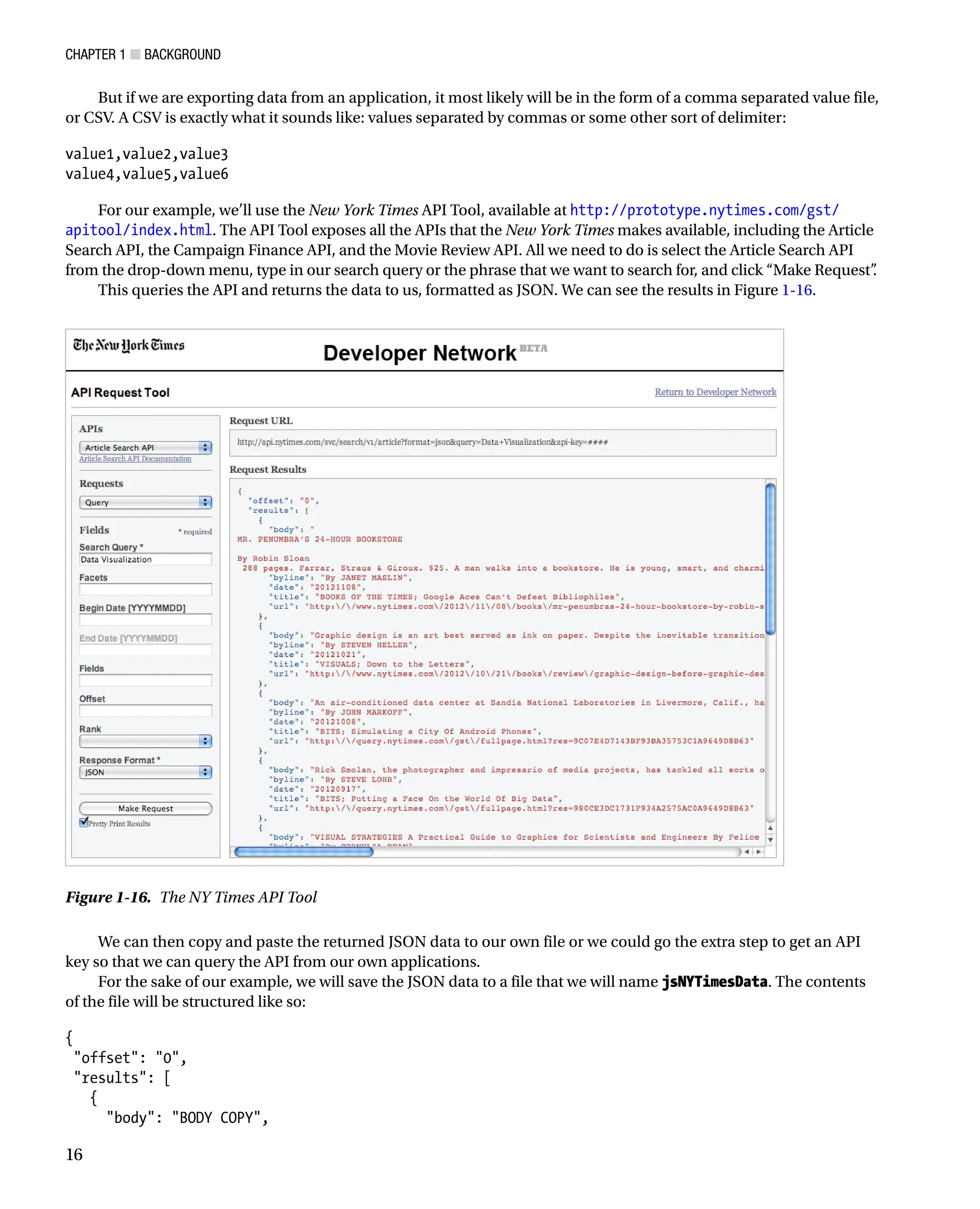
![Chapter 1 ■ Background
17
byline: By AUTHOR,
date: 20121011,
title: TITLE,
url: http://www.nytimes.com/foo.html
}, {
body: BODY COPY,
byline: By AUTHOR,
date: 20121021,
title: TITLE,
url: http://www.nytimes.com/bar.html
}
],
tokens: [
JavaScript
],
total: 2
}
Looking at the high-level JSON structure, we see an attribute named offset, an array named results, an array
named tokens, and another attribute named total. The offset variable is for pagination (what page full of results
we are starting with). The total variable is just what it sounds like: the number of results that are returned for our
query. It’s the results array that we really care about; it is an array of objects, each of which corresponds to an article.
The article objects have attributes named body, byline, date, title, and url.
We now have data that we can begin to look at. That takes us to our next step in the process, analyzing our data.
DATA SCRUBBING
There is often a hidden step here, one that anyone who’s dealt with data knows about: scrubbing the data. Often
the data is either not formatted exactly as we need it or, in even worse cases, it is dirty or incomplete.
In the best-case scenario in which your data just needs to be reformatted or even concatenated, go ahead and do
that, but be sure to not lose the integrity of the data.
Dirty data has fields out of order, fields with obviously bad information in them—think strings in ZIP codes—or
gaps in the data. If your data is dirty, you have several choices:
You could drop the rows in question, but that can harm the integrity of the data—a good example
•
is if you are creating a histogram removing rows could change the distribution and change what
your results will be.
The better alternative is to reach out to whoever administers the source of your data and try and
•
get a better version if it exists.
Whatever the case, if data is dirty or it just needs to be reformatted to be able to be imported into R, expect to
have to scrub your data at some point before you begin your analysis.
Analyze Data
Having data is great, but what does it mean? We determine it through analysis.
Analysis is the most crucial piece of creating data visualizations. It’s only through analysis that we can understand
our data, and it is only through understanding it that we can craft our story to share with others.](https://image.slidesharecdn.com/5350-250227185742-8e0d2ffa/75/Pro-Data-Visualization-using-R-and-JavaScript-1st-Edition-Tom-Barker-24-2048.jpg)
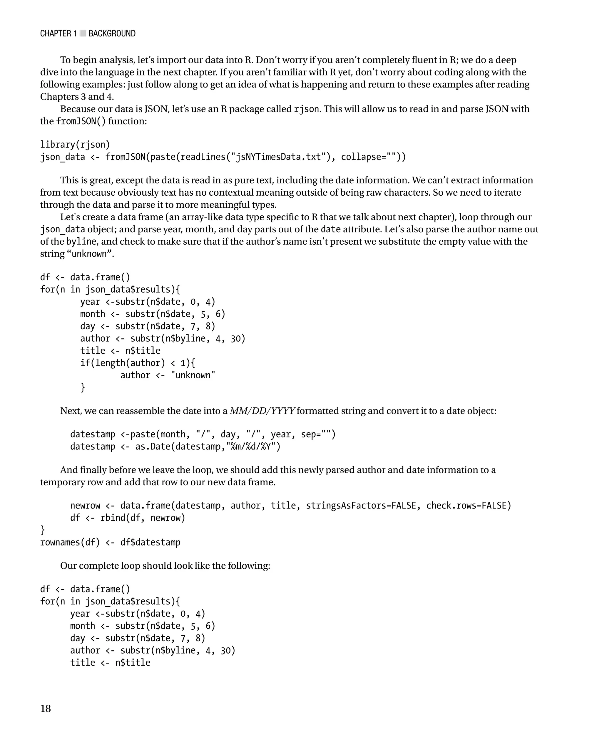
![Chapter 1 ■ BaCkground
19
if(length(author) 1){
author - unknown
}
datestamp -paste(month, /, day, /, year, sep=)
datestamp - as.Date(datestamp,%m/%d/%Y)
newrow - data.frame(datestamp, author, title, stringsAsFactors=FALSE, check.rows=FALSE)
df - rbind(df, newrow)
}
rownames(df) - df$datestamp
Note that our example assumes that the data set returned has unique date values. If you get errors with this, you
may need to scrub your returned data set to purge any duplicate rows.
Once our data frame is populated, we can start to do some analysis on the data. Let’s start out by pulling just the
year from every entry, and quickly making a stem and leaf plot to see the shape of the data.
Note John tukey created the stem and leaf plot in his seminal work, Exploratory Data Analysis. Stem and leaf plots
are quick, high-level ways to see the shape of data, much like a histogram. In the stem and leaf plot, we construct the
“stem” column on the left and the “leaf” column on the right. the stem consists of the most significant unique elements
in a result set. the leaf consists of the remainder of the values associated with each stem. In our stem and leaf plot below,
the years are our stem and r shows zeroes for each row associated with a given year. Something else to note is that
often alternating sequential rows are combined into a single row, in the interest of having a more concise visualization.
First, we will create a new variable to hold the year information:
yearlist - as.POSIXlt(df$datestamp)$year+1900
If we inspect this variable, we see that it looks something like this:
yearlist
[1] 2012 2012 2012 2012 2012 2012 2012 2012 2012 2012 2012 2012 2012 2011 2011 2011 2011 2011 2011
2011 2011 2011 2011 2011 2011 2011 2011 2011 2011
[30] 2011 2011 2011 2011 2010 2010 2010 2010 2010 2010 2010 2010 2010 2010 2009 2009 2009 2009 2009
2009 2009 2008 2008 2008 2007 2007 2007 2007 2006
[59] 2006 2006 2006 2005 2005 2005 2005 2005 2005 2004 2003 2003 2003 2002 2002 2002 2002 2001 2001
2000 2000 2000 2000 2000 2000 1999 1999 1999 1999
[88] 1999 1999 1998 1998 1998 1997 1997 1996 1996 1995 1995 1995 1993 1993 1993 1993 1992 1991 1991
1991 1990 1990 1990 1990 1989 1989 1989 1988 1988
[117] 1988 1986 1985 1985 1985 1984 1982 1982 1981
That’s great, that’s exactly what we want: a year to represent every article returned. Next let’s create the stem and
leaf plot:
stem(yearlist)
1980 | 0
1982 | 00
1984 | 0000
1986 | 0
1988 | 000000
Download
from
Wow!
eBook
www.wowebook.com](https://image.slidesharecdn.com/5350-250227185742-8e0d2ffa/75/Pro-Data-Visualization-using-R-and-JavaScript-1st-Edition-Tom-Barker-26-2048.jpg)
![Chapter 1 ■ Background
20
1990 | 0000000
1992 | 00000
1994 | 000
1996 | 0000
1998 | 000000000
2000 | 00000000
2002 | 0000000
2004 | 0000000
2006 | 00000000
2008 | 0000000000
2010 | 000000000000000000000000000000
2012 | 0000000000000
Very interesting. We see a gradual build with some dips in the mid-1990s, another gradual build with another dip
in the mid-2000s and a strong explosion since 2010 (the stem and leaf plot groups years together in twos).
Looking at that, my mind starts to envision a story building about a subject growing in popularity. But what
about the authors of these articles? Maybe they are the result of one or two very interested authors that have quite
a bit to say on the subject.
Let’s explore that idea and take a look at the author data that we parsed out. Let’s look at just the unique authors
from our data frame:
length(unique(df$author))
[1] 81
We see that there are 81 unique authors or combination of authors for these articles! Just out of curiosity, let’s take
a look at the breakdown by author for each article. Let’s quickly create a bar chart to see the overall shape of the data
(the bar chart is shown in Figure 1-17):
plot(table(df$author), axes=FALSE)
Figure 1-17. Bar chart of number of articles by author to quickly visualize](https://image.slidesharecdn.com/5350-250227185742-8e0d2ffa/75/Pro-Data-Visualization-using-R-and-JavaScript-1st-Edition-Tom-Barker-27-2048.jpg)
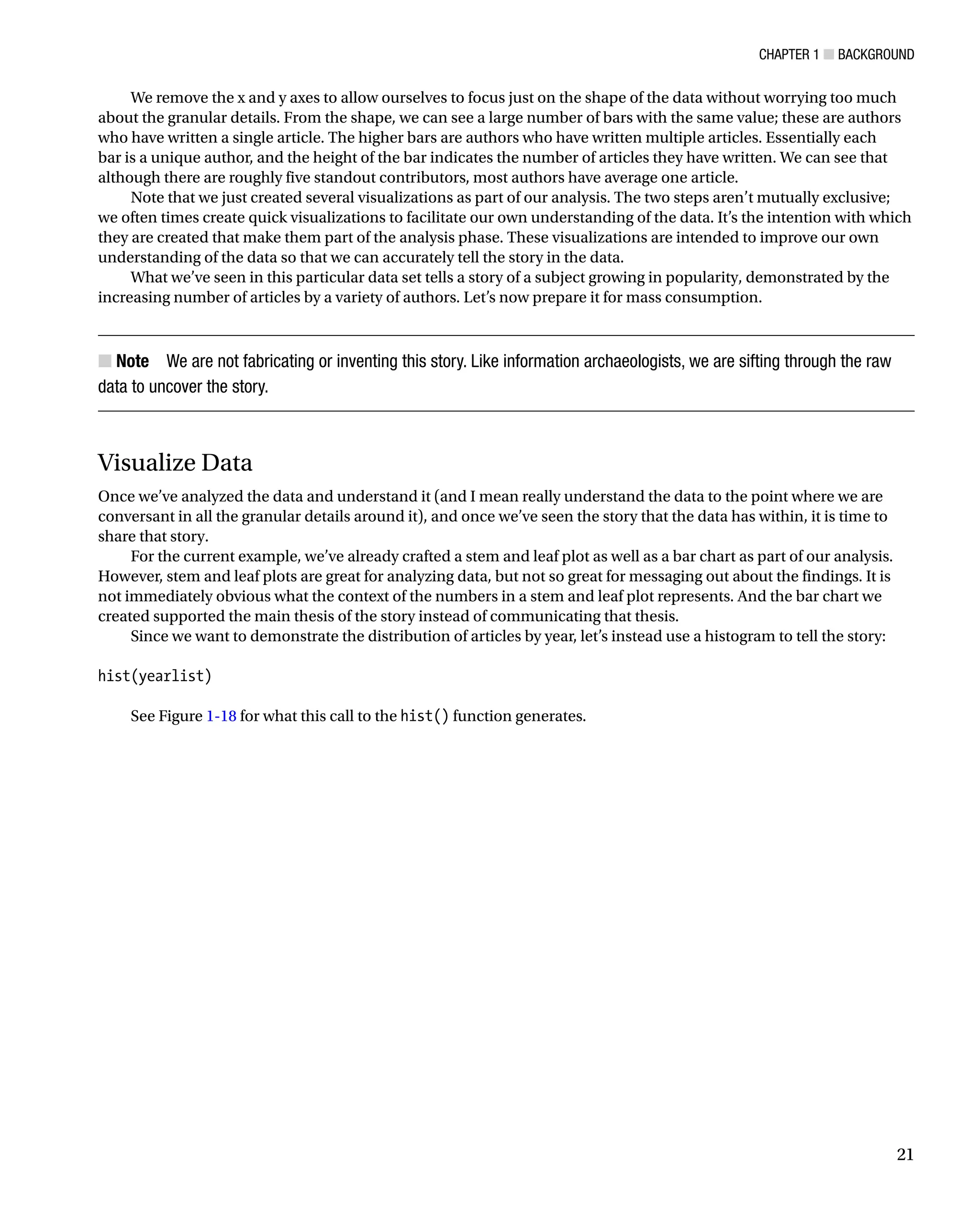
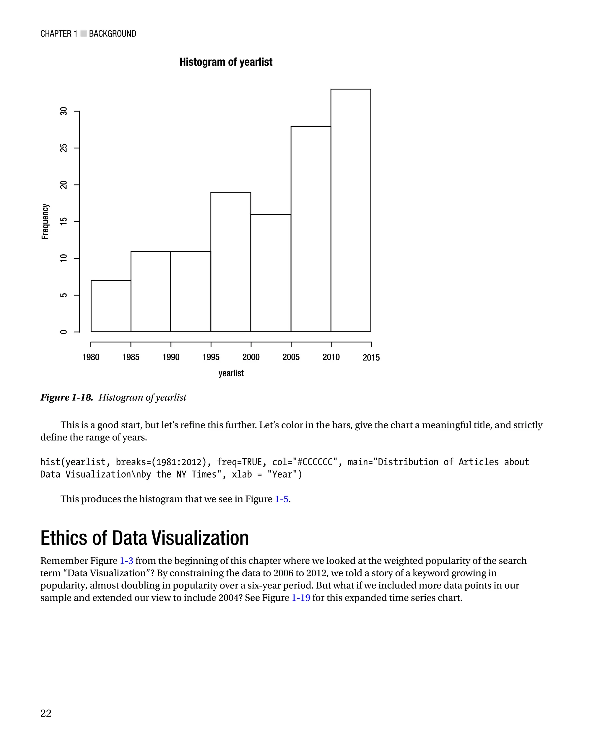
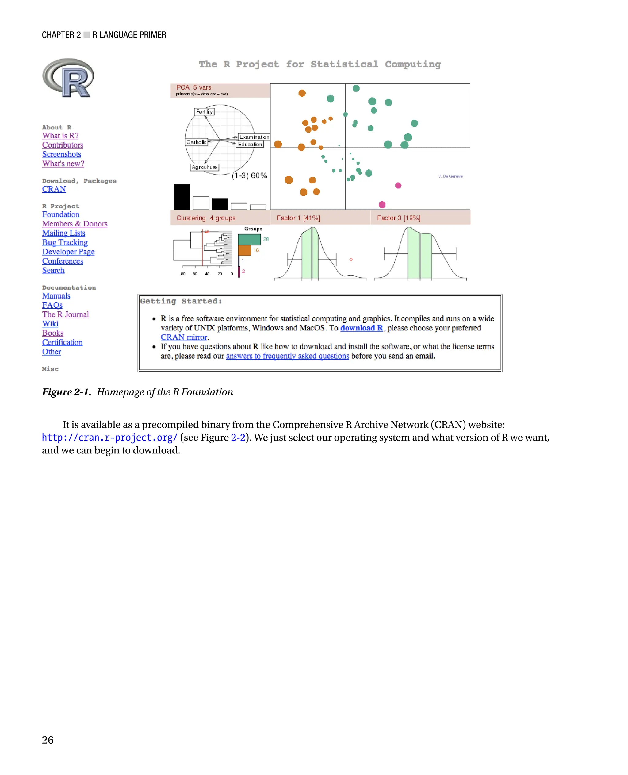
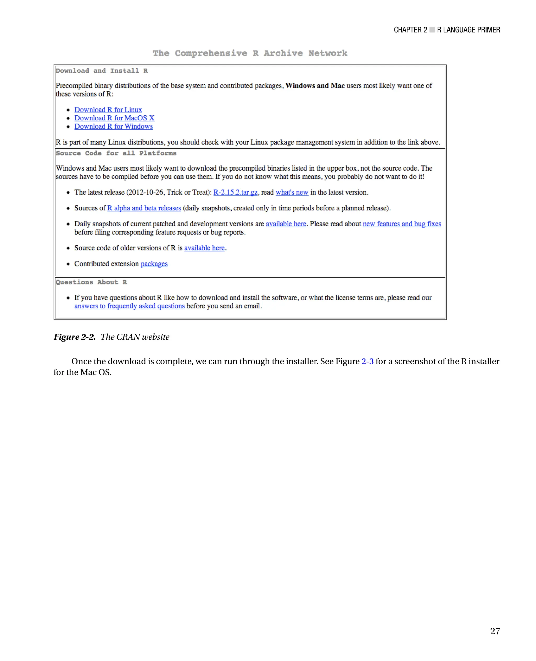
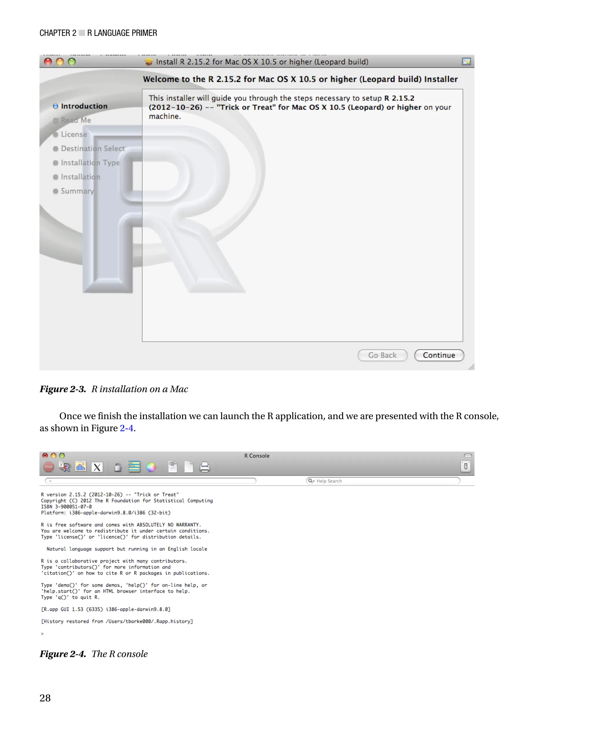
![Chapter 2 ■ R Language Primer
29
The Command Line
The R console is where the magic happens! It is a command-line environment where we can run R expressions. The best
way to get up to speed in R is to script in the console, a piece at a time, generally to try out what you’re trying to do, and
tweak it until you get the results that you want. When you finally have a working example, take the code that does what
you want and save it as an R script file.
R script files are just files that contain pure R and can be run in the console using the source command:
source(someRfile.R)
Looking at the preceding code snippet, we assume that the R script lives in the current work directory. The way
we can see what the current work directory is to use the getwd() function:
getwd()
[1] /Users/tomjbarker
We can also set the working directory by using the setwd() function. Note that changes made to the working
directory are not persisted across R sessions unless the session is saved.
setwd(/Users/tomjbarker/Downloads)
getwd()
[1] /Users/tomjbarker/Downloads
Command History
The R console stores commands that you enter and you can cycle through previous commands by pressing the up
arrow. Hit the escape button to return to the command prompt. We can see the history in a separate window pane
by clicking the Show/Hide Command History button at the top of the console. The Show/Hide Command History
button is the rectangle icon with alternating stripes of yellow and green. See Figure 2-5 for the R console with the
command history shown.](https://image.slidesharecdn.com/5350-250227185742-8e0d2ffa/75/Pro-Data-Visualization-using-R-and-JavaScript-1st-Edition-Tom-Barker-35-2048.jpg)
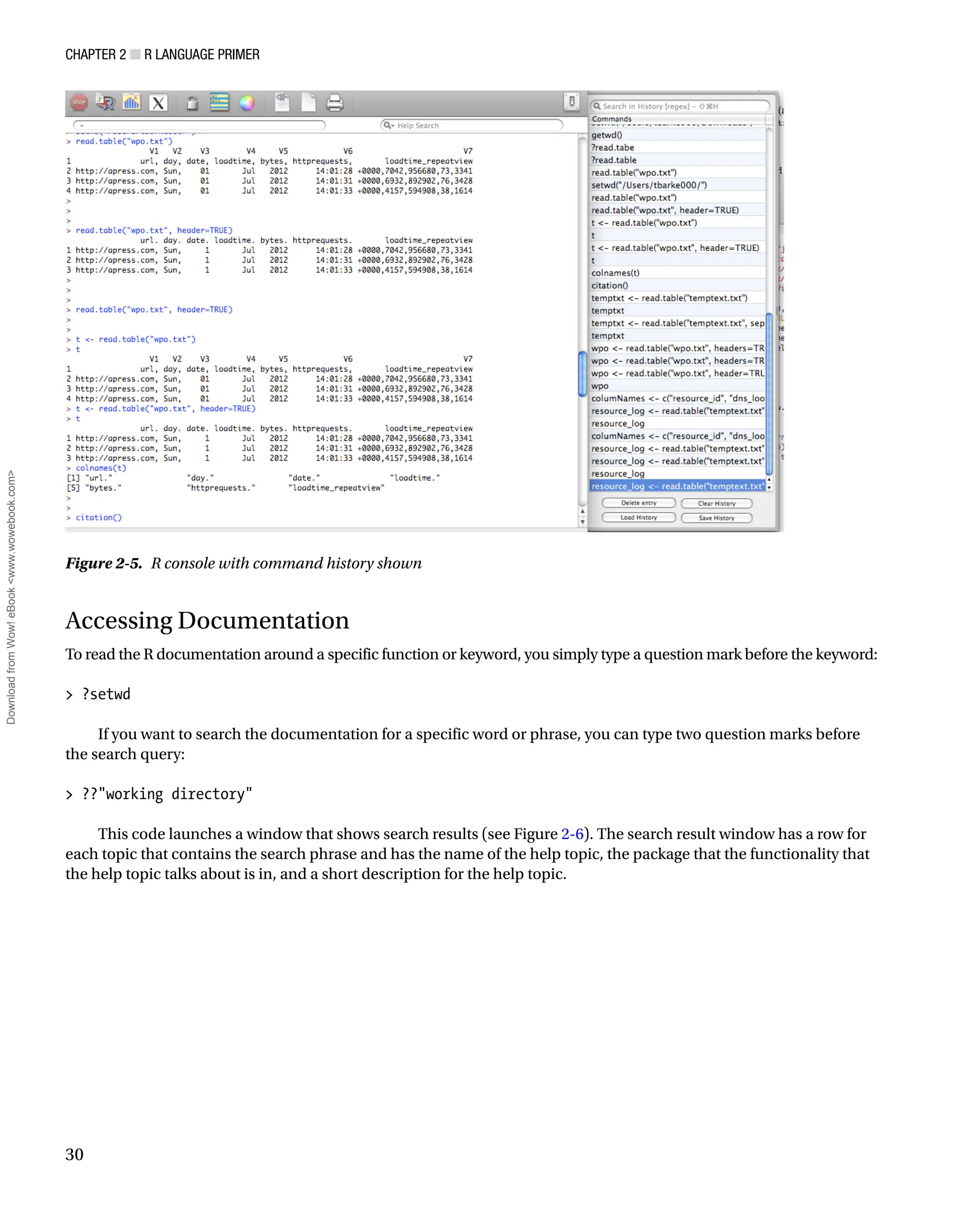
![Chapter 2 ■ R Language Primer
31
Packages
Speaking of packages, what are they, exactly? Packages are collections of functions, data sets, or objects that can
be imported into the current session or workspace to extend what we can do in R. Anyone can make a package
and distribute it.
To install a package, we simply type this:
install.packages([package name])
For example, if we want to install the ggplot2 package—which is a widely used and very handy charting
package—we simply type this into the console:
install.packages(ggplot2)
We are immediately prompted to choose the mirror location that we want to use, usually the one closest to our
current location. From there, the install begins. We can see the results in Figure 2-7.
Figure 2-6. Help search results window](https://image.slidesharecdn.com/5350-250227185742-8e0d2ffa/75/Pro-Data-Visualization-using-R-and-JavaScript-1st-Edition-Tom-Barker-37-2048.jpg)
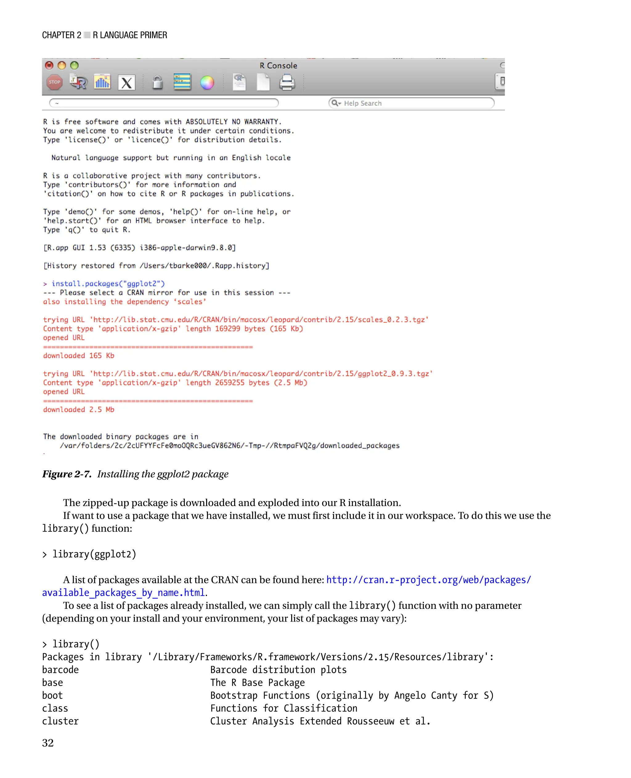
![Chapter 2 ■ R Language Primer
33
codetools Code Analysis Tools for R
colorspace Color Space Manipulation
compiler The R Compiler Package
datasets The R Datasets Package
dichromat Color schemes for dichromats
digest Create cryptographic hash digests of R objects
foreign Read Data Stored by Minitab, S, SAS, SPSS, Stata, Systat, dBase,
...
ggplot2 An implementation of the Grammar of Graphics
gpairs gpairs: The Generalized Pairs Plot
graphics The R Graphics Package
grDevices The R Graphics Devices and Support for Colours and Fonts
grid The Grid Graphics Package
gtable Arrange grobs in tables.
KernSmooth Functions for kernel smoothing for Wand Jones (1995)
labeling Axis Labeling
lattice Lattice Graphics
mapdata Extra Map Databases
mapproj Map Projections
maps Draw Geographical Maps
Importing Data
So now our environment is downloaded and installed, and we know how to install any packages that we may need.
Now we can begin using R.
The first thing we’ll normally want to do is import your data. There are several ways to import data, but the most
common way is to use the read() function, which has several flavors:
read.table([file to read])
read.csv([file to read])
To see this in action, let’s first create a text file named temptext.txt that is formatted like so:
134,432,435,313,11
403,200,500,404,33
77,321,90,2002,395
We can read this into a variable that we will name temptxt:
temptxt - read.table(temptext.txt)
Notice that as we are assigning value to this variable, we are not using an equal sign as the assignment operator.
We are instead using an arrow -. That is R’s assignment operator, although it does also support the equal sign if you
are so inclined. But the standard is the arrow, and all examples that we will show in this book will use the arrow.
If we print out the temptxt variable, we see that it is structured as follows:
temptxt
V1
1 134,432,435,313,11
2 403,200,500,404,33
3 77,321,90,2002,395](https://image.slidesharecdn.com/5350-250227185742-8e0d2ffa/75/Pro-Data-Visualization-using-R-and-JavaScript-1st-Edition-Tom-Barker-39-2048.jpg)
![Chapter 2 ■ R Language Primer
34
We see that our variable is a table-like structure called a data frame, and R has assigned a column name (V1) and
row IDs to our data structure. More on column names soon.
The read() function has a number of parameters that you can use to refine how the data is imported and
formatted once it is imported.
Using Headers
The header parameter tells R to treat the first line in the external file as containing header information. The first line
then becomes the column names of the data frame.
For example, suppose we have a log file structured like this:
url, day, date, loadtime, bytes, httprequests, loadtime_repeatview
http://apress.com, Sun, 01 Jul 2012 14:01:28 +0000,7042,956680,73,3341
http://apress.com, Sun, 01 Jul 2012 14:01:31 +0000,6932,892902,76,3428
http://apress.com, Sun, 01 Jul 2012 14:01:33 +0000,4157,594908,38,1614
We can load it into a variable named wpo like so:
wpo - read.table(wpo.txt, header=TRUE)
wpo
url day date loadtime bytes httprequests loadtime_repeatview
1 http://apress.com,Sun,1 Jul 2012 14:01:28 +0000,7042,955550,73,3191
2 http://apress.com,Sun,1 Jul 2012 14:01:31 +0000,6932,892442,76,3728
3 http://apress.com,Sun,1 Jul 2012 14:01:33 +0000,4157,614908,38,1514
When we call the colnames() function to see what the column names are for wpo, we see the following:
colnames(wpo)
[1] url day date loadtime
[5] bytes httprequests loadtime_repeatview
Specifying a String Delimiter
The sep attribute tells the read() function what to use as the string delimiter for parsing the columns in the external
data file. In all the examples we’ve looked at so far, commas are our delimiters, but we could use instead pipes | or any
other character that we want.
Say, for example, that our previous temptxt example used pipes; we would just update the code to be as follows:
134|432|435|313|11
403|200|500|404|33
77|321|90|2002|395
temptxt - read.table(temptext.txt, sep=|)
temptxt
V1 V2 V3 V4 V5
1 134 432 435 313 11
2 403 200 500 404 33
3 77 321 90 2002 395
Oh, notice that? We actually got distinct column names this time (V1, V2, V3, V4, V5). Before, we didn’t specify a
delimiter, so R assumed that each row was one big blob of text and lumped it into a single column (V1).](https://image.slidesharecdn.com/5350-250227185742-8e0d2ffa/75/Pro-Data-Visualization-using-R-and-JavaScript-1st-Edition-Tom-Barker-40-2048.jpg)
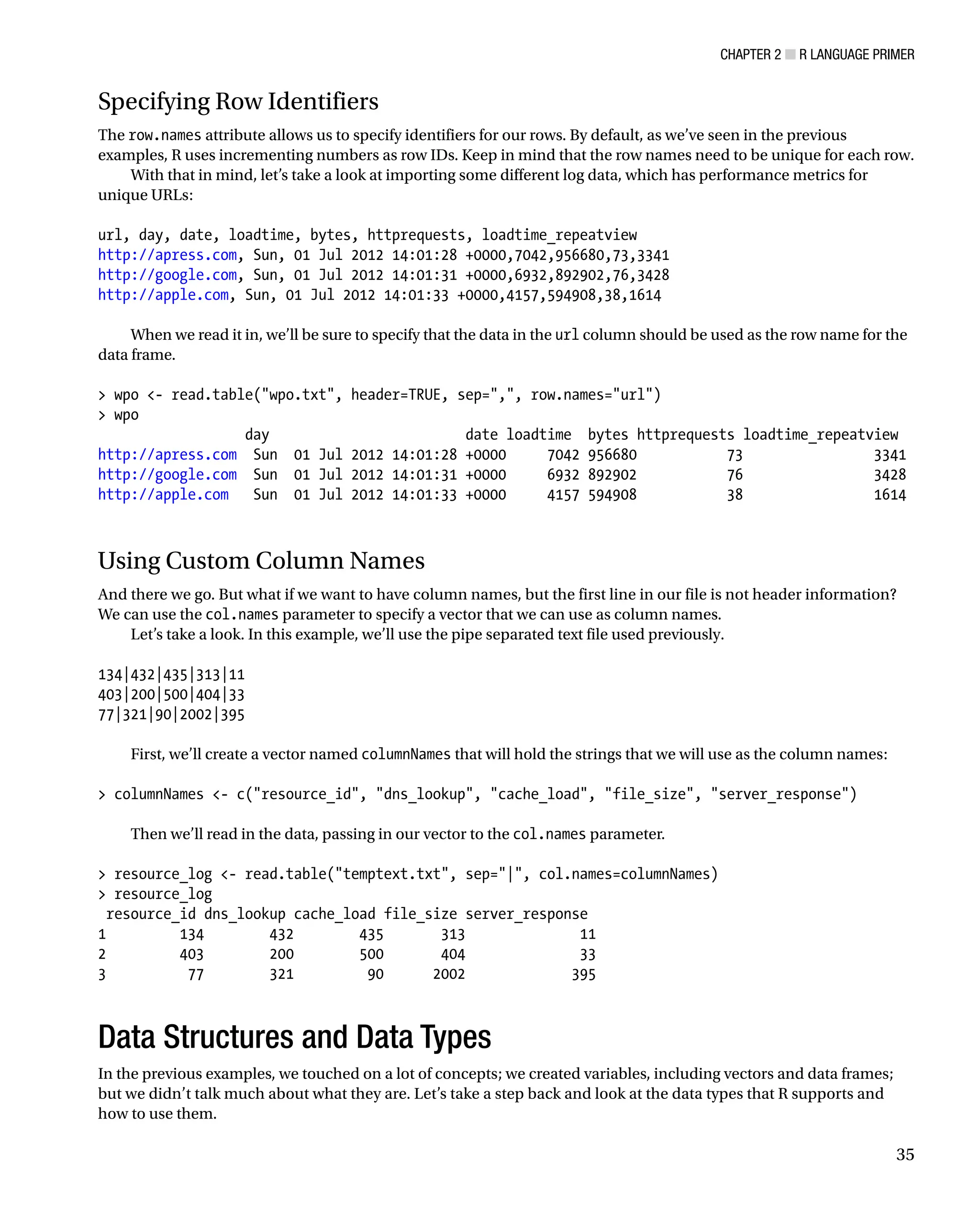
![Chapter 2 ■ R Language Primer
36
Data types in R are called modes, and can be the following:
numeric
•
character
•
logical
•
complex
•
raw
•
list
•
We can use the mode() function to check the mode of a variable.
Character and numeric modes correspond to string and number (both integer and float) data types. Logical
modes are Boolean values.
n - 122132
mode(n)
[1] numeric
c - test text
mode(c)
[1] character
l - TRUE
mode(l)
[1] logical
We can perform string concatenation using the paste() function. We can use the substr() function to pull
characters out of strings. Let’s look at some examples in code.
Usually, I keep a list of directories that I either read data from or write charts to. Then when I want to reference
a new data file that exists in the data directory, I will just append the new file name to the data directory:
dataDirectory - /Users/tomjbarker/org/data/
buglist - paste(dataDirectory, bugs.txt, sep=)
buglist
[1] /Users/tomjbarker/org/data/bugs.txt
The paste() function takes N amount of strings and concatenates them together. It accepts an argument named
sep that allows us to specify a string that we can use to be a delimiter between joined strings. We don’t want anything
separating our joined strings that we pass in an empty string.
If we want to pull characters from a string, we use the substr() function. The substr() function takes a string to
parse, a starting location, and a stopping location. It returns all the character inclusively from the starting location up
to the ending location. (Remember that in R, lists are not 0-based like most other languages, but instead have
a starting index of 1.)
substr(test, 1,2)
[1] te
In the preceding example, we pass in the string “test” and tell the substr() function to return the first and
second characters.
Complex mode is for complex numbers. The raw mode is to store raw byte data.](https://image.slidesharecdn.com/5350-250227185742-8e0d2ffa/75/Pro-Data-Visualization-using-R-and-JavaScript-1st-Edition-Tom-Barker-42-2048.jpg)
![Chapter 2 ■ R Language Primer
37
List data types or modes can be one of three classes: vectors, matrices, or data frames. If we call mode() for vectors
or matrices, they return the mode of the data that they contain; class() returns the class. If we call mode() on a data
frame, it returns the type list:
v - c(1:10)
mode(v)
[1] numeric
m - matrix(c(1:10), byrow=TRUE)
mode(m)
[1] numeric
class(m)
[1] matrix
d - data.frame(c(1:10))
mode(d)
[1] list
class(d)
[1] data.frame
Note that we just typed 1:10 rather than the whole sequence of numbers between 1 and 10:
v - c(1:10)
Vectors are single-dimensional arrays that can hold only values of a single mode at a time. It’s when we get to
data frames and matrices that R really starts to get interesting. The next two sections cover those classes.
Data Frames
We saw at the beginning of this chapter that the read() function takes in external data and saves it as a data frame.
Data frames are like arrays in most other loosely typed languages: they are containers that hold different types of data,
referenced by index. The main thing to realize, though, is that data frames see the data that they contain as rows, columns,
and combinations of the two.
For example, think of a data frame as formatted as follows:
col col col col col
row [ 1 ] [ 1 ] [ 1 ] [ 1 ] [ 1 ]
row [ 1 ] [ 1 ] [ 1 ] [ 1 ] [ 1 ]
row [ 1 ] [ 1 ] [ 1 ] [ 1 ] [ 1 ]
row [ 1 ] [ 1 ] [ 1 ] [ 1 ] [ 1 ]
If we try to reference the first index in the preceding data frame as we traditionally would with an array, say
dataframe[1], R would instead return the first column of data, not the first item. So data frames are referenced by their
column and row. So dataframe[1] returns the first column and dataframe[,2] returns the first row.
Let’s demonstrate this in code.
First let’s create some vectors using the combine function, c(). Remember that vectors are collections of data all
of the same type. The combine function takes a series of values and combines them into vectors.
col1 - c(1,2,3,4,5,6,7,8)
col2 - c(1,2,3,4,5,6,7,8)
col3 - c(1,2,3,4,5,6,7,8)
col4 - c(1,2,3,4,5,6,7,8)](https://image.slidesharecdn.com/5350-250227185742-8e0d2ffa/75/Pro-Data-Visualization-using-R-and-JavaScript-1st-Edition-Tom-Barker-43-2048.jpg)
![Chapter 2 ■ R Language Primer
38
Then let’s combine these vectors into a data frame:
df - data.frame(col1,col2,col3,col4)
Now let’s print the data frame to see the contents and the structure of it:
df
col1 col2 col3 col4
1 1 1 1 1
2 2 2 2 2
3 3 3 3 3
4 4 4 4 4
5 5 5 5 5
6 6 6 6 6
7 7 7 7 7
8 8 8 8 8
Notice that it took each vector and made each one a column. Also notice that each row has an ID; by default,
it is a number, but we can override that.
If we reference the first index, we see that the data frame returns the first column:
df[1]
col1
1 1
2 2
3 3
4 4
5 5
6 6
7 7
8 8
If we put a comma in front of that 1, we reference the first row:
df[,1]
[1] 1 2 3 4 5 6 7 8
So accessing contents of a data frame is done by specifying [column, row].
Matrices work much the same way.
Matrices
Matrices are just like data frames in that they contain rows and columns and can be referenced by either. The core
difference between the two is that data frames can hold different data types but matrices can hold only one type of data.
This presents a philosophical difference. Usually you use data frames to hold data read in externally, like from a
flat file or a database because those are generally of mixed type. You normally store data in matrices that you want to
apply functions to (more on applying functions to lists in a little bit).](https://image.slidesharecdn.com/5350-250227185742-8e0d2ffa/75/Pro-Data-Visualization-using-R-and-JavaScript-1st-Edition-Tom-Barker-44-2048.jpg)
![Chapter 2 ■ R Language Primer
39
To create a matrix, we must use the matrix() function, pass in a vector, and tell the function how to distribute
the vector:
The
• nrow parameter specifies how many rows the matrix should have
The
• ncol parameter specifies the number of columns.
The
• byrow parameter tells R that the contents of the vector should be distributed by iterating
across rows if TRUE or by columns if FALSE.
content - c(1,2,3,4,5,6,7,8,9,10)
m1 - matrix(content, nrow=2, ncol=5, byrow=TRUE)
m1
[,1] [,2] [,3] [,4] [,5]
[1,] 1 2 3 4 5
[2,] 6 7 8 9 10
Notice that in the previous example that the m1 matrix is filled in horizontally, row by row. In the following
example, the m1 matrix is filled in vertically by column:
content - c(1,2,3,4,5,6,7,8,9,10)
m1 - matrix(content, nrow=2, ncol=5, byrow=FALSE)
m1
[,1] [,2] [,3] [,4] [,5]
[1,] 1 3 5 7 9
[2,] 2 4 6 8 10
Remember that instead of manually typing out all the numbers in the previous content vector, if the numbers are
a sequence we can just type this:
content - (1:10)
We reference the content in matrices with the square bracket, specifying the row and column, respectively.
m1[1,4]
[1] 7
We can convert a data frame to a matrix if the data frame contains only a single type of data. To do this we use the
as.matrix() function. Often times we will do this when passing a data frame to a plotting function to draw a chart.
barplot(as.matrix(df))
Below we create a data frame called df. We populate the data frame with ten consecutive numbers. We then use
as.matrix() to convert df into a matrix and save the result into a new variable called m:
df - data.frame(1:10)
df
X1.10
1 1
2 2
3 3](https://image.slidesharecdn.com/5350-250227185742-8e0d2ffa/75/Pro-Data-Visualization-using-R-and-JavaScript-1st-Edition-Tom-Barker-45-2048.jpg)
![Chapter 2 ■ r Language primer
40
4 4
5 5
6 6
7 7
8 8
9 9
10 10
class(df)
[1] data.frame
m - as.matrix(df)
class(m)
[1] matrix
Keep in mind that because they are all the same data type, matrices require less overhead and are intrinsically
more efficient than data frames. If we compare the size of our matrix m and our data frame df, we see that with just ten
items there is a size difference.
object.size(m)
312 bytes
object.size(df)
440 bytes
With that said, if we increase the scale of this, the increase in efficiency does not equally scale. Compare the following:
big_df - data.frame(1:40000000)
big_m - matrix(1:40000000)
object.size(big_m)
160000112 bytes
object.size(big_df)
160000400 bytes
We can see that the first example with the small data set showed that the matrix was 30 percent smaller in size
than the data frame, but at the larger scale in the second example the matrix was only .00018 percent smaller than
the data frame.
Adding Lists
When combining or adding to data frames or matrices, you generally add either by the row or the column using
rbind() or cbind().
To demonstrate this, let’s add a new row to our data frame df. We’ll pass df into rbind() along with the new row
to add to df. The new row contains just one element, the number 11:
df - rbind(df, 11)
df
X1.10
1 1
2 2
3 3
4 4
5 5
6 6
Download
from
Wow!
eBook
www.wowebook.com](https://image.slidesharecdn.com/5350-250227185742-8e0d2ffa/75/Pro-Data-Visualization-using-R-and-JavaScript-1st-Edition-Tom-Barker-46-2048.jpg)
![Chapter 2 ■ R Language Primer
41
7 7
8 8
9 9
10 10
11 11
Now let’s add a new column to our matrix m. To do this, we simply pass m into cbind() as the first parameter;
the second parameter is a new matrix that will be appended to the new column.
m - rbind(m, 11)
m - cbind(m, matrix(c(50:60), byrow=FALSE))
m
X1.10
[1,] 1 50
[2,] 2 51
[3,] 3 52
[4,] 4 53
[5,] 5 54
[6,] 6 55
[7,] 7 56
[8,] 8 57
[9,] 9 58
[10,] 10 59
[11,] 11 60
What about vectors, you may ask? Well, let’s look at adding to our content vector. We simply use the combine
function to combine the current vector with a new vector:
content - c(1,2,3,4,5,6,7,8,9,10)
content - c(content, c(11:20))
content
[1] 1 2 3 4 5 6 7 8 9 10 11 12 13 14 15 16 17 18 19 20
Looping Through Lists
As developers who generally work in procedural languages, or at least came up the ranks using procedural languages
(though in recent years functional programming paradigms have become much more mainstream), we’re most
likely used to looping through our arrays when we want to process the data within them. This is in contrast to purely
functional languages where we would instead apply a function to our lists, like the map() function. R supports both
paradigms. Let’s first look at how to loop through our lists.
The most useful loop that R supports is the for in loop. The basic structure of a for in loop can be seen here:.
for(i in 1:5){print(i)}
[1] 1
[1] 2
[1] 3
[1] 4
[1] 5](https://image.slidesharecdn.com/5350-250227185742-8e0d2ffa/75/Pro-Data-Visualization-using-R-and-JavaScript-1st-Edition-Tom-Barker-47-2048.jpg)
![Chapter 2 ■ R Language Primer
42
The variable i increments in value each step through the iteration. We can use the for in loop to step through
lists. We can specify a particular column to iterate through, like the following, in which we loop through the X1.10
column of the data frame df.
for(n in df$X1.10){ print(n)}
[1] 1
[1] 2
[1] 3
[1] 4
[1] 5
[1] 6
[1] 7
[1] 8
[1] 9
[1] 10
[1] 11
Note that we are accessing the columns of data frames via the dollar sign operator. The general pattern is
[data frame]$[column name].
Applying Functions to Lists
But the way that R really wants to be used is to apply functions to the contents of lists (see Figure 2-8).
function
element
element
element
element
Figure 2-8. Apply a function to list elements
We do this in R with the apply() function.](https://image.slidesharecdn.com/5350-250227185742-8e0d2ffa/75/Pro-Data-Visualization-using-R-and-JavaScript-1st-Edition-Tom-Barker-48-2048.jpg)
![Chapter 2 ■ R Language Primer
43
The apply() function takes several parameters:
First is our list.
•
Next a number vector to indicate how we apply the function through the list (
• 1 is for rows, 2 is
for columns, and c[1,2] indicates both rows and columns).
Finally is the function to apply to the list:
•
apply([list], [how to apply function], [function to apply])
Let’s look at an example. Let’s make a new matrix that we’ll call m. The matrix m will have ten columns and four rows:
m - matrix(c(1:40), byrow=FALSE, ncol=10)
m
[,1] [,2] [,3] [,4] [,5] [,6] [,7] [,8] [,9] [,10]
[1,] 1 5 9 13 17 21 25 29 33 37
[2,] 2 6 10 14 18 22 26 30 34 38
[3,] 3 7 11 15 19 23 27 31 35 39
[4,] 4 8 12 16 20 24 28 32 36 40
Now say we wanted to increment every number in the m matrix. We could simply use apply() as follows:
apply(m, 2, function(x) x - x + 1)
[,1] [,2] [,3] [,4] [,5] [,6] [,7] [,8] [,9] [,10]
[1,] 2 6 10 14 18 22 26 30 34 38
[2,] 3 7 11 15 19 23 27 31 35 39
[3,] 4 8 12 16 20 24 28 32 36 40
[4,] 5 9 13 17 21 25 29 33 37 41
Do you see what we did there? We passed in m, we specified that we wanted to apply the function across the
columns, and finally we passed in an anonymous function. The function accepts a parameter that we called x.
The parameter x is a reference to the current matrix element. From there, we just increment the value of x by 1.
OK, say we wanted to do something slightly more interesting, such as zeroing out all the even numbers in the
matrix. We could do the following:
apply(m,c(1,2),function(x){if((x %% 2) == 0) x - 0 else x - x})
[,1] [,2] [,3] [,4] [,5] [,6] [,7] [,8] [,9] [,10]
[1,] 1 5 9 13 17 21 25 29 33 37
[2,] 0 0 0 0 0 0 0 0 0 0
[3,] 3 7 11 15 19 23 27 31 35 39
[4,] 0 0 0 0 0 0 0 0 0 0
For the sake of clarity let’s break out that function that we are applying. We simply check to see whether the
current element is even by checking to see whether it has a remainder when divided by two. If it is, we set it to zero;
if it isn’t, we set it to itself:
function(x){
if((x %% 2) == 0)
x - 0
else
x - x
}](https://image.slidesharecdn.com/5350-250227185742-8e0d2ffa/75/Pro-Data-Visualization-using-R-and-JavaScript-1st-Edition-Tom-Barker-49-2048.jpg)

{
[body of function]
}
Something interesting that R allows is the ... argument (sometimes called the dots argument). This allows us to
pass in a variable number of parameters into a function. Within the function, we can convert the ... argument into a list
and iterate over the list to retrieve the values within:
offset - function (...){
for(i in list(...)){
print(i)
}
}
offset(23,11)
[1] 23
[1] 11
We can even store values of different data types (modes) in the ... argument:
offset(test value, 12, 100, 19ANM)
[1] test value
[1] 12
[1] 100
[1] 19ANM
R uses lexical scoping. This means that when we call a function and try to reference variables that are not defined
inside the local scope of the function, the R interpreter looks for those variables in the workspace or scope in which the
function was created. If the R interpreter cannot find those variables in that scope, it looks in the parent of that scope.
If we create a function A within function B, the creation scope of function A is function B. For example, see the
following code snippet:
x - 10
wrapper - function(y){
x - 99
c- function(y){
print(x + y)
}
return(c)
}
t - wrapper()
t(1)
[1] 100
x
[1] 10](https://image.slidesharecdn.com/5350-250227185742-8e0d2ffa/75/Pro-Data-Visualization-using-R-and-JavaScript-1st-Edition-Tom-Barker-50-2048.jpg)
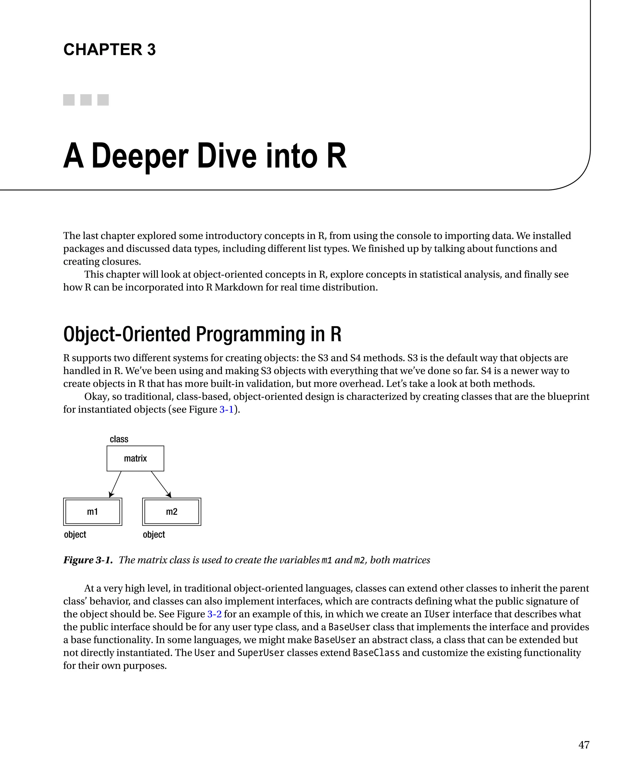
![Chapter 3 ■ A Deeper Dive into R
48
There also exists the concept of polymorphism, in which we can change functionality via the inheritance chain.
Specifically, we would inherit a function from a base class but override it, keep the signature (the function name, the
type and amount of parameters it accepts, and the type of data that it returns) the same, but change what the function
does. Compare overriding a function to the contrasting concept of overloading a function, in which the function
would have the same name but a different signature and functionality.
S3 Classes
S3, so called because it was first implemented in version 3 of the S language, uses a concept called generic functions.
Everything in R is an object, and each object has a string property called class that signifies what the object is. There
is no validation around it, and we can overwrite the class property ad hoc. That’s the main problem with S3—the
lack of validation. If you ever had an esoteric error message returned when trying to use a function, you probably
experienced the repercussions of this lack of validation firsthand. The error message was probably generated not from
R detecting that an incorrect type had been passed in, but from the function trying to execute with what was passed in
and failing at some step along the way.
See the following code, in which we create a matrix and change its class to be a vector:
m - matrix(c(1:10), nrow=2)
m
[,1] [,2] [,3] [,4] [,5]
[1,] 1 3 5 7 9
[2,] 2 4 6 8 10
class(m) - vector
m
[,1] [,2] [,3] [,4] [,5]
[1,] 1 3 5 7 9
[2,] 2 4 6 8 10
attr(,class)
[1] vector
BaseUser
login()
createPlaylist
extends extends
implements
User
login()
createPlaylist()
SuperUser
login()
createPlaylist()
editPermissions()
IUser
login()
createPlaylist()
Figure 3-2. An IUser interface implemented by a superclass BaseUser that the subclasses User and SuperUser extend](https://image.slidesharecdn.com/5350-250227185742-8e0d2ffa/75/Pro-Data-Visualization-using-R-and-JavaScript-1st-Edition-Tom-Barker-53-2048.jpg)
![Chapter 3 ■ A Deeper Dive into R
49
Generic functions are objects that check the class property of objects passed into them and exhibit different
behavior based on that attribute. It’s a nice way to implement polymorphism. We can see the methods that a generic
function uses by passing the generic function to the methods() function. The following code shows the methods of the
plot() generic function:
methods(plot)
[1] plot.acf* plot.data.frame* plot.decomposed.ts* plot.default plot.dendrogram*
[6] plot.density plot.ecdf plot.factor* plot.formula* plot.function
[11] plot.hclust* plot.histogram* plot.HoltWinters* plot.isoreg* plot.lm
[16] plot.medpolish* plot.mlm plot.ppr* plot.prcomp* plot.princomp*
[21] plot.profile.nls* plot.spec plot.stepfun plot.stl* plot.table*
[26] plot.ts plot.tskernel* plot.TukeyHSD
Non-visible functions are asterisked
Notice that within the generic plot() function is a myriad of methods to handle all the different types of data
that could be passed to it, such as plot.data.frame for when we pass a data frame to plot(); or if we want to plot
a TukeyHSD object plot(), plot.TukeyHSD is ready for us.
Note
■
■ Type ?TukeyHSD for more information on this object.
Now that you know how S3 object-oriented concepts work in R, let’s see how to create our own custom S3 objects
and generic functions.
An S3 class is a list of properties and functions with an attribute named class. The class attribute tells generic
functions how to treat objects that implement a particular class. Let’s create an example using the UserClass idea
from Figure 3-2:
tom - list(userid = tbarker, password = password123, playlist=c(12,332,45))
class(tom) - user
We can inspect our new object by using the attributes() function, which tells us the properties that the object
has as well as its class:
attributes(tom)
$names
[1] userid password playlist
$class
[1] user
Now to create generic functions that we can use with our new class. Start by creating a function that will handle only
our user object; then generalize it so any class can use it. It will be the createPlaylist() function and it will accept the
user on which to perform the operation and a playlist to set. The syntax for this is [function name].[class name].
Note that we access the properties of S3 objects using the dollar sign:
createPlaylist.user - function(user, playlist=NULL){
user$playlist - playlist
return(user)
}](https://image.slidesharecdn.com/5350-250227185742-8e0d2ffa/75/Pro-Data-Visualization-using-R-and-JavaScript-1st-Edition-Tom-Barker-54-2048.jpg)


![For the clique had appropriated all right and claim to a monopoly of
The Arabian Nights Entertainments which they held in hand as a
rotten borough. The “Uncle and Master,” Mr. Edward William Lane,
eponymous hero of the house, had re-translated certain choice
specimens of the Recueil and the “nephews of their uncle” resolved
to make a private gold-mine thereof. The book came out in monthly
parts at half-a-crown (1839–41), and when offered for sale in 3 vols.
royal 8vo, the edition of 5,000 hung fire at first until the high price
(£3. 3s.) was reduced to 27 shillings for the trade. The sale then
went off briskly and amply repaid the author and the publishers—
Charles Knight and Co. And although here and there some “old Tory”
grumbled that new-fangled words (as Wezeer, Kádee and Jinnee)
had taken the places of his childhood’s pets, the Vizier, the Cadi, and
the Genie, none complained of the workmanship for the all-sufficient
reason that naught better was then known or could be wanted. Its
succès de salon was greatly indebted to the “many hundred
engravings on wood, from original designs by William Harvey”; with
a host of quaint and curious Arabesques, Cufic inscriptions,
vignettes, head-pieces and culs-de-lampes. These, with the
exception of sundry minor accessories,[448]
were excellent and
showed for the first time the realistic East and not the absurdities
drawn from the depths of artistical ignorance and self-consciousness
—those of Smirke, Deveria, Chasselot and Co., not to speak of the
horrors of the De Sacy edition, whose plates have apparently been
used by Prof. Weil and by the Italian versions. And so the three
bulky and handsome volumes found a ready way into many a
drawing-room during the Forties, when the public was uncritical
enough to hail the appearance of these scattered chapters and to
hold that at last they had the real thing, pure and unadulterated. No
less than three reprints of the “Standard Edition,” 1859 (the last
being in ’83) succeeded one another and the issue was finally
stopped, not by the author’s death (ætat 75; London, August 10,
1876: nat. Hereford, September 17, 1801), nor by the plates, which
are now the property of Messieurs Chatto and Windus, becoming too
worn for use, but simply by deficient demand. And the clique,
represented by the late Edward Lane-Poole in 1879, who edited the](https://image.slidesharecdn.com/5350-250227185742-8e0d2ffa/75/Pro-Data-Visualization-using-R-and-JavaScript-1st-Edition-Tom-Barker-63-2048.jpg)
![Evidently I had scant reason to expect mercy from the clique: I
wanted none and I received none.
My reply to the arch-impostor, who
Spreads the light wings of saffron and of blue,
will perforce be somewhat detailed: it is necessary to answer
paragraph by paragraph, and the greater part of the thirty-three
pages refers more or less directly to myself. To begin with the
beginning, it caused me and many others some surprise to see the
“Thousand Nights and a Night” expelled the initial list of thirteen
items, as if it were held unfit for mention. Cet article est
principalement une diatribe contre l’ouvrage de Sir Richard Burton,
et dans le libre cet ouvrage n’est même pas mentionné, writes my
French friend. This proceeding was a fair specimen of “that
impartiality which every reviewer is supposed to possess.” But the
ignoble “little dodge” presently suggested itself. The preliminary
excursus (p. 168) concerning the “Mille et Une Nuits (read Nuit) an
audacious fraud, though not the less the best story book in the
world,” affords us a useful measure of the writer’s competence in the
matter of audacity and ill-judgment. The honest and single-minded
Galland is here (let us believe through that pure ignorance which
haply may hope for “fool’s pardon”) grossly and unjustly vilified; and,
by way of making bad worse, we are assured (p. 167) that the
Frenchman “brought the Arabic manuscript from Syria”—an unfact
which is surprising to the most superficial student. “Galland was a
born story-teller, in the good and the bad sense” (p. 167) is a silly
sneer of the true Lane-Poolean type. The critic then compares most
unadvisedly (p. 168) a passage in Galland (De Sacy edit. vol. i. 414)
with the same in Mr. Payne’s (i. 260) by way of proving the
“extraordinary liberties which the worthy Frenchman permitted
himself to take with the Arabic”: had he troubled himself to collate
my version (i. 290–291), which is made fuller by the Breslau Edit. (ii.
190), he would have found that the Frenchman, as was his wont,
abridged rather than amplified;[449]
although, when the original
permitted exact translation, he could be literal enough. And what](https://image.slidesharecdn.com/5350-250227185742-8e0d2ffa/75/Pro-Data-Visualization-using-R-and-JavaScript-1st-Edition-Tom-Barker-65-2048.jpg)

![’Amr (i. p. 522). They are quoted bodily from the “Halbat al-Kumayt”
and from “the Kitáb al-Unwán fí Makáid al-Niswán,” showing that at
the early stage of his labours the translator, who published in parts,
had not read the book on which he was working; or, at least, had
not learned that all the three and a half had been borrowed from
The Nights. Thus the grand total is represented by 106½ tales, and
the reader will note the difference between 106½ and the diligent
and accurate reviewer’s “not much more than two hundred.” In my
version the primary tales amount to 171; the secondaries, c., to 96
and the total to 267, while Mr. Payne has 266.[450]
And these the
critic swells to “over four hundred!” Thus I have more than double
the number of pages in Lane’s text (allowing the difference between
his 38 lines to an oft-broken page and my 41) and nearly two and a-
half tales to his one, and therefore I do not mean “a third as much
again.”
Thus, too, we can deal with the dishonest assertions concerning
Lane’s translation “not being absolutely complete” (p. 171) and that
“nobody desired to see the objectionable passages which constituted
the bulk of Lane’s omissions restored to their place in the text” (p.
175).
The critic now passes to The Uncle’s competence for the task, which
he grossly exaggerates. Mr. Lane had no “intimate acquaintance with
Mahommedan life” (p. 174). His “Manners and Customs of the
Modern Egyptians” should have been entitled “Modern Cairenes;” he
had seen nothing of Nile-land save what was shown to him by a trip
to Philæ in his first visit (1825–28) and another to Thebes during his
second; he was profoundly ignorant of Egypt as a whole, and even
in Cairo he knew nothing of woman-life and child-life—two thirds of
humanity. I doubt if he could have understood the simplest
expression in baby language; not to mention the many idioms
peculiar to the Harem-nursery. The characteristic of his work is
geniality combined with a true affection for his subject, but no
scholar can ignore its painful superficiality. His studies of legal
theology gave him much weight with the Olema, although, at the
time when he translated The Nights, his knowledge of Arabic was](https://image.slidesharecdn.com/5350-250227185742-8e0d2ffa/75/Pro-Data-Visualization-using-R-and-JavaScript-1st-Edition-Tom-Barker-70-2048.jpg)
![small. Hence the number of lapses which disfigures his pages. These
would have been excusable in an Orientalist working out of Egypt;
but Lane had a Shaykh ever at his elbow and he was always able to
command the assistance of the University Mosque, Al-Azhar. I need
not enter upon the invidious task of cataloguing these errors,
especially as the most glaring have been cursorily noticed in my
volumes. Mr. Lane after leaving Egypt became one of the best Arabic
scholars of his day, but his fortune did not equal his deserts. The
Lexicon is a fine work although sadly deficient in the critical sense,
but after the labour of thirty-four years (it began printing in 1863) it
reached only the 19th letter Ghayn (p. 2386). Then invidious Fate
threw it into the hands of Mr. Stanley Lane-Poole. With characteristic
audacity he disdained to seek the services of some German
Professor, an order of men which, rarely dining out and caring little
for “Society,” can devote itself entirely to letters; perhaps he
hearkened to the silly charge against the Teuton of minuteness and
futility of research as opposed to “good old English breadth and
suggestiveness of treatment.” And the consequence has been a
“continuation” which serves as a standard whereby to measure the
excellence of the original work and the woful falling-off and
deficiencies of the sequel—the latter retaining of the former naught
save the covers.[451]
Of Mr. Lane’s Notes I have ever spoken highly: they are excellent
and marvellously misplaced—non erat his locus. The text of a story-
book is too frail to bear so ponderous a burden of classical Arabian
lore, and the annotations injure the symmetry of the book as a work
of art. They begin with excessive prolixity: in the Introduction these
studies fill 27 closely printed pages to 14 of a text broken by cuts
and vignettes. In chapt. i. the proportion is pp. 20, notes: 15 text;
and in chapt. ii. it is pp. 20: 35. Then they become, under the
publisher’s protest, beautifully less; and in vol. iii. chapt. 30 (the
last) they are pp. 5: 57. Long disquisitions, “On the initial Moslem
formula,” “On the Wickedness of Women,” “On Fate and Destiny,”
“On Arabian Cosmogony,” “On Slaves,” “On Magic,” “On the Two
Grand Festivals,” all these being appended to the Introduction and](https://image.slidesharecdn.com/5350-250227185742-8e0d2ffa/75/Pro-Data-Visualization-using-R-and-JavaScript-1st-Edition-Tom-Barker-71-2048.jpg)
![everywhere disfigure Torrens, and which are rarely absent from
Lane. I also repeat that wherever the style and the subject are the
most difficult to treat, Mr. Payne comes forth most successfully from
the contest, thus giving the best proof of his genius and capacity for
painstaking. Of the metrical part which makes the Villon version as
superior to Lane’s as virgin gold to German silver, the critique offers
only three inadequate specimens specially chosen and accompanied
with a growl that “the verse is nothing remarkable” (p. 177) and that
the author is sometimes “led into extreme liberties with the original”
(ibid.). Not a word of praise for mastering the prodigious difficulties
of the monorhyme!
But—and there is a remarkable power in this particle—Mr. Payne’s
work is “restricted to the few wealthy collectors of proscribed books
and what booksellers’ catalogues describe as ‘facetiæ’” (p. 179); for
“when an Arabic word is unknown to the literary language” (what
utter imbecility!), and “belongs only to the low vocabulary of the
gutter” (which the most “elegant” writers most freely employ) “Mr.
Payne laboriously searches out a corresponding term in English
‘Billingsgate,’ and prides himself upon an accurate reproduction of
the tone of the original” (p. 178). This is a remarkable twisting of
the truth. Mr. Payne persisted, despite my frequent protests, in
rendering the “nursery words” and the “terms too plainly expressing
natural situations” by old English such as “kaze” and “swive,” equally
ignored by the “gutter” and by “Billingsgate”: he also omitted an
offensive line whenever it did not occur in all the texts and could
honestly be left untranslated. But the unfact is stated for a purpose:
here the Reviewer mounts the high horse and poses as the Magister
Morum per excellentiam. The Battle of the Books has often been
fought, the crude text versus the bowdlerised and the expurgated;
and our critic can contribute to the great fray only the merest
platitudes. “There is an old and trusty saying that ‘evil
communications corrupt good manners,’ and it is a well-known fact
that the discussion (?) and reading of depraved literature leads (sic)
infallibly to the depravation of the reader’s mind” (p. 179).[452]
I
should say that the childish indecencies and the unnatural vice of the](https://image.slidesharecdn.com/5350-250227185742-8e0d2ffa/75/Pro-Data-Visualization-using-R-and-JavaScript-1st-Edition-Tom-Barker-74-2048.jpg)

![Reviewer who will not know) that Mr. Payne, who printed only 500
copies, was compelled to refuse as many hundreds of would-be
subscribers; and, when my design was made public by the Press,
these and others at once applied to me. “To issue a thousand still
more objectionable copies by another and not a better hand” (notice
the quip cursive!) may “seem preposterous” (p. 180), but only to a
writer so “preposterous” as this.
“A careful (again!) examination of Captain Burton’s translation shows
that he has not, as he pretends (!), corrected it to agree with the
Calcutta text, but has made a hotchpotch of various texts, choosing
one or another—Cairo, Breslau, Macnaghten or first Calcutta—
according as it presented most of the ‘characteristic’ detail (note the
dig i’ the side vicious), in which Captain Burton’s version is peculiarly
strong” (p. 180). So in return for the severe labour of collating the
four printed texts and of supplying the palpable omissions, which by
turns disfigure each and every of the quartette, thus producing a
complete copy of the Recueil, I gain nothing but blame. My French
friend writes to me: Lorsqu’il s’agit d’établir un texte d’après
différents manuscrits, il est certain qu’il faut prendre pour base une-
seule redaction. Mais il n’est pas de même d’une traduction. Il est
conforme aux règles de la saine critique littéraire, de suivre tous les
textes. Lane, I repeat, contented himself with the imperfect Bulak
text while Payne and I preferred the Macnaghten Edition which, says
the Reviewer, with a futile falsehood all his own, is “really only a
revised form of the Cairo text”[453]
(ibid.). He concludes, making me
his rival in ignorance, that I am unacquainted with the history of the
MS. from which the four-volume Calcutta Edition was printed (ibid.).
I should indeed be thankful to him if he could inform me of its
ultimate fate: it has been traced by me to the Messieurs Allen and I
have vainly consulted Mr. Johnston who carries on the business
under the name of that now defunct house. The MS. has clean
disappeared.
“On the other hand he (Captain Burton) sometimes omits passages
which he considers (!) tautological and thereby deprives his version
of the merit of completeness (e.g. vol. v. p. 327). It is needless to](https://image.slidesharecdn.com/5350-250227185742-8e0d2ffa/75/Pro-Data-Visualization-using-R-and-JavaScript-1st-Edition-Tom-Barker-76-2048.jpg)


![Chapter 1 ■ Background
10
This chart was created in response to the Fukushima Daiichi nuclear disaster of 2011, and sought to clear up
misinformation and misunderstanding of comparisons being made around the disaster. It did this by demonstrating the
differences in scale for the amount of radiation from sources such as other people or a banana, up to what a fatal dose of
radiation ultimately would be—how all that compared to spending just ten minutes near the Chernobyl meltdown.
Over the last quarter of a century, Edward Tufte, author and professor emeritus at Yale University, has been
working to raise the bar of information graphics. He published groundbreaking books detailing the history of data
visualization, tracing its roots even further back than Playfair, to the beginnings of cartography. Among his principles
is the idea to maximize the amount of information included in each graphic—both by increasing the amount of
variables or data points in a chart and by eliminating the use of what he has coined chartjunk. Chartjunk, according to
Tufte, is anything included in a graph that is not information, including ornamentation or thick, gaudy arrows.
Tufte also invented the sparkline, a time series chart with all axes removed and only the trendline remaining to
show historic variations of a data point without concern for exact context. Sparklines are intended to be small enough
to place in line with a body of text, similar in size to the surrounding characters, and to show the recent or historic
trend of whatever the context of the text is.
Why Data Visualization?
In William Playfair’s introduction to the Commercial and Political Atlas, he rationalizes that just as algebra is the
abbreviated shorthand for arithmetic, so are charts a way to “abbreviate and facilitate the modes of conveying
information from one person to another.” Almost 300 years later, this principle remains the same.
Data visualizations are a universal way to present complex and varied amounts of information, as we saw in our
opening example with the quarterly earnings report. They are also powerful ways to tell a story with data.
Imagine you have your Apache logs in front of you, with thousands of lines all resembling the following:
127.0.0.1 - - [10/Dec/2012:10:39:11 +0300] GET / HTTP/1.1 200 468 - Mozilla/5.0 (X11; U;
Linux i686; en-US; rv:1.8.1.3) Gecko/20061201 Firefox/2.0.0.3 (Ubuntu-feisty)
127.0.0.1 - - [10/Dec/2012:10:39:11 +0300] GET /favicon.ico HTTP/1.1 200 766 - Mozilla/5.0
(X11; U; Linux i686; en-US; rv:1.8.1.3) Gecko/20061201 Firefox/2.0.0.3 (Ubuntu-feisty)
Among other things, we see IP address, date, requested resource, and client user agent. Now imagine this
repeated thousands of times—so many times that your eyes kind of glaze over because each line so closely resembles
the ones around it that it’s hard to discern where each line ends, let alone what cumulative trends exist within.
By using some analysis and visualization tools such as R, or even a commercial product such as Splunk, we can
artfully pull out all kinds of meaningful and interesting stories out of this log, from how often certain HTTP errors occur
and for which resources, to what our most widely used URLs are, to what the geographic distribution of our user base is.
This is just our Apache access log. Imagine casting a wider net, pulling in release information, bugs and
production incidents. What insights we could gather about what we do: from how our velocity impacts our defect
density to how our bugs are distributed across our feature sets. And what better way to communicate those findings
and tell those stories than through a universally digestible medium, like data visualizations?
The point of this book is to explore how we as developers can leverage this practice and medium as part of
continual improvement—both to identify and quantify our successes and opportunities for improvements, and more
effectively communicate our learning and our progress.
Tools
There are a number of excellent tools, environments, and libraries that we can use both to analyze and visualize our
data. The next two sections describe them.](https://crownmelresort.com/image.slidesharecdn.com/5350-250227185742-8e0d2ffa/75/Pro-Data-Visualization-using-R-and-JavaScript-1st-Edition-Tom-Barker-17-2048.jpg)


![Chapter 1 ■ Background
15
Creating data visualizations involves four core steps:
1. Identify a problem.
2. Gather the data.
3. Analyze the data.
4. Visualize the data.
Let’s walk through each step in the process and re-create one of the previous charts to demonstrate the process.
Identify a Problem
The very first step is to identify a problem we want to solve. This can be almost anything—from something as
profound and wide-reaching as figuring out why your bug backlog doesn’t seem to go down and stay down, to seeing
what feature releases over a given period in time caused the most production incidents, and why.
For our example, let’s re-create Figure 1-5 and try to quantify the interest in data visualization over time as
represented by the number of New York Times articles on the subject.
Gather Data
We have an idea of what we want to investigate, so let’s dig in. If you are trying to solve a problem or tell a story around
your own product, you would of course start with your own data—maybe your Apache logs, maybe your bug backlog,
maybe exports from your project tracking software.
Note
■
■ If you are focusing on gathering metrics around your product and you don’t already have data handy, you need to
invest in instrumentation.There are many ways to do this, usually by putting logging in your code.At the very least, you want to
log error states and monitor those, but you may want to expand the scope of what you track to include for
debugging purposes
while still respecting both your user’s privacy and your company’s privacy policy. In my book, Pro JavaScript
Performance:
Monitoring and Visualization, I explore ways to track and visualize web and runtime performance.
One important aspect of data gathering is deciding which format your data should be in (if you're lucky) or discovering
which format your data is available in. We’ll next be looking at some of the common data formats in use today.
JSON is an acronym that stands for JavaScript Object Notation. As you probably know, it is essentially a way to
send data as serialized JavaScript objects. We format JSON as follows:
[object]{
[attribute]: [value],
[method] : function(){},
[array]: [item, item]
}
Another way to transfer data is in XML format. XML has an expected syntax, in which elements can have attributes,
which have values, values are always in quotes, and every element must have a closing element. XML looks like this:
parent attribute=value
child attribute=valuenode data/child
/parent
Generally we can expect APIs to return XML or JSON to us, and our preference is usually JSON because as we can
see it is a much more lightweight option just in sheer amount of characters used.](https://crownmelresort.com/image.slidesharecdn.com/5350-250227185742-8e0d2ffa/75/Pro-Data-Visualization-using-R-and-JavaScript-1st-Edition-Tom-Barker-22-2048.jpg)

![Chapter 1 ■ Background
17
byline: By AUTHOR,
date: 20121011,
title: TITLE,
url: http://www.nytimes.com/foo.html
}, {
body: BODY COPY,
byline: By AUTHOR,
date: 20121021,
title: TITLE,
url: http://www.nytimes.com/bar.html
}
],
tokens: [
JavaScript
],
total: 2
}
Looking at the high-level JSON structure, we see an attribute named offset, an array named results, an array
named tokens, and another attribute named total. The offset variable is for pagination (what page full of results
we are starting with). The total variable is just what it sounds like: the number of results that are returned for our
query. It’s the results array that we really care about; it is an array of objects, each of which corresponds to an article.
The article objects have attributes named body, byline, date, title, and url.
We now have data that we can begin to look at. That takes us to our next step in the process, analyzing our data.
DATA SCRUBBING
There is often a hidden step here, one that anyone who’s dealt with data knows about: scrubbing the data. Often
the data is either not formatted exactly as we need it or, in even worse cases, it is dirty or incomplete.
In the best-case scenario in which your data just needs to be reformatted or even concatenated, go ahead and do
that, but be sure to not lose the integrity of the data.
Dirty data has fields out of order, fields with obviously bad information in them—think strings in ZIP codes—or
gaps in the data. If your data is dirty, you have several choices:
You could drop the rows in question, but that can harm the integrity of the data—a good example
•
is if you are creating a histogram removing rows could change the distribution and change what
your results will be.
The better alternative is to reach out to whoever administers the source of your data and try and
•
get a better version if it exists.
Whatever the case, if data is dirty or it just needs to be reformatted to be able to be imported into R, expect to
have to scrub your data at some point before you begin your analysis.
Analyze Data
Having data is great, but what does it mean? We determine it through analysis.
Analysis is the most crucial piece of creating data visualizations. It’s only through analysis that we can understand
our data, and it is only through understanding it that we can craft our story to share with others.](https://crownmelresort.com/image.slidesharecdn.com/5350-250227185742-8e0d2ffa/75/Pro-Data-Visualization-using-R-and-JavaScript-1st-Edition-Tom-Barker-24-2048.jpg)

![Chapter 1 ■ BaCkground
19
if(length(author) 1){
author - unknown
}
datestamp -paste(month, /, day, /, year, sep=)
datestamp - as.Date(datestamp,%m/%d/%Y)
newrow - data.frame(datestamp, author, title, stringsAsFactors=FALSE, check.rows=FALSE)
df - rbind(df, newrow)
}
rownames(df) - df$datestamp
Note that our example assumes that the data set returned has unique date values. If you get errors with this, you
may need to scrub your returned data set to purge any duplicate rows.
Once our data frame is populated, we can start to do some analysis on the data. Let’s start out by pulling just the
year from every entry, and quickly making a stem and leaf plot to see the shape of the data.
Note John tukey created the stem and leaf plot in his seminal work, Exploratory Data Analysis. Stem and leaf plots
are quick, high-level ways to see the shape of data, much like a histogram. In the stem and leaf plot, we construct the
“stem” column on the left and the “leaf” column on the right. the stem consists of the most significant unique elements
in a result set. the leaf consists of the remainder of the values associated with each stem. In our stem and leaf plot below,
the years are our stem and r shows zeroes for each row associated with a given year. Something else to note is that
often alternating sequential rows are combined into a single row, in the interest of having a more concise visualization.
First, we will create a new variable to hold the year information:
yearlist - as.POSIXlt(df$datestamp)$year+1900
If we inspect this variable, we see that it looks something like this:
yearlist
[1] 2012 2012 2012 2012 2012 2012 2012 2012 2012 2012 2012 2012 2012 2011 2011 2011 2011 2011 2011
2011 2011 2011 2011 2011 2011 2011 2011 2011 2011
[30] 2011 2011 2011 2011 2010 2010 2010 2010 2010 2010 2010 2010 2010 2010 2009 2009 2009 2009 2009
2009 2009 2008 2008 2008 2007 2007 2007 2007 2006
[59] 2006 2006 2006 2005 2005 2005 2005 2005 2005 2004 2003 2003 2003 2002 2002 2002 2002 2001 2001
2000 2000 2000 2000 2000 2000 1999 1999 1999 1999
[88] 1999 1999 1998 1998 1998 1997 1997 1996 1996 1995 1995 1995 1993 1993 1993 1993 1992 1991 1991
1991 1990 1990 1990 1990 1989 1989 1989 1988 1988
[117] 1988 1986 1985 1985 1985 1984 1982 1982 1981
That’s great, that’s exactly what we want: a year to represent every article returned. Next let’s create the stem and
leaf plot:
stem(yearlist)
1980 | 0
1982 | 00
1984 | 0000
1986 | 0
1988 | 000000
Download
from
Wow!
eBook
www.wowebook.com](https://crownmelresort.com/image.slidesharecdn.com/5350-250227185742-8e0d2ffa/75/Pro-Data-Visualization-using-R-and-JavaScript-1st-Edition-Tom-Barker-26-2048.jpg)
![Chapter 1 ■ Background
20
1990 | 0000000
1992 | 00000
1994 | 000
1996 | 0000
1998 | 000000000
2000 | 00000000
2002 | 0000000
2004 | 0000000
2006 | 00000000
2008 | 0000000000
2010 | 000000000000000000000000000000
2012 | 0000000000000
Very interesting. We see a gradual build with some dips in the mid-1990s, another gradual build with another dip
in the mid-2000s and a strong explosion since 2010 (the stem and leaf plot groups years together in twos).
Looking at that, my mind starts to envision a story building about a subject growing in popularity. But what
about the authors of these articles? Maybe they are the result of one or two very interested authors that have quite
a bit to say on the subject.
Let’s explore that idea and take a look at the author data that we parsed out. Let’s look at just the unique authors
from our data frame:
length(unique(df$author))
[1] 81
We see that there are 81 unique authors or combination of authors for these articles! Just out of curiosity, let’s take
a look at the breakdown by author for each article. Let’s quickly create a bar chart to see the overall shape of the data
(the bar chart is shown in Figure 1-17):
plot(table(df$author), axes=FALSE)
Figure 1-17. Bar chart of number of articles by author to quickly visualize](https://crownmelresort.com/image.slidesharecdn.com/5350-250227185742-8e0d2ffa/75/Pro-Data-Visualization-using-R-and-JavaScript-1st-Edition-Tom-Barker-27-2048.jpg)


![Chapter 2 ■ R Language Primer
29
The Command Line
The R console is where the magic happens! It is a command-line environment where we can run R expressions. The best
way to get up to speed in R is to script in the console, a piece at a time, generally to try out what you’re trying to do, and
tweak it until you get the results that you want. When you finally have a working example, take the code that does what
you want and save it as an R script file.
R script files are just files that contain pure R and can be run in the console using the source command:
source(someRfile.R)
Looking at the preceding code snippet, we assume that the R script lives in the current work directory. The way
we can see what the current work directory is to use the getwd() function:
getwd()
[1] /Users/tomjbarker
We can also set the working directory by using the setwd() function. Note that changes made to the working
directory are not persisted across R sessions unless the session is saved.
setwd(/Users/tomjbarker/Downloads)
getwd()
[1] /Users/tomjbarker/Downloads
Command History
The R console stores commands that you enter and you can cycle through previous commands by pressing the up
arrow. Hit the escape button to return to the command prompt. We can see the history in a separate window pane
by clicking the Show/Hide Command History button at the top of the console. The Show/Hide Command History
button is the rectangle icon with alternating stripes of yellow and green. See Figure 2-5 for the R console with the
command history shown.](https://crownmelresort.com/image.slidesharecdn.com/5350-250227185742-8e0d2ffa/75/Pro-Data-Visualization-using-R-and-JavaScript-1st-Edition-Tom-Barker-35-2048.jpg)

![Chapter 2 ■ R Language Primer
31
Packages
Speaking of packages, what are they, exactly? Packages are collections of functions, data sets, or objects that can
be imported into the current session or workspace to extend what we can do in R. Anyone can make a package
and distribute it.
To install a package, we simply type this:
install.packages([package name])
For example, if we want to install the ggplot2 package—which is a widely used and very handy charting
package—we simply type this into the console:
install.packages(ggplot2)
We are immediately prompted to choose the mirror location that we want to use, usually the one closest to our
current location. From there, the install begins. We can see the results in Figure 2-7.
Figure 2-6. Help search results window](https://crownmelresort.com/image.slidesharecdn.com/5350-250227185742-8e0d2ffa/75/Pro-Data-Visualization-using-R-and-JavaScript-1st-Edition-Tom-Barker-37-2048.jpg)

![Chapter 2 ■ R Language Primer
33
codetools Code Analysis Tools for R
colorspace Color Space Manipulation
compiler The R Compiler Package
datasets The R Datasets Package
dichromat Color schemes for dichromats
digest Create cryptographic hash digests of R objects
foreign Read Data Stored by Minitab, S, SAS, SPSS, Stata, Systat, dBase,
...
ggplot2 An implementation of the Grammar of Graphics
gpairs gpairs: The Generalized Pairs Plot
graphics The R Graphics Package
grDevices The R Graphics Devices and Support for Colours and Fonts
grid The Grid Graphics Package
gtable Arrange grobs in tables.
KernSmooth Functions for kernel smoothing for Wand Jones (1995)
labeling Axis Labeling
lattice Lattice Graphics
mapdata Extra Map Databases
mapproj Map Projections
maps Draw Geographical Maps
Importing Data
So now our environment is downloaded and installed, and we know how to install any packages that we may need.
Now we can begin using R.
The first thing we’ll normally want to do is import your data. There are several ways to import data, but the most
common way is to use the read() function, which has several flavors:
read.table([file to read])
read.csv([file to read])
To see this in action, let’s first create a text file named temptext.txt that is formatted like so:
134,432,435,313,11
403,200,500,404,33
77,321,90,2002,395
We can read this into a variable that we will name temptxt:
temptxt - read.table(temptext.txt)
Notice that as we are assigning value to this variable, we are not using an equal sign as the assignment operator.
We are instead using an arrow -. That is R’s assignment operator, although it does also support the equal sign if you
are so inclined. But the standard is the arrow, and all examples that we will show in this book will use the arrow.
If we print out the temptxt variable, we see that it is structured as follows:
temptxt
V1
1 134,432,435,313,11
2 403,200,500,404,33
3 77,321,90,2002,395](https://crownmelresort.com/image.slidesharecdn.com/5350-250227185742-8e0d2ffa/75/Pro-Data-Visualization-using-R-and-JavaScript-1st-Edition-Tom-Barker-39-2048.jpg)
![Chapter 2 ■ R Language Primer
34
We see that our variable is a table-like structure called a data frame, and R has assigned a column name (V1) and
row IDs to our data structure. More on column names soon.
The read() function has a number of parameters that you can use to refine how the data is imported and
formatted once it is imported.
Using Headers
The header parameter tells R to treat the first line in the external file as containing header information. The first line
then becomes the column names of the data frame.
For example, suppose we have a log file structured like this:
url, day, date, loadtime, bytes, httprequests, loadtime_repeatview
http://apress.com, Sun, 01 Jul 2012 14:01:28 +0000,7042,956680,73,3341
http://apress.com, Sun, 01 Jul 2012 14:01:31 +0000,6932,892902,76,3428
http://apress.com, Sun, 01 Jul 2012 14:01:33 +0000,4157,594908,38,1614
We can load it into a variable named wpo like so:
wpo - read.table(wpo.txt, header=TRUE)
wpo
url day date loadtime bytes httprequests loadtime_repeatview
1 http://apress.com,Sun,1 Jul 2012 14:01:28 +0000,7042,955550,73,3191
2 http://apress.com,Sun,1 Jul 2012 14:01:31 +0000,6932,892442,76,3728
3 http://apress.com,Sun,1 Jul 2012 14:01:33 +0000,4157,614908,38,1514
When we call the colnames() function to see what the column names are for wpo, we see the following:
colnames(wpo)
[1] url day date loadtime
[5] bytes httprequests loadtime_repeatview
Specifying a String Delimiter
The sep attribute tells the read() function what to use as the string delimiter for parsing the columns in the external
data file. In all the examples we’ve looked at so far, commas are our delimiters, but we could use instead pipes | or any
other character that we want.
Say, for example, that our previous temptxt example used pipes; we would just update the code to be as follows:
134|432|435|313|11
403|200|500|404|33
77|321|90|2002|395
temptxt - read.table(temptext.txt, sep=|)
temptxt
V1 V2 V3 V4 V5
1 134 432 435 313 11
2 403 200 500 404 33
3 77 321 90 2002 395
Oh, notice that? We actually got distinct column names this time (V1, V2, V3, V4, V5). Before, we didn’t specify a
delimiter, so R assumed that each row was one big blob of text and lumped it into a single column (V1).](https://crownmelresort.com/image.slidesharecdn.com/5350-250227185742-8e0d2ffa/75/Pro-Data-Visualization-using-R-and-JavaScript-1st-Edition-Tom-Barker-40-2048.jpg)

![Chapter 2 ■ R Language Primer
36
Data types in R are called modes, and can be the following:
numeric
•
character
•
logical
•
complex
•
raw
•
list
•
We can use the mode() function to check the mode of a variable.
Character and numeric modes correspond to string and number (both integer and float) data types. Logical
modes are Boolean values.
n - 122132
mode(n)
[1] numeric
c - test text
mode(c)
[1] character
l - TRUE
mode(l)
[1] logical
We can perform string concatenation using the paste() function. We can use the substr() function to pull
characters out of strings. Let’s look at some examples in code.
Usually, I keep a list of directories that I either read data from or write charts to. Then when I want to reference
a new data file that exists in the data directory, I will just append the new file name to the data directory:
dataDirectory - /Users/tomjbarker/org/data/
buglist - paste(dataDirectory, bugs.txt, sep=)
buglist
[1] /Users/tomjbarker/org/data/bugs.txt
The paste() function takes N amount of strings and concatenates them together. It accepts an argument named
sep that allows us to specify a string that we can use to be a delimiter between joined strings. We don’t want anything
separating our joined strings that we pass in an empty string.
If we want to pull characters from a string, we use the substr() function. The substr() function takes a string to
parse, a starting location, and a stopping location. It returns all the character inclusively from the starting location up
to the ending location. (Remember that in R, lists are not 0-based like most other languages, but instead have
a starting index of 1.)
substr(test, 1,2)
[1] te
In the preceding example, we pass in the string “test” and tell the substr() function to return the first and
second characters.
Complex mode is for complex numbers. The raw mode is to store raw byte data.](https://crownmelresort.com/image.slidesharecdn.com/5350-250227185742-8e0d2ffa/75/Pro-Data-Visualization-using-R-and-JavaScript-1st-Edition-Tom-Barker-42-2048.jpg)
![Chapter 2 ■ R Language Primer
37
List data types or modes can be one of three classes: vectors, matrices, or data frames. If we call mode() for vectors
or matrices, they return the mode of the data that they contain; class() returns the class. If we call mode() on a data
frame, it returns the type list:
v - c(1:10)
mode(v)
[1] numeric
m - matrix(c(1:10), byrow=TRUE)
mode(m)
[1] numeric
class(m)
[1] matrix
d - data.frame(c(1:10))
mode(d)
[1] list
class(d)
[1] data.frame
Note that we just typed 1:10 rather than the whole sequence of numbers between 1 and 10:
v - c(1:10)
Vectors are single-dimensional arrays that can hold only values of a single mode at a time. It’s when we get to
data frames and matrices that R really starts to get interesting. The next two sections cover those classes.
Data Frames
We saw at the beginning of this chapter that the read() function takes in external data and saves it as a data frame.
Data frames are like arrays in most other loosely typed languages: they are containers that hold different types of data,
referenced by index. The main thing to realize, though, is that data frames see the data that they contain as rows, columns,
and combinations of the two.
For example, think of a data frame as formatted as follows:
col col col col col
row [ 1 ] [ 1 ] [ 1 ] [ 1 ] [ 1 ]
row [ 1 ] [ 1 ] [ 1 ] [ 1 ] [ 1 ]
row [ 1 ] [ 1 ] [ 1 ] [ 1 ] [ 1 ]
row [ 1 ] [ 1 ] [ 1 ] [ 1 ] [ 1 ]
If we try to reference the first index in the preceding data frame as we traditionally would with an array, say
dataframe[1], R would instead return the first column of data, not the first item. So data frames are referenced by their
column and row. So dataframe[1] returns the first column and dataframe[,2] returns the first row.
Let’s demonstrate this in code.
First let’s create some vectors using the combine function, c(). Remember that vectors are collections of data all
of the same type. The combine function takes a series of values and combines them into vectors.
col1 - c(1,2,3,4,5,6,7,8)
col2 - c(1,2,3,4,5,6,7,8)
col3 - c(1,2,3,4,5,6,7,8)
col4 - c(1,2,3,4,5,6,7,8)](https://crownmelresort.com/image.slidesharecdn.com/5350-250227185742-8e0d2ffa/75/Pro-Data-Visualization-using-R-and-JavaScript-1st-Edition-Tom-Barker-43-2048.jpg)
![Chapter 2 ■ R Language Primer
38
Then let’s combine these vectors into a data frame:
df - data.frame(col1,col2,col3,col4)
Now let’s print the data frame to see the contents and the structure of it:
df
col1 col2 col3 col4
1 1 1 1 1
2 2 2 2 2
3 3 3 3 3
4 4 4 4 4
5 5 5 5 5
6 6 6 6 6
7 7 7 7 7
8 8 8 8 8
Notice that it took each vector and made each one a column. Also notice that each row has an ID; by default,
it is a number, but we can override that.
If we reference the first index, we see that the data frame returns the first column:
df[1]
col1
1 1
2 2
3 3
4 4
5 5
6 6
7 7
8 8
If we put a comma in front of that 1, we reference the first row:
df[,1]
[1] 1 2 3 4 5 6 7 8
So accessing contents of a data frame is done by specifying [column, row].
Matrices work much the same way.
Matrices
Matrices are just like data frames in that they contain rows and columns and can be referenced by either. The core
difference between the two is that data frames can hold different data types but matrices can hold only one type of data.
This presents a philosophical difference. Usually you use data frames to hold data read in externally, like from a
flat file or a database because those are generally of mixed type. You normally store data in matrices that you want to
apply functions to (more on applying functions to lists in a little bit).](https://crownmelresort.com/image.slidesharecdn.com/5350-250227185742-8e0d2ffa/75/Pro-Data-Visualization-using-R-and-JavaScript-1st-Edition-Tom-Barker-44-2048.jpg)
![Chapter 2 ■ R Language Primer
39
To create a matrix, we must use the matrix() function, pass in a vector, and tell the function how to distribute
the vector:
The
• nrow parameter specifies how many rows the matrix should have
The
• ncol parameter specifies the number of columns.
The
• byrow parameter tells R that the contents of the vector should be distributed by iterating
across rows if TRUE or by columns if FALSE.
content - c(1,2,3,4,5,6,7,8,9,10)
m1 - matrix(content, nrow=2, ncol=5, byrow=TRUE)
m1
[,1] [,2] [,3] [,4] [,5]
[1,] 1 2 3 4 5
[2,] 6 7 8 9 10
Notice that in the previous example that the m1 matrix is filled in horizontally, row by row. In the following
example, the m1 matrix is filled in vertically by column:
content - c(1,2,3,4,5,6,7,8,9,10)
m1 - matrix(content, nrow=2, ncol=5, byrow=FALSE)
m1
[,1] [,2] [,3] [,4] [,5]
[1,] 1 3 5 7 9
[2,] 2 4 6 8 10
Remember that instead of manually typing out all the numbers in the previous content vector, if the numbers are
a sequence we can just type this:
content - (1:10)
We reference the content in matrices with the square bracket, specifying the row and column, respectively.
m1[1,4]
[1] 7
We can convert a data frame to a matrix if the data frame contains only a single type of data. To do this we use the
as.matrix() function. Often times we will do this when passing a data frame to a plotting function to draw a chart.
barplot(as.matrix(df))
Below we create a data frame called df. We populate the data frame with ten consecutive numbers. We then use
as.matrix() to convert df into a matrix and save the result into a new variable called m:
df - data.frame(1:10)
df
X1.10
1 1
2 2
3 3](https://crownmelresort.com/image.slidesharecdn.com/5350-250227185742-8e0d2ffa/75/Pro-Data-Visualization-using-R-and-JavaScript-1st-Edition-Tom-Barker-45-2048.jpg)
![Chapter 2 ■ r Language primer
40
4 4
5 5
6 6
7 7
8 8
9 9
10 10
class(df)
[1] data.frame
m - as.matrix(df)
class(m)
[1] matrix
Keep in mind that because they are all the same data type, matrices require less overhead and are intrinsically
more efficient than data frames. If we compare the size of our matrix m and our data frame df, we see that with just ten
items there is a size difference.
object.size(m)
312 bytes
object.size(df)
440 bytes
With that said, if we increase the scale of this, the increase in efficiency does not equally scale. Compare the following:
big_df - data.frame(1:40000000)
big_m - matrix(1:40000000)
object.size(big_m)
160000112 bytes
object.size(big_df)
160000400 bytes
We can see that the first example with the small data set showed that the matrix was 30 percent smaller in size
than the data frame, but at the larger scale in the second example the matrix was only .00018 percent smaller than
the data frame.
Adding Lists
When combining or adding to data frames or matrices, you generally add either by the row or the column using
rbind() or cbind().
To demonstrate this, let’s add a new row to our data frame df. We’ll pass df into rbind() along with the new row
to add to df. The new row contains just one element, the number 11:
df - rbind(df, 11)
df
X1.10
1 1
2 2
3 3
4 4
5 5
6 6
Download
from
Wow!
eBook
www.wowebook.com](https://crownmelresort.com/image.slidesharecdn.com/5350-250227185742-8e0d2ffa/75/Pro-Data-Visualization-using-R-and-JavaScript-1st-Edition-Tom-Barker-46-2048.jpg)
![Chapter 2 ■ R Language Primer
41
7 7
8 8
9 9
10 10
11 11
Now let’s add a new column to our matrix m. To do this, we simply pass m into cbind() as the first parameter;
the second parameter is a new matrix that will be appended to the new column.
m - rbind(m, 11)
m - cbind(m, matrix(c(50:60), byrow=FALSE))
m
X1.10
[1,] 1 50
[2,] 2 51
[3,] 3 52
[4,] 4 53
[5,] 5 54
[6,] 6 55
[7,] 7 56
[8,] 8 57
[9,] 9 58
[10,] 10 59
[11,] 11 60
What about vectors, you may ask? Well, let’s look at adding to our content vector. We simply use the combine
function to combine the current vector with a new vector:
content - c(1,2,3,4,5,6,7,8,9,10)
content - c(content, c(11:20))
content
[1] 1 2 3 4 5 6 7 8 9 10 11 12 13 14 15 16 17 18 19 20
Looping Through Lists
As developers who generally work in procedural languages, or at least came up the ranks using procedural languages
(though in recent years functional programming paradigms have become much more mainstream), we’re most
likely used to looping through our arrays when we want to process the data within them. This is in contrast to purely
functional languages where we would instead apply a function to our lists, like the map() function. R supports both
paradigms. Let’s first look at how to loop through our lists.
The most useful loop that R supports is the for in loop. The basic structure of a for in loop can be seen here:.
for(i in 1:5){print(i)}
[1] 1
[1] 2
[1] 3
[1] 4
[1] 5](https://crownmelresort.com/image.slidesharecdn.com/5350-250227185742-8e0d2ffa/75/Pro-Data-Visualization-using-R-and-JavaScript-1st-Edition-Tom-Barker-47-2048.jpg)
![Chapter 2 ■ R Language Primer
42
The variable i increments in value each step through the iteration. We can use the for in loop to step through
lists. We can specify a particular column to iterate through, like the following, in which we loop through the X1.10
column of the data frame df.
for(n in df$X1.10){ print(n)}
[1] 1
[1] 2
[1] 3
[1] 4
[1] 5
[1] 6
[1] 7
[1] 8
[1] 9
[1] 10
[1] 11
Note that we are accessing the columns of data frames via the dollar sign operator. The general pattern is
[data frame]$[column name].
Applying Functions to Lists
But the way that R really wants to be used is to apply functions to the contents of lists (see Figure 2-8).
function
element
element
element
element
Figure 2-8. Apply a function to list elements
We do this in R with the apply() function.](https://crownmelresort.com/image.slidesharecdn.com/5350-250227185742-8e0d2ffa/75/Pro-Data-Visualization-using-R-and-JavaScript-1st-Edition-Tom-Barker-48-2048.jpg)
![Chapter 2 ■ R Language Primer
43
The apply() function takes several parameters:
First is our list.
•
Next a number vector to indicate how we apply the function through the list (
• 1 is for rows, 2 is
for columns, and c[1,2] indicates both rows and columns).
Finally is the function to apply to the list:
•
apply([list], [how to apply function], [function to apply])
Let’s look at an example. Let’s make a new matrix that we’ll call m. The matrix m will have ten columns and four rows:
m - matrix(c(1:40), byrow=FALSE, ncol=10)
m
[,1] [,2] [,3] [,4] [,5] [,6] [,7] [,8] [,9] [,10]
[1,] 1 5 9 13 17 21 25 29 33 37
[2,] 2 6 10 14 18 22 26 30 34 38
[3,] 3 7 11 15 19 23 27 31 35 39
[4,] 4 8 12 16 20 24 28 32 36 40
Now say we wanted to increment every number in the m matrix. We could simply use apply() as follows:
apply(m, 2, function(x) x - x + 1)
[,1] [,2] [,3] [,4] [,5] [,6] [,7] [,8] [,9] [,10]
[1,] 2 6 10 14 18 22 26 30 34 38
[2,] 3 7 11 15 19 23 27 31 35 39
[3,] 4 8 12 16 20 24 28 32 36 40
[4,] 5 9 13 17 21 25 29 33 37 41
Do you see what we did there? We passed in m, we specified that we wanted to apply the function across the
columns, and finally we passed in an anonymous function. The function accepts a parameter that we called x.
The parameter x is a reference to the current matrix element. From there, we just increment the value of x by 1.
OK, say we wanted to do something slightly more interesting, such as zeroing out all the even numbers in the
matrix. We could do the following:
apply(m,c(1,2),function(x){if((x %% 2) == 0) x - 0 else x - x})
[,1] [,2] [,3] [,4] [,5] [,6] [,7] [,8] [,9] [,10]
[1,] 1 5 9 13 17 21 25 29 33 37
[2,] 0 0 0 0 0 0 0 0 0 0
[3,] 3 7 11 15 19 23 27 31 35 39
[4,] 0 0 0 0 0 0 0 0 0 0
For the sake of clarity let’s break out that function that we are applying. We simply check to see whether the
current element is even by checking to see whether it has a remainder when divided by two. If it is, we set it to zero;
if it isn’t, we set it to itself:
function(x){
if((x %% 2) == 0)
x - 0
else
x - x
}](https://crownmelresort.com/image.slidesharecdn.com/5350-250227185742-8e0d2ffa/75/Pro-Data-Visualization-using-R-and-JavaScript-1st-Edition-Tom-Barker-49-2048.jpg)

{
[body of function]
}
Something interesting that R allows is the ... argument (sometimes called the dots argument). This allows us to
pass in a variable number of parameters into a function. Within the function, we can convert the ... argument into a list
and iterate over the list to retrieve the values within:
offset - function (...){
for(i in list(...)){
print(i)
}
}
offset(23,11)
[1] 23
[1] 11
We can even store values of different data types (modes) in the ... argument:
offset(test value, 12, 100, 19ANM)
[1] test value
[1] 12
[1] 100
[1] 19ANM
R uses lexical scoping. This means that when we call a function and try to reference variables that are not defined
inside the local scope of the function, the R interpreter looks for those variables in the workspace or scope in which the
function was created. If the R interpreter cannot find those variables in that scope, it looks in the parent of that scope.
If we create a function A within function B, the creation scope of function A is function B. For example, see the
following code snippet:
x - 10
wrapper - function(y){
x - 99
c- function(y){
print(x + y)
}
return(c)
}
t - wrapper()
t(1)
[1] 100
x
[1] 10](https://crownmelresort.com/image.slidesharecdn.com/5350-250227185742-8e0d2ffa/75/Pro-Data-Visualization-using-R-and-JavaScript-1st-Edition-Tom-Barker-50-2048.jpg)


![Chapter 3 ■ A Deeper Dive into R
48
There also exists the concept of polymorphism, in which we can change functionality via the inheritance chain.
Specifically, we would inherit a function from a base class but override it, keep the signature (the function name, the
type and amount of parameters it accepts, and the type of data that it returns) the same, but change what the function
does. Compare overriding a function to the contrasting concept of overloading a function, in which the function
would have the same name but a different signature and functionality.
S3 Classes
S3, so called because it was first implemented in version 3 of the S language, uses a concept called generic functions.
Everything in R is an object, and each object has a string property called class that signifies what the object is. There
is no validation around it, and we can overwrite the class property ad hoc. That’s the main problem with S3—the
lack of validation. If you ever had an esoteric error message returned when trying to use a function, you probably
experienced the repercussions of this lack of validation firsthand. The error message was probably generated not from
R detecting that an incorrect type had been passed in, but from the function trying to execute with what was passed in
and failing at some step along the way.
See the following code, in which we create a matrix and change its class to be a vector:
m - matrix(c(1:10), nrow=2)
m
[,1] [,2] [,3] [,4] [,5]
[1,] 1 3 5 7 9
[2,] 2 4 6 8 10
class(m) - vector
m
[,1] [,2] [,3] [,4] [,5]
[1,] 1 3 5 7 9
[2,] 2 4 6 8 10
attr(,class)
[1] vector
BaseUser
login()
createPlaylist
extends extends
implements
User
login()
createPlaylist()
SuperUser
login()
createPlaylist()
editPermissions()
IUser
login()
createPlaylist()
Figure 3-2. An IUser interface implemented by a superclass BaseUser that the subclasses User and SuperUser extend](https://crownmelresort.com/image.slidesharecdn.com/5350-250227185742-8e0d2ffa/75/Pro-Data-Visualization-using-R-and-JavaScript-1st-Edition-Tom-Barker-53-2048.jpg)
![Chapter 3 ■ A Deeper Dive into R
49
Generic functions are objects that check the class property of objects passed into them and exhibit different
behavior based on that attribute. It’s a nice way to implement polymorphism. We can see the methods that a generic
function uses by passing the generic function to the methods() function. The following code shows the methods of the
plot() generic function:
methods(plot)
[1] plot.acf* plot.data.frame* plot.decomposed.ts* plot.default plot.dendrogram*
[6] plot.density plot.ecdf plot.factor* plot.formula* plot.function
[11] plot.hclust* plot.histogram* plot.HoltWinters* plot.isoreg* plot.lm
[16] plot.medpolish* plot.mlm plot.ppr* plot.prcomp* plot.princomp*
[21] plot.profile.nls* plot.spec plot.stepfun plot.stl* plot.table*
[26] plot.ts plot.tskernel* plot.TukeyHSD
Non-visible functions are asterisked
Notice that within the generic plot() function is a myriad of methods to handle all the different types of data
that could be passed to it, such as plot.data.frame for when we pass a data frame to plot(); or if we want to plot
a TukeyHSD object plot(), plot.TukeyHSD is ready for us.
Note
■
■ Type ?TukeyHSD for more information on this object.
Now that you know how S3 object-oriented concepts work in R, let’s see how to create our own custom S3 objects
and generic functions.
An S3 class is a list of properties and functions with an attribute named class. The class attribute tells generic
functions how to treat objects that implement a particular class. Let’s create an example using the UserClass idea
from Figure 3-2:
tom - list(userid = tbarker, password = password123, playlist=c(12,332,45))
class(tom) - user
We can inspect our new object by using the attributes() function, which tells us the properties that the object
has as well as its class:
attributes(tom)
$names
[1] userid password playlist
$class
[1] user
Now to create generic functions that we can use with our new class. Start by creating a function that will handle only
our user object; then generalize it so any class can use it. It will be the createPlaylist() function and it will accept the
user on which to perform the operation and a playlist to set. The syntax for this is [function name].[class name].
Note that we access the properties of S3 objects using the dollar sign:
createPlaylist.user - function(user, playlist=NULL){
user$playlist - playlist
return(user)
}](https://crownmelresort.com/image.slidesharecdn.com/5350-250227185742-8e0d2ffa/75/Pro-Data-Visualization-using-R-and-JavaScript-1st-Edition-Tom-Barker-54-2048.jpg)


![For the clique had appropriated all right and claim to a monopoly of
The Arabian Nights Entertainments which they held in hand as a
rotten borough. The “Uncle and Master,” Mr. Edward William Lane,
eponymous hero of the house, had re-translated certain choice
specimens of the Recueil and the “nephews of their uncle” resolved
to make a private gold-mine thereof. The book came out in monthly
parts at half-a-crown (1839–41), and when offered for sale in 3 vols.
royal 8vo, the edition of 5,000 hung fire at first until the high price
(£3. 3s.) was reduced to 27 shillings for the trade. The sale then
went off briskly and amply repaid the author and the publishers—
Charles Knight and Co. And although here and there some “old Tory”
grumbled that new-fangled words (as Wezeer, Kádee and Jinnee)
had taken the places of his childhood’s pets, the Vizier, the Cadi, and
the Genie, none complained of the workmanship for the all-sufficient
reason that naught better was then known or could be wanted. Its
succès de salon was greatly indebted to the “many hundred
engravings on wood, from original designs by William Harvey”; with
a host of quaint and curious Arabesques, Cufic inscriptions,
vignettes, head-pieces and culs-de-lampes. These, with the
exception of sundry minor accessories,[448]
were excellent and
showed for the first time the realistic East and not the absurdities
drawn from the depths of artistical ignorance and self-consciousness
—those of Smirke, Deveria, Chasselot and Co., not to speak of the
horrors of the De Sacy edition, whose plates have apparently been
used by Prof. Weil and by the Italian versions. And so the three
bulky and handsome volumes found a ready way into many a
drawing-room during the Forties, when the public was uncritical
enough to hail the appearance of these scattered chapters and to
hold that at last they had the real thing, pure and unadulterated. No
less than three reprints of the “Standard Edition,” 1859 (the last
being in ’83) succeeded one another and the issue was finally
stopped, not by the author’s death (ætat 75; London, August 10,
1876: nat. Hereford, September 17, 1801), nor by the plates, which
are now the property of Messieurs Chatto and Windus, becoming too
worn for use, but simply by deficient demand. And the clique,
represented by the late Edward Lane-Poole in 1879, who edited the](https://crownmelresort.com/image.slidesharecdn.com/5350-250227185742-8e0d2ffa/75/Pro-Data-Visualization-using-R-and-JavaScript-1st-Edition-Tom-Barker-63-2048.jpg)

![Evidently I had scant reason to expect mercy from the clique: I
wanted none and I received none.
My reply to the arch-impostor, who
Spreads the light wings of saffron and of blue,
will perforce be somewhat detailed: it is necessary to answer
paragraph by paragraph, and the greater part of the thirty-three
pages refers more or less directly to myself. To begin with the
beginning, it caused me and many others some surprise to see the
“Thousand Nights and a Night” expelled the initial list of thirteen
items, as if it were held unfit for mention. Cet article est
principalement une diatribe contre l’ouvrage de Sir Richard Burton,
et dans le libre cet ouvrage n’est même pas mentionné, writes my
French friend. This proceeding was a fair specimen of “that
impartiality which every reviewer is supposed to possess.” But the
ignoble “little dodge” presently suggested itself. The preliminary
excursus (p. 168) concerning the “Mille et Une Nuits (read Nuit) an
audacious fraud, though not the less the best story book in the
world,” affords us a useful measure of the writer’s competence in the
matter of audacity and ill-judgment. The honest and single-minded
Galland is here (let us believe through that pure ignorance which
haply may hope for “fool’s pardon”) grossly and unjustly vilified; and,
by way of making bad worse, we are assured (p. 167) that the
Frenchman “brought the Arabic manuscript from Syria”—an unfact
which is surprising to the most superficial student. “Galland was a
born story-teller, in the good and the bad sense” (p. 167) is a silly
sneer of the true Lane-Poolean type. The critic then compares most
unadvisedly (p. 168) a passage in Galland (De Sacy edit. vol. i. 414)
with the same in Mr. Payne’s (i. 260) by way of proving the
“extraordinary liberties which the worthy Frenchman permitted
himself to take with the Arabic”: had he troubled himself to collate
my version (i. 290–291), which is made fuller by the Breslau Edit. (ii.
190), he would have found that the Frenchman, as was his wont,
abridged rather than amplified;[449]
although, when the original
permitted exact translation, he could be literal enough. And what](https://crownmelresort.com/image.slidesharecdn.com/5350-250227185742-8e0d2ffa/75/Pro-Data-Visualization-using-R-and-JavaScript-1st-Edition-Tom-Barker-65-2048.jpg)


![’Amr (i. p. 522). They are quoted bodily from the “Halbat al-Kumayt”
and from “the Kitáb al-Unwán fí Makáid al-Niswán,” showing that at
the early stage of his labours the translator, who published in parts,
had not read the book on which he was working; or, at least, had
not learned that all the three and a half had been borrowed from
The Nights. Thus the grand total is represented by 106½ tales, and
the reader will note the difference between 106½ and the diligent
and accurate reviewer’s “not much more than two hundred.” In my
version the primary tales amount to 171; the secondaries, c., to 96
and the total to 267, while Mr. Payne has 266.[450]
And these the
critic swells to “over four hundred!” Thus I have more than double
the number of pages in Lane’s text (allowing the difference between
his 38 lines to an oft-broken page and my 41) and nearly two and a-
half tales to his one, and therefore I do not mean “a third as much
again.”
Thus, too, we can deal with the dishonest assertions concerning
Lane’s translation “not being absolutely complete” (p. 171) and that
“nobody desired to see the objectionable passages which constituted
the bulk of Lane’s omissions restored to their place in the text” (p.
175).
The critic now passes to The Uncle’s competence for the task, which
he grossly exaggerates. Mr. Lane had no “intimate acquaintance with
Mahommedan life” (p. 174). His “Manners and Customs of the
Modern Egyptians” should have been entitled “Modern Cairenes;” he
had seen nothing of Nile-land save what was shown to him by a trip
to Philæ in his first visit (1825–28) and another to Thebes during his
second; he was profoundly ignorant of Egypt as a whole, and even
in Cairo he knew nothing of woman-life and child-life—two thirds of
humanity. I doubt if he could have understood the simplest
expression in baby language; not to mention the many idioms
peculiar to the Harem-nursery. The characteristic of his work is
geniality combined with a true affection for his subject, but no
scholar can ignore its painful superficiality. His studies of legal
theology gave him much weight with the Olema, although, at the
time when he translated The Nights, his knowledge of Arabic was](https://crownmelresort.com/image.slidesharecdn.com/5350-250227185742-8e0d2ffa/75/Pro-Data-Visualization-using-R-and-JavaScript-1st-Edition-Tom-Barker-70-2048.jpg)
![small. Hence the number of lapses which disfigures his pages. These
would have been excusable in an Orientalist working out of Egypt;
but Lane had a Shaykh ever at his elbow and he was always able to
command the assistance of the University Mosque, Al-Azhar. I need
not enter upon the invidious task of cataloguing these errors,
especially as the most glaring have been cursorily noticed in my
volumes. Mr. Lane after leaving Egypt became one of the best Arabic
scholars of his day, but his fortune did not equal his deserts. The
Lexicon is a fine work although sadly deficient in the critical sense,
but after the labour of thirty-four years (it began printing in 1863) it
reached only the 19th letter Ghayn (p. 2386). Then invidious Fate
threw it into the hands of Mr. Stanley Lane-Poole. With characteristic
audacity he disdained to seek the services of some German
Professor, an order of men which, rarely dining out and caring little
for “Society,” can devote itself entirely to letters; perhaps he
hearkened to the silly charge against the Teuton of minuteness and
futility of research as opposed to “good old English breadth and
suggestiveness of treatment.” And the consequence has been a
“continuation” which serves as a standard whereby to measure the
excellence of the original work and the woful falling-off and
deficiencies of the sequel—the latter retaining of the former naught
save the covers.[451]
Of Mr. Lane’s Notes I have ever spoken highly: they are excellent
and marvellously misplaced—non erat his locus. The text of a story-
book is too frail to bear so ponderous a burden of classical Arabian
lore, and the annotations injure the symmetry of the book as a work
of art. They begin with excessive prolixity: in the Introduction these
studies fill 27 closely printed pages to 14 of a text broken by cuts
and vignettes. In chapt. i. the proportion is pp. 20, notes: 15 text;
and in chapt. ii. it is pp. 20: 35. Then they become, under the
publisher’s protest, beautifully less; and in vol. iii. chapt. 30 (the
last) they are pp. 5: 57. Long disquisitions, “On the initial Moslem
formula,” “On the Wickedness of Women,” “On Fate and Destiny,”
“On Arabian Cosmogony,” “On Slaves,” “On Magic,” “On the Two
Grand Festivals,” all these being appended to the Introduction and](https://crownmelresort.com/image.slidesharecdn.com/5350-250227185742-8e0d2ffa/75/Pro-Data-Visualization-using-R-and-JavaScript-1st-Edition-Tom-Barker-71-2048.jpg)


![everywhere disfigure Torrens, and which are rarely absent from
Lane. I also repeat that wherever the style and the subject are the
most difficult to treat, Mr. Payne comes forth most successfully from
the contest, thus giving the best proof of his genius and capacity for
painstaking. Of the metrical part which makes the Villon version as
superior to Lane’s as virgin gold to German silver, the critique offers
only three inadequate specimens specially chosen and accompanied
with a growl that “the verse is nothing remarkable” (p. 177) and that
the author is sometimes “led into extreme liberties with the original”
(ibid.). Not a word of praise for mastering the prodigious difficulties
of the monorhyme!
But—and there is a remarkable power in this particle—Mr. Payne’s
work is “restricted to the few wealthy collectors of proscribed books
and what booksellers’ catalogues describe as ‘facetiæ’” (p. 179); for
“when an Arabic word is unknown to the literary language” (what
utter imbecility!), and “belongs only to the low vocabulary of the
gutter” (which the most “elegant” writers most freely employ) “Mr.
Payne laboriously searches out a corresponding term in English
‘Billingsgate,’ and prides himself upon an accurate reproduction of
the tone of the original” (p. 178). This is a remarkable twisting of
the truth. Mr. Payne persisted, despite my frequent protests, in
rendering the “nursery words” and the “terms too plainly expressing
natural situations” by old English such as “kaze” and “swive,” equally
ignored by the “gutter” and by “Billingsgate”: he also omitted an
offensive line whenever it did not occur in all the texts and could
honestly be left untranslated. But the unfact is stated for a purpose:
here the Reviewer mounts the high horse and poses as the Magister
Morum per excellentiam. The Battle of the Books has often been
fought, the crude text versus the bowdlerised and the expurgated;
and our critic can contribute to the great fray only the merest
platitudes. “There is an old and trusty saying that ‘evil
communications corrupt good manners,’ and it is a well-known fact
that the discussion (?) and reading of depraved literature leads (sic)
infallibly to the depravation of the reader’s mind” (p. 179).[452]
I
should say that the childish indecencies and the unnatural vice of the](https://crownmelresort.com/image.slidesharecdn.com/5350-250227185742-8e0d2ffa/75/Pro-Data-Visualization-using-R-and-JavaScript-1st-Edition-Tom-Barker-74-2048.jpg)

![Reviewer who will not know) that Mr. Payne, who printed only 500
copies, was compelled to refuse as many hundreds of would-be
subscribers; and, when my design was made public by the Press,
these and others at once applied to me. “To issue a thousand still
more objectionable copies by another and not a better hand” (notice
the quip cursive!) may “seem preposterous” (p. 180), but only to a
writer so “preposterous” as this.
“A careful (again!) examination of Captain Burton’s translation shows
that he has not, as he pretends (!), corrected it to agree with the
Calcutta text, but has made a hotchpotch of various texts, choosing
one or another—Cairo, Breslau, Macnaghten or first Calcutta—
according as it presented most of the ‘characteristic’ detail (note the
dig i’ the side vicious), in which Captain Burton’s version is peculiarly
strong” (p. 180). So in return for the severe labour of collating the
four printed texts and of supplying the palpable omissions, which by
turns disfigure each and every of the quartette, thus producing a
complete copy of the Recueil, I gain nothing but blame. My French
friend writes to me: Lorsqu’il s’agit d’établir un texte d’après
différents manuscrits, il est certain qu’il faut prendre pour base une-
seule redaction. Mais il n’est pas de même d’une traduction. Il est
conforme aux règles de la saine critique littéraire, de suivre tous les
textes. Lane, I repeat, contented himself with the imperfect Bulak
text while Payne and I preferred the Macnaghten Edition which, says
the Reviewer, with a futile falsehood all his own, is “really only a
revised form of the Cairo text”[453]
(ibid.). He concludes, making me
his rival in ignorance, that I am unacquainted with the history of the
MS. from which the four-volume Calcutta Edition was printed (ibid.).
I should indeed be thankful to him if he could inform me of its
ultimate fate: it has been traced by me to the Messieurs Allen and I
have vainly consulted Mr. Johnston who carries on the business
under the name of that now defunct house. The MS. has clean
disappeared.
“On the other hand he (Captain Burton) sometimes omits passages
which he considers (!) tautological and thereby deprives his version
of the merit of completeness (e.g. vol. v. p. 327). It is needless to](https://crownmelresort.com/image.slidesharecdn.com/5350-250227185742-8e0d2ffa/75/Pro-Data-Visualization-using-R-and-JavaScript-1st-Edition-Tom-Barker-76-2048.jpg)


![SHS_Core_CAE_Q3_LE1 FOR THIRD [FINAL].pdf](https://cdn.slidesharecdn.com/ss_thumbnails/shscorecaeq3le1final-251116055110-e3081055-thumbnail.jpg?width=640&height=640&fit=bounds)


