Pro Data Visualization using R and JavaScript 1st Edition Tom Barker
Pro Data Visualization using R and JavaScript 1st Edition Tom Barker
Pro Data Visualization using R and JavaScript 1st Edition Tom Barker
Pro Data Visualization using R and JavaScript 1st Edition Tom Barker
Pro Data Visualization using R and JavaScript 1st Edition Tom Barker
1.
Pro Data Visualizationusing R and JavaScript
1st Edition Tom Barker pdf download
https://ebookgate.com/product/pro-data-visualization-using-r-and-
javascript-1st-edition-tom-barker/
Get Instant Ebook Downloads – Browse at https://ebookgate.com
2.
Instant digital products(PDF, ePub, MOBI) available
Download now and explore formats that suit you...
Social Data Visualization with HTML5 and JavaScript Timms
https://ebookgate.com/product/social-data-visualization-with-
html5-and-javascript-timms/
ebookgate.com
Pro Android Web Game Apps Using HTML5 CSS3 and JavaScript
1st Edition Juriy Bura
https://ebookgate.com/product/pro-android-web-game-apps-using-
html5-css3-and-javascript-1st-edition-juriy-bura/
ebookgate.com
Everyday Data Visualization Desiree Abbott
https://ebookgate.com/product/everyday-data-visualization-desiree-
abbott/
ebookgate.com
Data Mining Algorithms Explained Using R 1st Edition Pawel
Cichosz
https://ebookgate.com/product/data-mining-algorithms-explained-
using-r-1st-edition-pawel-cichosz/
ebookgate.com
3.
Handbook of Statistics24 Data Mining and Data
Visualization C.R. Rao
https://ebookgate.com/product/handbook-of-statistics-24-data-mining-
and-data-visualization-c-r-rao/
ebookgate.com
Pro JavaScript Development Coding Capabilities and Tooling
1st Edition Den Odell
https://ebookgate.com/product/pro-javascript-development-coding-
capabilities-and-tooling-1st-edition-den-odell/
ebookgate.com
Learning Qlikview Data Visualization 1st Edition Karl
Pover
https://ebookgate.com/product/learning-qlikview-data-
visualization-1st-edition-karl-pover/
ebookgate.com
HTML5 Graphing and Data Visualization Cookbook 1st Edition
Ben Fhala
https://ebookgate.com/product/html5-graphing-and-data-visualization-
cookbook-1st-edition-ben-fhala/
ebookgate.com
HTML5 graphing and data visualization cookbook learn how
to create interactive HTML5 charts and graphs with canvas
JavaScript and open source tools Ben Fhala
https://ebookgate.com/product/html5-graphing-and-data-visualization-
cookbook-learn-how-to-create-interactive-html5-charts-and-graphs-with-
canvas-javascript-and-open-source-tools-ben-fhala/
ebookgate.com
6.
For your convenienceApress has placed some of the front
matter material after the index. Please use the Bookmarks
and Contents at a Glance links to access them.
Download
from
Wow!
eBook
<www.wowebook.com>
7.
v
Contents at aGlance
About the Author���������������������������������������������������������������������������������������������������������������xiii
About the Technical Reviewer��������������������������������������������������������������������������������������������xv
Acknowledgments������������������������������������������������������������������������������������������������������������xvii
Chapter 1: Background
■
■
������������������������������������������������������������������������������������������������������1
Chapter 2: R Language Primer
■
■ ����������������������������������������������������������������������������������������25
Chapter 3: A Deeper Dive into R
■
■ ��������������������������������������������������������������������������������������47
Chapter 4: Data Visualization with D3
■
■ �����������������������������������������������������������������������������65
Chapter 5: Visualizing Spatial Data from Access Logs
■
■
����������������������������������������������������85
Chapter 6: Visualizing Data Over Time
■
■ ��������������������������������������������������������������������������111
Chapter 7: Bar Charts
■
■ ����������������������������������������������������������������������������������������������������133
Chapter 8: Correlation Analysis with Scatter Plots
■
■ �������������������������������������������������������157
Chapter 9: Visualizing the Balance of Delivery and Quality with
■
■
Parallel Coordinates������������������������������������������������������������������������������������������������������177
Index���������������������������������������������������������������������������������������������������������������������������������193
8.
1
Chapter 1
Background
There isa new concept emerging in the field of web development: using data visualizations as communication tools.
This concept is something that is already well established in other fields and departments. At the company where
you work, your finance department probably uses data visualizations to represent fiscal information both internally
and externally; just take a look at the quarterly earnings reports for almost any publicly traded company. They are
full of charts to show revenue by quarter, or year over year earnings, or a plethora of other historic financial data.
All are designed to show lots and lots of data points, potentially pages and pages of data points, in a single easily
digestible graphic.
Compare the bar chart in Google’s quarterly earnings report from back in 2007 (see Figure 1-1) to a subset of the
data it is based on in tabular format (see Figure 1-2).
Figure 1-1. Google Q4 2007 quarterly revenue shown in a bar chart
9.
Chapter 1 ■Background
2
The bar chart is imminently more readable. We can clearly see by the shape of it that earnings are up and
have been steadily going up each quarter. By the color-coding, we can see the sources of the earnings; and with the
annotations, we can see both the precise numbers that those color-coding represent and what the year over year
percentages are.
With the tabular data, you have to read labels on the left, line up the data on the right with those labels, do your
own aggregation and comparison, and draw your own conclusions. There is a lot more upfront work needed to take
in the tabular data, and there exists the very real possibility of your audience either not understanding the data
(thus creating their own incorrect story around the data) or tuning out completely because of the sheer amount of
work needed to take in the information.
It’s not just the Finance department that uses visualizations to communicate dense amounts of data. Maybe your
Operations department uses charts to communicate server uptime, or your Customer Support department uses graphs
to show call volume. Whatever the case, it’s about time Engineering and Web Development got on board with this.
As a department, group, and industry we have a huge amount of relevant data that is important for us to first be
aware of so that we can refine and improve what we do; but also to communicate out to our stakeholders,
to demonstrate our successes or validate resource needs, or to plan tactical roadmaps for the coming year.
Before we can do this, we need to understand what we are doing. We need to understand what data visualizations
are, a general idea of their history, when to use them, and how to use them both technically and ethically.
What Is Data Visualization?
OK, so what exactly is data visualization? Data visualization is the art and practice of gathering, analyzing, and
graphically representing empirical information. They are sometimes called information graphics, or even just
charts and graphs. Whatever you call it, the goal of visualizing data is to tell the story in the data. Telling the story is
predicated on understanding the data at a very deep level, and gathering insight from comparisons of data points in
the numbers.
There exists syntax for crafting data visualizations, patterns in the form of charts that have an immediately known
context. We devote a chapter to each of the significant chart types later in the book.
Time Series Charts
Time series charts show changes over time. See Figure 1-3 for a time series chart that shows the weighted popularity
of the keyword “Data Visualization” from Google Trends (http://www.google.com/trends/).
Figure 1-2. Similar earnings data in tabular form
10.
Chapter 1 ■Background
3
Note that the vertical y axis shows a sequence of numbers that increment by 20 up to 100. These numbers represent
the weighted search volume, where 100 is the peak search volume for our term. On the horizontal x axis, we see years
going from 2007 to 2012. The line in the chart represents both axes, the given search volume for each date.
From just this small sample size, we can see that the term has more than tripled in popularity, from a low of 29
in the beginning of 2007 up to the ceiling of 100 by the end of 2012.
Bar Charts
Bar charts show comparisons of data points. See Figure 1-4 for a bar chart that demonstrates the search volume by
country for the keyword “Data Visualization,” the data for which is also sourced from Google Trends.
Figure 1-3. Time series of weighted trend for the keyword “Data Visualization” from Google Trends
Search Volume for Keyword
‘Data Visualization’ by Region
from Google Trends
Spain
France
Germany
China
United Kingdom
Netherlands
Australia
Canada
India
United States
0 20 40 60 80 100
Figure 1-4. Google Trends breakdown of search volume by region for keyword “Data Visualization”
11.
Chapter 1 ■Background
4
We can see the names of the countries on the y axis and the normalized search volume, from 0 to 100, on the
x axis. Notice, though, that no time measure is given. Does this chart represent data for a day, a month, or a year?
Also note that we have no context for what the unit of measure is. I highlight these points not to answer them
but to demonstrate the limitations and pitfalls of this particular chart type. We must always be aware that our
audience does not bring the same experience and context that we bring, so we must strive to make the stories
in our visualizations as self evident as possible.
Histograms
Histograms are a type of bar chart used to show the distribution of data or how often groups of information appear
in the data. See Figure 1-5 for a histogram that shows how many articles the New York Times published each year,
from 1980 to 2012, that related in some way to the subject of data visualization. We can see from the chart that the
subject has been ramping up in frequency since 2009.
1980 1985 1990 1995 2000 2005 2010
Year
Distribution of Articles about Data Visualization
by the NY Times
Frequency
20
15
10
5
0
Figure 1-5. Histogram showing distribution of NY Times articles about data visualization
12.
Chapter 1 ■Background
5
In this example, the states with the darker shades indicate a greater interest in the search term. (This data also
is derived from Google Trends, for which interest is demonstrated by how frequently the term “Data Visualization”
is searched for on Google.)
Scatter Plots
Like bar charts, scatter plots are used to compare data, but specifically to suggest correlations in the data, or where
the data may be dependent or related in some way. See Figure 1-7, in which we use data from Google Correlate,
(http://www.google.com/trends/correlate), to look for a relationship between search volume for the keyword
“What is Data Visualization” and the keyword “How to Create Data Visualization.”
Figure 1-6. Data map of U.S. states by interest in “Data Visualization” (data from Google Trends)
Data Maps
Data maps are used to show the distribution of information over a spatial region. Figure 1-6 shows a data map used
to demonstrate the interest in the search term “Data Visualization” broken out by U.S. states.
13.
Chapter 1 ■Background
6
This chart suggests a positive correlation in the data, meaning that as one term rises in popularity the other also
rises. So what this chart suggests is that as more people find out about data visualization, more people want to learn
how to create data visualizations.
The important thing to remember about correlation is that it does not suggest a direct cause—correlation is not
causation.
History
If we’re talking about the history of data visualization, the modern conception of data visualization largely started with
William Playfair. William Playfair was, among other things, an engineer, an accountant, a banker, and an all-around
Renaissance man who single handedly created the time series chart, the bar chart, and the bubble chart. Playfair’s
charts were published in the late eighteenth century into the early nineteenth century. He was very aware that his
innovations were the first of their kind, at least in the realm of communicating statistical information, and he spent a
good amount of space in his books describing how to make the mental leap to seeing bars and lines as representing
physical things like money.
Playfair is best known for two of his books: the Commercial and Political Atlas and the Statistical Breviary. The
Commercial and Political Atlas was published in 1786 and focused on different aspects of economic data from national
debt, to trade figures, and even military spending. It also featured the first printed time series graph and bar chart.
Figure 1-7. Scatter plot examining the correlation between search volume for terms related to “Data Visualization”
,
“How to Create” and “What is”
14.
Chapter 1 ■Background
7
His Statistical Breviary focused on statistical information around the resources of the major European countries
of the time and introduced the bubble chart.
Playfair had several goals with his charts, among them perhaps stirring controversy, commenting on the
diminishing spending power of the working class, and even demonstrating the balance of favor in the import and
export figures of the British Empire, but ultimately his most wide-reaching goal was to communicate complex
statistical information in an easily digested, universally understood format.
Note
■
■ Both books are back in print relatively recently, thanks to Howard Wainer, Ian Spence, and Cambridge
University Press.
Playfair had several contemporaries, including Dr. John Snow, who made my personal favorite chart: the cholera
map. The cholera map is everything an informational graphic should be: it was simple to read; it was informative;
and, most importantly, it solved a real problem.
The cholera map is a data map that outlined the location of all the diagnosed cases of cholera in the outbreak
of London 1854 (see Figure 1-8). The shaded areas are recorded deaths from cholera, and the shaded circles on the
map are water pumps. From careful inspection, the recorded deaths seemed to radiate out from the water pump on
Broad Street.
Figure 1-8. John Snow’s cholera map
15.
Chapter 1 ■Background
8
Dr. Snow had the Broad Street water pump closed, and the outbreak ended.
Beautiful, concise, and logical.
Another historically significant information graphic is the Diagram of the Causes of Mortality in the Army in the
East, by Florence Nightingale and William Farr. This chart is shown in Figure 1-9.
Figure 1-9. Florence Nightingale and William Farr’s Diagram of the Causes of Mortality in the Army in the East
Nightingale and Farr created this chart in 1856 to demonstrate the relative number of preventable deaths and,
at a higher level, to improve the sanitary conditions of military installations. Note that the Nightingale and Farr
visualization is a stylized pie chart. Pie charts are generally a circle representing the entirety of a given data set with
slices of the circle representing percentages of a whole. The usefulness of pie charts is sometimes debated because it
can be argued that it is harder to discern the difference in value between angles than it is to determine the length of
a bar or the placement of a line against Cartesian coordinates. Nightingale seemingly avoids this pitfall by having not
just the angle of the wedge hold value but by also altering the relative size of the slices so they eschew the confines of
the containing circle and represent relative value.
All the above examples had specific goals or problems that they were trying to solve.
Note
■
■ A rich comprehensive history is beyond the scope of this book, but if you are interested in a thoughtful,
incredibly researched analysis, be sure to read Edward Tufte’s The Visual Display of Quantitative Information.
Modern Landscape
Data visualization is in the midst of a modern revitalization due in large part to the proliferation of cheap storage
space to store logs, and free and open source tools to analyze and chart the information in these logs.
16.
Chapter 1 ■BaCkground
9
From a consumption and appreciation perspective, there are websites that are dedicated to studying and talking
about information graphics. There are generalized sites such as FlowingData that both aggregate and discuss data
visualizations from around the web, from astrophysics timelines to mock visualizations used on the floor of Congress.
The mission statement from the FlowingData About page (http://flowingdata.com/about/) is appropriately
the following: “FlowingData explores how designers, statisticians, and computer scientists use data to understand
ourselves better—mainly through data visualization.”
There are more specialized sites such as quantifiedself.com that are focused on gathering and visualizing
information about oneself. There are even web comics about data visualization, the quintessential one being
xkcd.com, run by Randall Munroe. One of the most famous and topical visualizations that Randall has created thus far
is the Radiation Dose Chart. We can see the Radiation Dose Chart in Figure 1-10 (it is available in high resolution here:
http://xkcd.com/radiation/).
Figure 1-10. Radiation Dose Chart, by Randall Munroe. Note that the range in scale being represented in this
visualization as a single block in one chart is exploded to show an entirely new microcosm of context and information.
This pattern is repeated over and over again to show an incredible depth of information
4
Download
from
Wow!
eBook
www.wowebook.com
17.
Chapter 1 ■Background
10
This chart was created in response to the Fukushima Daiichi nuclear disaster of 2011, and sought to clear up
misinformation and misunderstanding of comparisons being made around the disaster. It did this by demonstrating the
differences in scale for the amount of radiation from sources such as other people or a banana, up to what a fatal dose of
radiation ultimately would be—how all that compared to spending just ten minutes near the Chernobyl meltdown.
Over the last quarter of a century, Edward Tufte, author and professor emeritus at Yale University, has been
working to raise the bar of information graphics. He published groundbreaking books detailing the history of data
visualization, tracing its roots even further back than Playfair, to the beginnings of cartography. Among his principles
is the idea to maximize the amount of information included in each graphic—both by increasing the amount of
variables or data points in a chart and by eliminating the use of what he has coined chartjunk. Chartjunk, according to
Tufte, is anything included in a graph that is not information, including ornamentation or thick, gaudy arrows.
Tufte also invented the sparkline, a time series chart with all axes removed and only the trendline remaining to
show historic variations of a data point without concern for exact context. Sparklines are intended to be small enough
to place in line with a body of text, similar in size to the surrounding characters, and to show the recent or historic
trend of whatever the context of the text is.
Why Data Visualization?
In William Playfair’s introduction to the Commercial and Political Atlas, he rationalizes that just as algebra is the
abbreviated shorthand for arithmetic, so are charts a way to “abbreviate and facilitate the modes of conveying
information from one person to another.” Almost 300 years later, this principle remains the same.
Data visualizations are a universal way to present complex and varied amounts of information, as we saw in our
opening example with the quarterly earnings report. They are also powerful ways to tell a story with data.
Imagine you have your Apache logs in front of you, with thousands of lines all resembling the following:
127.0.0.1 - - [10/Dec/2012:10:39:11 +0300] GET / HTTP/1.1 200 468 - Mozilla/5.0 (X11; U;
Linux i686; en-US; rv:1.8.1.3) Gecko/20061201 Firefox/2.0.0.3 (Ubuntu-feisty)
127.0.0.1 - - [10/Dec/2012:10:39:11 +0300] GET /favicon.ico HTTP/1.1 200 766 - Mozilla/5.0
(X11; U; Linux i686; en-US; rv:1.8.1.3) Gecko/20061201 Firefox/2.0.0.3 (Ubuntu-feisty)
Among other things, we see IP address, date, requested resource, and client user agent. Now imagine this
repeated thousands of times—so many times that your eyes kind of glaze over because each line so closely resembles
the ones around it that it’s hard to discern where each line ends, let alone what cumulative trends exist within.
By using some analysis and visualization tools such as R, or even a commercial product such as Splunk, we can
artfully pull out all kinds of meaningful and interesting stories out of this log, from how often certain HTTP errors occur
and for which resources, to what our most widely used URLs are, to what the geographic distribution of our user base is.
This is just our Apache access log. Imagine casting a wider net, pulling in release information, bugs and
production incidents. What insights we could gather about what we do: from how our velocity impacts our defect
density to how our bugs are distributed across our feature sets. And what better way to communicate those findings
and tell those stories than through a universally digestible medium, like data visualizations?
The point of this book is to explore how we as developers can leverage this practice and medium as part of
continual improvement—both to identify and quantify our successes and opportunities for improvements, and more
effectively communicate our learning and our progress.
Tools
There are a number of excellent tools, environments, and libraries that we can use both to analyze and visualize our
data. The next two sections describe them.
18.
Chapter 1 ■Background
11
Languages, Environments, and Libraries
The tools that are most relevant to web developers are Splunk, R, and the D3 JavaScript library. See Figure 1-11 for a
comparison of interest over time for them (from Google Trends).
Figure 1-11. Google Trends analysis of interest over time in Splunk, R, and D3
From the figure we can see that R has had a steady consistent amount of interest since 200; Splunk had an
introduction to the chart around 2005, had a spike of interest around 2006, and had steady growth since then.
As for D3, we see it just start to peak around 2011 when it was introduced and its predecessor Protovis was sunsetted.
Let’s start with the tool of choice for many developers, scientists, and statisticians: the R language. We have a
deep dive into the R environment and language in the next chapter, but for now it’s enough to know that it is an open
source environment and language used for statistical analysis and graphical display. It is powerful, fun to use, and,
best of all, it is free.
Splunk has seen a tremendous steady growth in interest over the last few years—and for good reason. It is easy to
use once it’s set up, scales wonderfully, supports multiple concurrent users, and puts data reporting at the fingertips of
everyone. You simply set it up to consume your log files; then you can go into the Splunk dashboard and run reports on
key values within those logs. Splunk creates visualizations as part of its reporting capabilities, as well as alerting. While
Splunk is a commercial product, it also offers a free version, available here: http://www.splunk.com/download.
D3 is a JavaScript library that allows us to craft interactive visualizations. It is the official follow-up to Protovis.
Protovis was a JavaScript library created in 2009 by Stanford University’s Stanford Visualization Group. Protovis was
sunsetted in 2011, and the creators unveiled D3. We explore the D3 library at length in Chapter 4.
Analysis Tools
Aside from the previously mentioned languages and environments, there are a number of analysis tools available
online.
A great hosted tool for analysis and research is Google Trends. Google Trends allows you to compare trends on
search terms. It provides all kinds of great statistical information around those trends, including comparing their
relative search volume (see Figure 1-12), the geographic area those trends are coming from (see Figure 1-13), and
related keywords.
19.
Chapter 1 ■Background
12
Figure 1-13. Google Trends data map showing geographic location where interest in the key words is originating
Figure 1-12. Google Trends for the terms “data scientist” and “computer scientist” over time; note the interest in the
term “data scientist” growing rapidly from 2011 on to match the interest in the term “computer scientist”
20.
Chapter 1 ■Background
13
Another great tool for analysis is Wolfram|Alpha (http://wolframalpha.com). See Figure 1-14 for a screenshot of
the Wolfram|Alpha homepage.
Figure 1-14. Home page for Wolfram|Alpha
Wolfram|Alpha is not a search engine. Search engines spider and index content. Wolfram|Alpha is instead a
Question Answering (QA) engine that parses human readable sentences with natural language processing and
responds with computed results. Say, for example, you want to search for the speed of light. You might go to the
Wolfram|Alpha site and type in “What is the speed of light?” Remember that it uses natural language processing to
parse your search query, not the keyword lookup.
The results of this query can be seen in Figure 1-15. Wolfram|Alpha essentially looks up all the data it has
around the speed of light and presents it in a structured, categorized fashion. You can also export the raw data for
each result.
21.
Chapter 1 ■Background
14
Figure 1-15. Wolfram|Alpha results for query What is the speed of light
Process Overview
So we understand what data visualization is, have a high-level understanding of the history of it and an idea of
the current landscape. We’re beginning to get an inkling about how we can start to use this in our world. We know
some of the tools that are available to us to facilitate the analysis and creation of our charts. Now let’s look at the
process involved.
22.
Chapter 1 ■Background
15
Creating data visualizations involves four core steps:
1. Identify a problem.
2. Gather the data.
3. Analyze the data.
4. Visualize the data.
Let’s walk through each step in the process and re-create one of the previous charts to demonstrate the process.
Identify a Problem
The very first step is to identify a problem we want to solve. This can be almost anything—from something as
profound and wide-reaching as figuring out why your bug backlog doesn’t seem to go down and stay down, to seeing
what feature releases over a given period in time caused the most production incidents, and why.
For our example, let’s re-create Figure 1-5 and try to quantify the interest in data visualization over time as
represented by the number of New York Times articles on the subject.
Gather Data
We have an idea of what we want to investigate, so let’s dig in. If you are trying to solve a problem or tell a story around
your own product, you would of course start with your own data—maybe your Apache logs, maybe your bug backlog,
maybe exports from your project tracking software.
Note
■
■ If you are focusing on gathering metrics around your product and you don’t already have data handy, you need to
invest in instrumentation.There are many ways to do this, usually by putting logging in your code.At the very least, you want to
log error states and monitor those, but you may want to expand the scope of what you track to include for
debugging purposes
while still respecting both your user’s privacy and your company’s privacy policy. In my book, Pro JavaScript
Performance:
Monitoring and Visualization, I explore ways to track and visualize web and runtime performance.
One important aspect of data gathering is deciding which format your data should be in (if you're lucky) or discovering
which format your data is available in. We’ll next be looking at some of the common data formats in use today.
JSON is an acronym that stands for JavaScript Object Notation. As you probably know, it is essentially a way to
send data as serialized JavaScript objects. We format JSON as follows:
[object]{
[attribute]: [value],
[method] : function(){},
[array]: [item, item]
}
Another way to transfer data is in XML format. XML has an expected syntax, in which elements can have attributes,
which have values, values are always in quotes, and every element must have a closing element. XML looks like this:
parent attribute=value
child attribute=valuenode data/child
/parent
Generally we can expect APIs to return XML or JSON to us, and our preference is usually JSON because as we can
see it is a much more lightweight option just in sheer amount of characters used.
23.
Chapter 1 ■Background
16
But if we are exporting data from an application, it most likely will be in the form of a comma separated value file,
or CSV. A CSV is exactly what it sounds like: values separated by commas or some other sort of delimiter:
value1,value2,value3
value4,value5,value6
For our example, we’ll use the New York Times API Tool, available at http://prototype.nytimes.com/gst/
apitool/index.html. The API Tool exposes all the APIs that the New York Times makes available, including the Article
Search API, the Campaign Finance API, and the Movie Review API. All we need to do is select the Article Search API
from the drop-down menu, type in our search query or the phrase that we want to search for, and click “Make Request”
.
This queries the API and returns the data to us, formatted as JSON. We can see the results in Figure 1-16.
Figure 1-16. The NY Times API Tool
We can then copy and paste the returned JSON data to our own file or we could go the extra step to get an API
key so that we can query the API from our own applications.
For the sake of our example, we will save the JSON data to a file that we will name jsNYTimesData. The contents
of the file will be structured like so:
{
offset: 0,
results: [
{
body: BODY COPY,
24.
Chapter 1 ■Background
17
byline: By AUTHOR,
date: 20121011,
title: TITLE,
url: http://www.nytimes.com/foo.html
}, {
body: BODY COPY,
byline: By AUTHOR,
date: 20121021,
title: TITLE,
url: http://www.nytimes.com/bar.html
}
],
tokens: [
JavaScript
],
total: 2
}
Looking at the high-level JSON structure, we see an attribute named offset, an array named results, an array
named tokens, and another attribute named total. The offset variable is for pagination (what page full of results
we are starting with). The total variable is just what it sounds like: the number of results that are returned for our
query. It’s the results array that we really care about; it is an array of objects, each of which corresponds to an article.
The article objects have attributes named body, byline, date, title, and url.
We now have data that we can begin to look at. That takes us to our next step in the process, analyzing our data.
DATA SCRUBBING
There is often a hidden step here, one that anyone who’s dealt with data knows about: scrubbing the data. Often
the data is either not formatted exactly as we need it or, in even worse cases, it is dirty or incomplete.
In the best-case scenario in which your data just needs to be reformatted or even concatenated, go ahead and do
that, but be sure to not lose the integrity of the data.
Dirty data has fields out of order, fields with obviously bad information in them—think strings in ZIP codes—or
gaps in the data. If your data is dirty, you have several choices:
You could drop the rows in question, but that can harm the integrity of the data—a good example
•
is if you are creating a histogram removing rows could change the distribution and change what
your results will be.
The better alternative is to reach out to whoever administers the source of your data and try and
•
get a better version if it exists.
Whatever the case, if data is dirty or it just needs to be reformatted to be able to be imported into R, expect to
have to scrub your data at some point before you begin your analysis.
Analyze Data
Having data is great, but what does it mean? We determine it through analysis.
Analysis is the most crucial piece of creating data visualizations. It’s only through analysis that we can understand
our data, and it is only through understanding it that we can craft our story to share with others.
25.
Chapter 1 ■Background
18
To begin analysis, let’s import our data into R. Don’t worry if you aren’t completely fluent in R; we do a deep
dive into the language in the next chapter. If you aren’t familiar with R yet, don’t worry about coding along with the
following examples: just follow along to get an idea of what is happening and return to these examples after reading
Chapters 3 and 4.
Because our data is JSON, let’s use an R package called rjson. This will allow us to read in and parse JSON with
the fromJSON() function:
library(rjson)
json_data - fromJSON(paste(readLines(jsNYTimesData.txt), collapse=))
This is great, except the data is read in as pure text, including the date information. We can’t extract information
from text because obviously text has no contextual meaning outside of being raw characters. So we need to iterate
through the data and parse it to more meaningful types.
Let's create a data frame (an array-like data type specific to R that we talk about next chapter), loop through our
json_data object; and parse year, month, and day parts out of the date attribute. Let’s also parse the author name out
of the byline, and check to make sure that if the author’s name isn’t present we substitute the empty value with the
string “unknown”.
df - data.frame()
for(n in json_data$results){
year -substr(n$date, 0, 4)
month - substr(n$date, 5, 6)
day - substr(n$date, 7, 8)
author - substr(n$byline, 4, 30)
title - n$title
if(length(author) 1){
author - unknown
}
Next, we can reassemble the date into a MM/DD/YYYY formatted string and convert it to a date object:
datestamp -paste(month, /, day, /, year, sep=)
datestamp - as.Date(datestamp,%m/%d/%Y)
And finally before we leave the loop, we should add this newly parsed author and date information to a
temporary row and add that row to our new data frame.
newrow - data.frame(datestamp, author, title, stringsAsFactors=FALSE, check.rows=FALSE)
df - rbind(df, newrow)
}
rownames(df) - df$datestamp
Our complete loop should look like the following:
df - data.frame()
for(n in json_data$results){
year -substr(n$date, 0, 4)
month - substr(n$date, 5, 6)
day - substr(n$date, 7, 8)
author - substr(n$byline, 4, 30)
title - n$title
26.
Chapter 1 ■BaCkground
19
if(length(author) 1){
author - unknown
}
datestamp -paste(month, /, day, /, year, sep=)
datestamp - as.Date(datestamp,%m/%d/%Y)
newrow - data.frame(datestamp, author, title, stringsAsFactors=FALSE, check.rows=FALSE)
df - rbind(df, newrow)
}
rownames(df) - df$datestamp
Note that our example assumes that the data set returned has unique date values. If you get errors with this, you
may need to scrub your returned data set to purge any duplicate rows.
Once our data frame is populated, we can start to do some analysis on the data. Let’s start out by pulling just the
year from every entry, and quickly making a stem and leaf plot to see the shape of the data.
Note John tukey created the stem and leaf plot in his seminal work, Exploratory Data Analysis. Stem and leaf plots
are quick, high-level ways to see the shape of data, much like a histogram. In the stem and leaf plot, we construct the
“stem” column on the left and the “leaf” column on the right. the stem consists of the most significant unique elements
in a result set. the leaf consists of the remainder of the values associated with each stem. In our stem and leaf plot below,
the years are our stem and r shows zeroes for each row associated with a given year. Something else to note is that
often alternating sequential rows are combined into a single row, in the interest of having a more concise visualization.
First, we will create a new variable to hold the year information:
yearlist - as.POSIXlt(df$datestamp)$year+1900
If we inspect this variable, we see that it looks something like this:
yearlist
[1] 2012 2012 2012 2012 2012 2012 2012 2012 2012 2012 2012 2012 2012 2011 2011 2011 2011 2011 2011
2011 2011 2011 2011 2011 2011 2011 2011 2011 2011
[30] 2011 2011 2011 2011 2010 2010 2010 2010 2010 2010 2010 2010 2010 2010 2009 2009 2009 2009 2009
2009 2009 2008 2008 2008 2007 2007 2007 2007 2006
[59] 2006 2006 2006 2005 2005 2005 2005 2005 2005 2004 2003 2003 2003 2002 2002 2002 2002 2001 2001
2000 2000 2000 2000 2000 2000 1999 1999 1999 1999
[88] 1999 1999 1998 1998 1998 1997 1997 1996 1996 1995 1995 1995 1993 1993 1993 1993 1992 1991 1991
1991 1990 1990 1990 1990 1989 1989 1989 1988 1988
[117] 1988 1986 1985 1985 1985 1984 1982 1982 1981
That’s great, that’s exactly what we want: a year to represent every article returned. Next let’s create the stem and
leaf plot:
stem(yearlist)
1980 | 0
1982 | 00
1984 | 0000
1986 | 0
1988 | 000000
Download
from
Wow!
eBook
www.wowebook.com
27.
Chapter 1 ■Background
20
1990 | 0000000
1992 | 00000
1994 | 000
1996 | 0000
1998 | 000000000
2000 | 00000000
2002 | 0000000
2004 | 0000000
2006 | 00000000
2008 | 0000000000
2010 | 000000000000000000000000000000
2012 | 0000000000000
Very interesting. We see a gradual build with some dips in the mid-1990s, another gradual build with another dip
in the mid-2000s and a strong explosion since 2010 (the stem and leaf plot groups years together in twos).
Looking at that, my mind starts to envision a story building about a subject growing in popularity. But what
about the authors of these articles? Maybe they are the result of one or two very interested authors that have quite
a bit to say on the subject.
Let’s explore that idea and take a look at the author data that we parsed out. Let’s look at just the unique authors
from our data frame:
length(unique(df$author))
[1] 81
We see that there are 81 unique authors or combination of authors for these articles! Just out of curiosity, let’s take
a look at the breakdown by author for each article. Let’s quickly create a bar chart to see the overall shape of the data
(the bar chart is shown in Figure 1-17):
plot(table(df$author), axes=FALSE)
Figure 1-17. Bar chart of number of articles by author to quickly visualize
28.
Chapter 1 ■Background
21
We remove the x and y axes to allow ourselves to focus just on the shape of the data without worrying too much
about the granular details. From the shape, we can see a large number of bars with the same value; these are authors
who have written a single article. The higher bars are authors who have written multiple articles. Essentially each
bar is a unique author, and the height of the bar indicates the number of articles they have written. We can see that
although there are roughly five standout contributors, most authors have average one article.
Note that we just created several visualizations as part of our analysis. The two steps aren’t mutually exclusive;
we often times create quick visualizations to facilitate our own understanding of the data. It’s the intention with which
they are created that make them part of the analysis phase. These visualizations are intended to improve our own
understanding of the data so that we can accurately tell the story in the data.
What we’ve seen in this particular data set tells a story of a subject growing in popularity, demonstrated by the
increasing number of articles by a variety of authors. Let’s now prepare it for mass consumption.
Note
■
■ We are not fabricating or inventing this story. Like information archaeologists, we are sifting through the raw
data to uncover the story.
Visualize Data
Once we’ve analyzed the data and understand it (and I mean really understand the data to the point where we are
conversant in all the granular details around it), and once we’ve seen the story that the data has within, it is time to
share that story.
For the current example, we’ve already crafted a stem and leaf plot as well as a bar chart as part of our analysis.
However, stem and leaf plots are great for analyzing data, but not so great for messaging out about the findings. It is
not immediately obvious what the context of the numbers in a stem and leaf plot represents. And the bar chart we
created supported the main thesis of the story instead of communicating that thesis.
Since we want to demonstrate the distribution of articles by year, let’s instead use a histogram to tell the story:
hist(yearlist)
See Figure 1-18 for what this call to the hist() function generates.
29.
Chapter 1 ■Background
22
This is a good start, but let’s refine this further. Let’s color in the bars, give the chart a meaningful title, and strictly
define the range of years.
hist(yearlist, breaks=(1981:2012), freq=TRUE, col=#CCCCCC, main=Distribution of Articles about
Data Visualizationnby the NY Times, xlab = Year)
This produces the histogram that we see in Figure 1-5.
Ethics of Data Visualization
Remember Figure 1-3 from the beginning of this chapter where we looked at the weighted popularity of the search
term “Data Visualization”? By constraining the data to 2006 to 2012, we told a story of a keyword growing in
popularity, almost doubling in popularity over a six-year period. But what if we included more data points in our
sample and extended our view to include 2004? See Figure 1-19 for this expanded time series chart.
1980 1985 1990 1995 2000 2005 2010 2015
yearlist
Histogram of yearlist
Frequency
30
25
20
15
10
5
0
Figure 1-18. Histogram of yearlist
30.
Chapter 1 ■Background
23
This expanded chart tells a different story: one that describes a dip in popularity between 2005 and 2009. This
expanded chart also demonstrates how easy it is to misrepresent the truth intentionally or unintentionally with data
visualizations.
Cite Sources
When Playfair first published his Commercial and Political Atlas, one of the biggest biases he had to battle was the
inherent distrust his peers had of charts to accurately represent data. He tried to overcome this by including data
tables in the first two editions of the book.
Similarly, we should always include our sources when distributing our charts so that our audience can go back
and independently verify the data if they want to. This is important because we are trying to share information, not
hoard it, and we should encourage others to inspect the data for themselves and be excited about the results.
Be Aware of Visual Cues
A side effect of using charts to function as visual shorthand is that we bring our own perspective and context to play
when we view charts. We are used to certain things, such as the color red being used to signify danger or flagging for
attention, or the color green signifying safety. These color connotations are part of a branch of color theory called
color harmony, and it’s worth at least being aware of what your color choices could be implying.
When in doubt, get a second opinion. When creating our graphics, we can often get married to a certain layout
or chart choice. This is natural because we have spent time invested in analyzing and crafting the chart. A fresh,
objective set of eyes should point out unintentional meanings or overly complex designs, and make for a more crisp
visualization.
Summary
This chapter took a look at some introductory concepts about data visualization, from conducting data gathering
and exploration, to looking at the charts that make up the visual patterns that define how we communicate with data.
We looked a little at the history of data visualization, from the early beginnings with William Playfair and Florence
Nightingale to modern examples such as xkcd.com.
While we saw a little bit of code in this chapter, in the next chapter we start to dig in to the tactics of learning R
and getting our hands dirty reading in data, shaping data, and crafting our own visualizations.
Figure 1-19. Google Trends time series chart with expanded time range. Note that the additional data points give
a greater context and tell a different story
31.
25
Chapter 2
R LanguagePrimer
In the last chapter, we defined what data visualizations are, looked at a little bit of the history of the medium, and explored
the process for creating them. This chapter takes a deeper dive into one of the most important tools for creating data
visualizations: R.
When creating data visualizations, R is an integral tool for both analyzing data and creating visualizations. We will use
R extensively through the rest of this book, so we had better level set first.
R is both an environment and a language to run statistical computations and produce data graphics. It was created
by Ross Ihaka and Robert Gentleman in 1993 while at University of Auckland. The R environment is the runtime
environment that you develop and run R in. The R language is the programming language that you develop in.
R is the successor to the S language, a statistical programming language that came out of Bell Labs in 1976.
Getting to Know the R Console
Let’s start by downloading and installing R. R is available from the R Foundation at http://www.r-project.org/.
See Figure 2-1 for a screenshot of the R Foundation homepage.
32.
Chapter 2 ■R Language Primer
26
It is available as a precompiled binary from the Comprehensive R Archive Network (CRAN) website:
http://cran.r-project.org/ (see Figure 2-2). We just select our operating system and what version of R we want,
and we can begin to download.
Figure 2-1. Homepage of the R Foundation
33.
Chapter 2 ■R Language Primer
27
Once the download is complete, we can run through the installer. See Figure 2-3 for a screenshot of the R installer
for the Mac OS.
Figure 2-2. The CRAN website
34.
Chapter 2 ■R Language Primer
28
Once we finish the installation we can launch the R application, and we are presented with the R console,
as shown in Figure 2-4.
Figure 2-3. R installation on a Mac
Figure 2-4. The R console
35.
Chapter 2 ■R Language Primer
29
The Command Line
The R console is where the magic happens! It is a command-line environment where we can run R expressions. The best
way to get up to speed in R is to script in the console, a piece at a time, generally to try out what you’re trying to do, and
tweak it until you get the results that you want. When you finally have a working example, take the code that does what
you want and save it as an R script file.
R script files are just files that contain pure R and can be run in the console using the source command:
source(someRfile.R)
Looking at the preceding code snippet, we assume that the R script lives in the current work directory. The way
we can see what the current work directory is to use the getwd() function:
getwd()
[1] /Users/tomjbarker
We can also set the working directory by using the setwd() function. Note that changes made to the working
directory are not persisted across R sessions unless the session is saved.
setwd(/Users/tomjbarker/Downloads)
getwd()
[1] /Users/tomjbarker/Downloads
Command History
The R console stores commands that you enter and you can cycle through previous commands by pressing the up
arrow. Hit the escape button to return to the command prompt. We can see the history in a separate window pane
by clicking the Show/Hide Command History button at the top of the console. The Show/Hide Command History
button is the rectangle icon with alternating stripes of yellow and green. See Figure 2-5 for the R console with the
command history shown.
36.
Chapter 2 ■r Language primer
30
Accessing Documentation
To read the R documentation around a specific function or keyword, you simply type a question mark before the keyword:
?setwd
If you want to search the documentation for a specific word or phrase, you can type two question marks before
the search query:
??working directory
This code launches a window that shows search results (see Figure 2-6). The search result window has a row for
each topic that contains the search phrase and has the name of the help topic, the package that the functionality that
the help topic talks about is in, and a short description for the help topic.
Figure 2-5. R console with command history shown
Download
from
Wow!
eBook
www.wowebook.com
37.
Chapter 2 ■R Language Primer
31
Packages
Speaking of packages, what are they, exactly? Packages are collections of functions, data sets, or objects that can
be imported into the current session or workspace to extend what we can do in R. Anyone can make a package
and distribute it.
To install a package, we simply type this:
install.packages([package name])
For example, if we want to install the ggplot2 package—which is a widely used and very handy charting
package—we simply type this into the console:
install.packages(ggplot2)
We are immediately prompted to choose the mirror location that we want to use, usually the one closest to our
current location. From there, the install begins. We can see the results in Figure 2-7.
Figure 2-6. Help search results window
38.
Chapter 2 ■R Language Primer
32
The zipped-up package is downloaded and exploded into our R installation.
If want to use a package that we have installed, we must first include it in our workspace. To do this we use the
library() function:
library(ggplot2)
A list of packages available at the CRAN can be found here: http://cran.r-project.org/web/packages/
available_packages_by_name.html.
To see a list of packages already installed, we can simply call the library() function with no parameter
(depending on your install and your environment, your list of packages may vary):
library()
Packages in library '/Library/Frameworks/R.framework/Versions/2.15/Resources/library':
barcode Barcode distribution plots
base The R Base Package
boot Bootstrap Functions (originally by Angelo Canty for S)
class Functions for Classification
cluster Cluster Analysis Extended Rousseeuw et al.
Figure 2-7. Installing the ggplot2 package
39.
Chapter 2 ■R Language Primer
33
codetools Code Analysis Tools for R
colorspace Color Space Manipulation
compiler The R Compiler Package
datasets The R Datasets Package
dichromat Color schemes for dichromats
digest Create cryptographic hash digests of R objects
foreign Read Data Stored by Minitab, S, SAS, SPSS, Stata, Systat, dBase,
...
ggplot2 An implementation of the Grammar of Graphics
gpairs gpairs: The Generalized Pairs Plot
graphics The R Graphics Package
grDevices The R Graphics Devices and Support for Colours and Fonts
grid The Grid Graphics Package
gtable Arrange grobs in tables.
KernSmooth Functions for kernel smoothing for Wand Jones (1995)
labeling Axis Labeling
lattice Lattice Graphics
mapdata Extra Map Databases
mapproj Map Projections
maps Draw Geographical Maps
Importing Data
So now our environment is downloaded and installed, and we know how to install any packages that we may need.
Now we can begin using R.
The first thing we’ll normally want to do is import your data. There are several ways to import data, but the most
common way is to use the read() function, which has several flavors:
read.table([file to read])
read.csv([file to read])
To see this in action, let’s first create a text file named temptext.txt that is formatted like so:
134,432,435,313,11
403,200,500,404,33
77,321,90,2002,395
We can read this into a variable that we will name temptxt:
temptxt - read.table(temptext.txt)
Notice that as we are assigning value to this variable, we are not using an equal sign as the assignment operator.
We are instead using an arrow -. That is R’s assignment operator, although it does also support the equal sign if you
are so inclined. But the standard is the arrow, and all examples that we will show in this book will use the arrow.
If we print out the temptxt variable, we see that it is structured as follows:
temptxt
V1
1 134,432,435,313,11
2 403,200,500,404,33
3 77,321,90,2002,395
40.
Chapter 2 ■R Language Primer
34
We see that our variable is a table-like structure called a data frame, and R has assigned a column name (V1) and
row IDs to our data structure. More on column names soon.
The read() function has a number of parameters that you can use to refine how the data is imported and
formatted once it is imported.
Using Headers
The header parameter tells R to treat the first line in the external file as containing header information. The first line
then becomes the column names of the data frame.
For example, suppose we have a log file structured like this:
url, day, date, loadtime, bytes, httprequests, loadtime_repeatview
http://apress.com, Sun, 01 Jul 2012 14:01:28 +0000,7042,956680,73,3341
http://apress.com, Sun, 01 Jul 2012 14:01:31 +0000,6932,892902,76,3428
http://apress.com, Sun, 01 Jul 2012 14:01:33 +0000,4157,594908,38,1614
We can load it into a variable named wpo like so:
wpo - read.table(wpo.txt, header=TRUE)
wpo
url day date loadtime bytes httprequests loadtime_repeatview
1 http://apress.com,Sun,1 Jul 2012 14:01:28 +0000,7042,955550,73,3191
2 http://apress.com,Sun,1 Jul 2012 14:01:31 +0000,6932,892442,76,3728
3 http://apress.com,Sun,1 Jul 2012 14:01:33 +0000,4157,614908,38,1514
When we call the colnames() function to see what the column names are for wpo, we see the following:
colnames(wpo)
[1] url day date loadtime
[5] bytes httprequests loadtime_repeatview
Specifying a String Delimiter
The sep attribute tells the read() function what to use as the string delimiter for parsing the columns in the external
data file. In all the examples we’ve looked at so far, commas are our delimiters, but we could use instead pipes | or any
other character that we want.
Say, for example, that our previous temptxt example used pipes; we would just update the code to be as follows:
134|432|435|313|11
403|200|500|404|33
77|321|90|2002|395
temptxt - read.table(temptext.txt, sep=|)
temptxt
V1 V2 V3 V4 V5
1 134 432 435 313 11
2 403 200 500 404 33
3 77 321 90 2002 395
Oh, notice that? We actually got distinct column names this time (V1, V2, V3, V4, V5). Before, we didn’t specify a
delimiter, so R assumed that each row was one big blob of text and lumped it into a single column (V1).
41.
Chapter 2 ■R Language Primer
35
Specifying Row Identifiers
The row.names attribute allows us to specify identifiers for our rows. By default, as we’ve seen in the previous
examples, R uses incrementing numbers as row IDs. Keep in mind that the row names need to be unique for each row.
With that in mind, let’s take a look at importing some different log data, which has performance metrics for
unique URLs:
url, day, date, loadtime, bytes, httprequests, loadtime_repeatview
http://apress.com, Sun, 01 Jul 2012 14:01:28 +0000,7042,956680,73,3341
http://google.com, Sun, 01 Jul 2012 14:01:31 +0000,6932,892902,76,3428
http://apple.com, Sun, 01 Jul 2012 14:01:33 +0000,4157,594908,38,1614
When we read it in, we’ll be sure to specify that the data in the url column should be used as the row name for the
data frame.
wpo - read.table(wpo.txt, header=TRUE, sep=,, row.names=url)
wpo
day date loadtime bytes httprequests loadtime_repeatview
http://apress.com Sun 01 Jul 2012 14:01:28 +0000 7042 956680 73 3341
http://google.com Sun 01 Jul 2012 14:01:31 +0000 6932 892902 76 3428
http://apple.com Sun 01 Jul 2012 14:01:33 +0000 4157 594908 38 1614
Using Custom Column Names
And there we go. But what if we want to have column names, but the first line in our file is not header information?
We can use the col.names parameter to specify a vector that we can use as column names.
Let’s take a look. In this example, we’ll use the pipe separated text file used previously.
134|432|435|313|11
403|200|500|404|33
77|321|90|2002|395
First, we’ll create a vector named columnNames that will hold the strings that we will use as the column names:
columnNames - c(resource_id, dns_lookup, cache_load, file_size, server_response)
Then we’ll read in the data, passing in our vector to the col.names parameter.
resource_log - read.table(temptext.txt, sep=|, col.names=columnNames)
resource_log
resource_id dns_lookup cache_load file_size server_response
1 134 432 435 313 11
2 403 200 500 404 33
3 77 321 90 2002 395
Data Structures and Data Types
In the previous examples, we touched on a lot of concepts; we created variables, including vectors and data frames;
but we didn’t talk much about what they are. Let’s take a step back and look at the data types that R supports and
how to use them.
42.
Chapter 2 ■R Language Primer
36
Data types in R are called modes, and can be the following:
numeric
•
character
•
logical
•
complex
•
raw
•
list
•
We can use the mode() function to check the mode of a variable.
Character and numeric modes correspond to string and number (both integer and float) data types. Logical
modes are Boolean values.
n - 122132
mode(n)
[1] numeric
c - test text
mode(c)
[1] character
l - TRUE
mode(l)
[1] logical
We can perform string concatenation using the paste() function. We can use the substr() function to pull
characters out of strings. Let’s look at some examples in code.
Usually, I keep a list of directories that I either read data from or write charts to. Then when I want to reference
a new data file that exists in the data directory, I will just append the new file name to the data directory:
dataDirectory - /Users/tomjbarker/org/data/
buglist - paste(dataDirectory, bugs.txt, sep=)
buglist
[1] /Users/tomjbarker/org/data/bugs.txt
The paste() function takes N amount of strings and concatenates them together. It accepts an argument named
sep that allows us to specify a string that we can use to be a delimiter between joined strings. We don’t want anything
separating our joined strings that we pass in an empty string.
If we want to pull characters from a string, we use the substr() function. The substr() function takes a string to
parse, a starting location, and a stopping location. It returns all the character inclusively from the starting location up
to the ending location. (Remember that in R, lists are not 0-based like most other languages, but instead have
a starting index of 1.)
substr(test, 1,2)
[1] te
In the preceding example, we pass in the string “test” and tell the substr() function to return the first and
second characters.
Complex mode is for complex numbers. The raw mode is to store raw byte data.
43.
Chapter 2 ■R Language Primer
37
List data types or modes can be one of three classes: vectors, matrices, or data frames. If we call mode() for vectors
or matrices, they return the mode of the data that they contain; class() returns the class. If we call mode() on a data
frame, it returns the type list:
v - c(1:10)
mode(v)
[1] numeric
m - matrix(c(1:10), byrow=TRUE)
mode(m)
[1] numeric
class(m)
[1] matrix
d - data.frame(c(1:10))
mode(d)
[1] list
class(d)
[1] data.frame
Note that we just typed 1:10 rather than the whole sequence of numbers between 1 and 10:
v - c(1:10)
Vectors are single-dimensional arrays that can hold only values of a single mode at a time. It’s when we get to
data frames and matrices that R really starts to get interesting. The next two sections cover those classes.
Data Frames
We saw at the beginning of this chapter that the read() function takes in external data and saves it as a data frame.
Data frames are like arrays in most other loosely typed languages: they are containers that hold different types of data,
referenced by index. The main thing to realize, though, is that data frames see the data that they contain as rows, columns,
and combinations of the two.
For example, think of a data frame as formatted as follows:
col col col col col
row [ 1 ] [ 1 ] [ 1 ] [ 1 ] [ 1 ]
row [ 1 ] [ 1 ] [ 1 ] [ 1 ] [ 1 ]
row [ 1 ] [ 1 ] [ 1 ] [ 1 ] [ 1 ]
row [ 1 ] [ 1 ] [ 1 ] [ 1 ] [ 1 ]
If we try to reference the first index in the preceding data frame as we traditionally would with an array, say
dataframe[1], R would instead return the first column of data, not the first item. So data frames are referenced by their
column and row. So dataframe[1] returns the first column and dataframe[,2] returns the first row.
Let’s demonstrate this in code.
First let’s create some vectors using the combine function, c(). Remember that vectors are collections of data all
of the same type. The combine function takes a series of values and combines them into vectors.
col1 - c(1,2,3,4,5,6,7,8)
col2 - c(1,2,3,4,5,6,7,8)
col3 - c(1,2,3,4,5,6,7,8)
col4 - c(1,2,3,4,5,6,7,8)
44.
Chapter 2 ■R Language Primer
38
Then let’s combine these vectors into a data frame:
df - data.frame(col1,col2,col3,col4)
Now let’s print the data frame to see the contents and the structure of it:
df
col1 col2 col3 col4
1 1 1 1 1
2 2 2 2 2
3 3 3 3 3
4 4 4 4 4
5 5 5 5 5
6 6 6 6 6
7 7 7 7 7
8 8 8 8 8
Notice that it took each vector and made each one a column. Also notice that each row has an ID; by default,
it is a number, but we can override that.
If we reference the first index, we see that the data frame returns the first column:
df[1]
col1
1 1
2 2
3 3
4 4
5 5
6 6
7 7
8 8
If we put a comma in front of that 1, we reference the first row:
df[,1]
[1] 1 2 3 4 5 6 7 8
So accessing contents of a data frame is done by specifying [column, row].
Matrices work much the same way.
Matrices
Matrices are just like data frames in that they contain rows and columns and can be referenced by either. The core
difference between the two is that data frames can hold different data types but matrices can hold only one type of data.
This presents a philosophical difference. Usually you use data frames to hold data read in externally, like from a
flat file or a database because those are generally of mixed type. You normally store data in matrices that you want to
apply functions to (more on applying functions to lists in a little bit).
45.
Chapter 2 ■R Language Primer
39
To create a matrix, we must use the matrix() function, pass in a vector, and tell the function how to distribute
the vector:
The
• nrow parameter specifies how many rows the matrix should have
The
• ncol parameter specifies the number of columns.
The
• byrow parameter tells R that the contents of the vector should be distributed by iterating
across rows if TRUE or by columns if FALSE.
content - c(1,2,3,4,5,6,7,8,9,10)
m1 - matrix(content, nrow=2, ncol=5, byrow=TRUE)
m1
[,1] [,2] [,3] [,4] [,5]
[1,] 1 2 3 4 5
[2,] 6 7 8 9 10
Notice that in the previous example that the m1 matrix is filled in horizontally, row by row. In the following
example, the m1 matrix is filled in vertically by column:
content - c(1,2,3,4,5,6,7,8,9,10)
m1 - matrix(content, nrow=2, ncol=5, byrow=FALSE)
m1
[,1] [,2] [,3] [,4] [,5]
[1,] 1 3 5 7 9
[2,] 2 4 6 8 10
Remember that instead of manually typing out all the numbers in the previous content vector, if the numbers are
a sequence we can just type this:
content - (1:10)
We reference the content in matrices with the square bracket, specifying the row and column, respectively.
m1[1,4]
[1] 7
We can convert a data frame to a matrix if the data frame contains only a single type of data. To do this we use the
as.matrix() function. Often times we will do this when passing a data frame to a plotting function to draw a chart.
barplot(as.matrix(df))
Below we create a data frame called df. We populate the data frame with ten consecutive numbers. We then use
as.matrix() to convert df into a matrix and save the result into a new variable called m:
df - data.frame(1:10)
df
X1.10
1 1
2 2
3 3
46.
Chapter 2 ■r Language primer
40
4 4
5 5
6 6
7 7
8 8
9 9
10 10
class(df)
[1] data.frame
m - as.matrix(df)
class(m)
[1] matrix
Keep in mind that because they are all the same data type, matrices require less overhead and are intrinsically
more efficient than data frames. If we compare the size of our matrix m and our data frame df, we see that with just ten
items there is a size difference.
object.size(m)
312 bytes
object.size(df)
440 bytes
With that said, if we increase the scale of this, the increase in efficiency does not equally scale. Compare the following:
big_df - data.frame(1:40000000)
big_m - matrix(1:40000000)
object.size(big_m)
160000112 bytes
object.size(big_df)
160000400 bytes
We can see that the first example with the small data set showed that the matrix was 30 percent smaller in size
than the data frame, but at the larger scale in the second example the matrix was only .00018 percent smaller than
the data frame.
Adding Lists
When combining or adding to data frames or matrices, you generally add either by the row or the column using
rbind() or cbind().
To demonstrate this, let’s add a new row to our data frame df. We’ll pass df into rbind() along with the new row
to add to df. The new row contains just one element, the number 11:
df - rbind(df, 11)
df
X1.10
1 1
2 2
3 3
4 4
5 5
6 6
Download
from
Wow!
eBook
www.wowebook.com
47.
Chapter 2 ■R Language Primer
41
7 7
8 8
9 9
10 10
11 11
Now let’s add a new column to our matrix m. To do this, we simply pass m into cbind() as the first parameter;
the second parameter is a new matrix that will be appended to the new column.
m - rbind(m, 11)
m - cbind(m, matrix(c(50:60), byrow=FALSE))
m
X1.10
[1,] 1 50
[2,] 2 51
[3,] 3 52
[4,] 4 53
[5,] 5 54
[6,] 6 55
[7,] 7 56
[8,] 8 57
[9,] 9 58
[10,] 10 59
[11,] 11 60
What about vectors, you may ask? Well, let’s look at adding to our content vector. We simply use the combine
function to combine the current vector with a new vector:
content - c(1,2,3,4,5,6,7,8,9,10)
content - c(content, c(11:20))
content
[1] 1 2 3 4 5 6 7 8 9 10 11 12 13 14 15 16 17 18 19 20
Looping Through Lists
As developers who generally work in procedural languages, or at least came up the ranks using procedural languages
(though in recent years functional programming paradigms have become much more mainstream), we’re most
likely used to looping through our arrays when we want to process the data within them. This is in contrast to purely
functional languages where we would instead apply a function to our lists, like the map() function. R supports both
paradigms. Let’s first look at how to loop through our lists.
The most useful loop that R supports is the for in loop. The basic structure of a for in loop can be seen here:.
for(i in 1:5){print(i)}
[1] 1
[1] 2
[1] 3
[1] 4
[1] 5
48.
Chapter 2 ■R Language Primer
42
The variable i increments in value each step through the iteration. We can use the for in loop to step through
lists. We can specify a particular column to iterate through, like the following, in which we loop through the X1.10
column of the data frame df.
for(n in df$X1.10){ print(n)}
[1] 1
[1] 2
[1] 3
[1] 4
[1] 5
[1] 6
[1] 7
[1] 8
[1] 9
[1] 10
[1] 11
Note that we are accessing the columns of data frames via the dollar sign operator. The general pattern is
[data frame]$[column name].
Applying Functions to Lists
But the way that R really wants to be used is to apply functions to the contents of lists (see Figure 2-8).
function
element
element
element
element
Figure 2-8. Apply a function to list elements
We do this in R with the apply() function.
49.
Chapter 2 ■R Language Primer
43
The apply() function takes several parameters:
First is our list.
•
Next a number vector to indicate how we apply the function through the list (
• 1 is for rows, 2 is
for columns, and c[1,2] indicates both rows and columns).
Finally is the function to apply to the list:
•
apply([list], [how to apply function], [function to apply])
Let’s look at an example. Let’s make a new matrix that we’ll call m. The matrix m will have ten columns and four rows:
m - matrix(c(1:40), byrow=FALSE, ncol=10)
m
[,1] [,2] [,3] [,4] [,5] [,6] [,7] [,8] [,9] [,10]
[1,] 1 5 9 13 17 21 25 29 33 37
[2,] 2 6 10 14 18 22 26 30 34 38
[3,] 3 7 11 15 19 23 27 31 35 39
[4,] 4 8 12 16 20 24 28 32 36 40
Now say we wanted to increment every number in the m matrix. We could simply use apply() as follows:
apply(m, 2, function(x) x - x + 1)
[,1] [,2] [,3] [,4] [,5] [,6] [,7] [,8] [,9] [,10]
[1,] 2 6 10 14 18 22 26 30 34 38
[2,] 3 7 11 15 19 23 27 31 35 39
[3,] 4 8 12 16 20 24 28 32 36 40
[4,] 5 9 13 17 21 25 29 33 37 41
Do you see what we did there? We passed in m, we specified that we wanted to apply the function across the
columns, and finally we passed in an anonymous function. The function accepts a parameter that we called x.
The parameter x is a reference to the current matrix element. From there, we just increment the value of x by 1.
OK, say we wanted to do something slightly more interesting, such as zeroing out all the even numbers in the
matrix. We could do the following:
apply(m,c(1,2),function(x){if((x %% 2) == 0) x - 0 else x - x})
[,1] [,2] [,3] [,4] [,5] [,6] [,7] [,8] [,9] [,10]
[1,] 1 5 9 13 17 21 25 29 33 37
[2,] 0 0 0 0 0 0 0 0 0 0
[3,] 3 7 11 15 19 23 27 31 35 39
[4,] 0 0 0 0 0 0 0 0 0 0
For the sake of clarity let’s break out that function that we are applying. We simply check to see whether the
current element is even by checking to see whether it has a remainder when divided by two. If it is, we set it to zero;
if it isn’t, we set it to itself:
function(x){
if((x %% 2) == 0)
x - 0
else
x - x
}
Fig. 271.
Foliose liverwort,male plant
showing antheridia in axils of
the leaves (a jungermannia).
Fig. 272.
Antheridium of a foliose
liverwort (jungermannia).
Fig. 273.
Foliose liverwort,
female plant with
rhizoids.
500. In this plant we see that the sporophyte remains attached
to the gametophyte, and thus is dependent on it for sustenance.
This is true of all the plants of this group. The sporophyte never
becomes capable of an independent existence, and yet we see that
52.
it is becominglarger and more highly differentiated than in the
simple riccia.
53.
Fig. 274.
Fruiting plantof
a foliose liverwort
(jungermannia).
Leafy part is the
gametophyte; stalk
and capsule is
the sporophyte
(sporogonium in
the bryophytes).
Fig. 275.
Opening capsule
showing escape
of spores and
elaters.
Fig. 276.
Capsule parted
down to the
stalk.
Fig. 277.
Four spores
from mother
cell held
in a group.
54.
Fig. 278.
Elaters, atleft
showing the two
spiral marks, at
right a branched
elater.
Figs. 275-278.—Sporogonium of liverwort (jungermannia) opening
by splitting into four parts,
showing details of elaters and spores.
The Horned Liverworts.[25]
55.
501. The hornedliverworts take their name from the shape
of the sporogonium. This is long, slender, cylindrical, pointed, and
very slightly curved, suggesting the shape of a minute horn.
Anthoceros is one of the most common and widely distributed
species. The plant grows on damp soil or on mud.
Anthoceros.
502. The gametophyte.—The gametophyte is thalloid. It is
thin, flattened, green, irregularly ribbon-shaped and branched. It lies
on the soil and is more or less crisped or wavy, or curled, the edges
nearly plane, or somewhat irregular, and with minute lobes, or
notches, especially near the growing end. The general form and
branching can be seen in fig. 279. Where the plants are much
crowded the thallus is more irregular, and often possesses numerous
small lateral branches in addition to the main lobes. Upon the under
side are the slender rhizoids, which attach to the soil. With a hand
lens there can be seen also upon the under side small dark, rounded
and thickened spots, where an alga (nostoc) is located.
Sexual Organs of Anthoceros.
502. The sexual organs of anthoceros differ considerably
from those of the other liverworts studied. In the first place they are
immersed in the true tissue of the thallus, i.e., they do not project
above the surface.
56.
Fig. 279.
Anthoceros gracilis.A, several gametophytes, on
which sporangia have developed; B, an enlarged
sporogonium, showing its elongated character and
dehiscence by two valves, leaving exposed the slender
columella on the surface of which are the spores, C, D,
E, F, elaters of various forms, G, spores. (After
Schiffner.)
503. Antheridia.—The antheridium arises from an internal cell
of the thallus, a cell just below the upper surface. This cell develops
usually a group of antheridia which lie in a cavity formed around this
cell as the thallus continues to grow. They are situated along the
middle line of the thallus, and can be seen by making a section in
this direction. The antheridia are oval or rounded, have a wall of one
57.
layer of cellswhich contains the sperm cells, and each antheridium
has a slender stalk. The sperms are like those of the true liverworts.
504. Archegonia.—The archegonia are also borne along the
middle line of the thallus. Each one arises at an early stage in the
development of the tissue of the thallus from a superficial cell, but
the archegonium does not project above the surface. The venter
therefore which contains the egg is deep down in the thallus, the
wall of the neck is formed from cells indistinguishable from the
adjoining cells of the thallus and opens at the surface.
Sporophyte of Anthoceros.
505. The Sporogonium.—The sporogonium is developed from
the fertilized egg, fertilization resulting of course from the fusion of
one of the sperms with the nucleus of the egg. From the lower part
of the embryo certain cells elongate and push out like rhizoids into
the thallus (gametophyte), but never reach the outside so that the
sporogonium derives its nutriment from the gametophyte in a
parasitic manner like the true liverworts. It is surrounded at the base
by a sheath, an outgrowth of the gametophyte.
506. Growing point of the sporogonium.—A remarkable
thing about the sporogonium of anthoceros, and its relatives, is that
the growing point instead of being situated at the free end is located
near the base, just above the nourishing foot. Thus the upper part of
the sporogonium is older. In the old sporogonia there may be ripe
spores near the free end, young ones near the middle, and
undifferentiated growing tissue near the base. A longitudinal section
of a sporogonium just as the spores are ripening will show this.
507. Structure of the sporogonium.—A longitudinal section
of the sporogonium shows that the spore-bearing tissue occupies a
comparatively small portion of the sporogonium. In the section there
is a narrow layer (two cells thick) on either side and joined at the
top. In the entire sporogonium this fertile tissue is in the shape of an
inverted test tube situated inside of the sporogonium. The wall of
the sporogonium is about four cells thick. The sterile tissue inside of
58.
the spore-bearing tubeis the columella. The cells of the wall contain
chlorophyll, and there are true stomata with guard cells in the
epidermal layer.
508. Spores and elaters.—In the spore-bearing tissue there
are two layers of cells (the archesporium). Each cell is a potential
mother cell. The cells, however, of alternate tiers do not form
spores. They elongate some what and are somewhat irregular and
sometimes divide or branch. They are supposed to represent
rudimentary elaters. The cells in the other tiers are actual mother
cells, and each one forms four spores.
509. The sporophyte of anthoceros represents the highest
type found in the liverworts. The spongy green parenchyma forming
the wall, with the stomata in the epidermal layer, fits this tissue for
the process of photosynthesis, so that this part of the sporophyte
functions as the green leaf of the seed plants. It has been suggested
by some that if the rhizoids on the nourishing foot could only extend
outside and anchor in the soil, the sporophyte of anthoceros could
live an independent existence. But we see that it stops short of that.
Classification of the Liverworts.
CLASS HEPATICÆ.
510. Order Marchantiales.[26] —There are two families
represented in the United States.
Family Ricciaceæ, including Riccia and Ricciocarpus.
Family Marchantiaceæ, including Marchantia, Fegatella (=
Conocephalus), Fimbriaria, Targionia, etc.
511. Order Jungermanniales.[27]—There are two subdivisions
of this order. The Anacrogynæ include chiefly thalloid forms with
continued apical growth, the archegonia back of the apical cell.
Examples: Blasia, Aneura, Pellia, etc.
59.
The Acrogynæ includechiefly foliose forms, the archegonia
arising from the apical cell and in such cases interrupting apical
growth. Examples: Cephalozia, Frullania, Bazzania, Jungermannia,
Ptilidium, Porella, etc.
CLASS ANTHOCEROTES.
512. The Anthocerotes have formerly been placed with the
Hepaticæ as an order. But because of their wide divergence from the
other liverworts in the development of the sexual organs, and
especially in the structure of the sporophyte, they are now by some
separated as a distinct class. There is one order.
Order Anthocerotales.[28]—This includes one family
(Anthocerotaceæ) with Anthoceros and Notothylas in Europe and
North America, and Dendroceros in the tropics. The latter is
epiphytic.
60.
CHAPTER XXV.
MOSSES (MUSCI).
513.We are now ready to take up the more careful study of the moss plant. There are a great
many kinds of mosses, and they differ greatly from each other in the finer details of structure. Yet there
are certain general resemblances which make it convenient to take for study almost any one of the
common species in a neighborhood, which forms abundant fruit. Some, however, are more suited to a
first study than others. (Polytrichum and funaria are good mosses to study.)
514. Mnium.—We will select here the plant shown in fig. 280. This is known as a mnium (M.
affine), and one or another of the species of mnium can be obtained without much difficulty. The
mosses, as we have already learned, possess an axis (stem) and leaf-like expansions, so that they are
leafy-stemmed plants also. Certain of the branches of the mnium stand upright, or nearly so, and the
leaves are all of the same size at any given point on the stem, as seen in the figure. There are three
rows of these leaves, and this is true of most of the mosses.
515. The mnium plants usually form quite extensive and pretty mats of green in shady moist woods
or ravines. Here and there among the erect stems are prostrate ones, with two rows of prominent
leaves so arranged that it reminds one of some of the leafy-stemmed liverworts. If we examine some of
the leaves of the mnium we see that the greater part of the leaf consists of a single layer of green cells,
just as is the case in the leafy-stemmed liverworts. But along the middle line is a thicker layer, so that it
forms a distinct midrib. This is characteristic of the leaves of mosses, and is one way in which they are
separated from the leafy-stemmed liverworts, the latter never having a midrib.
Fig. 280.
Portion of moss plant of Mnium affine, showing two sporogonia from one
branch. Capsule at left has just shed the cap or operculum; capsule at right is
shedding spores, and the teeth are bristling at the mouth. Next to the right is a
young capsule with calyptra still attached; next are two spores enlarged.
516. The fruiting moss plant.—In fig. 280 is a moss plant “in fruit,” as we say. Above the leafy
stem a slender stalk bears the capsule, and in this capsule are borne the spores. The capsule then
belongs to the sporophyte phase of the moss plant, and we should inquire whether the entire plant as
we see it here is the sporophyte, or whether part of it is gametophyte. If a part of it is gametophyte and
61.
a part sporophyte,then where does the one end and the other begin? If we strip off the leaves at the
end of the leafy stem, and make a longisection in the middle line, we should find that the stalk which
bears the capsule is simply stuck into the end of the leafy stem, and is not organically connected with it.
This is the dividing line, then, between the gametophyte and the sporophyte. We shall find that here
the archegonium containing the egg is borne, which is a surer way of determining the limits of the two
phases of the plant.
517. The male and female moss plants.—The two plants of mnium shown in figs. 281, 282 are
quite different, as one can easily see, and yet they belong to the same species. One is a female plant,
while the other is a male plant. The sexual organs then in mnium, as in many others of the mosses, are
borne on separate plants. The archegonia are borne at the end of the stem, and are protected by
somewhat narrower leaves which closely overlap and are wrapped together. They are similar to the
archegonia of the liverworts.
Fig. 281.
Female plant (gametophyte) of
a moss (mnium), showing
rhizoids below, and the
tuft of leaves above which
protect the archegonia.
Fig. 282.
Male plant (gametophyte) of
a moss (mnium) showing
rhizoids below and the
antheridia at the center
above surrounded by
the rosette of leaves.
The male plants of mnium are easily selected, since the leaves at the end of the stem form a broad
rosette with the antheridia, and some sterile threads packed closely together in the center. The ends of
the mass of antheridia can be seen with the naked eye, as shown in fig. 282. When the antheridia are
ripe, if we make a section through a cluster, or if we merely tease out some from the end with a needle
in a drop of water on the slide, then prepare for examination with the microscope, we can see the form
of the antheridia. They are somewhat clavate or elliptical in outline, as seen in fig. 284. Between them
there stand short threads composed of several cells containing chlorophyll grains. These are sterile
threads (paraphyses).
518. Sporogonium.—In fig. 280 we see illustrated a sporogonium of mnium, which is of course
developed from the fertilized egg-cell of the archegonium. There is a nearly cylindrical capsule, bent
downward, and supported on a long slender stalk. Upon the capsule is a peculiar cap,[29] shaped like a
62.
ladle or spatula.This is the remnant of the old archegonium, which, for a time surrounded and
protected the young embryo of the sporogonium, just as takes place in the liverworts. In most of the
mosses this old remnant of the archegonium is borne aloft on the capsule as a cap, while in the
liverworts it is thrown to one side as the sporogonium elongates.
Fig. 283.
Section through end of stem of
female plant of mnium, showing
archegonia at the center. One
archegonium shows the egg. On
the sides are sections of the
protecting leaves.
Fig. 284.
Antheridium of mnium with
jointed paraphysis at the
left; spermatozoids at
the right.
519. Structure of the moss capsule.—At the free end on the moss capsule as shown in the case
of mnium in fig. 280, after the remnant of the archegonium falls away, there is seen a conical lid which
fits closely over the end. When the capsule is ripe this lid easily falls away, and can be brushed off so
that it is necessary to handle the plants with care if it is desired to preserve this for study.
520. When the lid is brushed away as the capsule dries more we see that the end of the capsule
covered by the lid appears “frazzled.” If we examine this end with the microscope we see that the tissue
of the capsule here is torn with great regularity, so that there are two rows of narrow, sharp teeth which
project outward in a ring around the opening. If we blow our “breath” upon these teeth they will be
seen to move, and as the moisture disappears and reappears in the teeth, they close and open the
mouth of the capsule, so sensitive are they to the changes in the humidity of the air. In this way all of
the spores are prevented to some extent from escaping from the capsule at one time.
521. Note. If we make a section longitudinal of the capsule of mnium, or some other moss, we find
that the tissue which develops the spores is much more restricted than in the capsule of the liverworts
which we have studied. The spore-bearing tissue is confined to a single layer which extends around the
capsule some distance from the outside of the wall, so that a central cylinder is left of sterile tissue. This
is the columella, and is present in nearly all the mosses. Each of the cells of the fertile layer divides into
four spores.
63.
Fig. 285.
Two differentstages of young sporogonium of a moss, still within the
archegonium and wedging their way into the tissue of the end of the stem. h, neck
of archegonium; f, young sporogonium. This shows well the connection of the
sporophyte with the gametophyte.
522. Development of the sporogonium.—The egg-cell after fertilization divides by a wall
crosswise to the axis of the archegonium. Each of these cells continues to divide for a time, so that a
cylinder pointed at both ends is formed. The lower end of this cylinder of tissue wedges its way down
through the base of the archegonium into the tissue of the end of the moss stem as shown in fig. 285.
This forms the foot through which the nutrient materials are passed from the gametophyte to the
sporogonium. The upper part continues to grow, and finally the upper end differentiates into the mature
capsule.
523. Protonema of the moss.—When the spores of a moss germinate they form a thread-like
body, with chlorophyll. This thread becomes branched, and sometimes quite extended tangles of these
threads are formed. This is called the protonema, that is first thread. The older threads become finally
brown, while the later ones are green. From this protonema at certain points buds appear which divide
by close oblique walls. From these buds the leafy stem of the moss plant grows. Threads similar to
these protonemal threads now grow out from the leafy stem, to form the rhizoids. These supply the
moss plant with nutriment, and now the protonema usually dies, though in some few species it persists
for long periods.
Classification of the Mosses.
CLASS MUSCINEÆ (MUSCI).
524. Order Sphagnales.[30]—This order includes the peat mosses. There is but one family
(Sphagnaceæ) and but a single genus (Sphagnum). The peat mosses are widely distributed over the
globe, chiefly occurring in moors, or “bogs,” usually low ground around the shores of lakes, ponds, or
along streams, but they often occur on wet dripping rocks in cool shady places. Small ponds are
sometimes filled in by their growth. As the sphagnum growing in such an abundance of water only
partially decays, “ground” is built up rather rapidly, and the sphagnum remains are known as “peat.”
64.
This “ground”-building peculiarityof sphagnum sometimes enables the plant (often in conjunction with
others) to fill in ponds completely. (See Atoll Moor, Chapter LV.)
The gametophyte of sphagnum, like that of all the mosses, is dimorphic, but the first part (or
protonema) which develops from the spores is thalloid, and therefore more like the thallose liverworts.
The leafy axis (or gametophore) which develops from the thalloid form is very characteristic (see
Chapter LV).
The archegonia are borne on the free end of the main axis, while the antheridia are borne on short
branches which are brightly colored, red, yellow, etc. The sporophyte (sporogonium) is globose and
possesses a broad foot anchored in the end of a naked prolongation of the end of the leafy
gametophore. This naked prolongation of the gametophore looks like the stalk of the sporogonium, but
a study of its connection with the sporogonium shows that it is part of the gametophyte, which is only
developed after the fertilization of the egg in the archegonium. In the sporogonium there is a short
columella, and the archesporium is in the form of an inverted cup.
525. Order Andreæales.[31]—This order includes the single genus Andreæa. The plants are small
but form extensive mats, growing on rocks in arctic or alpine regions usually. They are sometimes found
in great abundance on bare, rather dry rocks on mountains. The protonema is somewhat thalloid. The
sporogonium opens by splitting longitudinally into four valves. An elongated columella is present so that
the archesporium is shaped like an inverted test tube.
526. Order Archidiales.[32]—This order contains the single genus Archidium, and by some is
placed as an aberrant genus in the Bryales. There is no columella in the simple sporogonium. The
archesporium occupies all the internal part of the sporogonium, some cells being fertile and others
sterile.
527. Order Bryales.[33]—These include the higher mosses, and a very large number of genera and
species. The protonema is filamentous and branched except in a few forms where it is partly thalloid as
in Tetraphis (= Georgia). (Tetraphis pellucida is a common moss on very rotten logs. The capsule has
four prominent teeth.) In a few of the lower genera (Phascum, Pleuridium, etc.) the capsule opens
irregularly, but in the larger number the capsule opens by a lid (operculum). A cylindrical columella is
present, and the archesporium is in the form of a tube open at both ends. (Examples: Polytrichum,
Bryum, Mnium, Hypnum, etc.)
528.
TABLE SHOWING RELATION OF GAMETOPHYTE AND
SPOROPHYTE IN THE LIVERWORTS AND MOSSES.
GAMETOPHYTE.
(Prominent part of the plant.
Leads an independent existence.)
SPOROPHYTE
(Attached to gametophyte
dependent on it for nourishm
Vegetative
Phase
Vegetative
Mulitipl-
ication.
Sexual Organs.
Beginning
of
Sporophyte.
Sterile Part. Fer
Riccia.
Thallus
flattened,
ribbon-like,
forked, or
nearly circular.
Sometimes
by branching
and dying
away of older
parts.
Immersed by surrounding, upward
growth of thallus. Fertilized
egg.
(Develops
sporogonium.)
Wall of
sporogonium,
of one-layer
cells.
C
mass
(arch
deve
Antheridia,
with
spermatozoids.
Archegonia,
with egg in each.
Marchantia.
Thallus
flattened,
ribbon-like,
forked, male
and female
By dying
away of older
parts, and by
gemmæ.
Borne on special receptacles on
different plants.
Fertilized
egg.
(Develops
sporogonium.)
Sterile
part of
stalked is
stalk, wall of
capsule of
several
C
of
(arch
deve
and
Antheridia,
with
spermatozoids,
borne on
Archegonia,
borne on female
gametophore (or
65.
GAMETOPHYTE.
(Prominent part ofthe plant.
Leads an independent existence.)
SPOROPHYTE
(Attached to gametophyte
dependent on it for nourishm
Vegetative
Phase
Vegetative
Mulitipl-
ication.
Sexual Organs.
Beginning
of
Sporophyte.
Sterile Part. Fer
plants bear
gametophores.
layers,
elaters.
antheridiphores,
or male
gametophores.
archegoniophore),
each with an egg.
Jungermannia
(or
Cephalozia,
Porella, etc.)
A plant
with apparent
leaves and
stem; margins
of thallus have
become cut
into lobes.
Male and
female plants.
By dying
away of older
parts.
On different plants.
Fertilized
egg.
(Develops
sporogonium.)
Sterile
part of
stalked
capsule is
stalk, wall of
capsule of
several
layers,
elaters.
C
of
(arch
deve
and
Antheridia,
with
spermatozoids,
in axils of
leaves of male
plant.
Archegonia,
each with egg, on
female plant.
Mosses.
Mnium,
Polytrichum
etc.
Plant with
apparent leafy
axis, 3 rows of
leaves (similar
to
jungermannia),
borne on an
earlier
protonemal
stage. Male
and female
plants.
By
branching, by
growth of
protonema
from axis,
leaves, or
even
sporogonium.
(In some
genera by
gemmæ.)
On different plants.
Fertilized
egg.
(Develops
sporogonium.)
Sterile
part of
stalked
capsule is
stalk, wall of
capsule of
several
layers,
columella,
lid, teeth
etc., of the
highly
specialized
capsule.
C
layer
arou
colum
the
arch
it de
Antheridia,
with
spermatozoids,
at end of stem
of male plant.
Archegonia
each with egg, on
female plant.
(Calyptra found
on sporogonium
is remnant of
archegonium.)
66.
CHAPTER XXVI.
FERNS.
529. Intaking up the study of the ferns we find plants which are
very beautiful objects of nature and thus have always attracted the
interest of those who love the beauties of nature. But they are also
very interesting to the student, because of certain remarkable
peculiarities of the structure of the fruit bodies, and especially
because of the intermediate position which they occupy within the
plant kingdom, representing in the two phases of their development
the primitive type of plant life on the one hand, and on the other the
modern type. We will begin our study of the ferns by taking that
form which is the more prominent, the fern plant itself.
530. The Christmas fern.—One of the ferns which is very
common in the Northern States, and occurs in rocky banks and
woods, is the well-known Christmas fern (Aspidium acrostichoides)
shown in fig. 286. The leaves are the most prominent part of the
plant, as is the case with most if not all our native ferns. The stem is
very short and for the most part under the surface of the ground,
while the leaves arise very close together, and thus form a rosette as
they rise and gracefully bend outward. The leaf is elongate and
reminds one somewhat of a plume with the pinnæ extending in two
rows on opposite sides of the midrib. These pinnæ alternate with
one another, and at the base of each pinna is a little spur which
projects upward from the upper edge. Such a leaf is said to be
pinnate. While all the leaves have the same general outline, we
notice that certain ones, especially those toward the center of the
rosette, are much narrower from the middle portion toward the end.
This is because of the shorter pinnæ here.
67.
Fig. 286.
Christmas fern
(Aspidiumacrostichoides).
531. Fruit “dots” (sorus, indusium).—If we examine the
under side of such short pinnæ of the Christmas fern we see that
there are two rows of small circular dots, one row on either side of
the pinna. These are called the “fruit dots,” or sori (a single one is a
sorus). If we examine it with a low power of the microscope, or with
a pocket lens, we see that there is a circular disk which covers more
or less completely very minute objects, usually the ends of the latter
projecting just beyond the edge if they are mature. This circular disk
is what is called the indusium, and it is a special outgrowth of the
epidermis of the leaf here for the protection of the spore-cases.
These minute objects underneath are the fruit bodies, which in the
case of the ferns and their allies are called sporangia. This indusium
68.
in the caseof the Christmas fern, and also in some others, is
attached to the leaf by means of a short slender stalk which is
fastened to the middle of the under side of this shield, as seen in
cross-section in fig. 292.
532. Sporangia.—If we section through the leaf at one of the
fruit dots, or if we tease off some of the sporangia so that the stalks
are still attached, and examine them with the microscope, we can
see the form and structure of these peculiar bodies. Different views
of a sporangium are shown in fig. 293. The slender portion is the
stalk, and the larger part is the spore-case proper. We should
examine the structure of this spore-case quite carefully, since it will
help us to understand better than we otherwise could the
remarkable operations which it performs in scattering the spores.
69.
Fig. 287.
Rhizome withbases of leaves, and
roots of the Christmas fern.
533. Structure of a sporangium.—If we examine one of the
sporangia in side view as shown in fig. 293, we note a prominent
row of cells which extend around the margin of the dorsal edge from
near the attachment of the stalk to the upper front angle. The cells
are prominent because of the thick inner walls, and the thick radial
walls which are perpendicular to the inner walls. The walls on the
back of this row and on its sides are very thin and membranous. We
should make this out carefully, for the structure of these cells is
especially adapted to a special function which they perform. This
row of cells is termed the annulus, which means a little ring. While
this is not a complete ring, in some other ferns the ring is nearly
complete.
Fig. 288.
Rhizome of sensitive fern
(Onoclea sensibilis).
534. In the front of the sporangium is another peculiar group of
cells. Two of the longer ones resemble the lips of some creature, and
since the sporangium opens between them they are sometimes
termed the lip cells. These lip cells are connected with the upper end
70.
Fig. 289.
Under sideof pinna of
Aspidium spinulosum
showing fruit dots
(sori).
of the annulus on one side and with the
upper end of the stalk on the other side by
thin-walled cells, which may be termed
connective cells, since they hold each lip
cell to its part of the opening sporangium.
The cells on the side of the sporangium are
also thin-walled. If we now examine a
sporangium from the back, or dorsal edge
as we say, it will appear as in the left-hand
figure. Here we can see how very
prominent the annulus is. It projects
beyond the surface of the other cells of the
sporangium. The spores are contained
inside this case.
535. Opening of the sporangium
and dispersion of the spores.—If we
take some fresh fruiting leaves of the Christmas fern, or of any one
of many of the species of the true ferns just at the ripening of the
spores, and place a portion of it on a piece of white paper in a dry
room, in a very short time we shall see that the paper is being
dusted with minute brown objects which fly out from the leaf. Now if
we take a portion of the same leaf and place it under the low power
of the microscope, so that the full rounded sporangia can be seen, in
a short time we note that the sporangium opens, the upper half
curls backward as shown in fig. 294, and soon it snaps quickly, to
near its former position, and the spores are at the same time thrown
for a considerable distance. This movement can sometimes be seen
with the aid of a good hand lens.
71.
Fig. 290.
Four pinnæof adiantum, showing recurved
margins which cover the sporangia.
Fig. 291.
Section through sorus of Polypodium vulgare showing different
stages of sporangium, and one multicellular capitate hair.
536. How does this opening and snapping of the
sporangium take place?—We are now more curious than ever to
72.
see just howthis opening and snapping of the sporangium takes
place. We should now mount some of the fresh sporangia in water
and cover with a cover glass for microscopic examination. A drop of
glycerine should be placed at one side of the cover glass on the slip
so that the edge of the glycerine will come in touch with the water.
Now as one looks through the microscope to watch the sporangia,
the water should be drawn from under the cover glass with the aid
of some bibulous paper, like filter paper, placed at the edge of the
cover glass on the opposite side from the glycerine. As the glycerine
takes the place of the water around the sporangia it draws the water
out of the cells of the annulus, just as it took the water out of the
cells of the spirogyra as we learned some time ago. As the water is
drawn out of these cells there is produced a pressure from without,
the atmospheric pressure upon the glycerine. This causes the walls
of these cells of the annulus to bend inward, because, as we have
already learned, the glycerine does not pass through the walls nearly
so fast as the water comes out.
Fig. 292.
Section through sorus and shield-shaped indusium of aspidium.
537. Now the structure of the cells of this annulus, as we have
seen, is such that the inner walls and the perpendicular walls are
stout, and consequently they do not bend or collapse when this
pressure is brought to bear on the outside of the cells. The thin
membranous walls on the back (dorsal walls) and on the sides of the
annulus, however, yield readily to the pressure and bend inward.
This, as we can readily see, pulls on the ends of each of the
perpendicular walls drawing them closer together. This shortens the
73.
outer surface ofthe annulus and causes it to first assume a nearly
straight position, then curve backward until it quite or nearly
becomes doubled on itself. The sporangium opens between the lip
cells on the front and the lateral walls of the sporangium are torn
directly across. The greater mass of spores are thus held in the
upper end of the open sporangium, and when the annulus has
nearly doubled on itself it suddenly snaps back again in position.
While treating with the glycerine we can see all this movement take
place. Each cell of the annulus acts independently, but often they all
act in concert. When they do not all act in concert, some of them
snap sooner than others, and this causes the annulus to snap in
segments.
Fig. 293.
Rear, side, and front views of fern sporangium.
d, e, annulus; a, lip cells.
74.
Fig. 294.
Dispersion ofspores from sporangium of Aspidium acrostichoides,
showing different stages in the opening and snapping of the
annulus.
538. The movements of the sporangium can take place in
old and dried material.—If we have no fresh material to study the
sporangium with, we can use dried material, for the movements of
the sporangia can be well seen in dried material, provided it was
collected at about the time the sporangia are mature, that is at
maturity, or soon afterward. We take some of the dry sporangia (or
we may wash the glycerine off those which we have just studied)
and mount them in water, and quickly examine them with a
75.
Welcome to OurBookstore - The Ultimate Destination for Book Lovers
Are you passionate about books and eager to explore new worlds of
knowledge? At our website, we offer a vast collection of books that
cater to every interest and age group. From classic literature to
specialized publications, self-help books, and children’s stories, we
have it all! Each book is a gateway to new adventures, helping you
expand your knowledge and nourish your soul
Experience Convenient and Enjoyable Book Shopping Our website is more
than just an online bookstore—it’s a bridge connecting readers to the
timeless values of culture and wisdom. With a sleek and user-friendly
interface and a smart search system, you can find your favorite books
quickly and easily. Enjoy special promotions, fast home delivery, and
a seamless shopping experience that saves you time and enhances your
love for reading.
Let us accompany you on the journey of exploring knowledge and
personal growth!
ebookgate.com


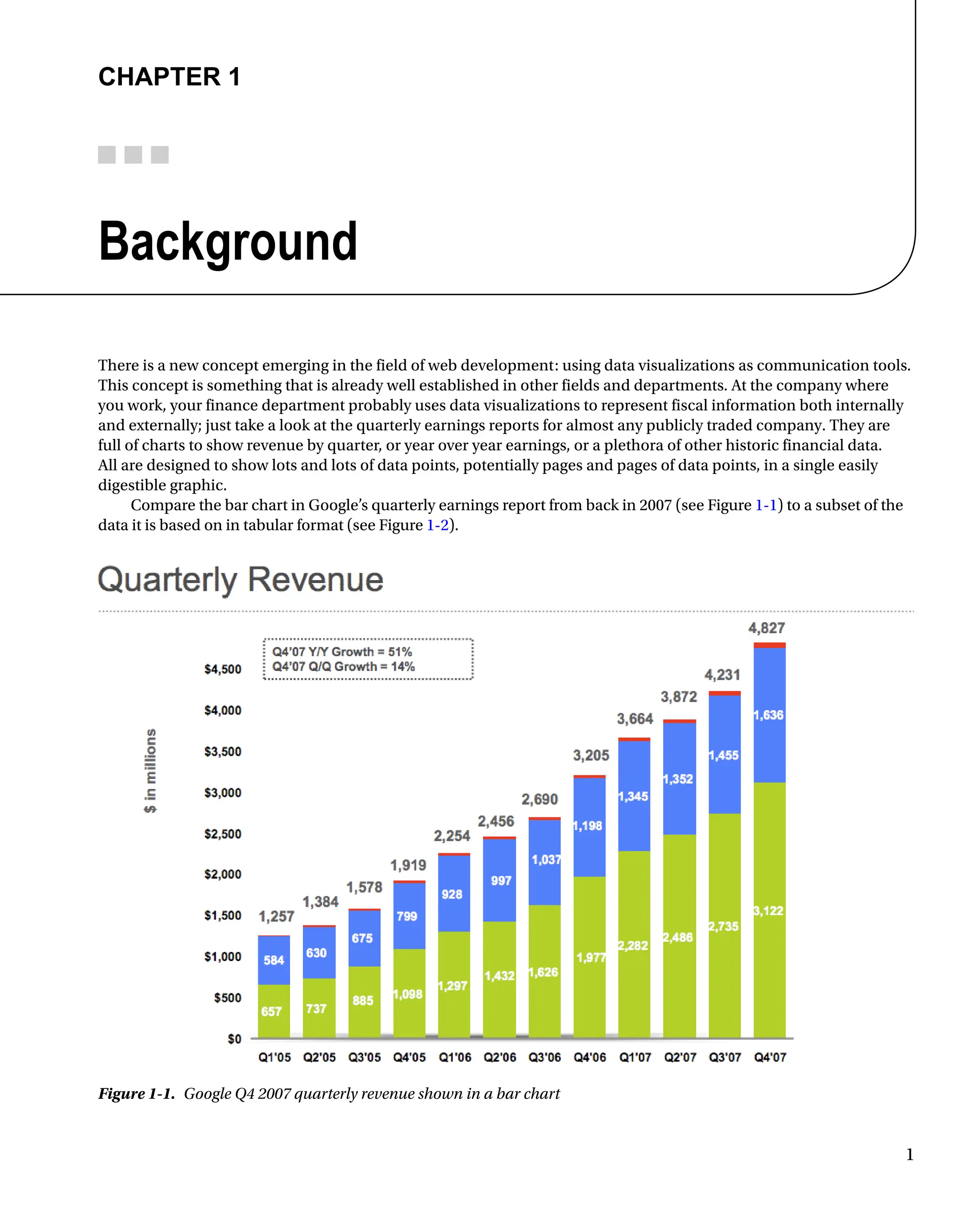
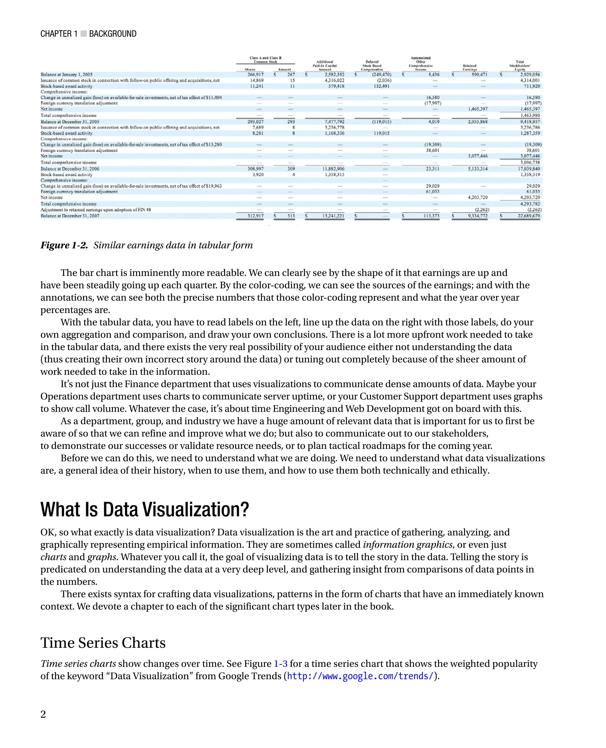
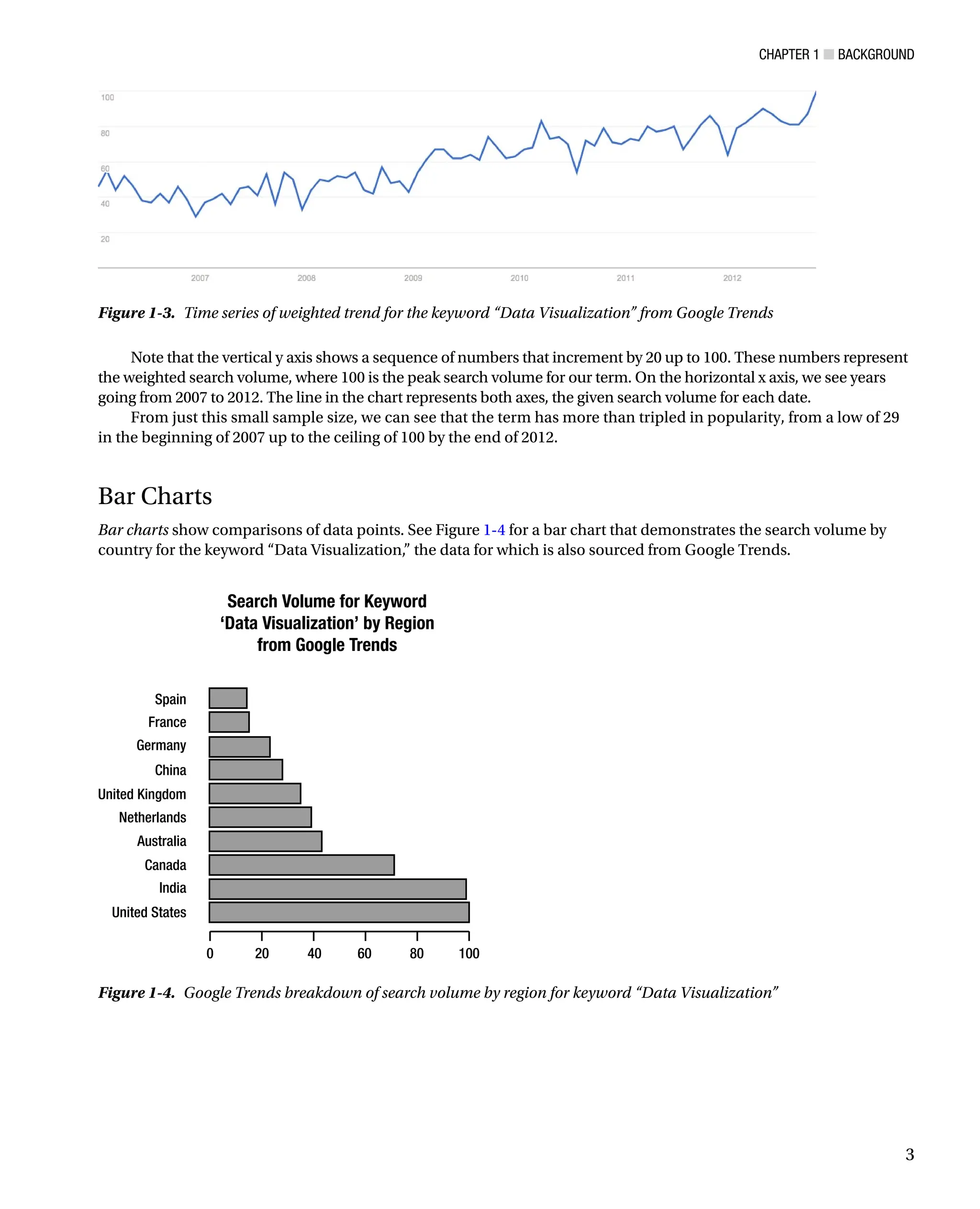
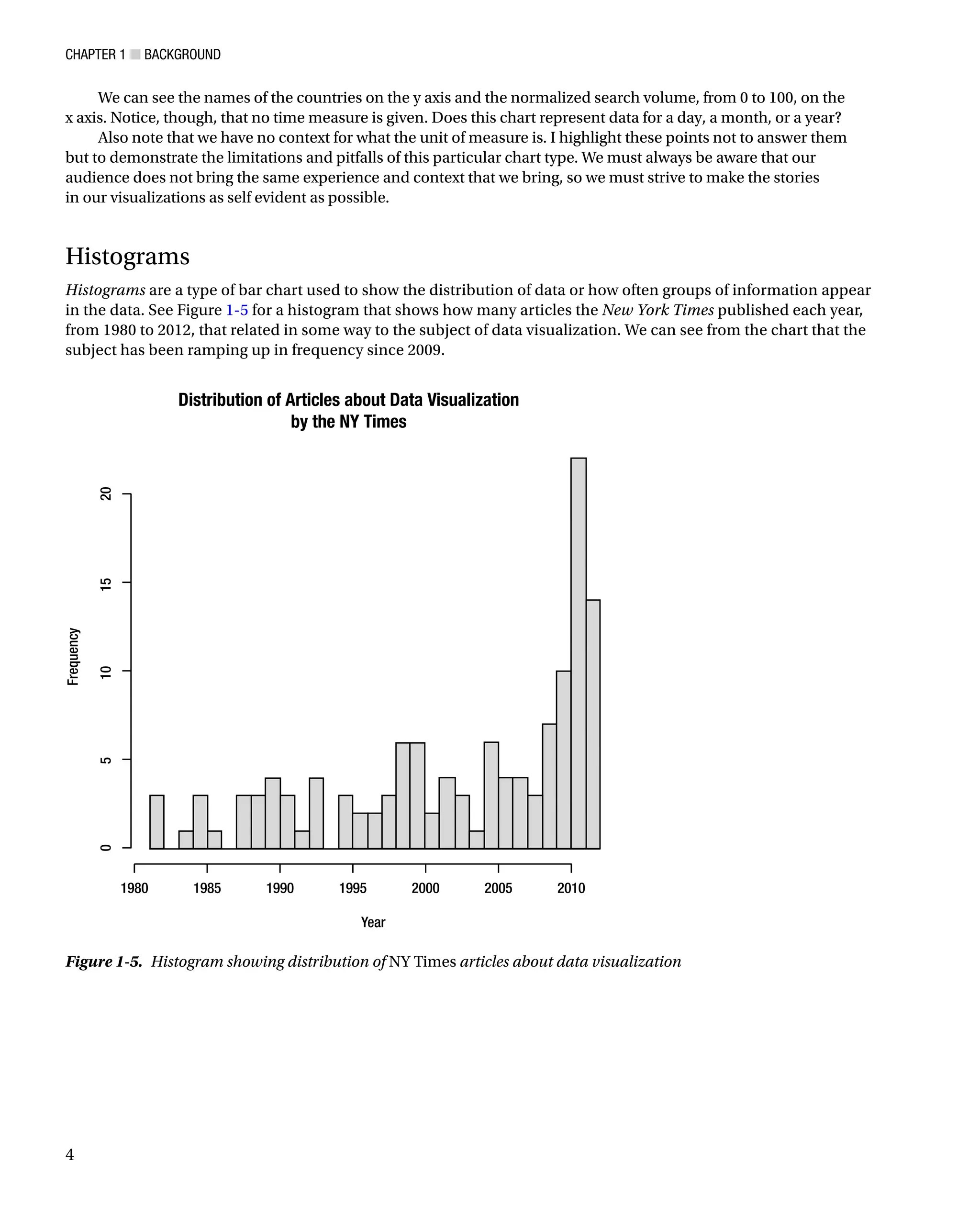
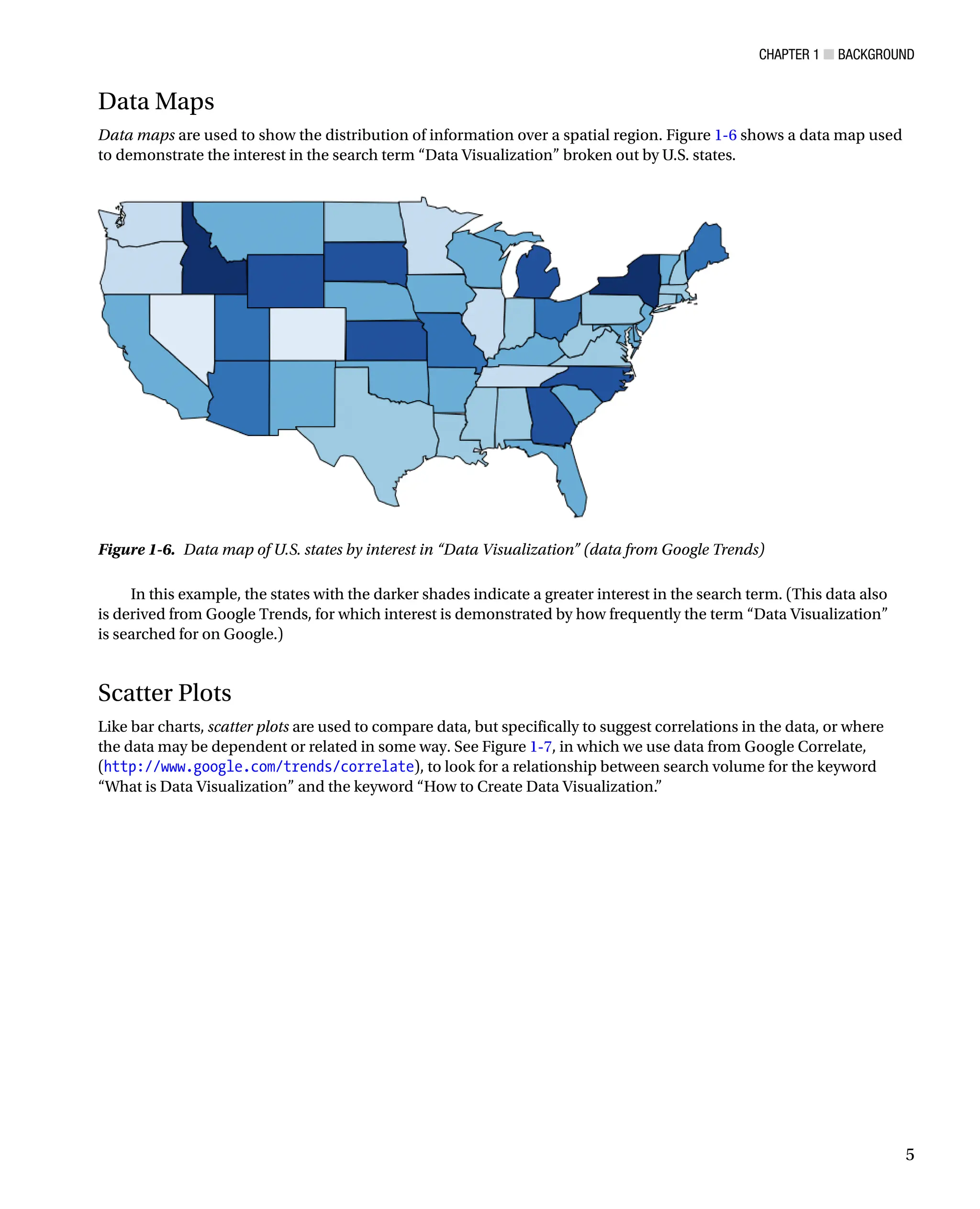
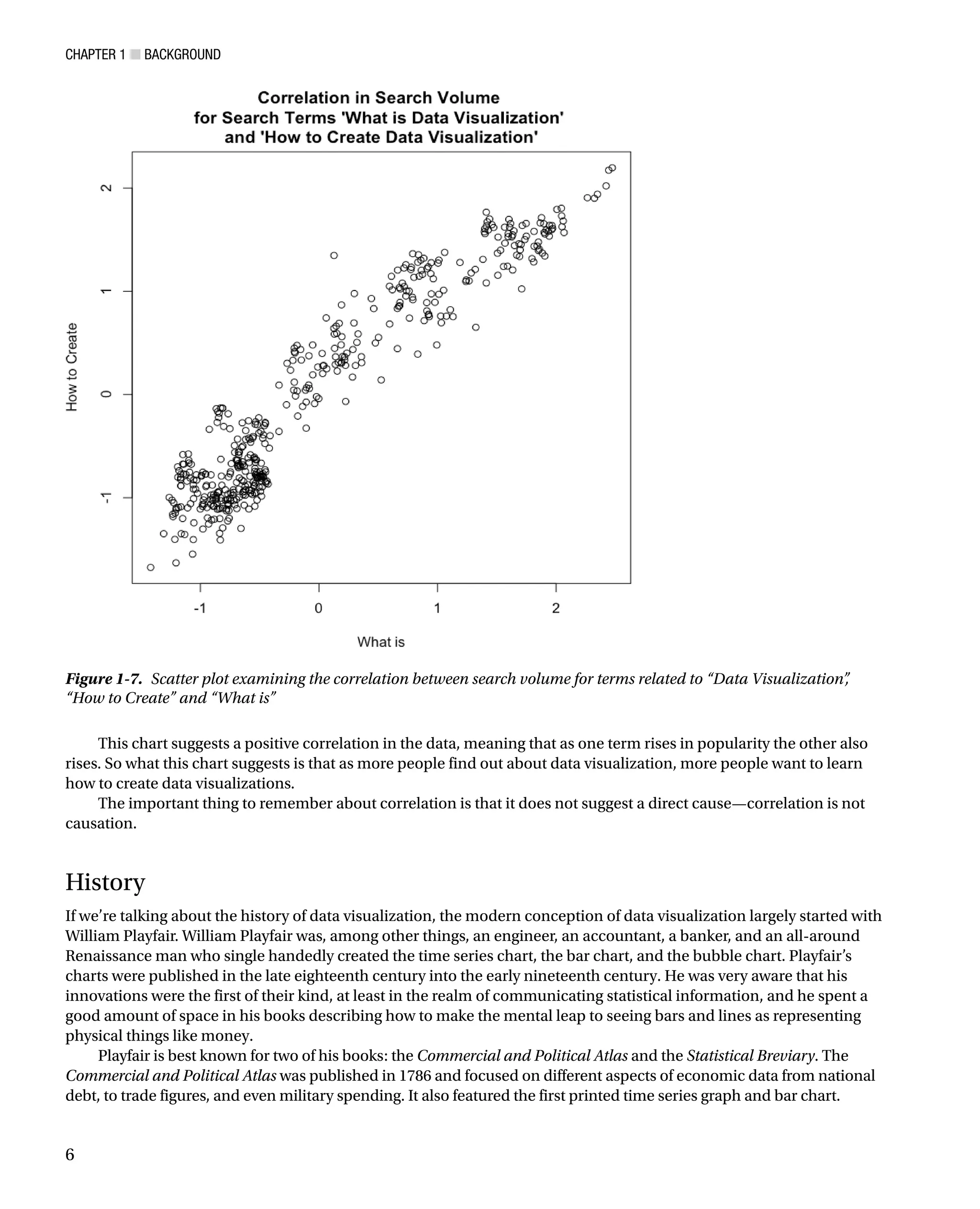

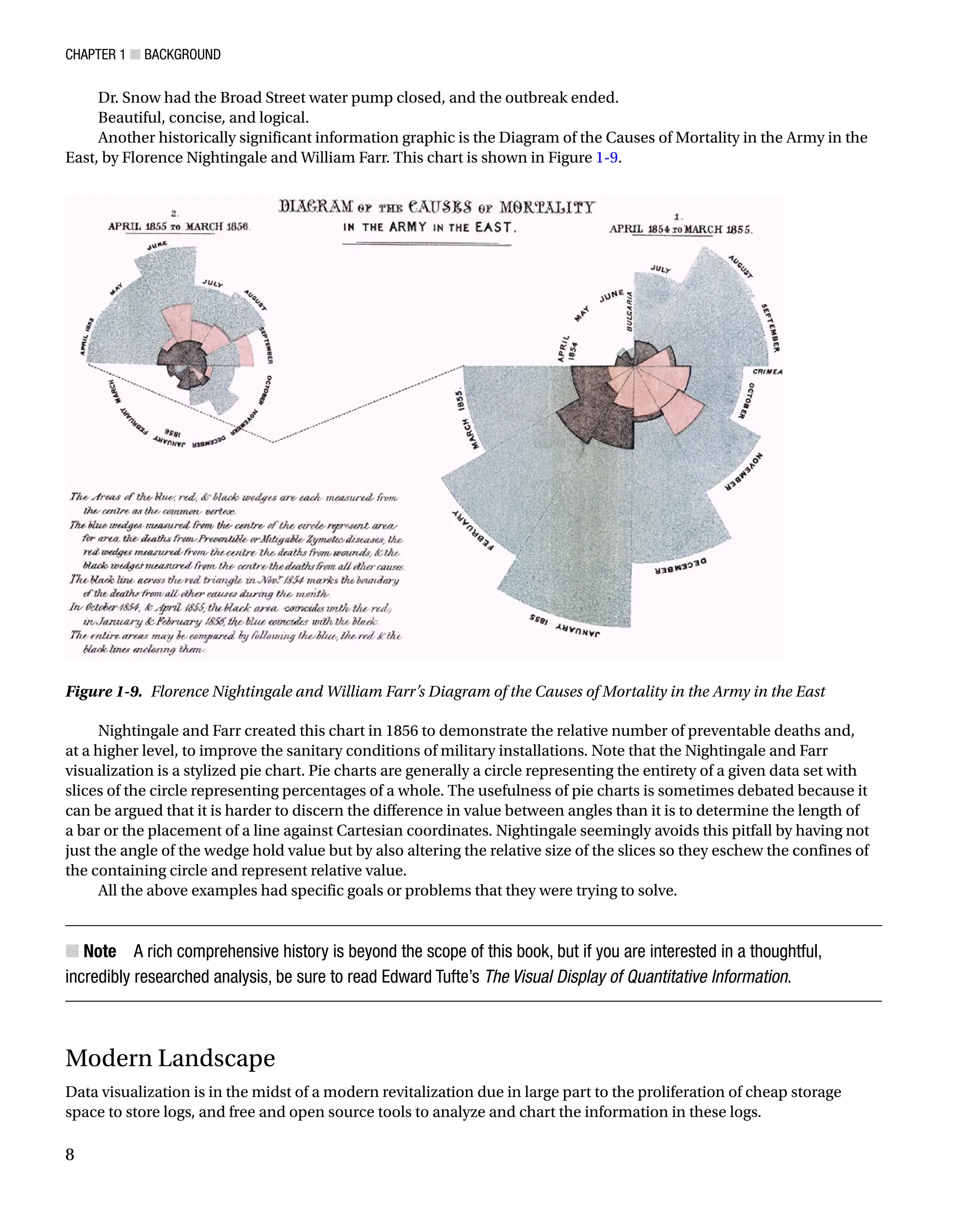
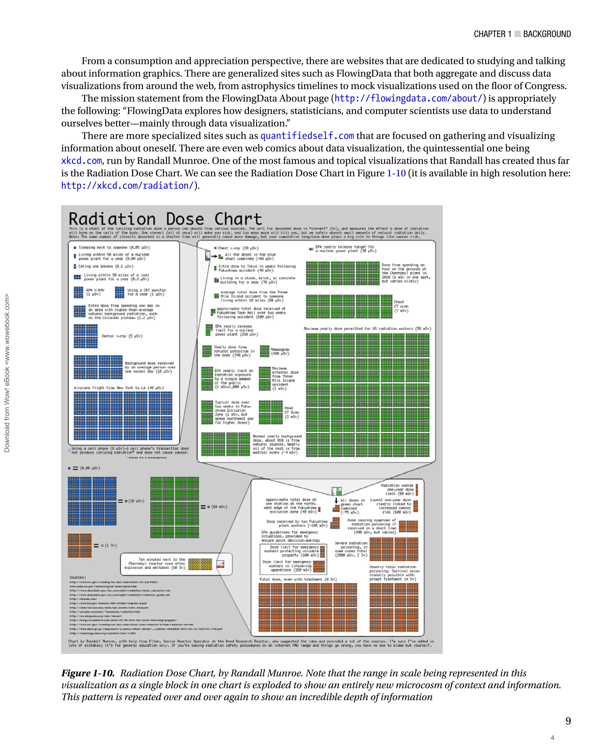
![Chapter 1 ■ Background
10
This chart was created in response to the Fukushima Daiichi nuclear disaster of 2011, and sought to clear up
misinformation and misunderstanding of comparisons being made around the disaster. It did this by demonstrating the
differences in scale for the amount of radiation from sources such as other people or a banana, up to what a fatal dose of
radiation ultimately would be—how all that compared to spending just ten minutes near the Chernobyl meltdown.
Over the last quarter of a century, Edward Tufte, author and professor emeritus at Yale University, has been
working to raise the bar of information graphics. He published groundbreaking books detailing the history of data
visualization, tracing its roots even further back than Playfair, to the beginnings of cartography. Among his principles
is the idea to maximize the amount of information included in each graphic—both by increasing the amount of
variables or data points in a chart and by eliminating the use of what he has coined chartjunk. Chartjunk, according to
Tufte, is anything included in a graph that is not information, including ornamentation or thick, gaudy arrows.
Tufte also invented the sparkline, a time series chart with all axes removed and only the trendline remaining to
show historic variations of a data point without concern for exact context. Sparklines are intended to be small enough
to place in line with a body of text, similar in size to the surrounding characters, and to show the recent or historic
trend of whatever the context of the text is.
Why Data Visualization?
In William Playfair’s introduction to the Commercial and Political Atlas, he rationalizes that just as algebra is the
abbreviated shorthand for arithmetic, so are charts a way to “abbreviate and facilitate the modes of conveying
information from one person to another.” Almost 300 years later, this principle remains the same.
Data visualizations are a universal way to present complex and varied amounts of information, as we saw in our
opening example with the quarterly earnings report. They are also powerful ways to tell a story with data.
Imagine you have your Apache logs in front of you, with thousands of lines all resembling the following:
127.0.0.1 - - [10/Dec/2012:10:39:11 +0300] GET / HTTP/1.1 200 468 - Mozilla/5.0 (X11; U;
Linux i686; en-US; rv:1.8.1.3) Gecko/20061201 Firefox/2.0.0.3 (Ubuntu-feisty)
127.0.0.1 - - [10/Dec/2012:10:39:11 +0300] GET /favicon.ico HTTP/1.1 200 766 - Mozilla/5.0
(X11; U; Linux i686; en-US; rv:1.8.1.3) Gecko/20061201 Firefox/2.0.0.3 (Ubuntu-feisty)
Among other things, we see IP address, date, requested resource, and client user agent. Now imagine this
repeated thousands of times—so many times that your eyes kind of glaze over because each line so closely resembles
the ones around it that it’s hard to discern where each line ends, let alone what cumulative trends exist within.
By using some analysis and visualization tools such as R, or even a commercial product such as Splunk, we can
artfully pull out all kinds of meaningful and interesting stories out of this log, from how often certain HTTP errors occur
and for which resources, to what our most widely used URLs are, to what the geographic distribution of our user base is.
This is just our Apache access log. Imagine casting a wider net, pulling in release information, bugs and
production incidents. What insights we could gather about what we do: from how our velocity impacts our defect
density to how our bugs are distributed across our feature sets. And what better way to communicate those findings
and tell those stories than through a universally digestible medium, like data visualizations?
The point of this book is to explore how we as developers can leverage this practice and medium as part of
continual improvement—both to identify and quantify our successes and opportunities for improvements, and more
effectively communicate our learning and our progress.
Tools
There are a number of excellent tools, environments, and libraries that we can use both to analyze and visualize our
data. The next two sections describe them.](https://image.slidesharecdn.com/5350-250413224758-767bf818/75/Pro-Data-Visualization-using-R-and-JavaScript-1st-Edition-Tom-Barker-17-2048.jpg)
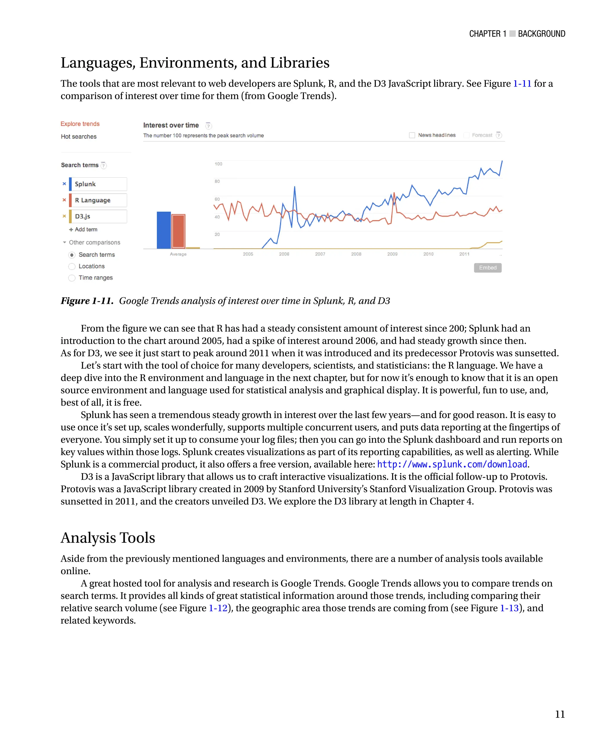
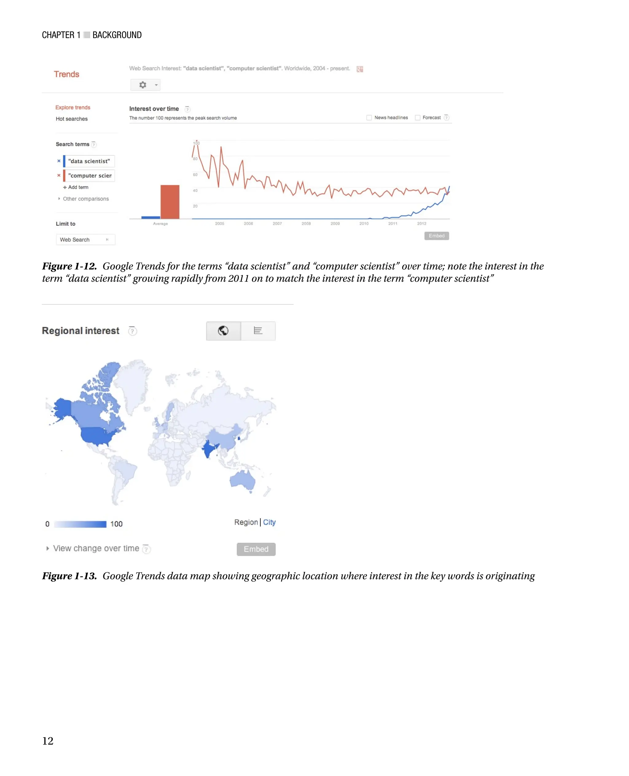

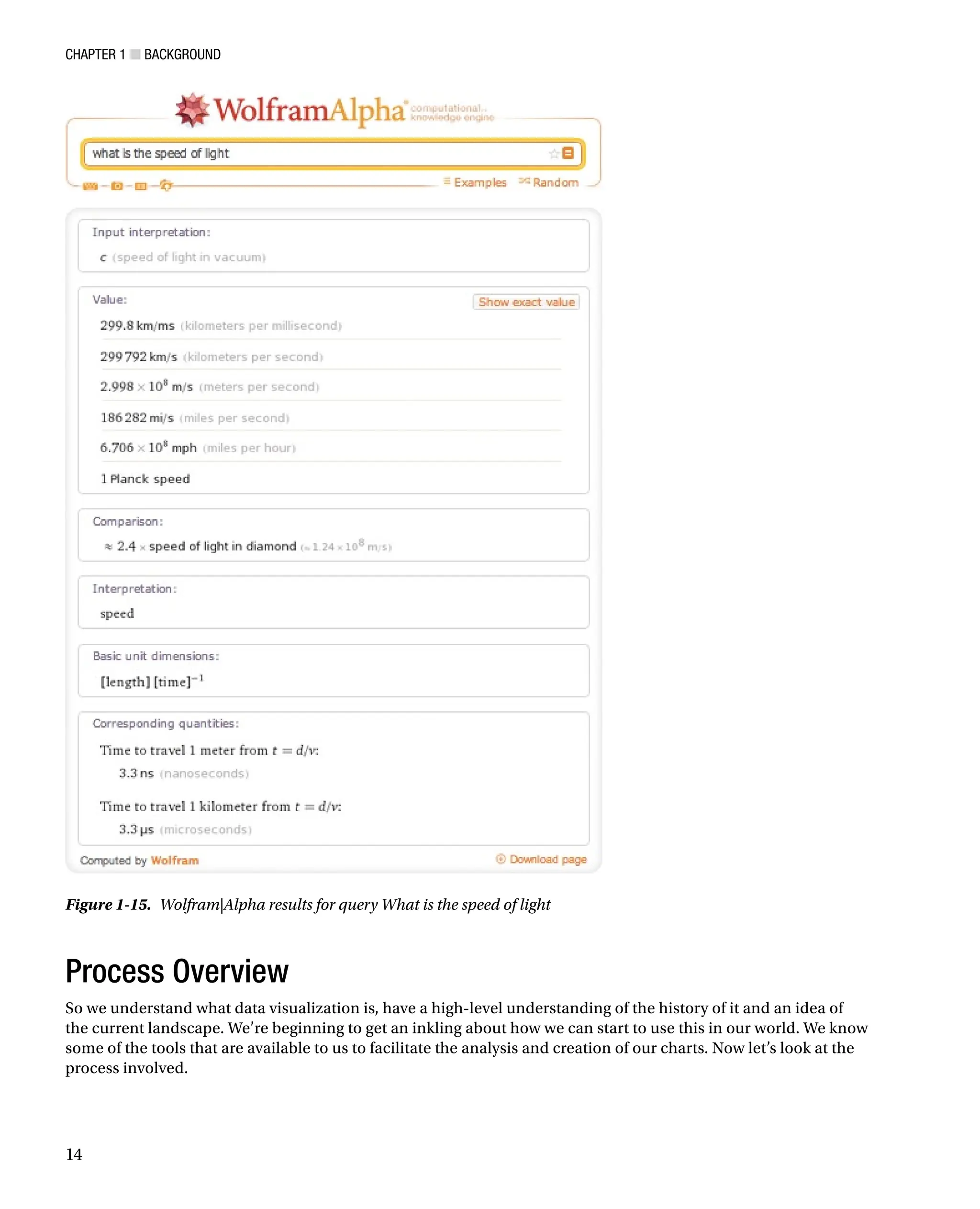
![Chapter 1 ■ Background
15
Creating data visualizations involves four core steps:
1. Identify a problem.
2. Gather the data.
3. Analyze the data.
4. Visualize the data.
Let’s walk through each step in the process and re-create one of the previous charts to demonstrate the process.
Identify a Problem
The very first step is to identify a problem we want to solve. This can be almost anything—from something as
profound and wide-reaching as figuring out why your bug backlog doesn’t seem to go down and stay down, to seeing
what feature releases over a given period in time caused the most production incidents, and why.
For our example, let’s re-create Figure 1-5 and try to quantify the interest in data visualization over time as
represented by the number of New York Times articles on the subject.
Gather Data
We have an idea of what we want to investigate, so let’s dig in. If you are trying to solve a problem or tell a story around
your own product, you would of course start with your own data—maybe your Apache logs, maybe your bug backlog,
maybe exports from your project tracking software.
Note
■
■ If you are focusing on gathering metrics around your product and you don’t already have data handy, you need to
invest in instrumentation.There are many ways to do this, usually by putting logging in your code.At the very least, you want to
log error states and monitor those, but you may want to expand the scope of what you track to include for
debugging purposes
while still respecting both your user’s privacy and your company’s privacy policy. In my book, Pro JavaScript
Performance:
Monitoring and Visualization, I explore ways to track and visualize web and runtime performance.
One important aspect of data gathering is deciding which format your data should be in (if you're lucky) or discovering
which format your data is available in. We’ll next be looking at some of the common data formats in use today.
JSON is an acronym that stands for JavaScript Object Notation. As you probably know, it is essentially a way to
send data as serialized JavaScript objects. We format JSON as follows:
[object]{
[attribute]: [value],
[method] : function(){},
[array]: [item, item]
}
Another way to transfer data is in XML format. XML has an expected syntax, in which elements can have attributes,
which have values, values are always in quotes, and every element must have a closing element. XML looks like this:
parent attribute=value
child attribute=valuenode data/child
/parent
Generally we can expect APIs to return XML or JSON to us, and our preference is usually JSON because as we can
see it is a much more lightweight option just in sheer amount of characters used.](https://image.slidesharecdn.com/5350-250413224758-767bf818/75/Pro-Data-Visualization-using-R-and-JavaScript-1st-Edition-Tom-Barker-22-2048.jpg)
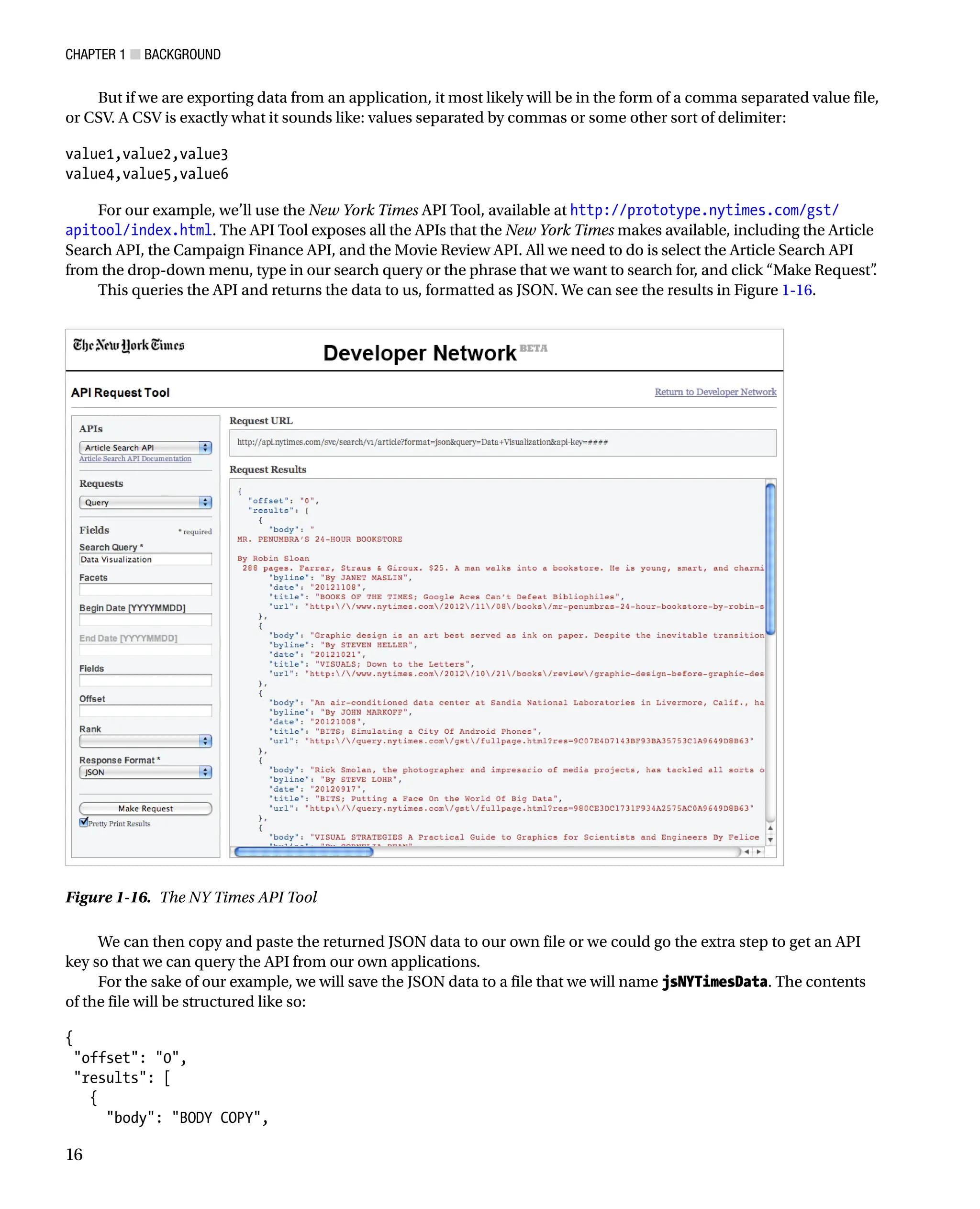
![Chapter 1 ■ Background
17
byline: By AUTHOR,
date: 20121011,
title: TITLE,
url: http://www.nytimes.com/foo.html
}, {
body: BODY COPY,
byline: By AUTHOR,
date: 20121021,
title: TITLE,
url: http://www.nytimes.com/bar.html
}
],
tokens: [
JavaScript
],
total: 2
}
Looking at the high-level JSON structure, we see an attribute named offset, an array named results, an array
named tokens, and another attribute named total. The offset variable is for pagination (what page full of results
we are starting with). The total variable is just what it sounds like: the number of results that are returned for our
query. It’s the results array that we really care about; it is an array of objects, each of which corresponds to an article.
The article objects have attributes named body, byline, date, title, and url.
We now have data that we can begin to look at. That takes us to our next step in the process, analyzing our data.
DATA SCRUBBING
There is often a hidden step here, one that anyone who’s dealt with data knows about: scrubbing the data. Often
the data is either not formatted exactly as we need it or, in even worse cases, it is dirty or incomplete.
In the best-case scenario in which your data just needs to be reformatted or even concatenated, go ahead and do
that, but be sure to not lose the integrity of the data.
Dirty data has fields out of order, fields with obviously bad information in them—think strings in ZIP codes—or
gaps in the data. If your data is dirty, you have several choices:
You could drop the rows in question, but that can harm the integrity of the data—a good example
•
is if you are creating a histogram removing rows could change the distribution and change what
your results will be.
The better alternative is to reach out to whoever administers the source of your data and try and
•
get a better version if it exists.
Whatever the case, if data is dirty or it just needs to be reformatted to be able to be imported into R, expect to
have to scrub your data at some point before you begin your analysis.
Analyze Data
Having data is great, but what does it mean? We determine it through analysis.
Analysis is the most crucial piece of creating data visualizations. It’s only through analysis that we can understand
our data, and it is only through understanding it that we can craft our story to share with others.](https://image.slidesharecdn.com/5350-250413224758-767bf818/75/Pro-Data-Visualization-using-R-and-JavaScript-1st-Edition-Tom-Barker-24-2048.jpg)
![Chapter 1 ■ BaCkground
19
if(length(author) 1){
author - unknown
}
datestamp -paste(month, /, day, /, year, sep=)
datestamp - as.Date(datestamp,%m/%d/%Y)
newrow - data.frame(datestamp, author, title, stringsAsFactors=FALSE, check.rows=FALSE)
df - rbind(df, newrow)
}
rownames(df) - df$datestamp
Note that our example assumes that the data set returned has unique date values. If you get errors with this, you
may need to scrub your returned data set to purge any duplicate rows.
Once our data frame is populated, we can start to do some analysis on the data. Let’s start out by pulling just the
year from every entry, and quickly making a stem and leaf plot to see the shape of the data.
Note John tukey created the stem and leaf plot in his seminal work, Exploratory Data Analysis. Stem and leaf plots
are quick, high-level ways to see the shape of data, much like a histogram. In the stem and leaf plot, we construct the
“stem” column on the left and the “leaf” column on the right. the stem consists of the most significant unique elements
in a result set. the leaf consists of the remainder of the values associated with each stem. In our stem and leaf plot below,
the years are our stem and r shows zeroes for each row associated with a given year. Something else to note is that
often alternating sequential rows are combined into a single row, in the interest of having a more concise visualization.
First, we will create a new variable to hold the year information:
yearlist - as.POSIXlt(df$datestamp)$year+1900
If we inspect this variable, we see that it looks something like this:
yearlist
[1] 2012 2012 2012 2012 2012 2012 2012 2012 2012 2012 2012 2012 2012 2011 2011 2011 2011 2011 2011
2011 2011 2011 2011 2011 2011 2011 2011 2011 2011
[30] 2011 2011 2011 2011 2010 2010 2010 2010 2010 2010 2010 2010 2010 2010 2009 2009 2009 2009 2009
2009 2009 2008 2008 2008 2007 2007 2007 2007 2006
[59] 2006 2006 2006 2005 2005 2005 2005 2005 2005 2004 2003 2003 2003 2002 2002 2002 2002 2001 2001
2000 2000 2000 2000 2000 2000 1999 1999 1999 1999
[88] 1999 1999 1998 1998 1998 1997 1997 1996 1996 1995 1995 1995 1993 1993 1993 1993 1992 1991 1991
1991 1990 1990 1990 1990 1989 1989 1989 1988 1988
[117] 1988 1986 1985 1985 1985 1984 1982 1982 1981
That’s great, that’s exactly what we want: a year to represent every article returned. Next let’s create the stem and
leaf plot:
stem(yearlist)
1980 | 0
1982 | 00
1984 | 0000
1986 | 0
1988 | 000000
Download
from
Wow!
eBook
www.wowebook.com](https://image.slidesharecdn.com/5350-250413224758-767bf818/75/Pro-Data-Visualization-using-R-and-JavaScript-1st-Edition-Tom-Barker-26-2048.jpg)
![Chapter 1 ■ Background
20
1990 | 0000000
1992 | 00000
1994 | 000
1996 | 0000
1998 | 000000000
2000 | 00000000
2002 | 0000000
2004 | 0000000
2006 | 00000000
2008 | 0000000000
2010 | 000000000000000000000000000000
2012 | 0000000000000
Very interesting. We see a gradual build with some dips in the mid-1990s, another gradual build with another dip
in the mid-2000s and a strong explosion since 2010 (the stem and leaf plot groups years together in twos).
Looking at that, my mind starts to envision a story building about a subject growing in popularity. But what
about the authors of these articles? Maybe they are the result of one or two very interested authors that have quite
a bit to say on the subject.
Let’s explore that idea and take a look at the author data that we parsed out. Let’s look at just the unique authors
from our data frame:
length(unique(df$author))
[1] 81
We see that there are 81 unique authors or combination of authors for these articles! Just out of curiosity, let’s take
a look at the breakdown by author for each article. Let’s quickly create a bar chart to see the overall shape of the data
(the bar chart is shown in Figure 1-17):
plot(table(df$author), axes=FALSE)
Figure 1-17. Bar chart of number of articles by author to quickly visualize](https://image.slidesharecdn.com/5350-250413224758-767bf818/75/Pro-Data-Visualization-using-R-and-JavaScript-1st-Edition-Tom-Barker-27-2048.jpg)
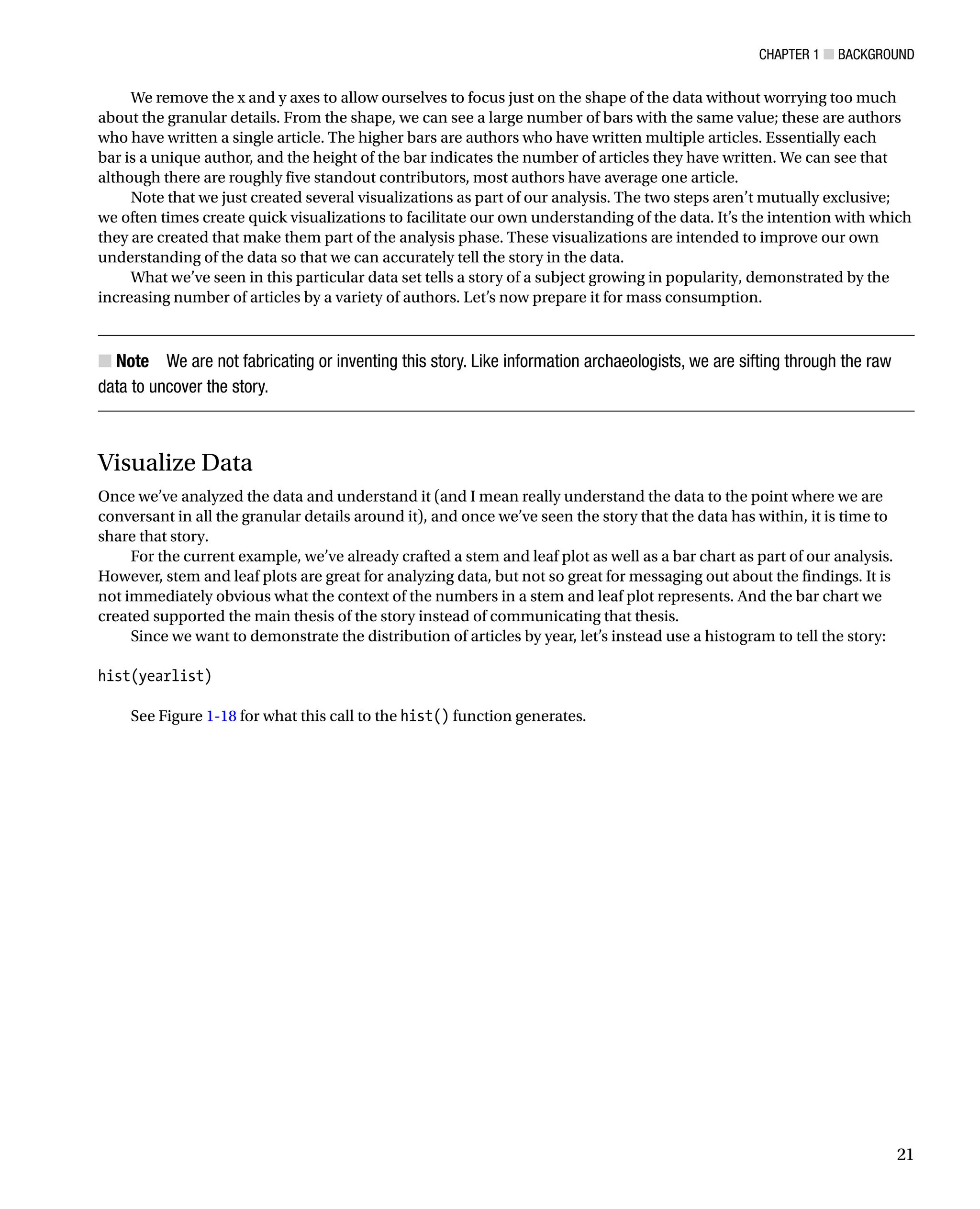
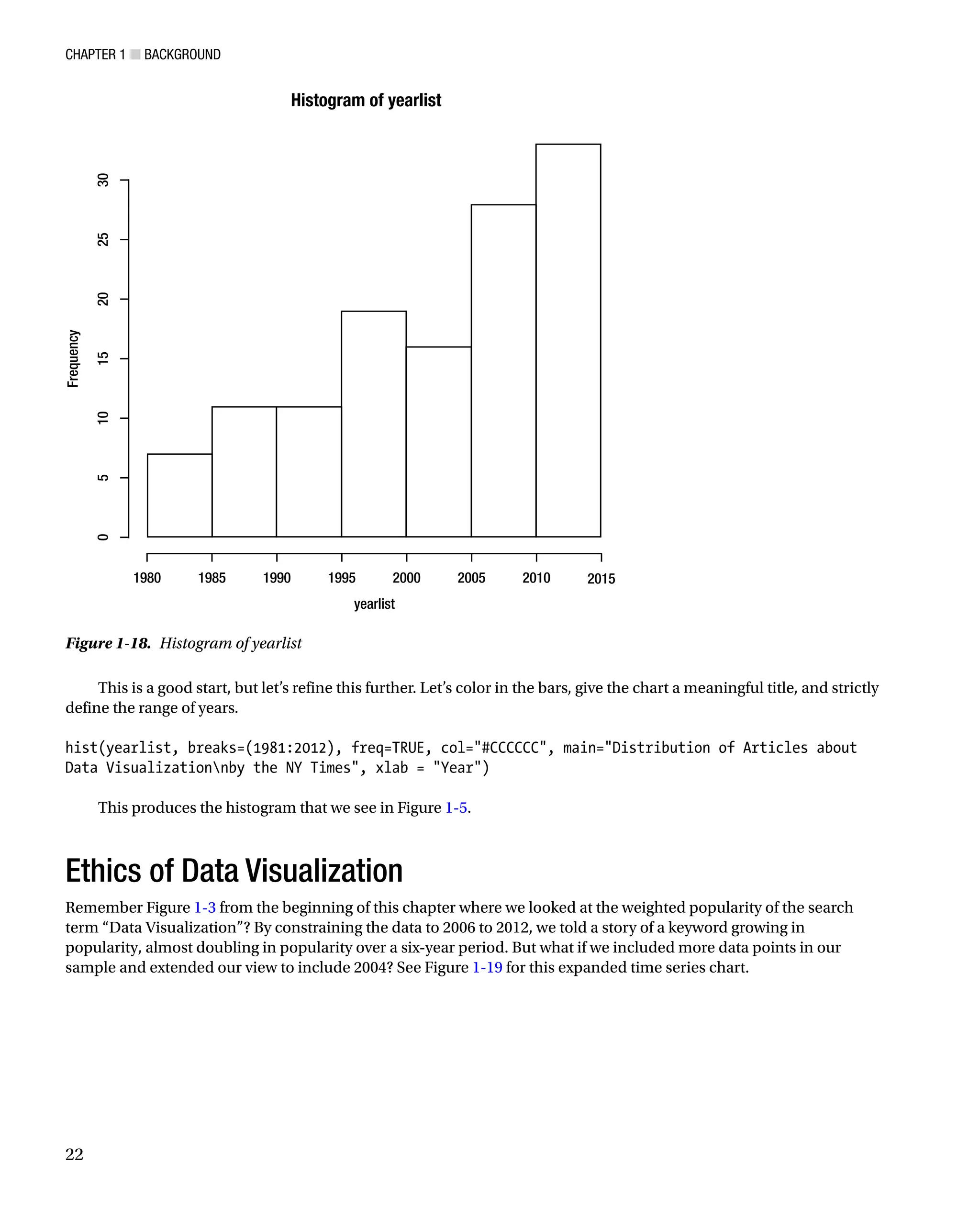
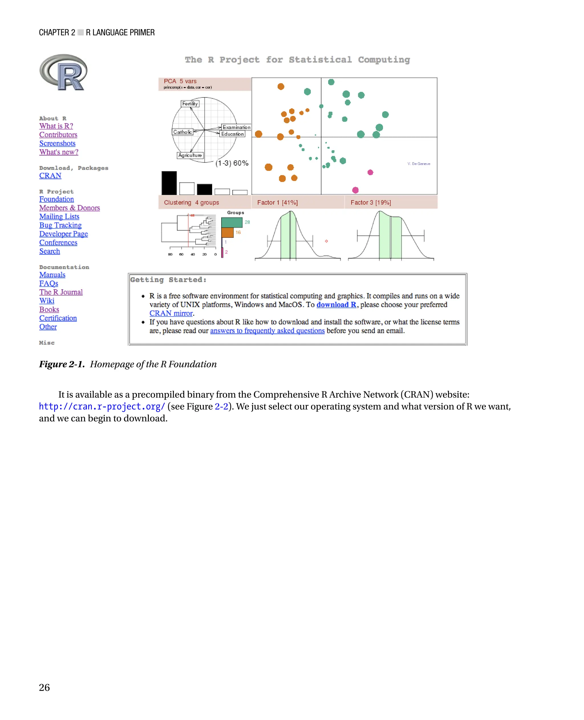

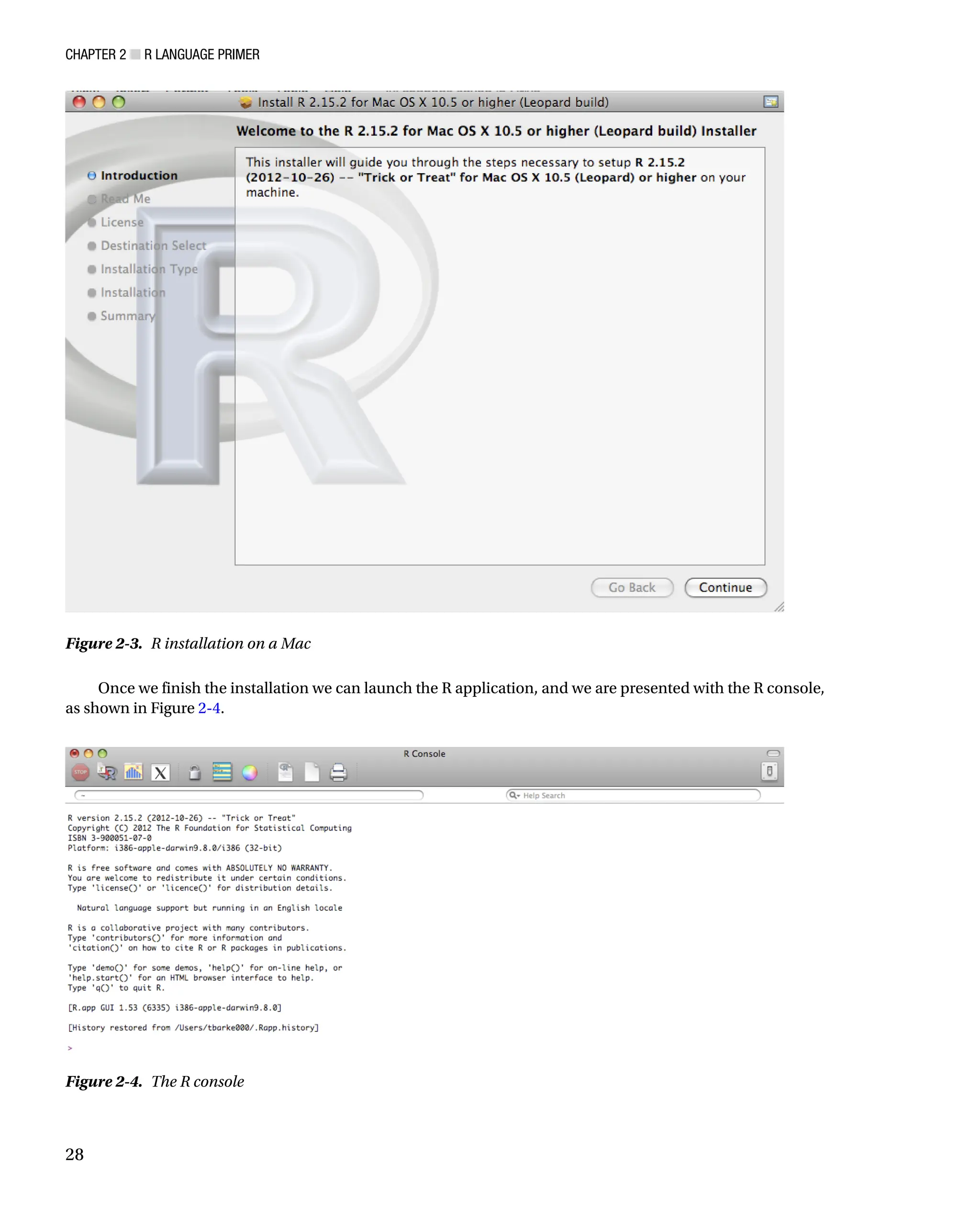
![Chapter 2 ■ R Language Primer
29
The Command Line
The R console is where the magic happens! It is a command-line environment where we can run R expressions. The best
way to get up to speed in R is to script in the console, a piece at a time, generally to try out what you’re trying to do, and
tweak it until you get the results that you want. When you finally have a working example, take the code that does what
you want and save it as an R script file.
R script files are just files that contain pure R and can be run in the console using the source command:
source(someRfile.R)
Looking at the preceding code snippet, we assume that the R script lives in the current work directory. The way
we can see what the current work directory is to use the getwd() function:
getwd()
[1] /Users/tomjbarker
We can also set the working directory by using the setwd() function. Note that changes made to the working
directory are not persisted across R sessions unless the session is saved.
setwd(/Users/tomjbarker/Downloads)
getwd()
[1] /Users/tomjbarker/Downloads
Command History
The R console stores commands that you enter and you can cycle through previous commands by pressing the up
arrow. Hit the escape button to return to the command prompt. We can see the history in a separate window pane
by clicking the Show/Hide Command History button at the top of the console. The Show/Hide Command History
button is the rectangle icon with alternating stripes of yellow and green. See Figure 2-5 for the R console with the
command history shown.](https://image.slidesharecdn.com/5350-250413224758-767bf818/75/Pro-Data-Visualization-using-R-and-JavaScript-1st-Edition-Tom-Barker-35-2048.jpg)
![Chapter 2 ■ R Language Primer
31
Packages
Speaking of packages, what are they, exactly? Packages are collections of functions, data sets, or objects that can
be imported into the current session or workspace to extend what we can do in R. Anyone can make a package
and distribute it.
To install a package, we simply type this:
install.packages([package name])
For example, if we want to install the ggplot2 package—which is a widely used and very handy charting
package—we simply type this into the console:
install.packages(ggplot2)
We are immediately prompted to choose the mirror location that we want to use, usually the one closest to our
current location. From there, the install begins. We can see the results in Figure 2-7.
Figure 2-6. Help search results window](https://image.slidesharecdn.com/5350-250413224758-767bf818/75/Pro-Data-Visualization-using-R-and-JavaScript-1st-Edition-Tom-Barker-37-2048.jpg)
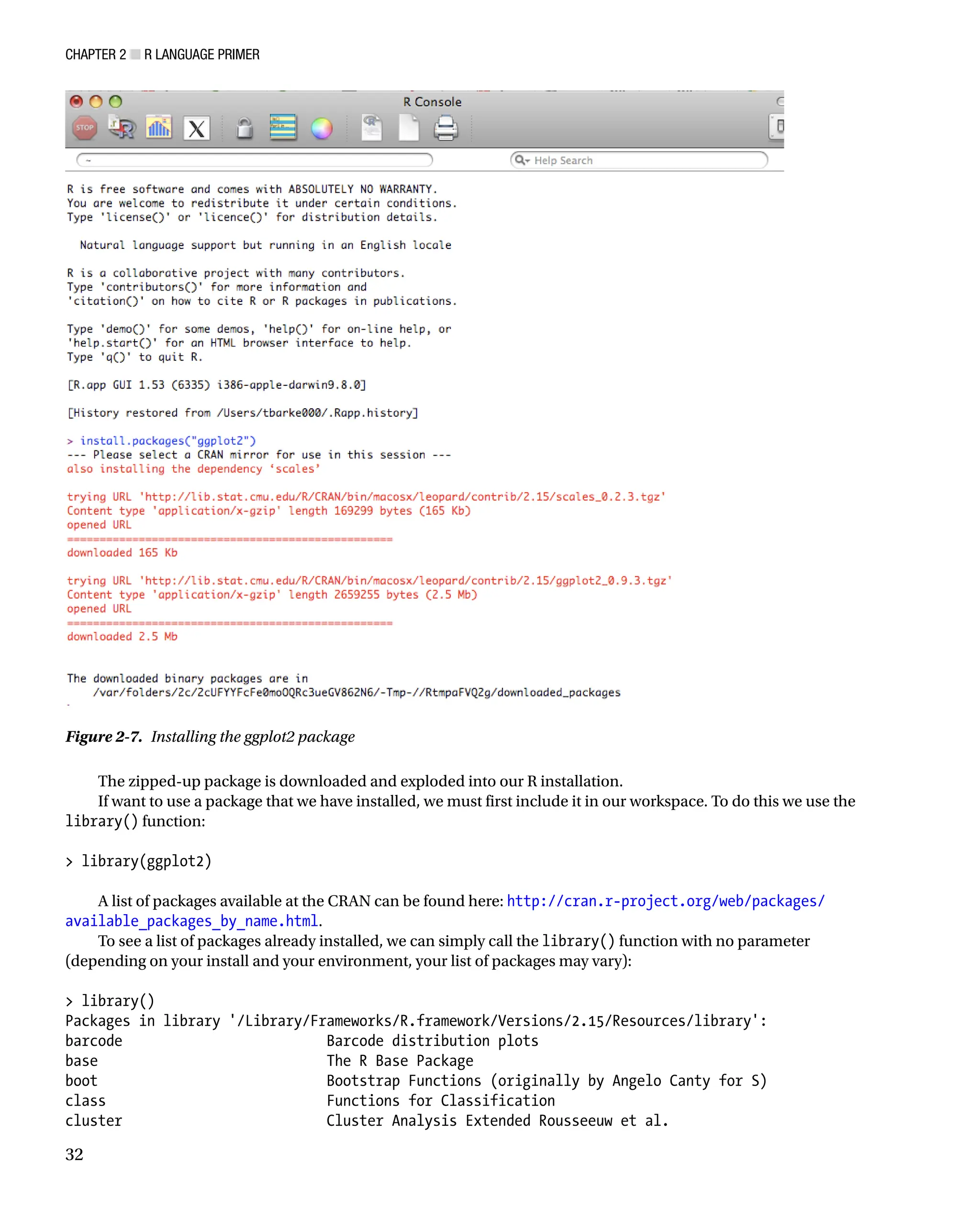
![Chapter 2 ■ R Language Primer
33
codetools Code Analysis Tools for R
colorspace Color Space Manipulation
compiler The R Compiler Package
datasets The R Datasets Package
dichromat Color schemes for dichromats
digest Create cryptographic hash digests of R objects
foreign Read Data Stored by Minitab, S, SAS, SPSS, Stata, Systat, dBase,
...
ggplot2 An implementation of the Grammar of Graphics
gpairs gpairs: The Generalized Pairs Plot
graphics The R Graphics Package
grDevices The R Graphics Devices and Support for Colours and Fonts
grid The Grid Graphics Package
gtable Arrange grobs in tables.
KernSmooth Functions for kernel smoothing for Wand Jones (1995)
labeling Axis Labeling
lattice Lattice Graphics
mapdata Extra Map Databases
mapproj Map Projections
maps Draw Geographical Maps
Importing Data
So now our environment is downloaded and installed, and we know how to install any packages that we may need.
Now we can begin using R.
The first thing we’ll normally want to do is import your data. There are several ways to import data, but the most
common way is to use the read() function, which has several flavors:
read.table([file to read])
read.csv([file to read])
To see this in action, let’s first create a text file named temptext.txt that is formatted like so:
134,432,435,313,11
403,200,500,404,33
77,321,90,2002,395
We can read this into a variable that we will name temptxt:
temptxt - read.table(temptext.txt)
Notice that as we are assigning value to this variable, we are not using an equal sign as the assignment operator.
We are instead using an arrow -. That is R’s assignment operator, although it does also support the equal sign if you
are so inclined. But the standard is the arrow, and all examples that we will show in this book will use the arrow.
If we print out the temptxt variable, we see that it is structured as follows:
temptxt
V1
1 134,432,435,313,11
2 403,200,500,404,33
3 77,321,90,2002,395](https://image.slidesharecdn.com/5350-250413224758-767bf818/75/Pro-Data-Visualization-using-R-and-JavaScript-1st-Edition-Tom-Barker-39-2048.jpg)
![Chapter 2 ■ R Language Primer
34
We see that our variable is a table-like structure called a data frame, and R has assigned a column name (V1) and
row IDs to our data structure. More on column names soon.
The read() function has a number of parameters that you can use to refine how the data is imported and
formatted once it is imported.
Using Headers
The header parameter tells R to treat the first line in the external file as containing header information. The first line
then becomes the column names of the data frame.
For example, suppose we have a log file structured like this:
url, day, date, loadtime, bytes, httprequests, loadtime_repeatview
http://apress.com, Sun, 01 Jul 2012 14:01:28 +0000,7042,956680,73,3341
http://apress.com, Sun, 01 Jul 2012 14:01:31 +0000,6932,892902,76,3428
http://apress.com, Sun, 01 Jul 2012 14:01:33 +0000,4157,594908,38,1614
We can load it into a variable named wpo like so:
wpo - read.table(wpo.txt, header=TRUE)
wpo
url day date loadtime bytes httprequests loadtime_repeatview
1 http://apress.com,Sun,1 Jul 2012 14:01:28 +0000,7042,955550,73,3191
2 http://apress.com,Sun,1 Jul 2012 14:01:31 +0000,6932,892442,76,3728
3 http://apress.com,Sun,1 Jul 2012 14:01:33 +0000,4157,614908,38,1514
When we call the colnames() function to see what the column names are for wpo, we see the following:
colnames(wpo)
[1] url day date loadtime
[5] bytes httprequests loadtime_repeatview
Specifying a String Delimiter
The sep attribute tells the read() function what to use as the string delimiter for parsing the columns in the external
data file. In all the examples we’ve looked at so far, commas are our delimiters, but we could use instead pipes | or any
other character that we want.
Say, for example, that our previous temptxt example used pipes; we would just update the code to be as follows:
134|432|435|313|11
403|200|500|404|33
77|321|90|2002|395
temptxt - read.table(temptext.txt, sep=|)
temptxt
V1 V2 V3 V4 V5
1 134 432 435 313 11
2 403 200 500 404 33
3 77 321 90 2002 395
Oh, notice that? We actually got distinct column names this time (V1, V2, V3, V4, V5). Before, we didn’t specify a
delimiter, so R assumed that each row was one big blob of text and lumped it into a single column (V1).](https://image.slidesharecdn.com/5350-250413224758-767bf818/75/Pro-Data-Visualization-using-R-and-JavaScript-1st-Edition-Tom-Barker-40-2048.jpg)
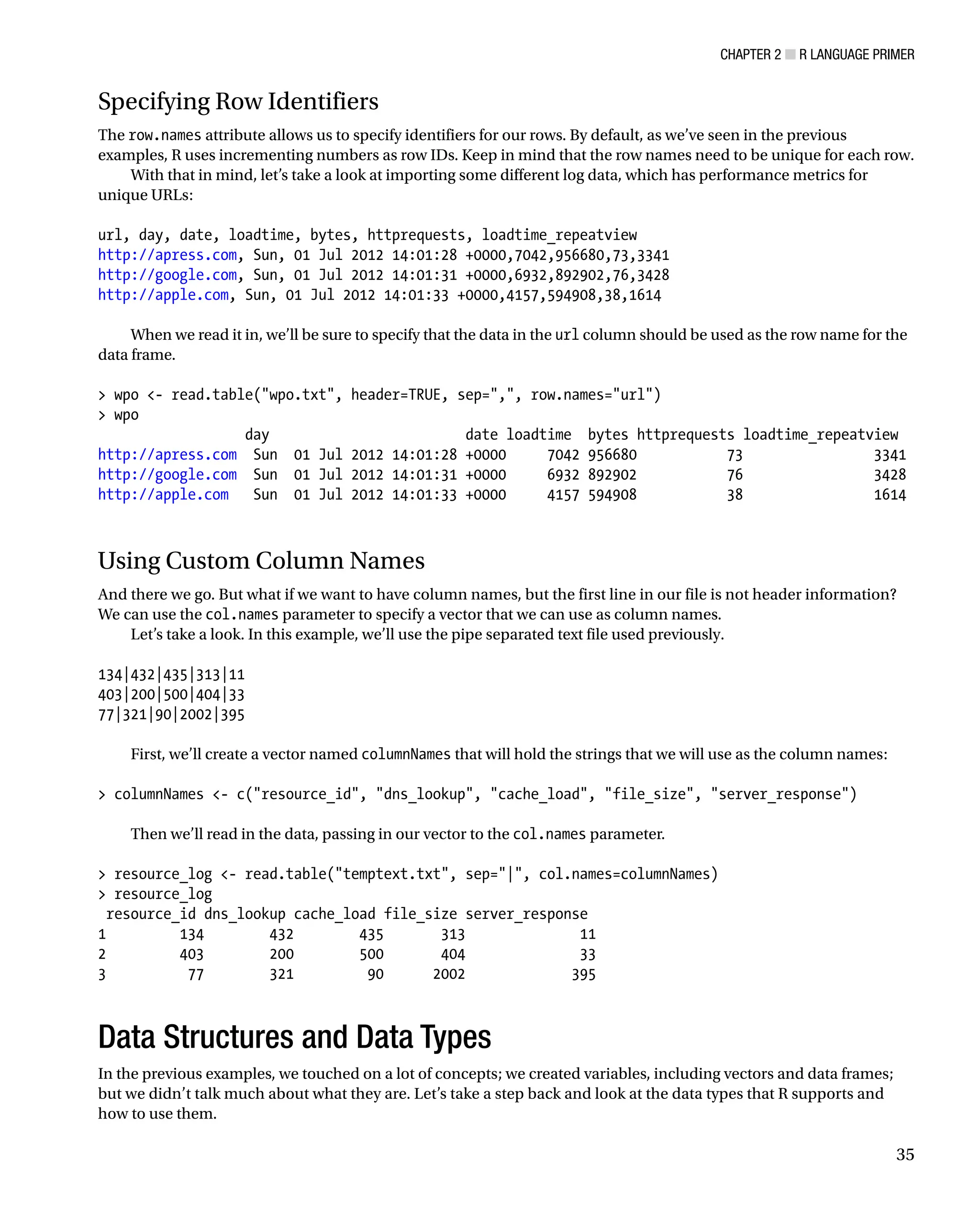
![Chapter 2 ■ R Language Primer
36
Data types in R are called modes, and can be the following:
numeric
•
character
•
logical
•
complex
•
raw
•
list
•
We can use the mode() function to check the mode of a variable.
Character and numeric modes correspond to string and number (both integer and float) data types. Logical
modes are Boolean values.
n - 122132
mode(n)
[1] numeric
c - test text
mode(c)
[1] character
l - TRUE
mode(l)
[1] logical
We can perform string concatenation using the paste() function. We can use the substr() function to pull
characters out of strings. Let’s look at some examples in code.
Usually, I keep a list of directories that I either read data from or write charts to. Then when I want to reference
a new data file that exists in the data directory, I will just append the new file name to the data directory:
dataDirectory - /Users/tomjbarker/org/data/
buglist - paste(dataDirectory, bugs.txt, sep=)
buglist
[1] /Users/tomjbarker/org/data/bugs.txt
The paste() function takes N amount of strings and concatenates them together. It accepts an argument named
sep that allows us to specify a string that we can use to be a delimiter between joined strings. We don’t want anything
separating our joined strings that we pass in an empty string.
If we want to pull characters from a string, we use the substr() function. The substr() function takes a string to
parse, a starting location, and a stopping location. It returns all the character inclusively from the starting location up
to the ending location. (Remember that in R, lists are not 0-based like most other languages, but instead have
a starting index of 1.)
substr(test, 1,2)
[1] te
In the preceding example, we pass in the string “test” and tell the substr() function to return the first and
second characters.
Complex mode is for complex numbers. The raw mode is to store raw byte data.](https://image.slidesharecdn.com/5350-250413224758-767bf818/75/Pro-Data-Visualization-using-R-and-JavaScript-1st-Edition-Tom-Barker-42-2048.jpg)
![Chapter 2 ■ R Language Primer
37
List data types or modes can be one of three classes: vectors, matrices, or data frames. If we call mode() for vectors
or matrices, they return the mode of the data that they contain; class() returns the class. If we call mode() on a data
frame, it returns the type list:
v - c(1:10)
mode(v)
[1] numeric
m - matrix(c(1:10), byrow=TRUE)
mode(m)
[1] numeric
class(m)
[1] matrix
d - data.frame(c(1:10))
mode(d)
[1] list
class(d)
[1] data.frame
Note that we just typed 1:10 rather than the whole sequence of numbers between 1 and 10:
v - c(1:10)
Vectors are single-dimensional arrays that can hold only values of a single mode at a time. It’s when we get to
data frames and matrices that R really starts to get interesting. The next two sections cover those classes.
Data Frames
We saw at the beginning of this chapter that the read() function takes in external data and saves it as a data frame.
Data frames are like arrays in most other loosely typed languages: they are containers that hold different types of data,
referenced by index. The main thing to realize, though, is that data frames see the data that they contain as rows, columns,
and combinations of the two.
For example, think of a data frame as formatted as follows:
col col col col col
row [ 1 ] [ 1 ] [ 1 ] [ 1 ] [ 1 ]
row [ 1 ] [ 1 ] [ 1 ] [ 1 ] [ 1 ]
row [ 1 ] [ 1 ] [ 1 ] [ 1 ] [ 1 ]
row [ 1 ] [ 1 ] [ 1 ] [ 1 ] [ 1 ]
If we try to reference the first index in the preceding data frame as we traditionally would with an array, say
dataframe[1], R would instead return the first column of data, not the first item. So data frames are referenced by their
column and row. So dataframe[1] returns the first column and dataframe[,2] returns the first row.
Let’s demonstrate this in code.
First let’s create some vectors using the combine function, c(). Remember that vectors are collections of data all
of the same type. The combine function takes a series of values and combines them into vectors.
col1 - c(1,2,3,4,5,6,7,8)
col2 - c(1,2,3,4,5,6,7,8)
col3 - c(1,2,3,4,5,6,7,8)
col4 - c(1,2,3,4,5,6,7,8)](https://image.slidesharecdn.com/5350-250413224758-767bf818/75/Pro-Data-Visualization-using-R-and-JavaScript-1st-Edition-Tom-Barker-43-2048.jpg)
![Chapter 2 ■ R Language Primer
38
Then let’s combine these vectors into a data frame:
df - data.frame(col1,col2,col3,col4)
Now let’s print the data frame to see the contents and the structure of it:
df
col1 col2 col3 col4
1 1 1 1 1
2 2 2 2 2
3 3 3 3 3
4 4 4 4 4
5 5 5 5 5
6 6 6 6 6
7 7 7 7 7
8 8 8 8 8
Notice that it took each vector and made each one a column. Also notice that each row has an ID; by default,
it is a number, but we can override that.
If we reference the first index, we see that the data frame returns the first column:
df[1]
col1
1 1
2 2
3 3
4 4
5 5
6 6
7 7
8 8
If we put a comma in front of that 1, we reference the first row:
df[,1]
[1] 1 2 3 4 5 6 7 8
So accessing contents of a data frame is done by specifying [column, row].
Matrices work much the same way.
Matrices
Matrices are just like data frames in that they contain rows and columns and can be referenced by either. The core
difference between the two is that data frames can hold different data types but matrices can hold only one type of data.
This presents a philosophical difference. Usually you use data frames to hold data read in externally, like from a
flat file or a database because those are generally of mixed type. You normally store data in matrices that you want to
apply functions to (more on applying functions to lists in a little bit).](https://image.slidesharecdn.com/5350-250413224758-767bf818/75/Pro-Data-Visualization-using-R-and-JavaScript-1st-Edition-Tom-Barker-44-2048.jpg)
![Chapter 2 ■ R Language Primer
39
To create a matrix, we must use the matrix() function, pass in a vector, and tell the function how to distribute
the vector:
The
• nrow parameter specifies how many rows the matrix should have
The
• ncol parameter specifies the number of columns.
The
• byrow parameter tells R that the contents of the vector should be distributed by iterating
across rows if TRUE or by columns if FALSE.
content - c(1,2,3,4,5,6,7,8,9,10)
m1 - matrix(content, nrow=2, ncol=5, byrow=TRUE)
m1
[,1] [,2] [,3] [,4] [,5]
[1,] 1 2 3 4 5
[2,] 6 7 8 9 10
Notice that in the previous example that the m1 matrix is filled in horizontally, row by row. In the following
example, the m1 matrix is filled in vertically by column:
content - c(1,2,3,4,5,6,7,8,9,10)
m1 - matrix(content, nrow=2, ncol=5, byrow=FALSE)
m1
[,1] [,2] [,3] [,4] [,5]
[1,] 1 3 5 7 9
[2,] 2 4 6 8 10
Remember that instead of manually typing out all the numbers in the previous content vector, if the numbers are
a sequence we can just type this:
content - (1:10)
We reference the content in matrices with the square bracket, specifying the row and column, respectively.
m1[1,4]
[1] 7
We can convert a data frame to a matrix if the data frame contains only a single type of data. To do this we use the
as.matrix() function. Often times we will do this when passing a data frame to a plotting function to draw a chart.
barplot(as.matrix(df))
Below we create a data frame called df. We populate the data frame with ten consecutive numbers. We then use
as.matrix() to convert df into a matrix and save the result into a new variable called m:
df - data.frame(1:10)
df
X1.10
1 1
2 2
3 3](https://image.slidesharecdn.com/5350-250413224758-767bf818/75/Pro-Data-Visualization-using-R-and-JavaScript-1st-Edition-Tom-Barker-45-2048.jpg)
![Chapter 2 ■ r Language primer
40
4 4
5 5
6 6
7 7
8 8
9 9
10 10
class(df)
[1] data.frame
m - as.matrix(df)
class(m)
[1] matrix
Keep in mind that because they are all the same data type, matrices require less overhead and are intrinsically
more efficient than data frames. If we compare the size of our matrix m and our data frame df, we see that with just ten
items there is a size difference.
object.size(m)
312 bytes
object.size(df)
440 bytes
With that said, if we increase the scale of this, the increase in efficiency does not equally scale. Compare the following:
big_df - data.frame(1:40000000)
big_m - matrix(1:40000000)
object.size(big_m)
160000112 bytes
object.size(big_df)
160000400 bytes
We can see that the first example with the small data set showed that the matrix was 30 percent smaller in size
than the data frame, but at the larger scale in the second example the matrix was only .00018 percent smaller than
the data frame.
Adding Lists
When combining or adding to data frames or matrices, you generally add either by the row or the column using
rbind() or cbind().
To demonstrate this, let’s add a new row to our data frame df. We’ll pass df into rbind() along with the new row
to add to df. The new row contains just one element, the number 11:
df - rbind(df, 11)
df
X1.10
1 1
2 2
3 3
4 4
5 5
6 6
Download
from
Wow!
eBook
www.wowebook.com](https://image.slidesharecdn.com/5350-250413224758-767bf818/75/Pro-Data-Visualization-using-R-and-JavaScript-1st-Edition-Tom-Barker-46-2048.jpg)
![Chapter 2 ■ R Language Primer
41
7 7
8 8
9 9
10 10
11 11
Now let’s add a new column to our matrix m. To do this, we simply pass m into cbind() as the first parameter;
the second parameter is a new matrix that will be appended to the new column.
m - rbind(m, 11)
m - cbind(m, matrix(c(50:60), byrow=FALSE))
m
X1.10
[1,] 1 50
[2,] 2 51
[3,] 3 52
[4,] 4 53
[5,] 5 54
[6,] 6 55
[7,] 7 56
[8,] 8 57
[9,] 9 58
[10,] 10 59
[11,] 11 60
What about vectors, you may ask? Well, let’s look at adding to our content vector. We simply use the combine
function to combine the current vector with a new vector:
content - c(1,2,3,4,5,6,7,8,9,10)
content - c(content, c(11:20))
content
[1] 1 2 3 4 5 6 7 8 9 10 11 12 13 14 15 16 17 18 19 20
Looping Through Lists
As developers who generally work in procedural languages, or at least came up the ranks using procedural languages
(though in recent years functional programming paradigms have become much more mainstream), we’re most
likely used to looping through our arrays when we want to process the data within them. This is in contrast to purely
functional languages where we would instead apply a function to our lists, like the map() function. R supports both
paradigms. Let’s first look at how to loop through our lists.
The most useful loop that R supports is the for in loop. The basic structure of a for in loop can be seen here:.
for(i in 1:5){print(i)}
[1] 1
[1] 2
[1] 3
[1] 4
[1] 5](https://image.slidesharecdn.com/5350-250413224758-767bf818/75/Pro-Data-Visualization-using-R-and-JavaScript-1st-Edition-Tom-Barker-47-2048.jpg)
![Chapter 2 ■ R Language Primer
42
The variable i increments in value each step through the iteration. We can use the for in loop to step through
lists. We can specify a particular column to iterate through, like the following, in which we loop through the X1.10
column of the data frame df.
for(n in df$X1.10){ print(n)}
[1] 1
[1] 2
[1] 3
[1] 4
[1] 5
[1] 6
[1] 7
[1] 8
[1] 9
[1] 10
[1] 11
Note that we are accessing the columns of data frames via the dollar sign operator. The general pattern is
[data frame]$[column name].
Applying Functions to Lists
But the way that R really wants to be used is to apply functions to the contents of lists (see Figure 2-8).
function
element
element
element
element
Figure 2-8. Apply a function to list elements
We do this in R with the apply() function.](https://image.slidesharecdn.com/5350-250413224758-767bf818/75/Pro-Data-Visualization-using-R-and-JavaScript-1st-Edition-Tom-Barker-48-2048.jpg)
![Chapter 2 ■ R Language Primer
43
The apply() function takes several parameters:
First is our list.
•
Next a number vector to indicate how we apply the function through the list (
• 1 is for rows, 2 is
for columns, and c[1,2] indicates both rows and columns).
Finally is the function to apply to the list:
•
apply([list], [how to apply function], [function to apply])
Let’s look at an example. Let’s make a new matrix that we’ll call m. The matrix m will have ten columns and four rows:
m - matrix(c(1:40), byrow=FALSE, ncol=10)
m
[,1] [,2] [,3] [,4] [,5] [,6] [,7] [,8] [,9] [,10]
[1,] 1 5 9 13 17 21 25 29 33 37
[2,] 2 6 10 14 18 22 26 30 34 38
[3,] 3 7 11 15 19 23 27 31 35 39
[4,] 4 8 12 16 20 24 28 32 36 40
Now say we wanted to increment every number in the m matrix. We could simply use apply() as follows:
apply(m, 2, function(x) x - x + 1)
[,1] [,2] [,3] [,4] [,5] [,6] [,7] [,8] [,9] [,10]
[1,] 2 6 10 14 18 22 26 30 34 38
[2,] 3 7 11 15 19 23 27 31 35 39
[3,] 4 8 12 16 20 24 28 32 36 40
[4,] 5 9 13 17 21 25 29 33 37 41
Do you see what we did there? We passed in m, we specified that we wanted to apply the function across the
columns, and finally we passed in an anonymous function. The function accepts a parameter that we called x.
The parameter x is a reference to the current matrix element. From there, we just increment the value of x by 1.
OK, say we wanted to do something slightly more interesting, such as zeroing out all the even numbers in the
matrix. We could do the following:
apply(m,c(1,2),function(x){if((x %% 2) == 0) x - 0 else x - x})
[,1] [,2] [,3] [,4] [,5] [,6] [,7] [,8] [,9] [,10]
[1,] 1 5 9 13 17 21 25 29 33 37
[2,] 0 0 0 0 0 0 0 0 0 0
[3,] 3 7 11 15 19 23 27 31 35 39
[4,] 0 0 0 0 0 0 0 0 0 0
For the sake of clarity let’s break out that function that we are applying. We simply check to see whether the
current element is even by checking to see whether it has a remainder when divided by two. If it is, we set it to zero;
if it isn’t, we set it to itself:
function(x){
if((x %% 2) == 0)
x - 0
else
x - x
}](https://image.slidesharecdn.com/5350-250413224758-767bf818/75/Pro-Data-Visualization-using-R-and-JavaScript-1st-Edition-Tom-Barker-49-2048.jpg)

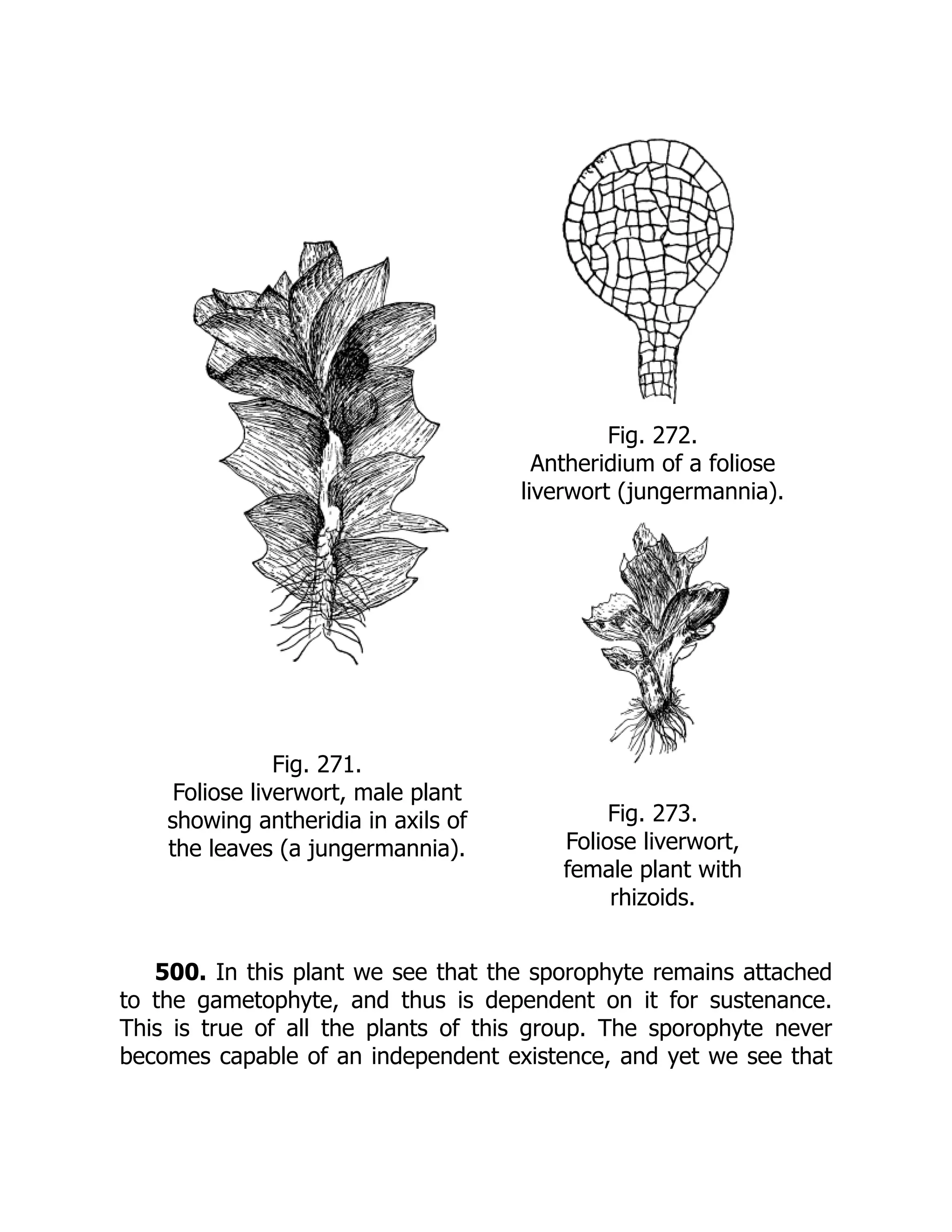

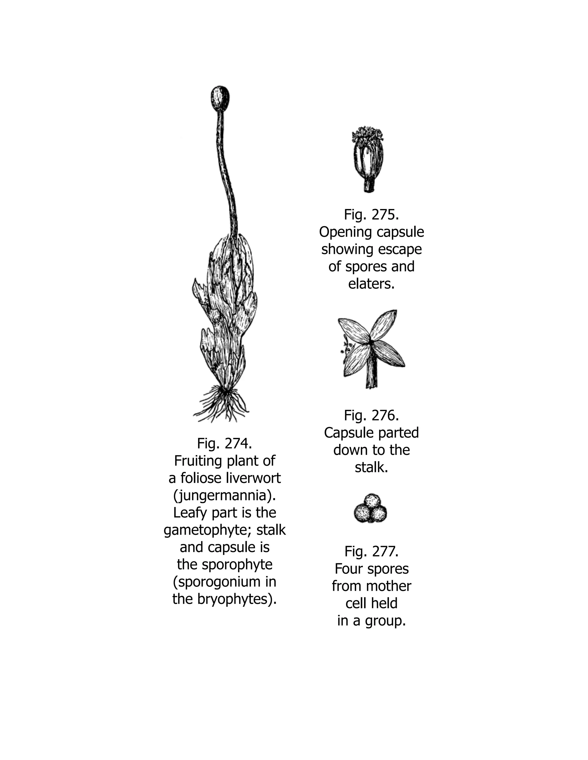
![Fig. 278.
Elaters, at left
showing the two
spiral marks, at
right a branched
elater.
Figs. 275-278.—Sporogonium of liverwort (jungermannia) opening
by splitting into four parts,
showing details of elaters and spores.
The Horned Liverworts.[25]](https://image.slidesharecdn.com/5350-250413224758-767bf818/75/Pro-Data-Visualization-using-R-and-JavaScript-1st-Edition-Tom-Barker-54-2048.jpg)

![the spore-bearing tube is the columella. The cells of the wall contain
chlorophyll, and there are true stomata with guard cells in the
epidermal layer.
508. Spores and elaters.—In the spore-bearing tissue there
are two layers of cells (the archesporium). Each cell is a potential
mother cell. The cells, however, of alternate tiers do not form
spores. They elongate some what and are somewhat irregular and
sometimes divide or branch. They are supposed to represent
rudimentary elaters. The cells in the other tiers are actual mother
cells, and each one forms four spores.
509. The sporophyte of anthoceros represents the highest
type found in the liverworts. The spongy green parenchyma forming
the wall, with the stomata in the epidermal layer, fits this tissue for
the process of photosynthesis, so that this part of the sporophyte
functions as the green leaf of the seed plants. It has been suggested
by some that if the rhizoids on the nourishing foot could only extend
outside and anchor in the soil, the sporophyte of anthoceros could
live an independent existence. But we see that it stops short of that.
Classification of the Liverworts.
CLASS HEPATICÆ.
510. Order Marchantiales.[26] —There are two families
represented in the United States.
Family Ricciaceæ, including Riccia and Ricciocarpus.
Family Marchantiaceæ, including Marchantia, Fegatella (=
Conocephalus), Fimbriaria, Targionia, etc.
511. Order Jungermanniales.[27]—There are two subdivisions
of this order. The Anacrogynæ include chiefly thalloid forms with
continued apical growth, the archegonia back of the apical cell.
Examples: Blasia, Aneura, Pellia, etc.](https://image.slidesharecdn.com/5350-250413224758-767bf818/75/Pro-Data-Visualization-using-R-and-JavaScript-1st-Edition-Tom-Barker-58-2048.jpg)
![The Acrogynæ include chiefly foliose forms, the archegonia
arising from the apical cell and in such cases interrupting apical
growth. Examples: Cephalozia, Frullania, Bazzania, Jungermannia,
Ptilidium, Porella, etc.
CLASS ANTHOCEROTES.
512. The Anthocerotes have formerly been placed with the
Hepaticæ as an order. But because of their wide divergence from the
other liverworts in the development of the sexual organs, and
especially in the structure of the sporophyte, they are now by some
separated as a distinct class. There is one order.
Order Anthocerotales.[28]—This includes one family
(Anthocerotaceæ) with Anthoceros and Notothylas in Europe and
North America, and Dendroceros in the tropics. The latter is
epiphytic.](https://image.slidesharecdn.com/5350-250413224758-767bf818/75/Pro-Data-Visualization-using-R-and-JavaScript-1st-Edition-Tom-Barker-59-2048.jpg)
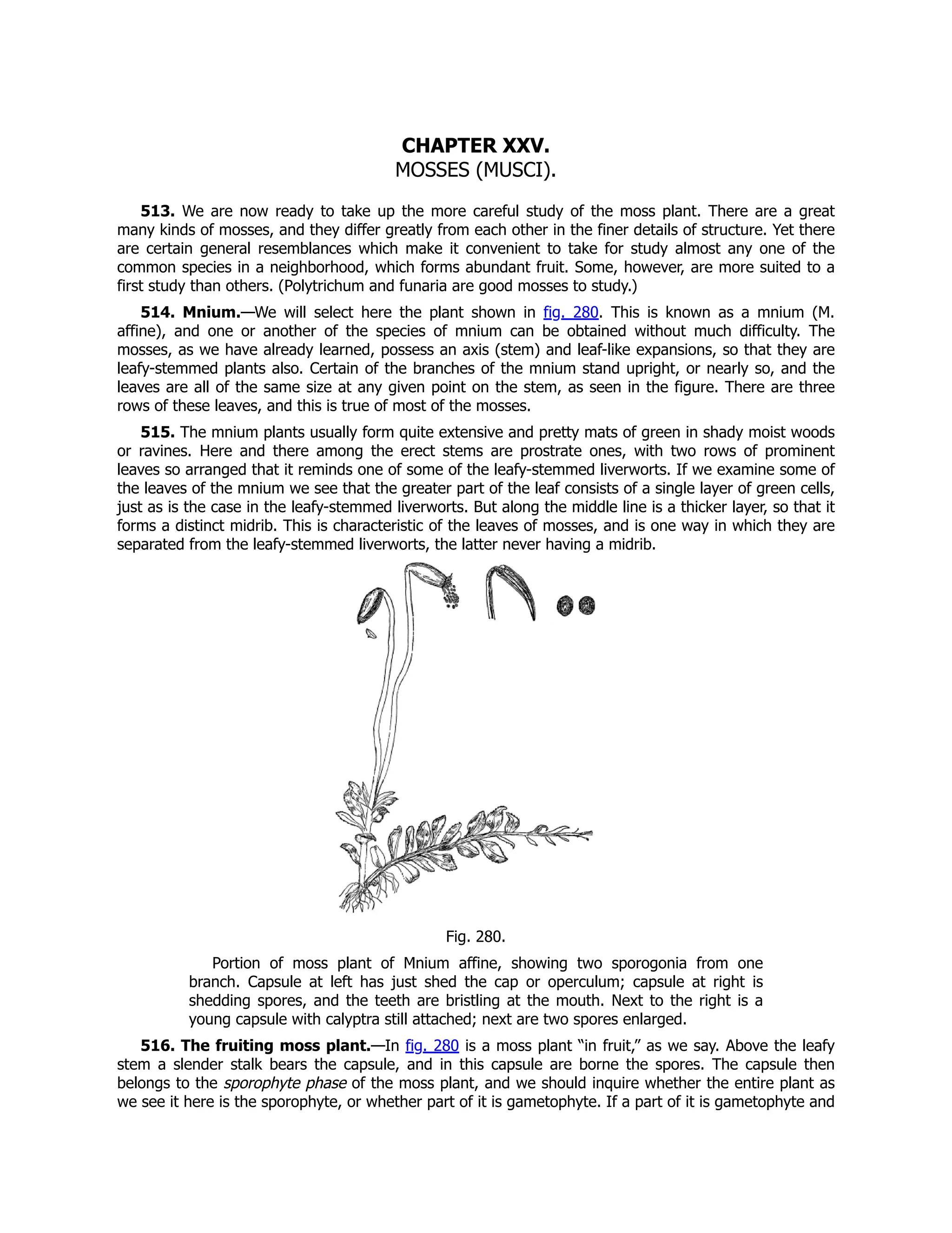
![a part sporophyte, then where does the one end and the other begin? If we strip off the leaves at the
end of the leafy stem, and make a longisection in the middle line, we should find that the stalk which
bears the capsule is simply stuck into the end of the leafy stem, and is not organically connected with it.
This is the dividing line, then, between the gametophyte and the sporophyte. We shall find that here
the archegonium containing the egg is borne, which is a surer way of determining the limits of the two
phases of the plant.
517. The male and female moss plants.—The two plants of mnium shown in figs. 281, 282 are
quite different, as one can easily see, and yet they belong to the same species. One is a female plant,
while the other is a male plant. The sexual organs then in mnium, as in many others of the mosses, are
borne on separate plants. The archegonia are borne at the end of the stem, and are protected by
somewhat narrower leaves which closely overlap and are wrapped together. They are similar to the
archegonia of the liverworts.
Fig. 281.
Female plant (gametophyte) of
a moss (mnium), showing
rhizoids below, and the
tuft of leaves above which
protect the archegonia.
Fig. 282.
Male plant (gametophyte) of
a moss (mnium) showing
rhizoids below and the
antheridia at the center
above surrounded by
the rosette of leaves.
The male plants of mnium are easily selected, since the leaves at the end of the stem form a broad
rosette with the antheridia, and some sterile threads packed closely together in the center. The ends of
the mass of antheridia can be seen with the naked eye, as shown in fig. 282. When the antheridia are
ripe, if we make a section through a cluster, or if we merely tease out some from the end with a needle
in a drop of water on the slide, then prepare for examination with the microscope, we can see the form
of the antheridia. They are somewhat clavate or elliptical in outline, as seen in fig. 284. Between them
there stand short threads composed of several cells containing chlorophyll grains. These are sterile
threads (paraphyses).
518. Sporogonium.—In fig. 280 we see illustrated a sporogonium of mnium, which is of course
developed from the fertilized egg-cell of the archegonium. There is a nearly cylindrical capsule, bent
downward, and supported on a long slender stalk. Upon the capsule is a peculiar cap,[29] shaped like a](https://image.slidesharecdn.com/5350-250413224758-767bf818/75/Pro-Data-Visualization-using-R-and-JavaScript-1st-Edition-Tom-Barker-61-2048.jpg)
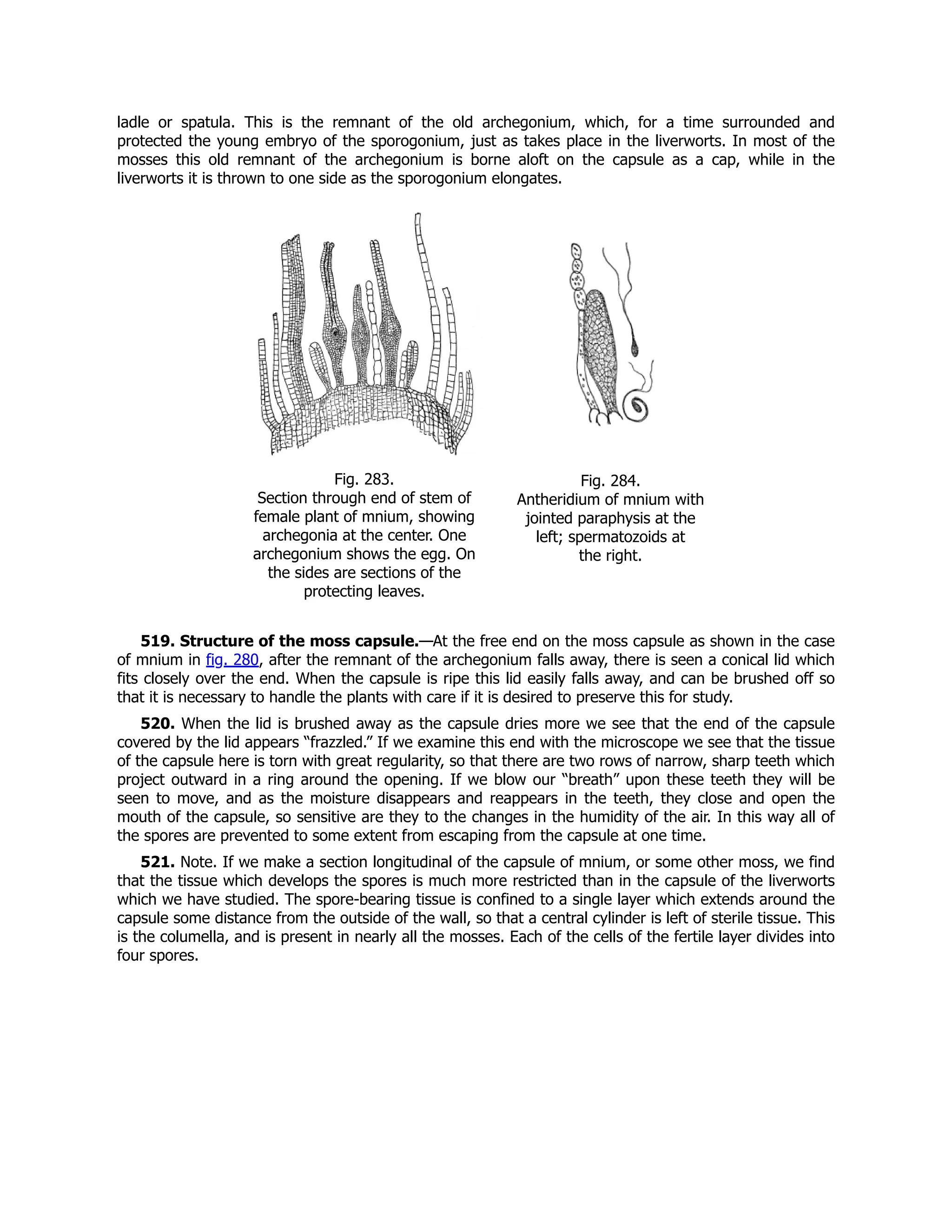
![Fig. 285.
Two different stages of young sporogonium of a moss, still within the
archegonium and wedging their way into the tissue of the end of the stem. h, neck
of archegonium; f, young sporogonium. This shows well the connection of the
sporophyte with the gametophyte.
522. Development of the sporogonium.—The egg-cell after fertilization divides by a wall
crosswise to the axis of the archegonium. Each of these cells continues to divide for a time, so that a
cylinder pointed at both ends is formed. The lower end of this cylinder of tissue wedges its way down
through the base of the archegonium into the tissue of the end of the moss stem as shown in fig. 285.
This forms the foot through which the nutrient materials are passed from the gametophyte to the
sporogonium. The upper part continues to grow, and finally the upper end differentiates into the mature
capsule.
523. Protonema of the moss.—When the spores of a moss germinate they form a thread-like
body, with chlorophyll. This thread becomes branched, and sometimes quite extended tangles of these
threads are formed. This is called the protonema, that is first thread. The older threads become finally
brown, while the later ones are green. From this protonema at certain points buds appear which divide
by close oblique walls. From these buds the leafy stem of the moss plant grows. Threads similar to
these protonemal threads now grow out from the leafy stem, to form the rhizoids. These supply the
moss plant with nutriment, and now the protonema usually dies, though in some few species it persists
for long periods.
Classification of the Mosses.
CLASS MUSCINEÆ (MUSCI).
524. Order Sphagnales.[30]—This order includes the peat mosses. There is but one family
(Sphagnaceæ) and but a single genus (Sphagnum). The peat mosses are widely distributed over the
globe, chiefly occurring in moors, or “bogs,” usually low ground around the shores of lakes, ponds, or
along streams, but they often occur on wet dripping rocks in cool shady places. Small ponds are
sometimes filled in by their growth. As the sphagnum growing in such an abundance of water only
partially decays, “ground” is built up rather rapidly, and the sphagnum remains are known as “peat.”](https://image.slidesharecdn.com/5350-250413224758-767bf818/75/Pro-Data-Visualization-using-R-and-JavaScript-1st-Edition-Tom-Barker-63-2048.jpg)
![This “ground”-building peculiarity of sphagnum sometimes enables the plant (often in conjunction with
others) to fill in ponds completely. (See Atoll Moor, Chapter LV.)
The gametophyte of sphagnum, like that of all the mosses, is dimorphic, but the first part (or
protonema) which develops from the spores is thalloid, and therefore more like the thallose liverworts.
The leafy axis (or gametophore) which develops from the thalloid form is very characteristic (see
Chapter LV).
The archegonia are borne on the free end of the main axis, while the antheridia are borne on short
branches which are brightly colored, red, yellow, etc. The sporophyte (sporogonium) is globose and
possesses a broad foot anchored in the end of a naked prolongation of the end of the leafy
gametophore. This naked prolongation of the gametophore looks like the stalk of the sporogonium, but
a study of its connection with the sporogonium shows that it is part of the gametophyte, which is only
developed after the fertilization of the egg in the archegonium. In the sporogonium there is a short
columella, and the archesporium is in the form of an inverted cup.
525. Order Andreæales.[31]—This order includes the single genus Andreæa. The plants are small
but form extensive mats, growing on rocks in arctic or alpine regions usually. They are sometimes found
in great abundance on bare, rather dry rocks on mountains. The protonema is somewhat thalloid. The
sporogonium opens by splitting longitudinally into four valves. An elongated columella is present so that
the archesporium is shaped like an inverted test tube.
526. Order Archidiales.[32]—This order contains the single genus Archidium, and by some is
placed as an aberrant genus in the Bryales. There is no columella in the simple sporogonium. The
archesporium occupies all the internal part of the sporogonium, some cells being fertile and others
sterile.
527. Order Bryales.[33]—These include the higher mosses, and a very large number of genera and
species. The protonema is filamentous and branched except in a few forms where it is partly thalloid as
in Tetraphis (= Georgia). (Tetraphis pellucida is a common moss on very rotten logs. The capsule has
four prominent teeth.) In a few of the lower genera (Phascum, Pleuridium, etc.) the capsule opens
irregularly, but in the larger number the capsule opens by a lid (operculum). A cylindrical columella is
present, and the archesporium is in the form of a tube open at both ends. (Examples: Polytrichum,
Bryum, Mnium, Hypnum, etc.)
528.
TABLE SHOWING RELATION OF GAMETOPHYTE AND
SPOROPHYTE IN THE LIVERWORTS AND MOSSES.
GAMETOPHYTE.
(Prominent part of the plant.
Leads an independent existence.)
SPOROPHYTE
(Attached to gametophyte
dependent on it for nourishm
Vegetative
Phase
Vegetative
Mulitipl-
ication.
Sexual Organs.
Beginning
of
Sporophyte.
Sterile Part. Fer
Riccia.
Thallus
flattened,
ribbon-like,
forked, or
nearly circular.
Sometimes
by branching
and dying
away of older
parts.
Immersed by surrounding, upward
growth of thallus. Fertilized
egg.
(Develops
sporogonium.)
Wall of
sporogonium,
of one-layer
cells.
C
mass
(arch
deve
Antheridia,
with
spermatozoids.
Archegonia,
with egg in each.
Marchantia.
Thallus
flattened,
ribbon-like,
forked, male
and female
By dying
away of older
parts, and by
gemmæ.
Borne on special receptacles on
different plants.
Fertilized
egg.
(Develops
sporogonium.)
Sterile
part of
stalked is
stalk, wall of
capsule of
several
C
of
(arch
deve
and
Antheridia,
with
spermatozoids,
borne on
Archegonia,
borne on female
gametophore (or](https://image.slidesharecdn.com/5350-250413224758-767bf818/75/Pro-Data-Visualization-using-R-and-JavaScript-1st-Edition-Tom-Barker-64-2048.jpg)
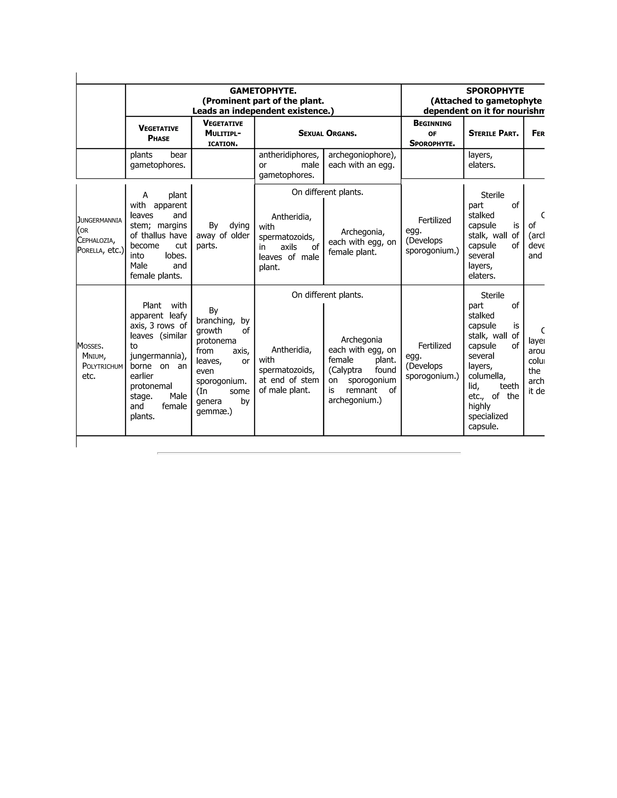

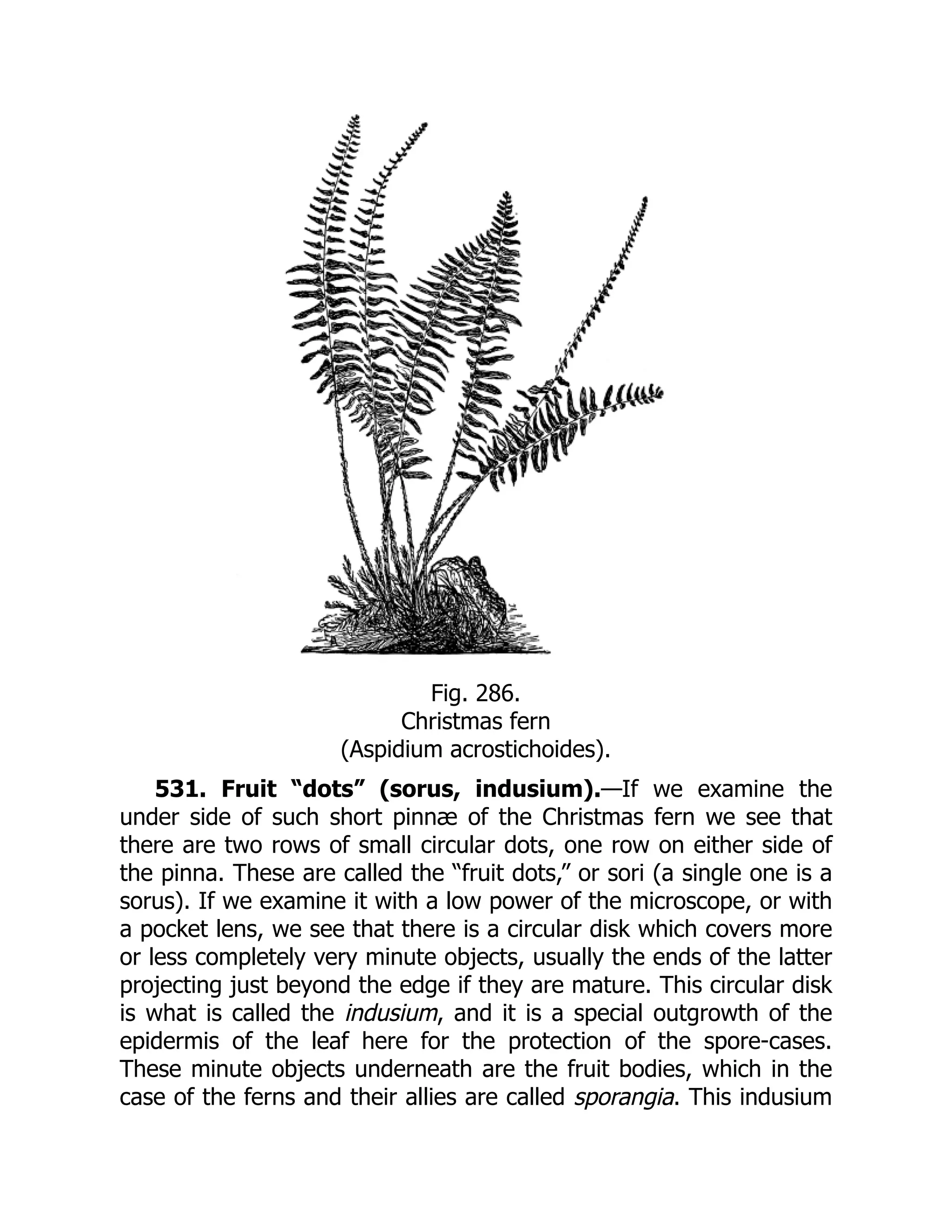
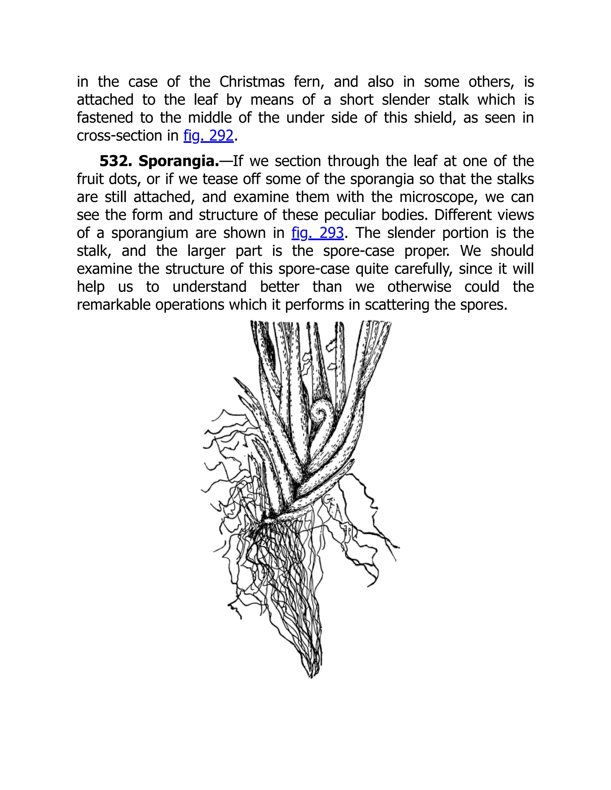
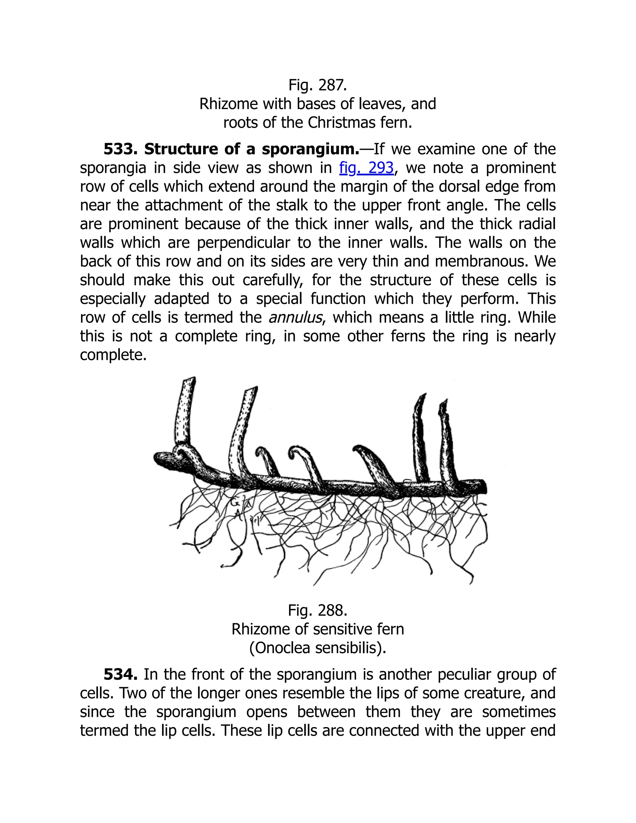
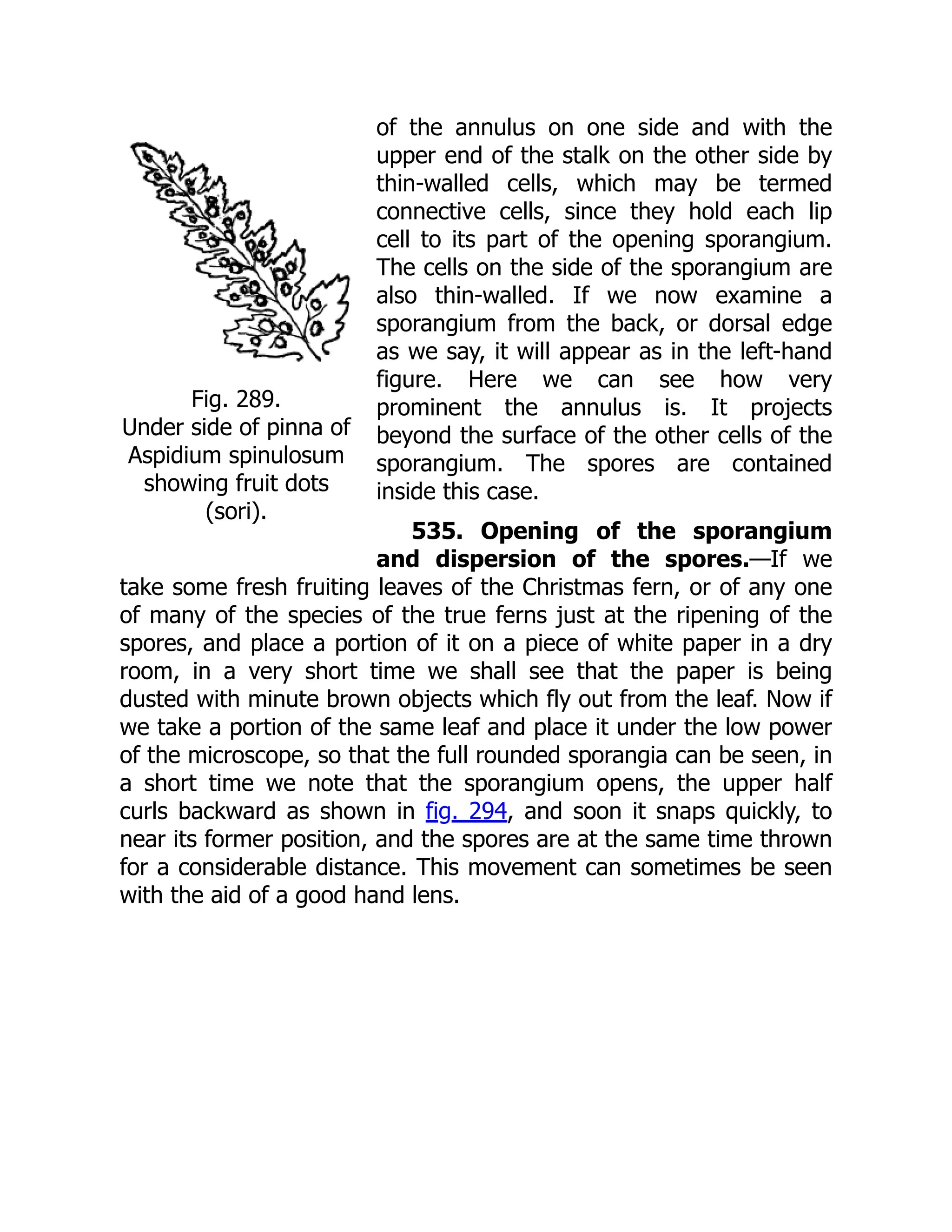
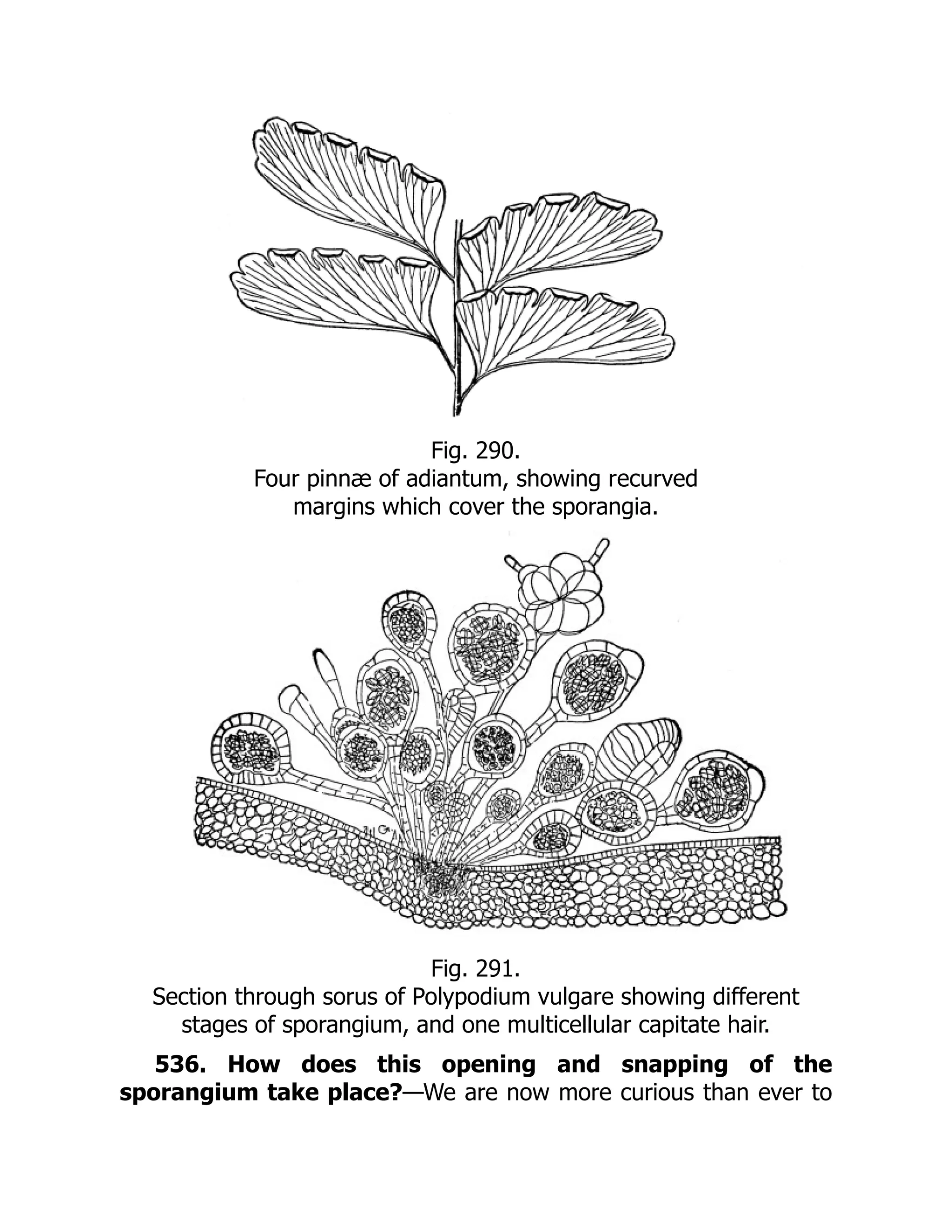
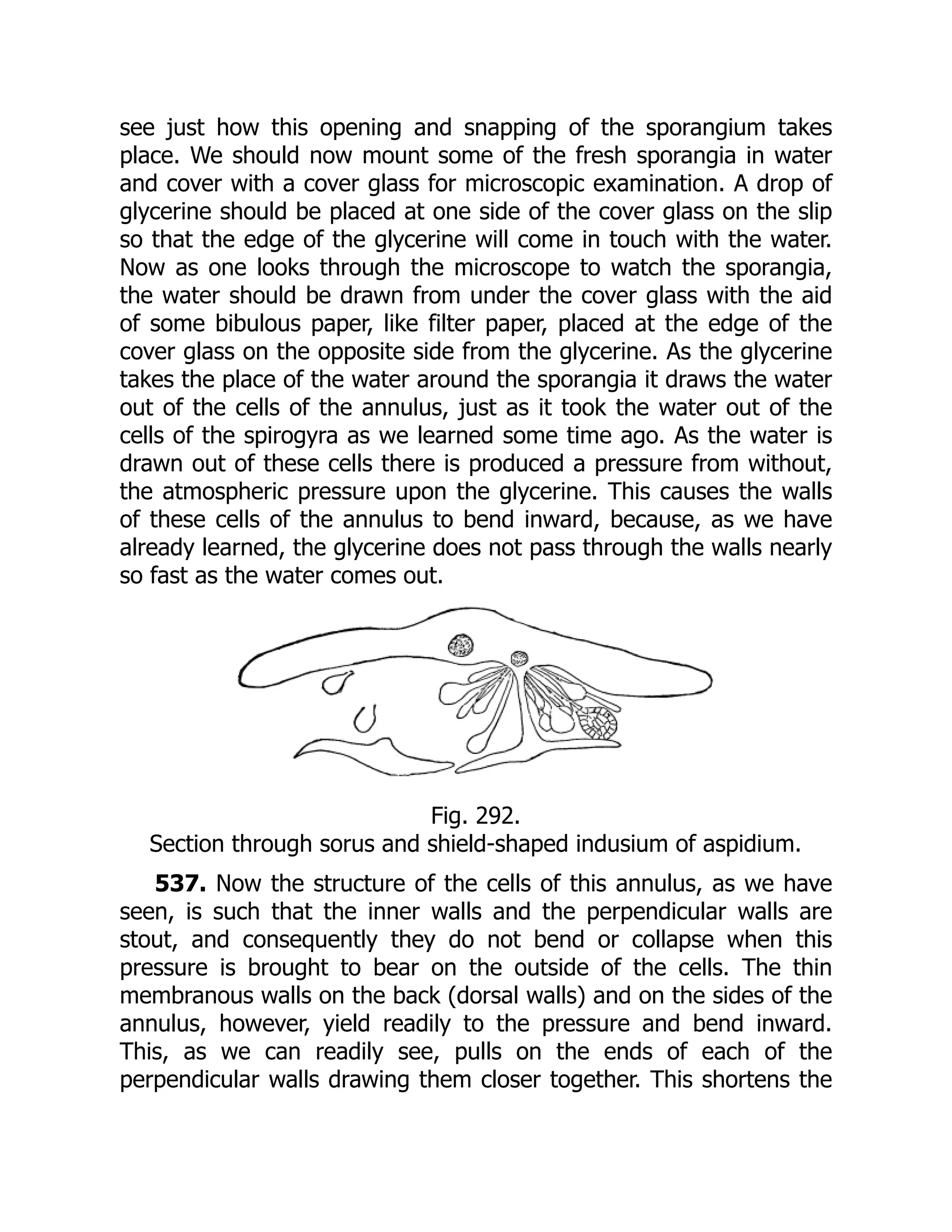
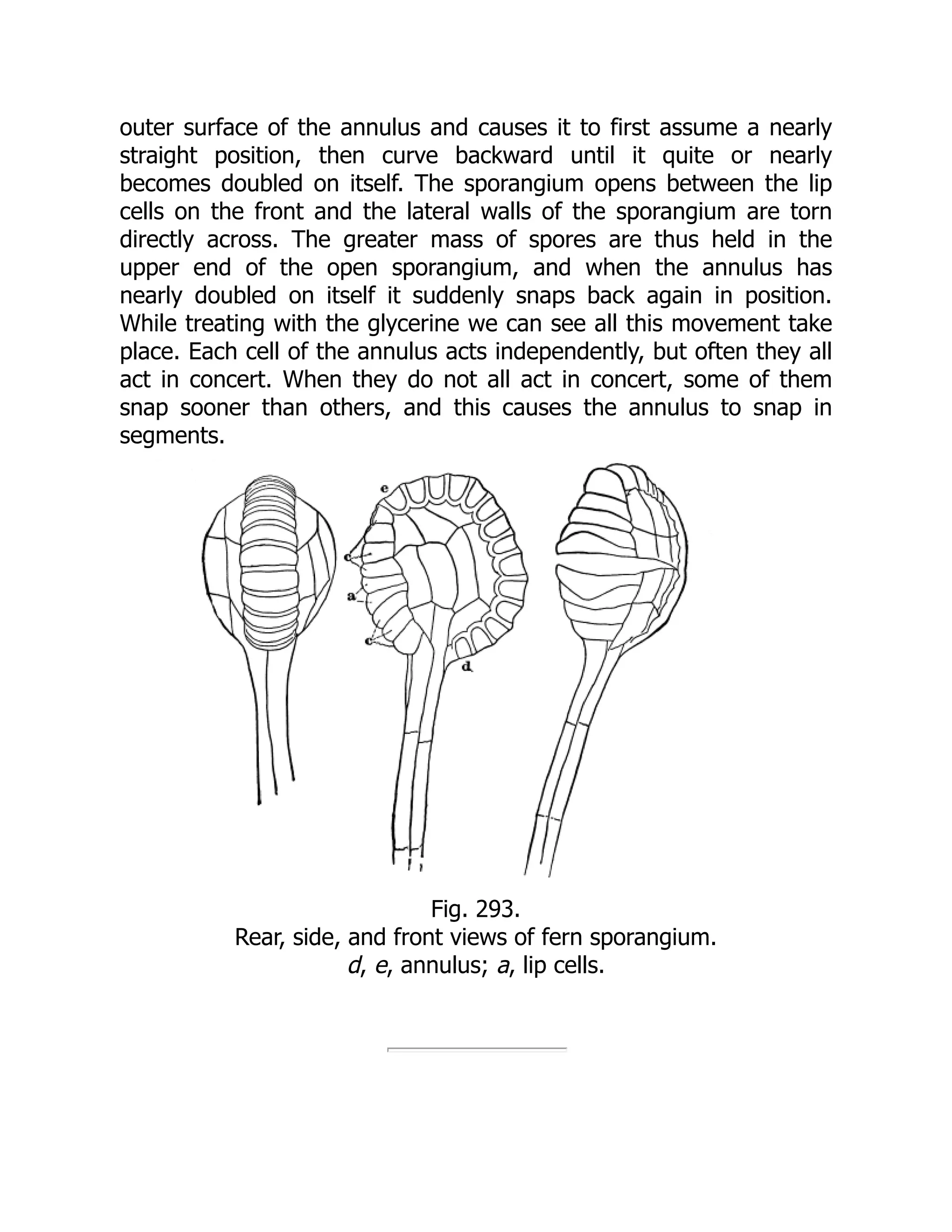
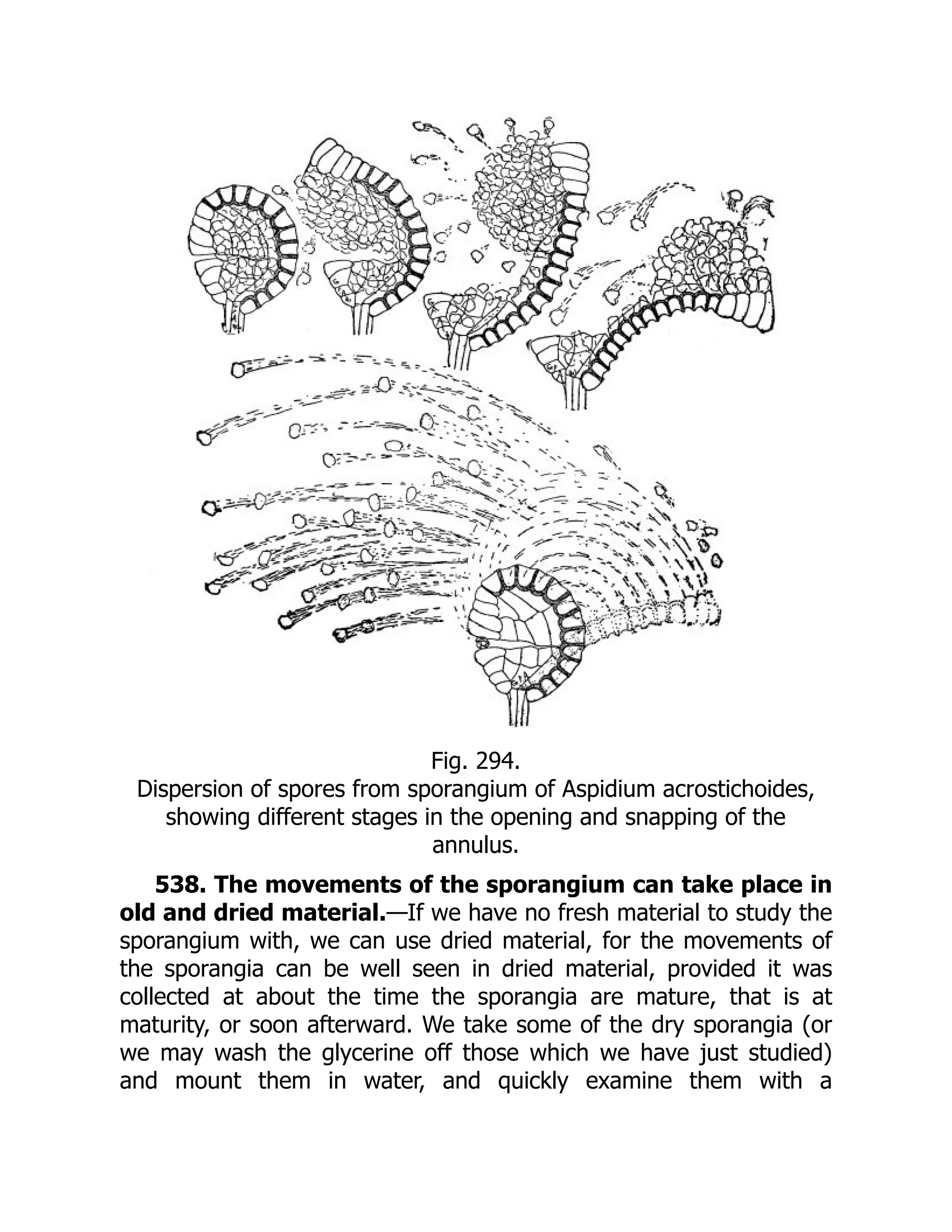


![Chapter 1 ■ Background
10
This chart was created in response to the Fukushima Daiichi nuclear disaster of 2011, and sought to clear up
misinformation and misunderstanding of comparisons being made around the disaster. It did this by demonstrating the
differences in scale for the amount of radiation from sources such as other people or a banana, up to what a fatal dose of
radiation ultimately would be—how all that compared to spending just ten minutes near the Chernobyl meltdown.
Over the last quarter of a century, Edward Tufte, author and professor emeritus at Yale University, has been
working to raise the bar of information graphics. He published groundbreaking books detailing the history of data
visualization, tracing its roots even further back than Playfair, to the beginnings of cartography. Among his principles
is the idea to maximize the amount of information included in each graphic—both by increasing the amount of
variables or data points in a chart and by eliminating the use of what he has coined chartjunk. Chartjunk, according to
Tufte, is anything included in a graph that is not information, including ornamentation or thick, gaudy arrows.
Tufte also invented the sparkline, a time series chart with all axes removed and only the trendline remaining to
show historic variations of a data point without concern for exact context. Sparklines are intended to be small enough
to place in line with a body of text, similar in size to the surrounding characters, and to show the recent or historic
trend of whatever the context of the text is.
Why Data Visualization?
In William Playfair’s introduction to the Commercial and Political Atlas, he rationalizes that just as algebra is the
abbreviated shorthand for arithmetic, so are charts a way to “abbreviate and facilitate the modes of conveying
information from one person to another.” Almost 300 years later, this principle remains the same.
Data visualizations are a universal way to present complex and varied amounts of information, as we saw in our
opening example with the quarterly earnings report. They are also powerful ways to tell a story with data.
Imagine you have your Apache logs in front of you, with thousands of lines all resembling the following:
127.0.0.1 - - [10/Dec/2012:10:39:11 +0300] GET / HTTP/1.1 200 468 - Mozilla/5.0 (X11; U;
Linux i686; en-US; rv:1.8.1.3) Gecko/20061201 Firefox/2.0.0.3 (Ubuntu-feisty)
127.0.0.1 - - [10/Dec/2012:10:39:11 +0300] GET /favicon.ico HTTP/1.1 200 766 - Mozilla/5.0
(X11; U; Linux i686; en-US; rv:1.8.1.3) Gecko/20061201 Firefox/2.0.0.3 (Ubuntu-feisty)
Among other things, we see IP address, date, requested resource, and client user agent. Now imagine this
repeated thousands of times—so many times that your eyes kind of glaze over because each line so closely resembles
the ones around it that it’s hard to discern where each line ends, let alone what cumulative trends exist within.
By using some analysis and visualization tools such as R, or even a commercial product such as Splunk, we can
artfully pull out all kinds of meaningful and interesting stories out of this log, from how often certain HTTP errors occur
and for which resources, to what our most widely used URLs are, to what the geographic distribution of our user base is.
This is just our Apache access log. Imagine casting a wider net, pulling in release information, bugs and
production incidents. What insights we could gather about what we do: from how our velocity impacts our defect
density to how our bugs are distributed across our feature sets. And what better way to communicate those findings
and tell those stories than through a universally digestible medium, like data visualizations?
The point of this book is to explore how we as developers can leverage this practice and medium as part of
continual improvement—both to identify and quantify our successes and opportunities for improvements, and more
effectively communicate our learning and our progress.
Tools
There are a number of excellent tools, environments, and libraries that we can use both to analyze and visualize our
data. The next two sections describe them.](https://crownmelresort.com/image.slidesharecdn.com/5350-250413224758-767bf818/75/Pro-Data-Visualization-using-R-and-JavaScript-1st-Edition-Tom-Barker-17-2048.jpg)


![Chapter 1 ■ Background
15
Creating data visualizations involves four core steps:
1. Identify a problem.
2. Gather the data.
3. Analyze the data.
4. Visualize the data.
Let’s walk through each step in the process and re-create one of the previous charts to demonstrate the process.
Identify a Problem
The very first step is to identify a problem we want to solve. This can be almost anything—from something as
profound and wide-reaching as figuring out why your bug backlog doesn’t seem to go down and stay down, to seeing
what feature releases over a given period in time caused the most production incidents, and why.
For our example, let’s re-create Figure 1-5 and try to quantify the interest in data visualization over time as
represented by the number of New York Times articles on the subject.
Gather Data
We have an idea of what we want to investigate, so let’s dig in. If you are trying to solve a problem or tell a story around
your own product, you would of course start with your own data—maybe your Apache logs, maybe your bug backlog,
maybe exports from your project tracking software.
Note
■
■ If you are focusing on gathering metrics around your product and you don’t already have data handy, you need to
invest in instrumentation.There are many ways to do this, usually by putting logging in your code.At the very least, you want to
log error states and monitor those, but you may want to expand the scope of what you track to include for
debugging purposes
while still respecting both your user’s privacy and your company’s privacy policy. In my book, Pro JavaScript
Performance:
Monitoring and Visualization, I explore ways to track and visualize web and runtime performance.
One important aspect of data gathering is deciding which format your data should be in (if you're lucky) or discovering
which format your data is available in. We’ll next be looking at some of the common data formats in use today.
JSON is an acronym that stands for JavaScript Object Notation. As you probably know, it is essentially a way to
send data as serialized JavaScript objects. We format JSON as follows:
[object]{
[attribute]: [value],
[method] : function(){},
[array]: [item, item]
}
Another way to transfer data is in XML format. XML has an expected syntax, in which elements can have attributes,
which have values, values are always in quotes, and every element must have a closing element. XML looks like this:
parent attribute=value
child attribute=valuenode data/child
/parent
Generally we can expect APIs to return XML or JSON to us, and our preference is usually JSON because as we can
see it is a much more lightweight option just in sheer amount of characters used.](https://crownmelresort.com/image.slidesharecdn.com/5350-250413224758-767bf818/75/Pro-Data-Visualization-using-R-and-JavaScript-1st-Edition-Tom-Barker-22-2048.jpg)

![Chapter 1 ■ Background
17
byline: By AUTHOR,
date: 20121011,
title: TITLE,
url: http://www.nytimes.com/foo.html
}, {
body: BODY COPY,
byline: By AUTHOR,
date: 20121021,
title: TITLE,
url: http://www.nytimes.com/bar.html
}
],
tokens: [
JavaScript
],
total: 2
}
Looking at the high-level JSON structure, we see an attribute named offset, an array named results, an array
named tokens, and another attribute named total. The offset variable is for pagination (what page full of results
we are starting with). The total variable is just what it sounds like: the number of results that are returned for our
query. It’s the results array that we really care about; it is an array of objects, each of which corresponds to an article.
The article objects have attributes named body, byline, date, title, and url.
We now have data that we can begin to look at. That takes us to our next step in the process, analyzing our data.
DATA SCRUBBING
There is often a hidden step here, one that anyone who’s dealt with data knows about: scrubbing the data. Often
the data is either not formatted exactly as we need it or, in even worse cases, it is dirty or incomplete.
In the best-case scenario in which your data just needs to be reformatted or even concatenated, go ahead and do
that, but be sure to not lose the integrity of the data.
Dirty data has fields out of order, fields with obviously bad information in them—think strings in ZIP codes—or
gaps in the data. If your data is dirty, you have several choices:
You could drop the rows in question, but that can harm the integrity of the data—a good example
•
is if you are creating a histogram removing rows could change the distribution and change what
your results will be.
The better alternative is to reach out to whoever administers the source of your data and try and
•
get a better version if it exists.
Whatever the case, if data is dirty or it just needs to be reformatted to be able to be imported into R, expect to
have to scrub your data at some point before you begin your analysis.
Analyze Data
Having data is great, but what does it mean? We determine it through analysis.
Analysis is the most crucial piece of creating data visualizations. It’s only through analysis that we can understand
our data, and it is only through understanding it that we can craft our story to share with others.](https://crownmelresort.com/image.slidesharecdn.com/5350-250413224758-767bf818/75/Pro-Data-Visualization-using-R-and-JavaScript-1st-Edition-Tom-Barker-24-2048.jpg)

![Chapter 1 ■ BaCkground
19
if(length(author) 1){
author - unknown
}
datestamp -paste(month, /, day, /, year, sep=)
datestamp - as.Date(datestamp,%m/%d/%Y)
newrow - data.frame(datestamp, author, title, stringsAsFactors=FALSE, check.rows=FALSE)
df - rbind(df, newrow)
}
rownames(df) - df$datestamp
Note that our example assumes that the data set returned has unique date values. If you get errors with this, you
may need to scrub your returned data set to purge any duplicate rows.
Once our data frame is populated, we can start to do some analysis on the data. Let’s start out by pulling just the
year from every entry, and quickly making a stem and leaf plot to see the shape of the data.
Note John tukey created the stem and leaf plot in his seminal work, Exploratory Data Analysis. Stem and leaf plots
are quick, high-level ways to see the shape of data, much like a histogram. In the stem and leaf plot, we construct the
“stem” column on the left and the “leaf” column on the right. the stem consists of the most significant unique elements
in a result set. the leaf consists of the remainder of the values associated with each stem. In our stem and leaf plot below,
the years are our stem and r shows zeroes for each row associated with a given year. Something else to note is that
often alternating sequential rows are combined into a single row, in the interest of having a more concise visualization.
First, we will create a new variable to hold the year information:
yearlist - as.POSIXlt(df$datestamp)$year+1900
If we inspect this variable, we see that it looks something like this:
yearlist
[1] 2012 2012 2012 2012 2012 2012 2012 2012 2012 2012 2012 2012 2012 2011 2011 2011 2011 2011 2011
2011 2011 2011 2011 2011 2011 2011 2011 2011 2011
[30] 2011 2011 2011 2011 2010 2010 2010 2010 2010 2010 2010 2010 2010 2010 2009 2009 2009 2009 2009
2009 2009 2008 2008 2008 2007 2007 2007 2007 2006
[59] 2006 2006 2006 2005 2005 2005 2005 2005 2005 2004 2003 2003 2003 2002 2002 2002 2002 2001 2001
2000 2000 2000 2000 2000 2000 1999 1999 1999 1999
[88] 1999 1999 1998 1998 1998 1997 1997 1996 1996 1995 1995 1995 1993 1993 1993 1993 1992 1991 1991
1991 1990 1990 1990 1990 1989 1989 1989 1988 1988
[117] 1988 1986 1985 1985 1985 1984 1982 1982 1981
That’s great, that’s exactly what we want: a year to represent every article returned. Next let’s create the stem and
leaf plot:
stem(yearlist)
1980 | 0
1982 | 00
1984 | 0000
1986 | 0
1988 | 000000
Download
from
Wow!
eBook
www.wowebook.com](https://crownmelresort.com/image.slidesharecdn.com/5350-250413224758-767bf818/75/Pro-Data-Visualization-using-R-and-JavaScript-1st-Edition-Tom-Barker-26-2048.jpg)
![Chapter 1 ■ Background
20
1990 | 0000000
1992 | 00000
1994 | 000
1996 | 0000
1998 | 000000000
2000 | 00000000
2002 | 0000000
2004 | 0000000
2006 | 00000000
2008 | 0000000000
2010 | 000000000000000000000000000000
2012 | 0000000000000
Very interesting. We see a gradual build with some dips in the mid-1990s, another gradual build with another dip
in the mid-2000s and a strong explosion since 2010 (the stem and leaf plot groups years together in twos).
Looking at that, my mind starts to envision a story building about a subject growing in popularity. But what
about the authors of these articles? Maybe they are the result of one or two very interested authors that have quite
a bit to say on the subject.
Let’s explore that idea and take a look at the author data that we parsed out. Let’s look at just the unique authors
from our data frame:
length(unique(df$author))
[1] 81
We see that there are 81 unique authors or combination of authors for these articles! Just out of curiosity, let’s take
a look at the breakdown by author for each article. Let’s quickly create a bar chart to see the overall shape of the data
(the bar chart is shown in Figure 1-17):
plot(table(df$author), axes=FALSE)
Figure 1-17. Bar chart of number of articles by author to quickly visualize](https://crownmelresort.com/image.slidesharecdn.com/5350-250413224758-767bf818/75/Pro-Data-Visualization-using-R-and-JavaScript-1st-Edition-Tom-Barker-27-2048.jpg)


![Chapter 2 ■ R Language Primer
29
The Command Line
The R console is where the magic happens! It is a command-line environment where we can run R expressions. The best
way to get up to speed in R is to script in the console, a piece at a time, generally to try out what you’re trying to do, and
tweak it until you get the results that you want. When you finally have a working example, take the code that does what
you want and save it as an R script file.
R script files are just files that contain pure R and can be run in the console using the source command:
source(someRfile.R)
Looking at the preceding code snippet, we assume that the R script lives in the current work directory. The way
we can see what the current work directory is to use the getwd() function:
getwd()
[1] /Users/tomjbarker
We can also set the working directory by using the setwd() function. Note that changes made to the working
directory are not persisted across R sessions unless the session is saved.
setwd(/Users/tomjbarker/Downloads)
getwd()
[1] /Users/tomjbarker/Downloads
Command History
The R console stores commands that you enter and you can cycle through previous commands by pressing the up
arrow. Hit the escape button to return to the command prompt. We can see the history in a separate window pane
by clicking the Show/Hide Command History button at the top of the console. The Show/Hide Command History
button is the rectangle icon with alternating stripes of yellow and green. See Figure 2-5 for the R console with the
command history shown.](https://crownmelresort.com/image.slidesharecdn.com/5350-250413224758-767bf818/75/Pro-Data-Visualization-using-R-and-JavaScript-1st-Edition-Tom-Barker-35-2048.jpg)

![Chapter 2 ■ R Language Primer
31
Packages
Speaking of packages, what are they, exactly? Packages are collections of functions, data sets, or objects that can
be imported into the current session or workspace to extend what we can do in R. Anyone can make a package
and distribute it.
To install a package, we simply type this:
install.packages([package name])
For example, if we want to install the ggplot2 package—which is a widely used and very handy charting
package—we simply type this into the console:
install.packages(ggplot2)
We are immediately prompted to choose the mirror location that we want to use, usually the one closest to our
current location. From there, the install begins. We can see the results in Figure 2-7.
Figure 2-6. Help search results window](https://crownmelresort.com/image.slidesharecdn.com/5350-250413224758-767bf818/75/Pro-Data-Visualization-using-R-and-JavaScript-1st-Edition-Tom-Barker-37-2048.jpg)

![Chapter 2 ■ R Language Primer
33
codetools Code Analysis Tools for R
colorspace Color Space Manipulation
compiler The R Compiler Package
datasets The R Datasets Package
dichromat Color schemes for dichromats
digest Create cryptographic hash digests of R objects
foreign Read Data Stored by Minitab, S, SAS, SPSS, Stata, Systat, dBase,
...
ggplot2 An implementation of the Grammar of Graphics
gpairs gpairs: The Generalized Pairs Plot
graphics The R Graphics Package
grDevices The R Graphics Devices and Support for Colours and Fonts
grid The Grid Graphics Package
gtable Arrange grobs in tables.
KernSmooth Functions for kernel smoothing for Wand Jones (1995)
labeling Axis Labeling
lattice Lattice Graphics
mapdata Extra Map Databases
mapproj Map Projections
maps Draw Geographical Maps
Importing Data
So now our environment is downloaded and installed, and we know how to install any packages that we may need.
Now we can begin using R.
The first thing we’ll normally want to do is import your data. There are several ways to import data, but the most
common way is to use the read() function, which has several flavors:
read.table([file to read])
read.csv([file to read])
To see this in action, let’s first create a text file named temptext.txt that is formatted like so:
134,432,435,313,11
403,200,500,404,33
77,321,90,2002,395
We can read this into a variable that we will name temptxt:
temptxt - read.table(temptext.txt)
Notice that as we are assigning value to this variable, we are not using an equal sign as the assignment operator.
We are instead using an arrow -. That is R’s assignment operator, although it does also support the equal sign if you
are so inclined. But the standard is the arrow, and all examples that we will show in this book will use the arrow.
If we print out the temptxt variable, we see that it is structured as follows:
temptxt
V1
1 134,432,435,313,11
2 403,200,500,404,33
3 77,321,90,2002,395](https://crownmelresort.com/image.slidesharecdn.com/5350-250413224758-767bf818/75/Pro-Data-Visualization-using-R-and-JavaScript-1st-Edition-Tom-Barker-39-2048.jpg)
![Chapter 2 ■ R Language Primer
34
We see that our variable is a table-like structure called a data frame, and R has assigned a column name (V1) and
row IDs to our data structure. More on column names soon.
The read() function has a number of parameters that you can use to refine how the data is imported and
formatted once it is imported.
Using Headers
The header parameter tells R to treat the first line in the external file as containing header information. The first line
then becomes the column names of the data frame.
For example, suppose we have a log file structured like this:
url, day, date, loadtime, bytes, httprequests, loadtime_repeatview
http://apress.com, Sun, 01 Jul 2012 14:01:28 +0000,7042,956680,73,3341
http://apress.com, Sun, 01 Jul 2012 14:01:31 +0000,6932,892902,76,3428
http://apress.com, Sun, 01 Jul 2012 14:01:33 +0000,4157,594908,38,1614
We can load it into a variable named wpo like so:
wpo - read.table(wpo.txt, header=TRUE)
wpo
url day date loadtime bytes httprequests loadtime_repeatview
1 http://apress.com,Sun,1 Jul 2012 14:01:28 +0000,7042,955550,73,3191
2 http://apress.com,Sun,1 Jul 2012 14:01:31 +0000,6932,892442,76,3728
3 http://apress.com,Sun,1 Jul 2012 14:01:33 +0000,4157,614908,38,1514
When we call the colnames() function to see what the column names are for wpo, we see the following:
colnames(wpo)
[1] url day date loadtime
[5] bytes httprequests loadtime_repeatview
Specifying a String Delimiter
The sep attribute tells the read() function what to use as the string delimiter for parsing the columns in the external
data file. In all the examples we’ve looked at so far, commas are our delimiters, but we could use instead pipes | or any
other character that we want.
Say, for example, that our previous temptxt example used pipes; we would just update the code to be as follows:
134|432|435|313|11
403|200|500|404|33
77|321|90|2002|395
temptxt - read.table(temptext.txt, sep=|)
temptxt
V1 V2 V3 V4 V5
1 134 432 435 313 11
2 403 200 500 404 33
3 77 321 90 2002 395
Oh, notice that? We actually got distinct column names this time (V1, V2, V3, V4, V5). Before, we didn’t specify a
delimiter, so R assumed that each row was one big blob of text and lumped it into a single column (V1).](https://crownmelresort.com/image.slidesharecdn.com/5350-250413224758-767bf818/75/Pro-Data-Visualization-using-R-and-JavaScript-1st-Edition-Tom-Barker-40-2048.jpg)

![Chapter 2 ■ R Language Primer
36
Data types in R are called modes, and can be the following:
numeric
•
character
•
logical
•
complex
•
raw
•
list
•
We can use the mode() function to check the mode of a variable.
Character and numeric modes correspond to string and number (both integer and float) data types. Logical
modes are Boolean values.
n - 122132
mode(n)
[1] numeric
c - test text
mode(c)
[1] character
l - TRUE
mode(l)
[1] logical
We can perform string concatenation using the paste() function. We can use the substr() function to pull
characters out of strings. Let’s look at some examples in code.
Usually, I keep a list of directories that I either read data from or write charts to. Then when I want to reference
a new data file that exists in the data directory, I will just append the new file name to the data directory:
dataDirectory - /Users/tomjbarker/org/data/
buglist - paste(dataDirectory, bugs.txt, sep=)
buglist
[1] /Users/tomjbarker/org/data/bugs.txt
The paste() function takes N amount of strings and concatenates them together. It accepts an argument named
sep that allows us to specify a string that we can use to be a delimiter between joined strings. We don’t want anything
separating our joined strings that we pass in an empty string.
If we want to pull characters from a string, we use the substr() function. The substr() function takes a string to
parse, a starting location, and a stopping location. It returns all the character inclusively from the starting location up
to the ending location. (Remember that in R, lists are not 0-based like most other languages, but instead have
a starting index of 1.)
substr(test, 1,2)
[1] te
In the preceding example, we pass in the string “test” and tell the substr() function to return the first and
second characters.
Complex mode is for complex numbers. The raw mode is to store raw byte data.](https://crownmelresort.com/image.slidesharecdn.com/5350-250413224758-767bf818/75/Pro-Data-Visualization-using-R-and-JavaScript-1st-Edition-Tom-Barker-42-2048.jpg)
![Chapter 2 ■ R Language Primer
37
List data types or modes can be one of three classes: vectors, matrices, or data frames. If we call mode() for vectors
or matrices, they return the mode of the data that they contain; class() returns the class. If we call mode() on a data
frame, it returns the type list:
v - c(1:10)
mode(v)
[1] numeric
m - matrix(c(1:10), byrow=TRUE)
mode(m)
[1] numeric
class(m)
[1] matrix
d - data.frame(c(1:10))
mode(d)
[1] list
class(d)
[1] data.frame
Note that we just typed 1:10 rather than the whole sequence of numbers between 1 and 10:
v - c(1:10)
Vectors are single-dimensional arrays that can hold only values of a single mode at a time. It’s when we get to
data frames and matrices that R really starts to get interesting. The next two sections cover those classes.
Data Frames
We saw at the beginning of this chapter that the read() function takes in external data and saves it as a data frame.
Data frames are like arrays in most other loosely typed languages: they are containers that hold different types of data,
referenced by index. The main thing to realize, though, is that data frames see the data that they contain as rows, columns,
and combinations of the two.
For example, think of a data frame as formatted as follows:
col col col col col
row [ 1 ] [ 1 ] [ 1 ] [ 1 ] [ 1 ]
row [ 1 ] [ 1 ] [ 1 ] [ 1 ] [ 1 ]
row [ 1 ] [ 1 ] [ 1 ] [ 1 ] [ 1 ]
row [ 1 ] [ 1 ] [ 1 ] [ 1 ] [ 1 ]
If we try to reference the first index in the preceding data frame as we traditionally would with an array, say
dataframe[1], R would instead return the first column of data, not the first item. So data frames are referenced by their
column and row. So dataframe[1] returns the first column and dataframe[,2] returns the first row.
Let’s demonstrate this in code.
First let’s create some vectors using the combine function, c(). Remember that vectors are collections of data all
of the same type. The combine function takes a series of values and combines them into vectors.
col1 - c(1,2,3,4,5,6,7,8)
col2 - c(1,2,3,4,5,6,7,8)
col3 - c(1,2,3,4,5,6,7,8)
col4 - c(1,2,3,4,5,6,7,8)](https://crownmelresort.com/image.slidesharecdn.com/5350-250413224758-767bf818/75/Pro-Data-Visualization-using-R-and-JavaScript-1st-Edition-Tom-Barker-43-2048.jpg)
![Chapter 2 ■ R Language Primer
38
Then let’s combine these vectors into a data frame:
df - data.frame(col1,col2,col3,col4)
Now let’s print the data frame to see the contents and the structure of it:
df
col1 col2 col3 col4
1 1 1 1 1
2 2 2 2 2
3 3 3 3 3
4 4 4 4 4
5 5 5 5 5
6 6 6 6 6
7 7 7 7 7
8 8 8 8 8
Notice that it took each vector and made each one a column. Also notice that each row has an ID; by default,
it is a number, but we can override that.
If we reference the first index, we see that the data frame returns the first column:
df[1]
col1
1 1
2 2
3 3
4 4
5 5
6 6
7 7
8 8
If we put a comma in front of that 1, we reference the first row:
df[,1]
[1] 1 2 3 4 5 6 7 8
So accessing contents of a data frame is done by specifying [column, row].
Matrices work much the same way.
Matrices
Matrices are just like data frames in that they contain rows and columns and can be referenced by either. The core
difference between the two is that data frames can hold different data types but matrices can hold only one type of data.
This presents a philosophical difference. Usually you use data frames to hold data read in externally, like from a
flat file or a database because those are generally of mixed type. You normally store data in matrices that you want to
apply functions to (more on applying functions to lists in a little bit).](https://crownmelresort.com/image.slidesharecdn.com/5350-250413224758-767bf818/75/Pro-Data-Visualization-using-R-and-JavaScript-1st-Edition-Tom-Barker-44-2048.jpg)
![Chapter 2 ■ R Language Primer
39
To create a matrix, we must use the matrix() function, pass in a vector, and tell the function how to distribute
the vector:
The
• nrow parameter specifies how many rows the matrix should have
The
• ncol parameter specifies the number of columns.
The
• byrow parameter tells R that the contents of the vector should be distributed by iterating
across rows if TRUE or by columns if FALSE.
content - c(1,2,3,4,5,6,7,8,9,10)
m1 - matrix(content, nrow=2, ncol=5, byrow=TRUE)
m1
[,1] [,2] [,3] [,4] [,5]
[1,] 1 2 3 4 5
[2,] 6 7 8 9 10
Notice that in the previous example that the m1 matrix is filled in horizontally, row by row. In the following
example, the m1 matrix is filled in vertically by column:
content - c(1,2,3,4,5,6,7,8,9,10)
m1 - matrix(content, nrow=2, ncol=5, byrow=FALSE)
m1
[,1] [,2] [,3] [,4] [,5]
[1,] 1 3 5 7 9
[2,] 2 4 6 8 10
Remember that instead of manually typing out all the numbers in the previous content vector, if the numbers are
a sequence we can just type this:
content - (1:10)
We reference the content in matrices with the square bracket, specifying the row and column, respectively.
m1[1,4]
[1] 7
We can convert a data frame to a matrix if the data frame contains only a single type of data. To do this we use the
as.matrix() function. Often times we will do this when passing a data frame to a plotting function to draw a chart.
barplot(as.matrix(df))
Below we create a data frame called df. We populate the data frame with ten consecutive numbers. We then use
as.matrix() to convert df into a matrix and save the result into a new variable called m:
df - data.frame(1:10)
df
X1.10
1 1
2 2
3 3](https://crownmelresort.com/image.slidesharecdn.com/5350-250413224758-767bf818/75/Pro-Data-Visualization-using-R-and-JavaScript-1st-Edition-Tom-Barker-45-2048.jpg)
![Chapter 2 ■ r Language primer
40
4 4
5 5
6 6
7 7
8 8
9 9
10 10
class(df)
[1] data.frame
m - as.matrix(df)
class(m)
[1] matrix
Keep in mind that because they are all the same data type, matrices require less overhead and are intrinsically
more efficient than data frames. If we compare the size of our matrix m and our data frame df, we see that with just ten
items there is a size difference.
object.size(m)
312 bytes
object.size(df)
440 bytes
With that said, if we increase the scale of this, the increase in efficiency does not equally scale. Compare the following:
big_df - data.frame(1:40000000)
big_m - matrix(1:40000000)
object.size(big_m)
160000112 bytes
object.size(big_df)
160000400 bytes
We can see that the first example with the small data set showed that the matrix was 30 percent smaller in size
than the data frame, but at the larger scale in the second example the matrix was only .00018 percent smaller than
the data frame.
Adding Lists
When combining or adding to data frames or matrices, you generally add either by the row or the column using
rbind() or cbind().
To demonstrate this, let’s add a new row to our data frame df. We’ll pass df into rbind() along with the new row
to add to df. The new row contains just one element, the number 11:
df - rbind(df, 11)
df
X1.10
1 1
2 2
3 3
4 4
5 5
6 6
Download
from
Wow!
eBook
www.wowebook.com](https://crownmelresort.com/image.slidesharecdn.com/5350-250413224758-767bf818/75/Pro-Data-Visualization-using-R-and-JavaScript-1st-Edition-Tom-Barker-46-2048.jpg)
![Chapter 2 ■ R Language Primer
41
7 7
8 8
9 9
10 10
11 11
Now let’s add a new column to our matrix m. To do this, we simply pass m into cbind() as the first parameter;
the second parameter is a new matrix that will be appended to the new column.
m - rbind(m, 11)
m - cbind(m, matrix(c(50:60), byrow=FALSE))
m
X1.10
[1,] 1 50
[2,] 2 51
[3,] 3 52
[4,] 4 53
[5,] 5 54
[6,] 6 55
[7,] 7 56
[8,] 8 57
[9,] 9 58
[10,] 10 59
[11,] 11 60
What about vectors, you may ask? Well, let’s look at adding to our content vector. We simply use the combine
function to combine the current vector with a new vector:
content - c(1,2,3,4,5,6,7,8,9,10)
content - c(content, c(11:20))
content
[1] 1 2 3 4 5 6 7 8 9 10 11 12 13 14 15 16 17 18 19 20
Looping Through Lists
As developers who generally work in procedural languages, or at least came up the ranks using procedural languages
(though in recent years functional programming paradigms have become much more mainstream), we’re most
likely used to looping through our arrays when we want to process the data within them. This is in contrast to purely
functional languages where we would instead apply a function to our lists, like the map() function. R supports both
paradigms. Let’s first look at how to loop through our lists.
The most useful loop that R supports is the for in loop. The basic structure of a for in loop can be seen here:.
for(i in 1:5){print(i)}
[1] 1
[1] 2
[1] 3
[1] 4
[1] 5](https://crownmelresort.com/image.slidesharecdn.com/5350-250413224758-767bf818/75/Pro-Data-Visualization-using-R-and-JavaScript-1st-Edition-Tom-Barker-47-2048.jpg)
![Chapter 2 ■ R Language Primer
42
The variable i increments in value each step through the iteration. We can use the for in loop to step through
lists. We can specify a particular column to iterate through, like the following, in which we loop through the X1.10
column of the data frame df.
for(n in df$X1.10){ print(n)}
[1] 1
[1] 2
[1] 3
[1] 4
[1] 5
[1] 6
[1] 7
[1] 8
[1] 9
[1] 10
[1] 11
Note that we are accessing the columns of data frames via the dollar sign operator. The general pattern is
[data frame]$[column name].
Applying Functions to Lists
But the way that R really wants to be used is to apply functions to the contents of lists (see Figure 2-8).
function
element
element
element
element
Figure 2-8. Apply a function to list elements
We do this in R with the apply() function.](https://crownmelresort.com/image.slidesharecdn.com/5350-250413224758-767bf818/75/Pro-Data-Visualization-using-R-and-JavaScript-1st-Edition-Tom-Barker-48-2048.jpg)
![Chapter 2 ■ R Language Primer
43
The apply() function takes several parameters:
First is our list.
•
Next a number vector to indicate how we apply the function through the list (
• 1 is for rows, 2 is
for columns, and c[1,2] indicates both rows and columns).
Finally is the function to apply to the list:
•
apply([list], [how to apply function], [function to apply])
Let’s look at an example. Let’s make a new matrix that we’ll call m. The matrix m will have ten columns and four rows:
m - matrix(c(1:40), byrow=FALSE, ncol=10)
m
[,1] [,2] [,3] [,4] [,5] [,6] [,7] [,8] [,9] [,10]
[1,] 1 5 9 13 17 21 25 29 33 37
[2,] 2 6 10 14 18 22 26 30 34 38
[3,] 3 7 11 15 19 23 27 31 35 39
[4,] 4 8 12 16 20 24 28 32 36 40
Now say we wanted to increment every number in the m matrix. We could simply use apply() as follows:
apply(m, 2, function(x) x - x + 1)
[,1] [,2] [,3] [,4] [,5] [,6] [,7] [,8] [,9] [,10]
[1,] 2 6 10 14 18 22 26 30 34 38
[2,] 3 7 11 15 19 23 27 31 35 39
[3,] 4 8 12 16 20 24 28 32 36 40
[4,] 5 9 13 17 21 25 29 33 37 41
Do you see what we did there? We passed in m, we specified that we wanted to apply the function across the
columns, and finally we passed in an anonymous function. The function accepts a parameter that we called x.
The parameter x is a reference to the current matrix element. From there, we just increment the value of x by 1.
OK, say we wanted to do something slightly more interesting, such as zeroing out all the even numbers in the
matrix. We could do the following:
apply(m,c(1,2),function(x){if((x %% 2) == 0) x - 0 else x - x})
[,1] [,2] [,3] [,4] [,5] [,6] [,7] [,8] [,9] [,10]
[1,] 1 5 9 13 17 21 25 29 33 37
[2,] 0 0 0 0 0 0 0 0 0 0
[3,] 3 7 11 15 19 23 27 31 35 39
[4,] 0 0 0 0 0 0 0 0 0 0
For the sake of clarity let’s break out that function that we are applying. We simply check to see whether the
current element is even by checking to see whether it has a remainder when divided by two. If it is, we set it to zero;
if it isn’t, we set it to itself:
function(x){
if((x %% 2) == 0)
x - 0
else
x - x
}](https://crownmelresort.com/image.slidesharecdn.com/5350-250413224758-767bf818/75/Pro-Data-Visualization-using-R-and-JavaScript-1st-Edition-Tom-Barker-49-2048.jpg)


![Fig. 278.
Elaters, at left
showing the two
spiral marks, at
right a branched
elater.
Figs. 275-278.—Sporogonium of liverwort (jungermannia) opening
by splitting into four parts,
showing details of elaters and spores.
The Horned Liverworts.[25]](https://crownmelresort.com/image.slidesharecdn.com/5350-250413224758-767bf818/75/Pro-Data-Visualization-using-R-and-JavaScript-1st-Edition-Tom-Barker-54-2048.jpg)


![the spore-bearing tube is the columella. The cells of the wall contain
chlorophyll, and there are true stomata with guard cells in the
epidermal layer.
508. Spores and elaters.—In the spore-bearing tissue there
are two layers of cells (the archesporium). Each cell is a potential
mother cell. The cells, however, of alternate tiers do not form
spores. They elongate some what and are somewhat irregular and
sometimes divide or branch. They are supposed to represent
rudimentary elaters. The cells in the other tiers are actual mother
cells, and each one forms four spores.
509. The sporophyte of anthoceros represents the highest
type found in the liverworts. The spongy green parenchyma forming
the wall, with the stomata in the epidermal layer, fits this tissue for
the process of photosynthesis, so that this part of the sporophyte
functions as the green leaf of the seed plants. It has been suggested
by some that if the rhizoids on the nourishing foot could only extend
outside and anchor in the soil, the sporophyte of anthoceros could
live an independent existence. But we see that it stops short of that.
Classification of the Liverworts.
CLASS HEPATICÆ.
510. Order Marchantiales.[26] —There are two families
represented in the United States.
Family Ricciaceæ, including Riccia and Ricciocarpus.
Family Marchantiaceæ, including Marchantia, Fegatella (=
Conocephalus), Fimbriaria, Targionia, etc.
511. Order Jungermanniales.[27]—There are two subdivisions
of this order. The Anacrogynæ include chiefly thalloid forms with
continued apical growth, the archegonia back of the apical cell.
Examples: Blasia, Aneura, Pellia, etc.](https://crownmelresort.com/image.slidesharecdn.com/5350-250413224758-767bf818/75/Pro-Data-Visualization-using-R-and-JavaScript-1st-Edition-Tom-Barker-58-2048.jpg)
![The Acrogynæ include chiefly foliose forms, the archegonia
arising from the apical cell and in such cases interrupting apical
growth. Examples: Cephalozia, Frullania, Bazzania, Jungermannia,
Ptilidium, Porella, etc.
CLASS ANTHOCEROTES.
512. The Anthocerotes have formerly been placed with the
Hepaticæ as an order. But because of their wide divergence from the
other liverworts in the development of the sexual organs, and
especially in the structure of the sporophyte, they are now by some
separated as a distinct class. There is one order.
Order Anthocerotales.[28]—This includes one family
(Anthocerotaceæ) with Anthoceros and Notothylas in Europe and
North America, and Dendroceros in the tropics. The latter is
epiphytic.](https://crownmelresort.com/image.slidesharecdn.com/5350-250413224758-767bf818/75/Pro-Data-Visualization-using-R-and-JavaScript-1st-Edition-Tom-Barker-59-2048.jpg)

![a part sporophyte, then where does the one end and the other begin? If we strip off the leaves at the
end of the leafy stem, and make a longisection in the middle line, we should find that the stalk which
bears the capsule is simply stuck into the end of the leafy stem, and is not organically connected with it.
This is the dividing line, then, between the gametophyte and the sporophyte. We shall find that here
the archegonium containing the egg is borne, which is a surer way of determining the limits of the two
phases of the plant.
517. The male and female moss plants.—The two plants of mnium shown in figs. 281, 282 are
quite different, as one can easily see, and yet they belong to the same species. One is a female plant,
while the other is a male plant. The sexual organs then in mnium, as in many others of the mosses, are
borne on separate plants. The archegonia are borne at the end of the stem, and are protected by
somewhat narrower leaves which closely overlap and are wrapped together. They are similar to the
archegonia of the liverworts.
Fig. 281.
Female plant (gametophyte) of
a moss (mnium), showing
rhizoids below, and the
tuft of leaves above which
protect the archegonia.
Fig. 282.
Male plant (gametophyte) of
a moss (mnium) showing
rhizoids below and the
antheridia at the center
above surrounded by
the rosette of leaves.
The male plants of mnium are easily selected, since the leaves at the end of the stem form a broad
rosette with the antheridia, and some sterile threads packed closely together in the center. The ends of
the mass of antheridia can be seen with the naked eye, as shown in fig. 282. When the antheridia are
ripe, if we make a section through a cluster, or if we merely tease out some from the end with a needle
in a drop of water on the slide, then prepare for examination with the microscope, we can see the form
of the antheridia. They are somewhat clavate or elliptical in outline, as seen in fig. 284. Between them
there stand short threads composed of several cells containing chlorophyll grains. These are sterile
threads (paraphyses).
518. Sporogonium.—In fig. 280 we see illustrated a sporogonium of mnium, which is of course
developed from the fertilized egg-cell of the archegonium. There is a nearly cylindrical capsule, bent
downward, and supported on a long slender stalk. Upon the capsule is a peculiar cap,[29] shaped like a](https://crownmelresort.com/image.slidesharecdn.com/5350-250413224758-767bf818/75/Pro-Data-Visualization-using-R-and-JavaScript-1st-Edition-Tom-Barker-61-2048.jpg)

![Fig. 285.
Two different stages of young sporogonium of a moss, still within the
archegonium and wedging their way into the tissue of the end of the stem. h, neck
of archegonium; f, young sporogonium. This shows well the connection of the
sporophyte with the gametophyte.
522. Development of the sporogonium.—The egg-cell after fertilization divides by a wall
crosswise to the axis of the archegonium. Each of these cells continues to divide for a time, so that a
cylinder pointed at both ends is formed. The lower end of this cylinder of tissue wedges its way down
through the base of the archegonium into the tissue of the end of the moss stem as shown in fig. 285.
This forms the foot through which the nutrient materials are passed from the gametophyte to the
sporogonium. The upper part continues to grow, and finally the upper end differentiates into the mature
capsule.
523. Protonema of the moss.—When the spores of a moss germinate they form a thread-like
body, with chlorophyll. This thread becomes branched, and sometimes quite extended tangles of these
threads are formed. This is called the protonema, that is first thread. The older threads become finally
brown, while the later ones are green. From this protonema at certain points buds appear which divide
by close oblique walls. From these buds the leafy stem of the moss plant grows. Threads similar to
these protonemal threads now grow out from the leafy stem, to form the rhizoids. These supply the
moss plant with nutriment, and now the protonema usually dies, though in some few species it persists
for long periods.
Classification of the Mosses.
CLASS MUSCINEÆ (MUSCI).
524. Order Sphagnales.[30]—This order includes the peat mosses. There is but one family
(Sphagnaceæ) and but a single genus (Sphagnum). The peat mosses are widely distributed over the
globe, chiefly occurring in moors, or “bogs,” usually low ground around the shores of lakes, ponds, or
along streams, but they often occur on wet dripping rocks in cool shady places. Small ponds are
sometimes filled in by their growth. As the sphagnum growing in such an abundance of water only
partially decays, “ground” is built up rather rapidly, and the sphagnum remains are known as “peat.”](https://crownmelresort.com/image.slidesharecdn.com/5350-250413224758-767bf818/75/Pro-Data-Visualization-using-R-and-JavaScript-1st-Edition-Tom-Barker-63-2048.jpg)
![This “ground”-building peculiarity of sphagnum sometimes enables the plant (often in conjunction with
others) to fill in ponds completely. (See Atoll Moor, Chapter LV.)
The gametophyte of sphagnum, like that of all the mosses, is dimorphic, but the first part (or
protonema) which develops from the spores is thalloid, and therefore more like the thallose liverworts.
The leafy axis (or gametophore) which develops from the thalloid form is very characteristic (see
Chapter LV).
The archegonia are borne on the free end of the main axis, while the antheridia are borne on short
branches which are brightly colored, red, yellow, etc. The sporophyte (sporogonium) is globose and
possesses a broad foot anchored in the end of a naked prolongation of the end of the leafy
gametophore. This naked prolongation of the gametophore looks like the stalk of the sporogonium, but
a study of its connection with the sporogonium shows that it is part of the gametophyte, which is only
developed after the fertilization of the egg in the archegonium. In the sporogonium there is a short
columella, and the archesporium is in the form of an inverted cup.
525. Order Andreæales.[31]—This order includes the single genus Andreæa. The plants are small
but form extensive mats, growing on rocks in arctic or alpine regions usually. They are sometimes found
in great abundance on bare, rather dry rocks on mountains. The protonema is somewhat thalloid. The
sporogonium opens by splitting longitudinally into four valves. An elongated columella is present so that
the archesporium is shaped like an inverted test tube.
526. Order Archidiales.[32]—This order contains the single genus Archidium, and by some is
placed as an aberrant genus in the Bryales. There is no columella in the simple sporogonium. The
archesporium occupies all the internal part of the sporogonium, some cells being fertile and others
sterile.
527. Order Bryales.[33]—These include the higher mosses, and a very large number of genera and
species. The protonema is filamentous and branched except in a few forms where it is partly thalloid as
in Tetraphis (= Georgia). (Tetraphis pellucida is a common moss on very rotten logs. The capsule has
four prominent teeth.) In a few of the lower genera (Phascum, Pleuridium, etc.) the capsule opens
irregularly, but in the larger number the capsule opens by a lid (operculum). A cylindrical columella is
present, and the archesporium is in the form of a tube open at both ends. (Examples: Polytrichum,
Bryum, Mnium, Hypnum, etc.)
528.
TABLE SHOWING RELATION OF GAMETOPHYTE AND
SPOROPHYTE IN THE LIVERWORTS AND MOSSES.
GAMETOPHYTE.
(Prominent part of the plant.
Leads an independent existence.)
SPOROPHYTE
(Attached to gametophyte
dependent on it for nourishm
Vegetative
Phase
Vegetative
Mulitipl-
ication.
Sexual Organs.
Beginning
of
Sporophyte.
Sterile Part. Fer
Riccia.
Thallus
flattened,
ribbon-like,
forked, or
nearly circular.
Sometimes
by branching
and dying
away of older
parts.
Immersed by surrounding, upward
growth of thallus. Fertilized
egg.
(Develops
sporogonium.)
Wall of
sporogonium,
of one-layer
cells.
C
mass
(arch
deve
Antheridia,
with
spermatozoids.
Archegonia,
with egg in each.
Marchantia.
Thallus
flattened,
ribbon-like,
forked, male
and female
By dying
away of older
parts, and by
gemmæ.
Borne on special receptacles on
different plants.
Fertilized
egg.
(Develops
sporogonium.)
Sterile
part of
stalked is
stalk, wall of
capsule of
several
C
of
(arch
deve
and
Antheridia,
with
spermatozoids,
borne on
Archegonia,
borne on female
gametophore (or](https://crownmelresort.com/image.slidesharecdn.com/5350-250413224758-767bf818/75/Pro-Data-Visualization-using-R-and-JavaScript-1st-Edition-Tom-Barker-64-2048.jpg)


![SHS_Core_CAE_Q3_LE1 FOR THIRD [FINAL].pdf](https://cdn.slidesharecdn.com/ss_thumbnails/shscorecaeq3le1final-251116055110-e3081055-thumbnail.jpg?width=640&height=640&fit=bounds)


