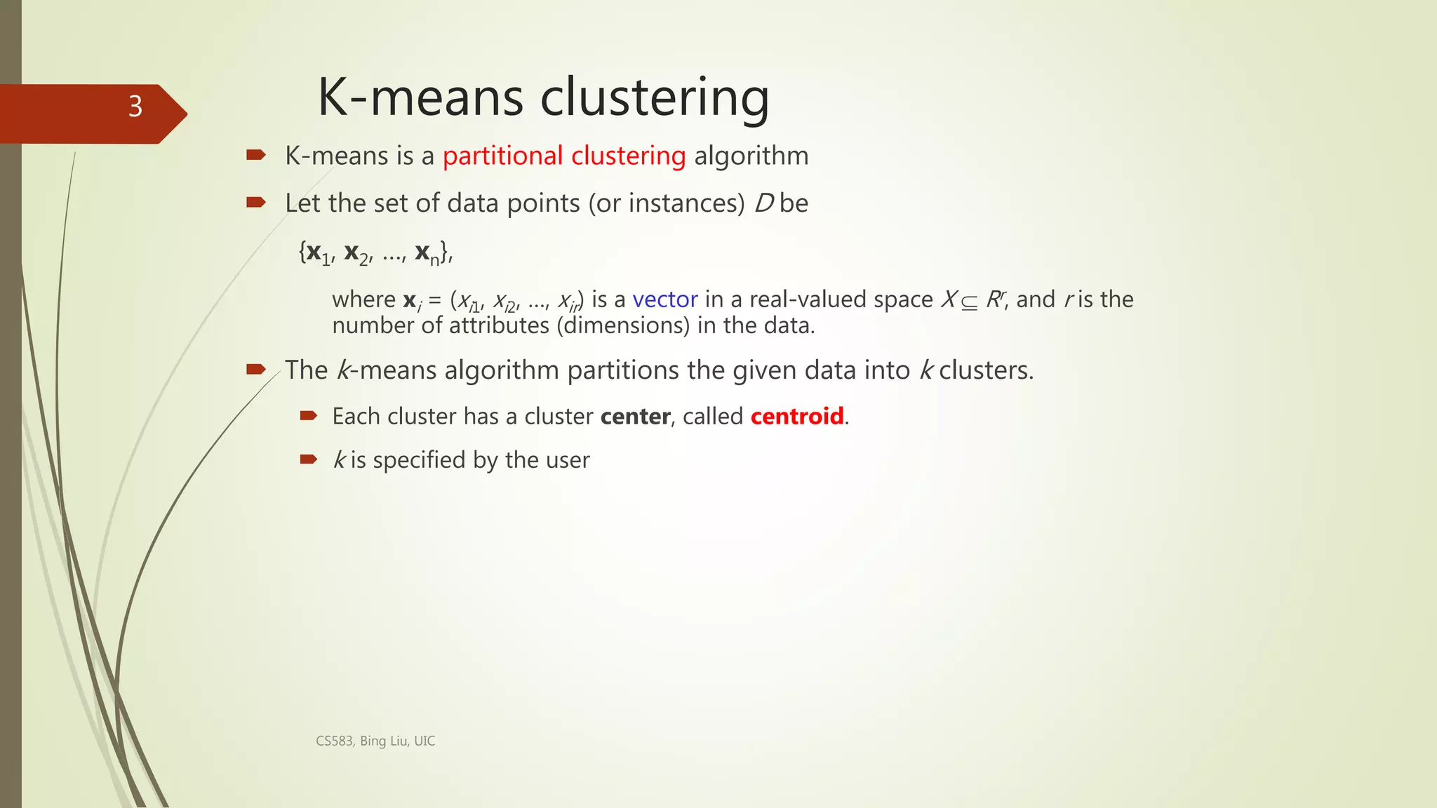
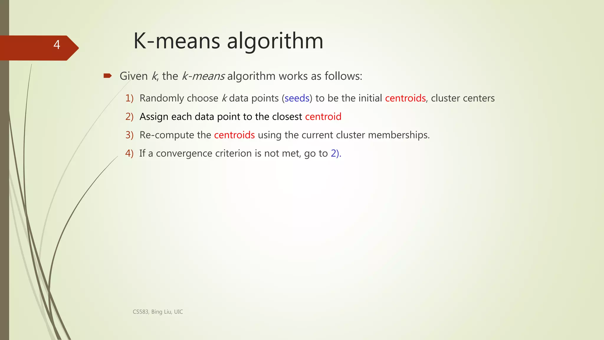
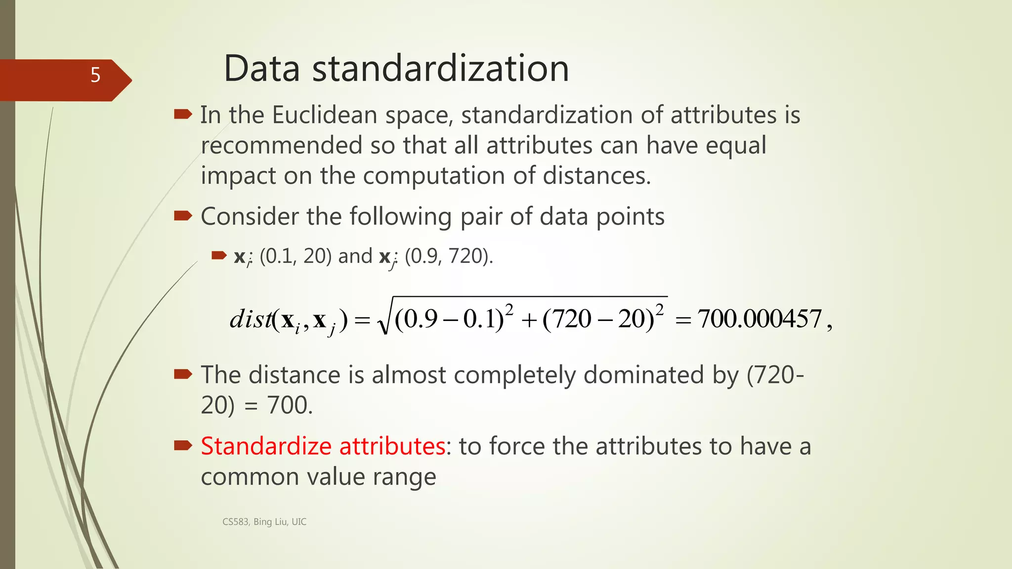
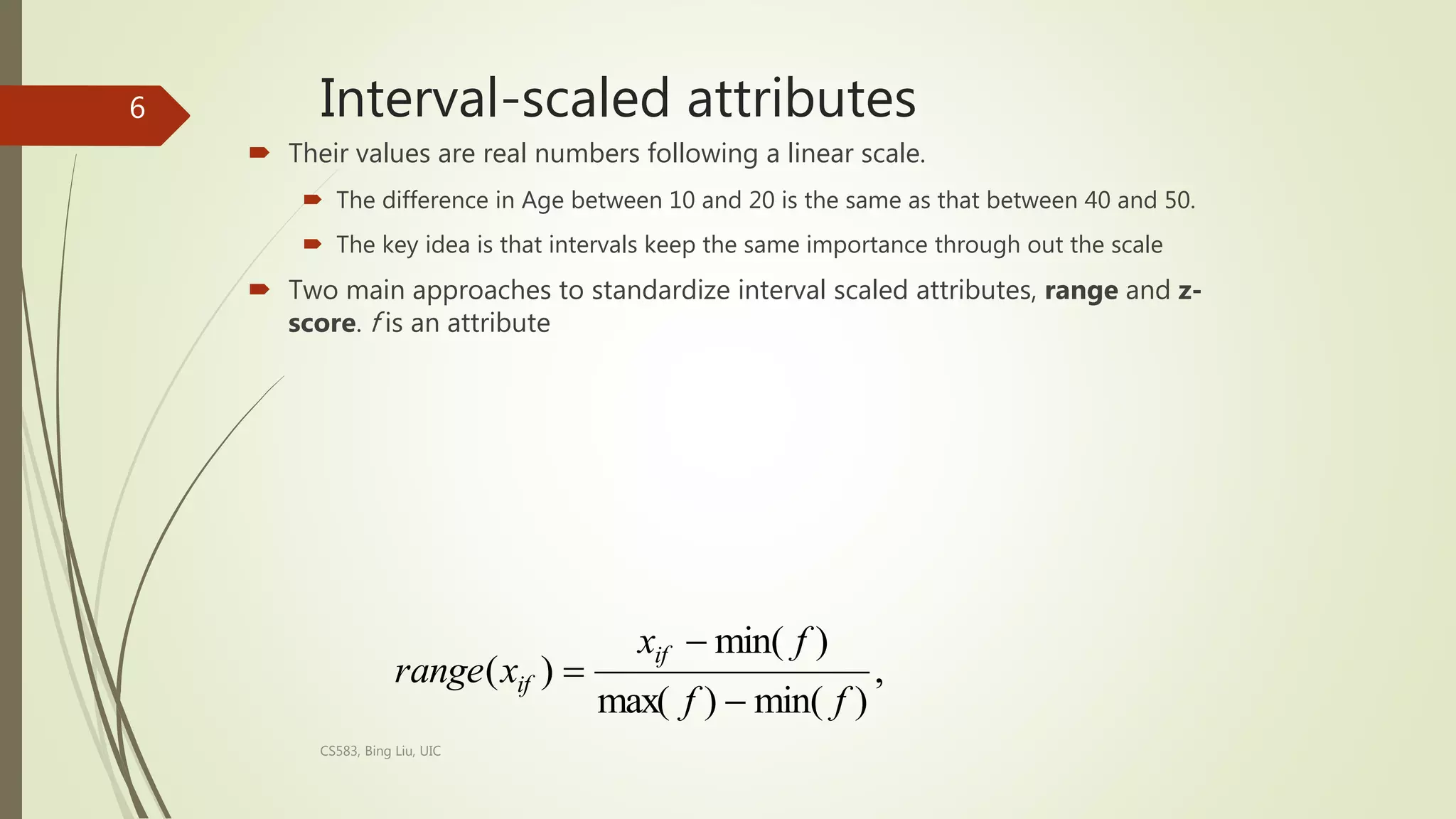
Presentation on unsupervised learning

Presentation on
Unsupervised Learning
ANKUSH PAL
MBA – 172
12019001001172

Supervised learning vs. unsupervised
learning
 Supervised learning: discover patterns in the data that relate data attributes
with a target (class) attribute.
 These patterns are then utilized to predict the values of the target attribute in
future data instances.
 Unsupervised learning: The data have no target attribute.
 We want to explore the data to find some intrinsic structures in them.
CS583, Bing Liu, UIC
2

K-means clustering
 K-means is a partitional clustering algorithm
 Let the set of data points (or instances) D be
{x1, x2, …, xn},
where xi = (xi1, xi2, …, xir) is a vector in a real-valued space X  Rr, and r is the
number of attributes (dimensions) in the data.
 The k-means algorithm partitions the given data into k clusters.
 Each cluster has a cluster center, called centroid.
 k is specified by the user
3

K-means algorithm
 Given k, the k-means algorithm works as follows:
1) Randomly choose k data points (seeds) to be the initial centroids, cluster centers
2) Assign each data point to the closest centroid
3) Re-compute the centroids using the current cluster memberships.
4) If a convergence criterion is not met, go to 2).
4

Data standardization
 In the Euclidean space, standardization of attributes is
recommended so that all attributes can have equal
impact on the computation of distances.
 Consider the following pair of data points
 xi: (0.1, 20) and xj: (0.9, 720).
 The distance is almost completely dominated by (720-
20) = 700.
 Standardize attributes: to force the attributes to have a
common value range
5
,
700.000457
)
20
720
(
)
1
.
0
9
.
0
(
)
,
( 2
2





j
i
dist x
x

Interval-scaled attributes
 Their values are real numbers following a linear scale.
 The difference in Age between 10 and 20 is the same as that between 40 and 50.
 The key idea is that intervals keep the same importance through out the scale
 Two main approaches to standardize interval scaled attributes, range and z-
score. f is an attribute
6
,
)
min(
)
max(
)
min(
)
(
f
f
f
x
x
range
if
if




Cluster Evaluation: hard problem
 The quality of a clustering is very hard to evaluate because
 We do not know the correct clusters
 Some methods are used:
 User inspection
 Study centroids, and spreads
 Rules from a decision tree.
 For text documents, one can read some documents in clusters.
7

Cluster evaluation: ground truth
 We use some labeled data (for classification)
 Assumption: Each class is a cluster.
 After clustering, a confusion matrix is constructed. From the matrix, we
compute various measurements, entropy, purity, precision, recall and F-score.
 Let the classes in the data D be C = (c1, c2, …, ck). The clustering method produces k
clusters, which divides D into k disjoint subsets, D1, D2, …, Dk.
8

Supervised learning for unsupervised
learning
 Decision tree algorithm is not directly applicable.
 it needs at least two classes of data.
 A clustering data set has no class label for each data point.
 The problem can be dealt with by a simple idea.
 Regard each point in the data set to have a class label Y.
 Assume that the data space is uniformly distributed with another
type of points, called non-existing points. We give them the
class, N.
 With the N points added, the problem of partitioning the
data space into data and empty regions becomes a
supervised classification problem.
9

An example
10
A decision tree method is used for partitioning in (B).

Building the Tree
 The main computation in decision tree building is to
evaluate entropy (for information gain):
 Can it be evaluated without adding N points? Yes.
 Pr(cj) is the probability of class cj in data set D, and |C| is
the number of classes, Y and N (2 classes).
 To compute Pr(cj), we only need the number of Y (data) points
and the number of N (non-existing) points.
 We already have Y (or data) points, and we can compute the
number of N points on the fly. Simple: as we assume that the N
points are uniformly distributed in the space.
11
)
Pr(
log
)
Pr(
)
(
|
|
1
2 j
C
j
j c
c
D
entropy 




An example
 The space has 25 data (Y) points and 25 N points.
Assume the system is evaluating a possible cut S.
 # N points on the left of S is 25 * 4/10 = 10. The number of Y
points is 3.
 Likewise, # N points on the right of S is 15 (= 25 - 10).The
number of Y points is 22.
 With these numbers, entropy can be computed.
CS583, Bing Liu, UIC 12

Presentation on unsupervised learning

More Related Content

What's hot

Similar to Presentation on unsupervised learning

More from ANKUSH PAL

Recently uploaded

Presentation on unsupervised learning