Download to read offline


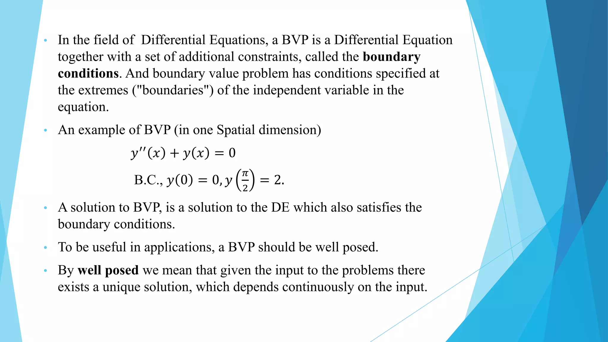
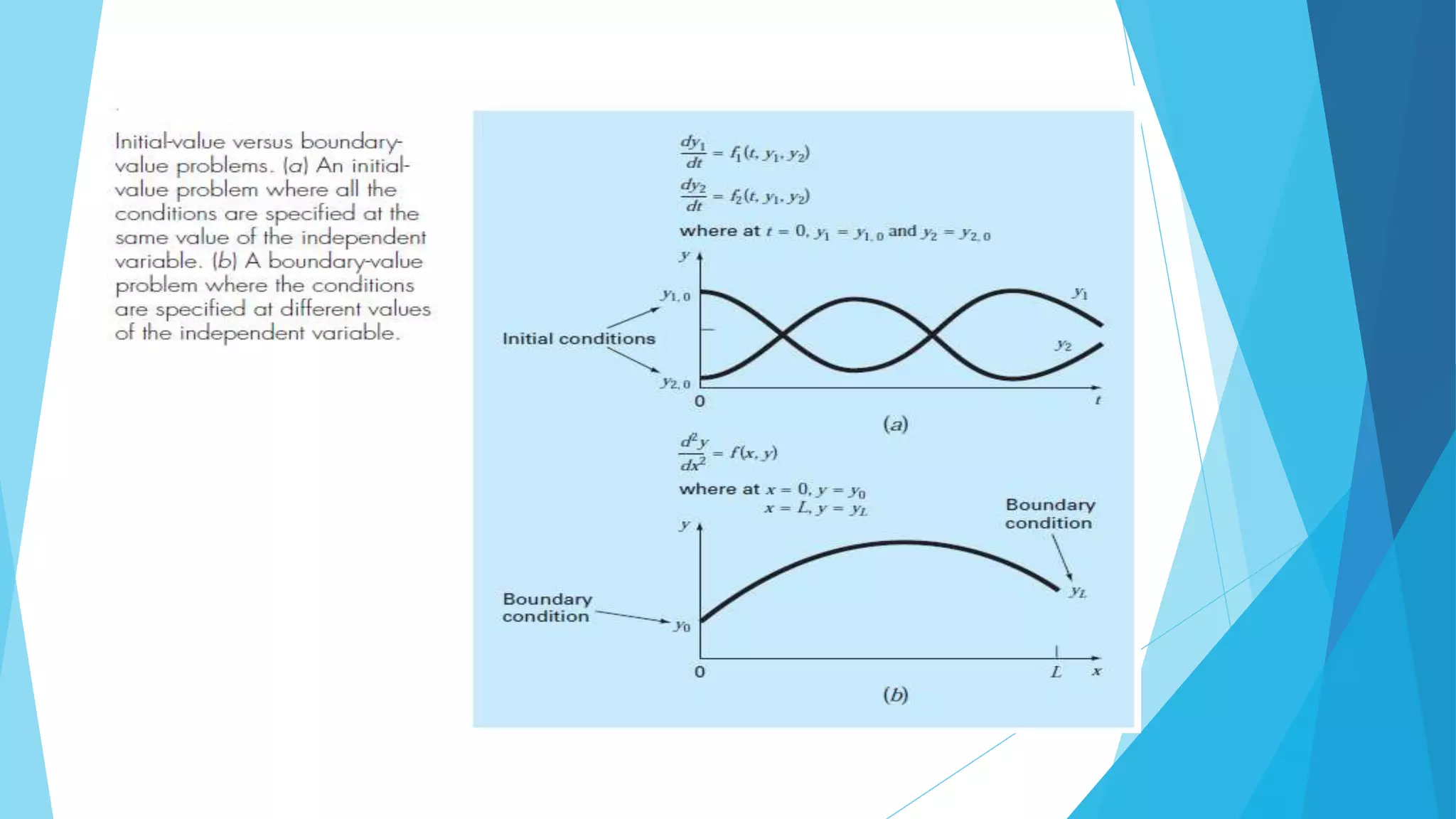

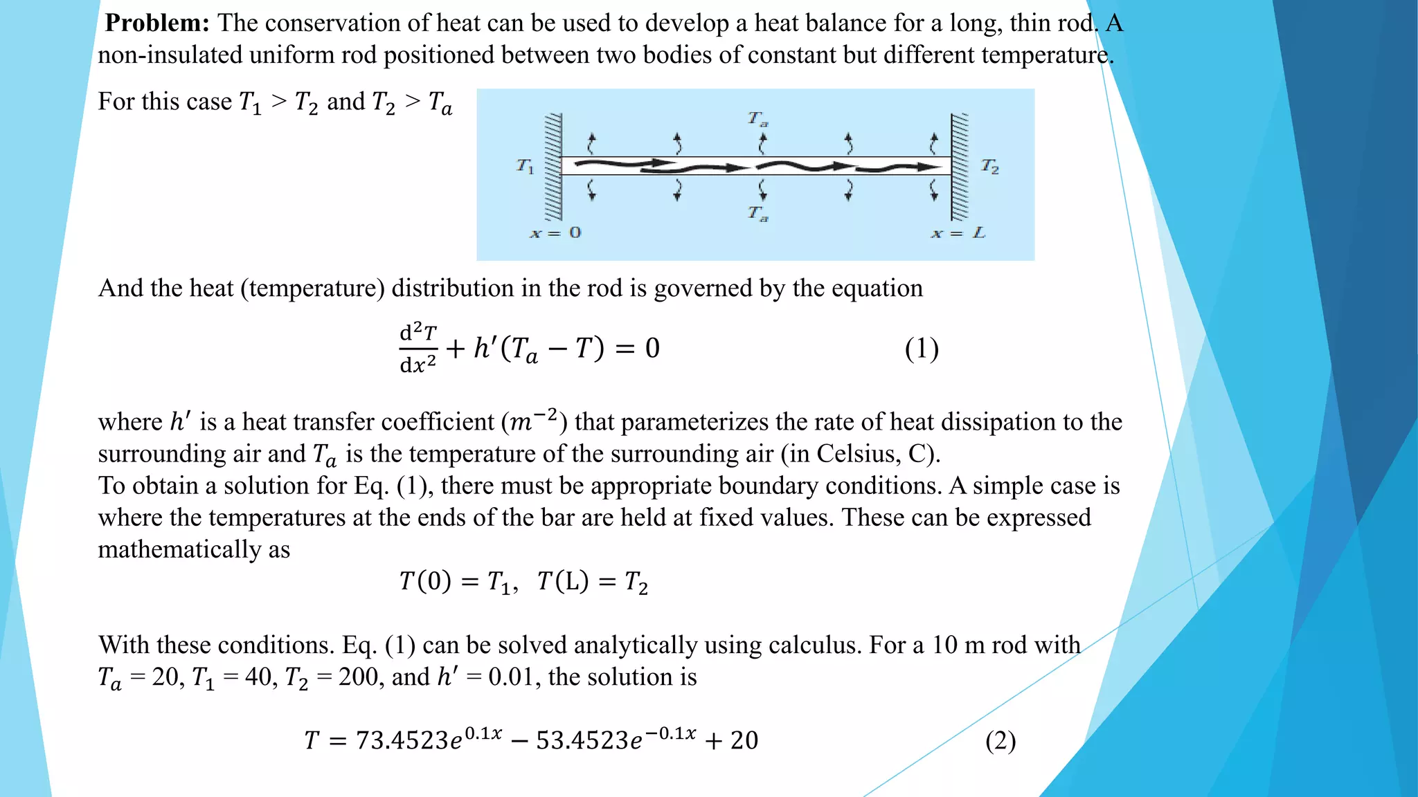


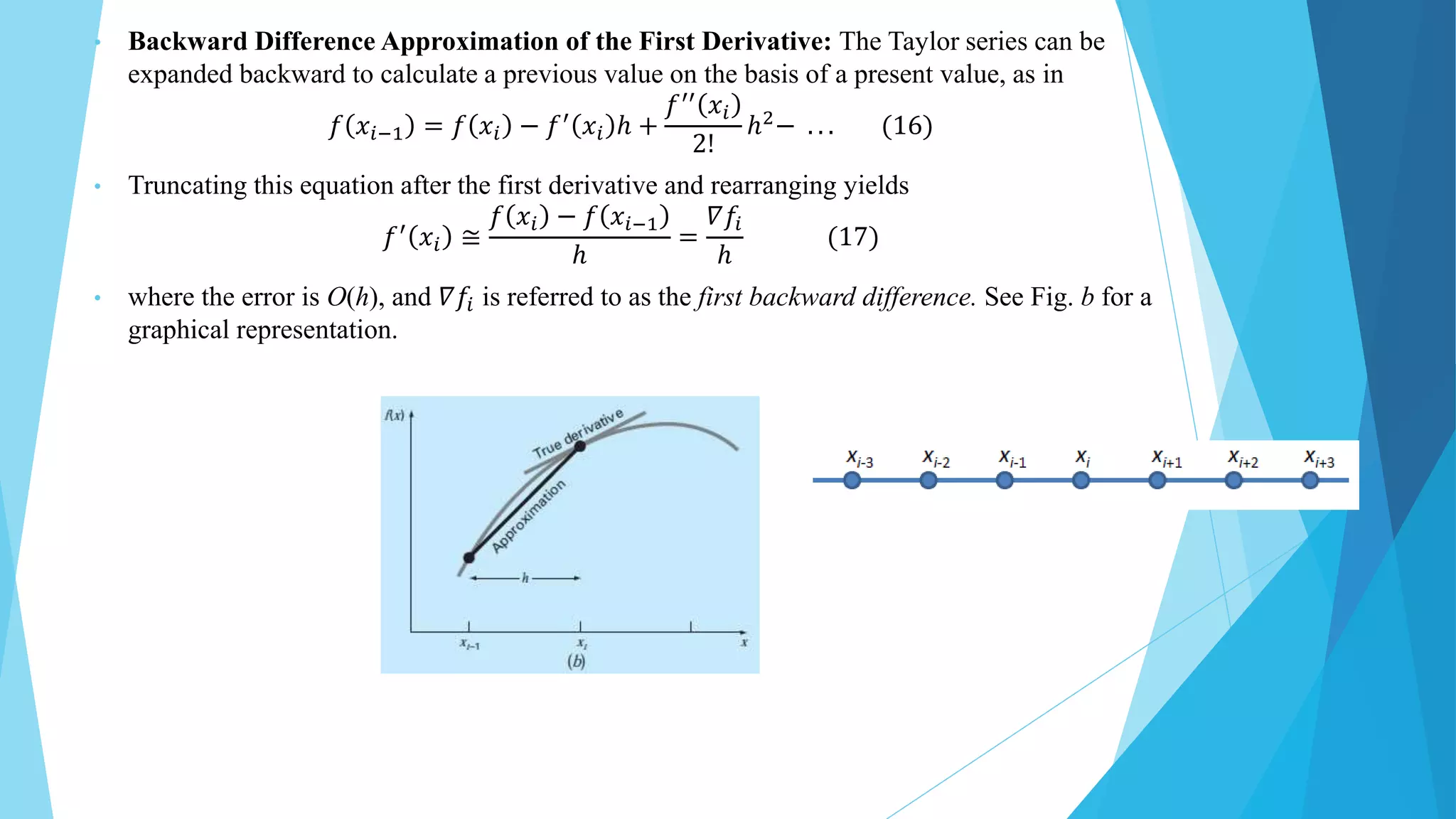
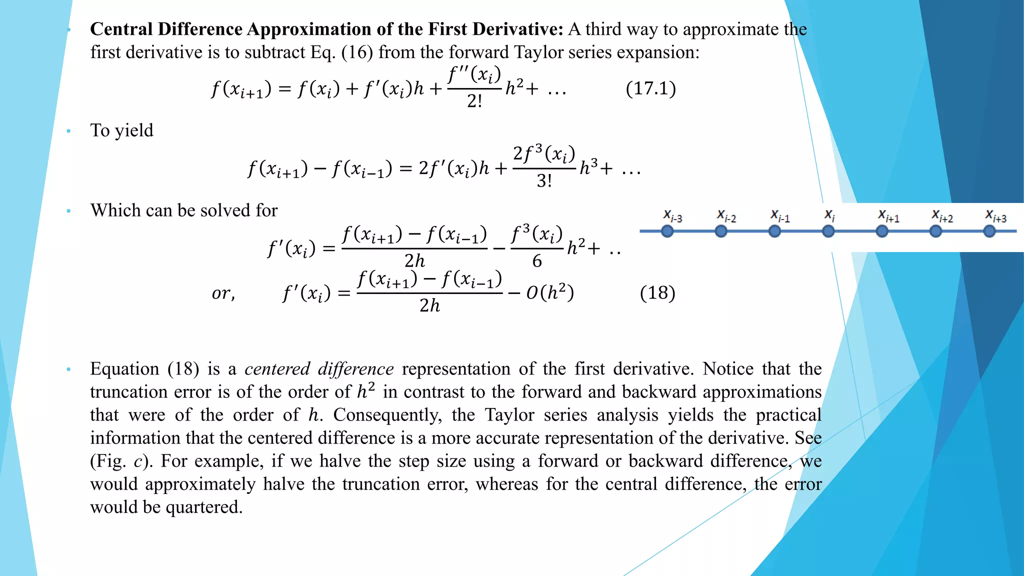
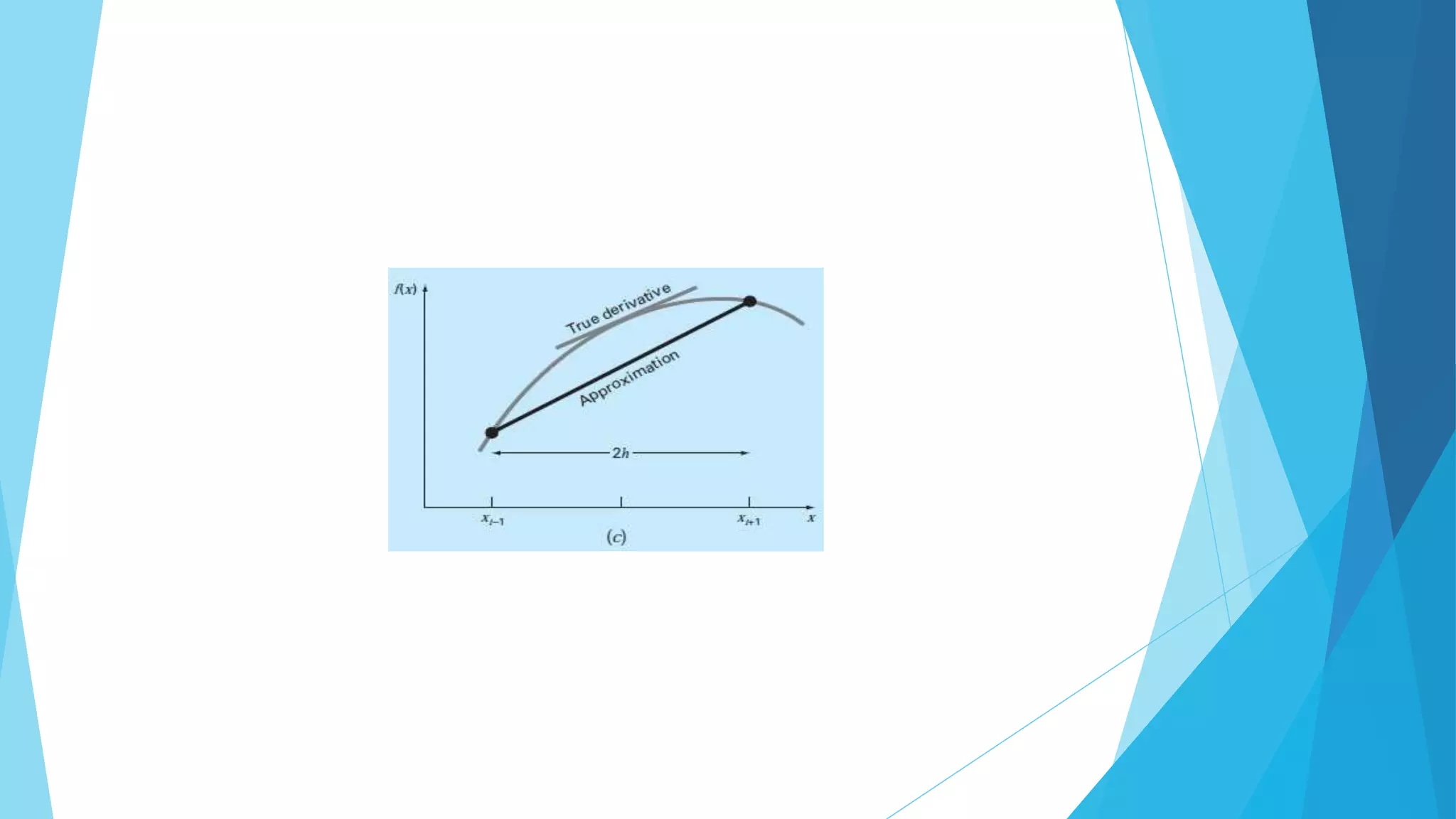
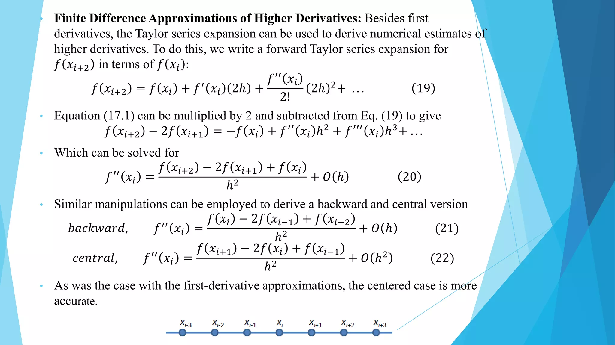
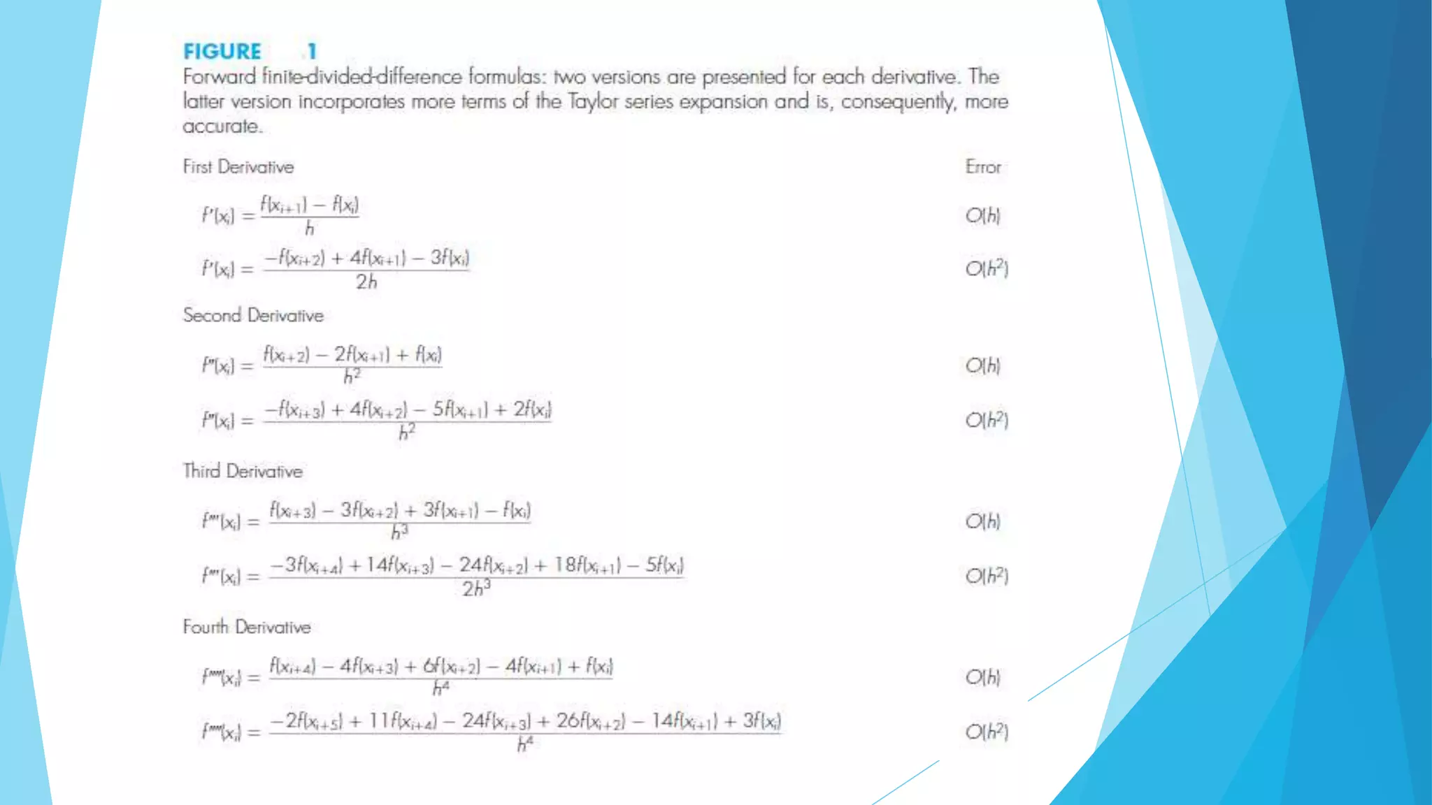
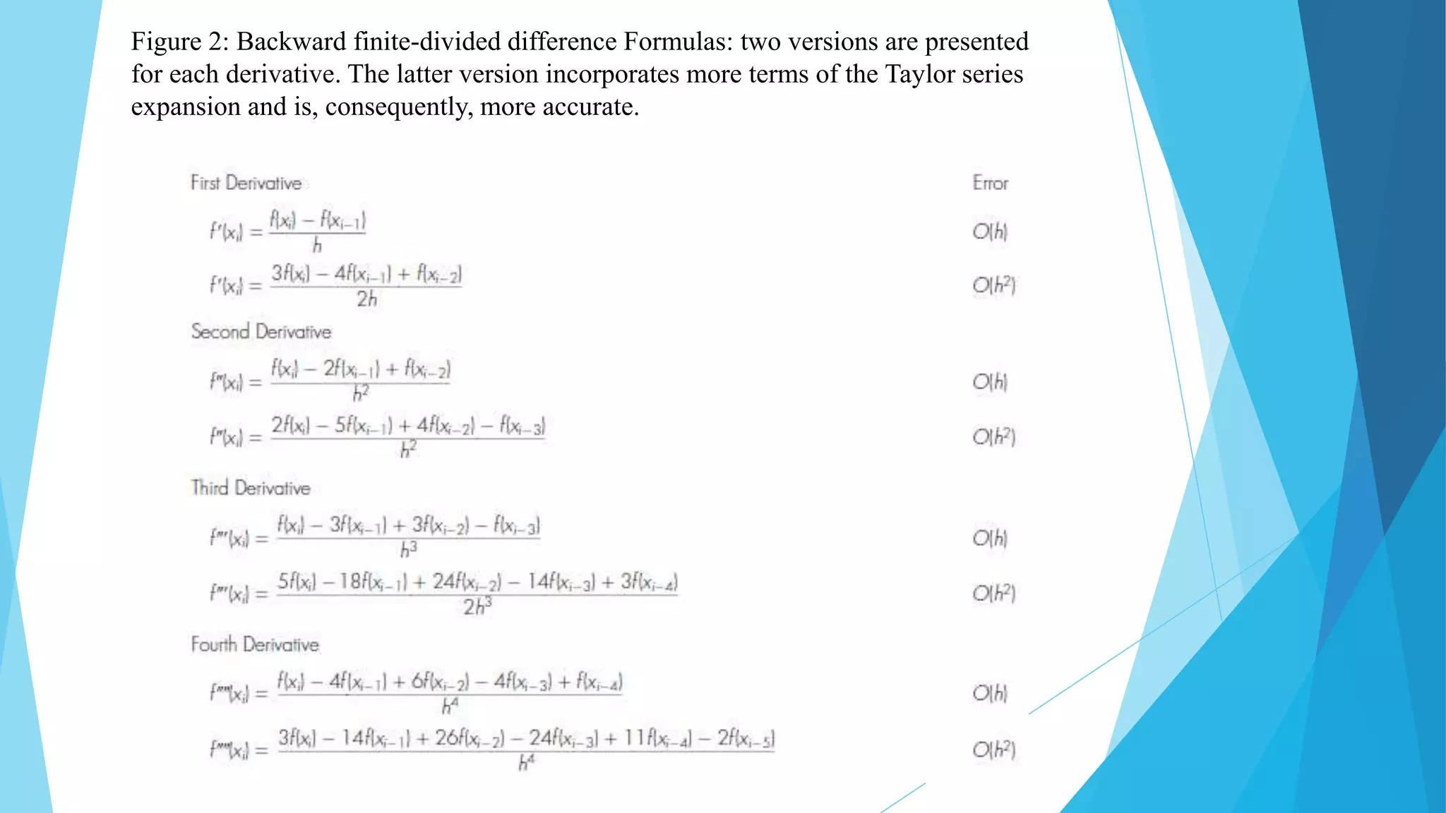
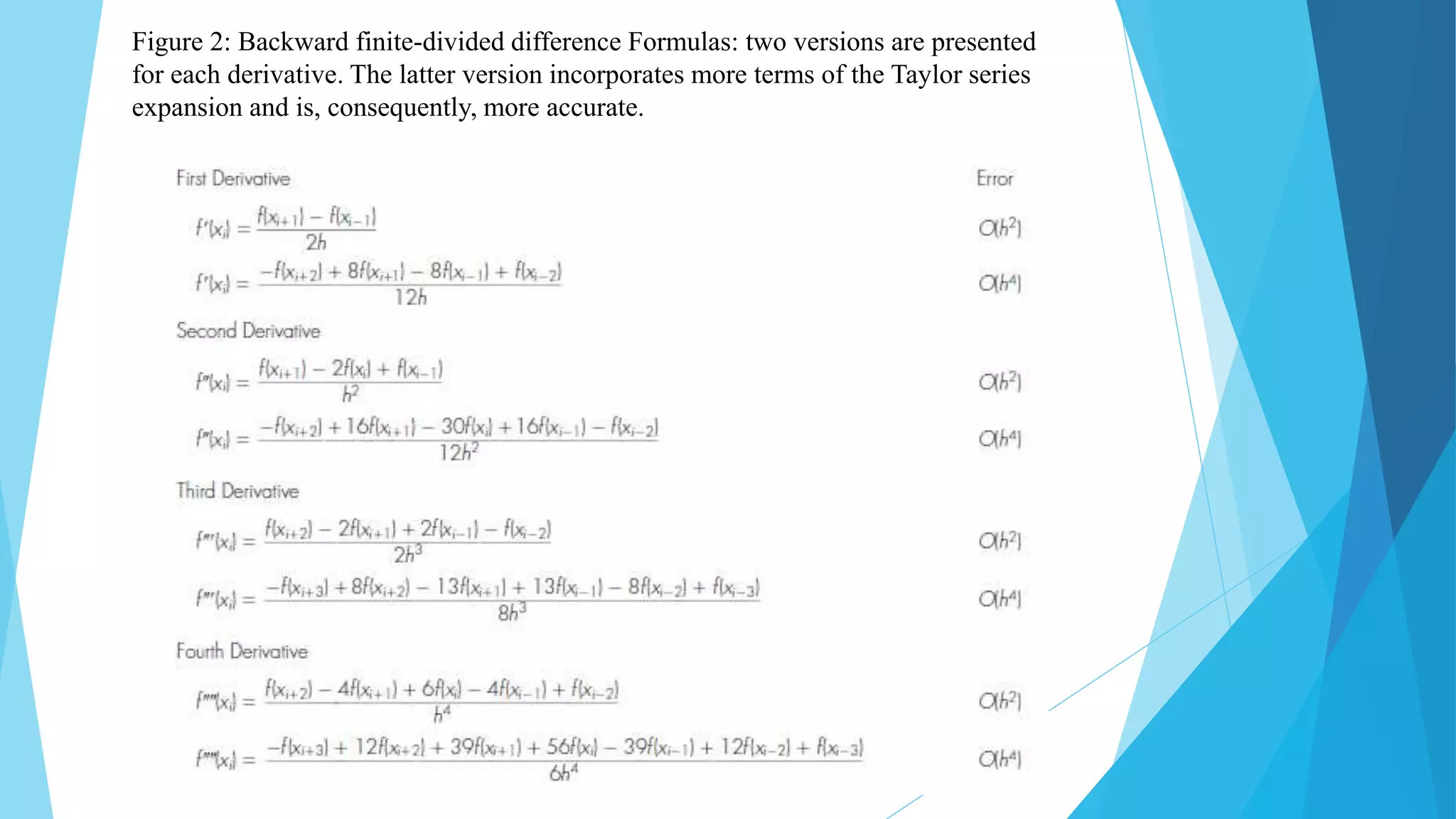

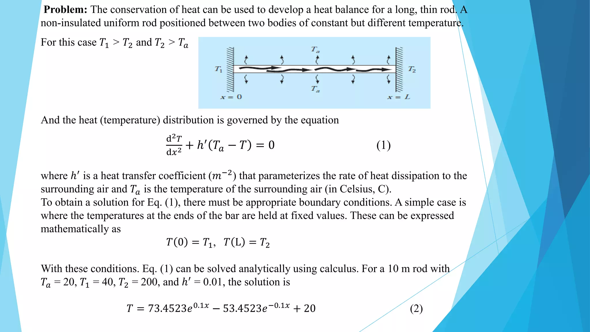
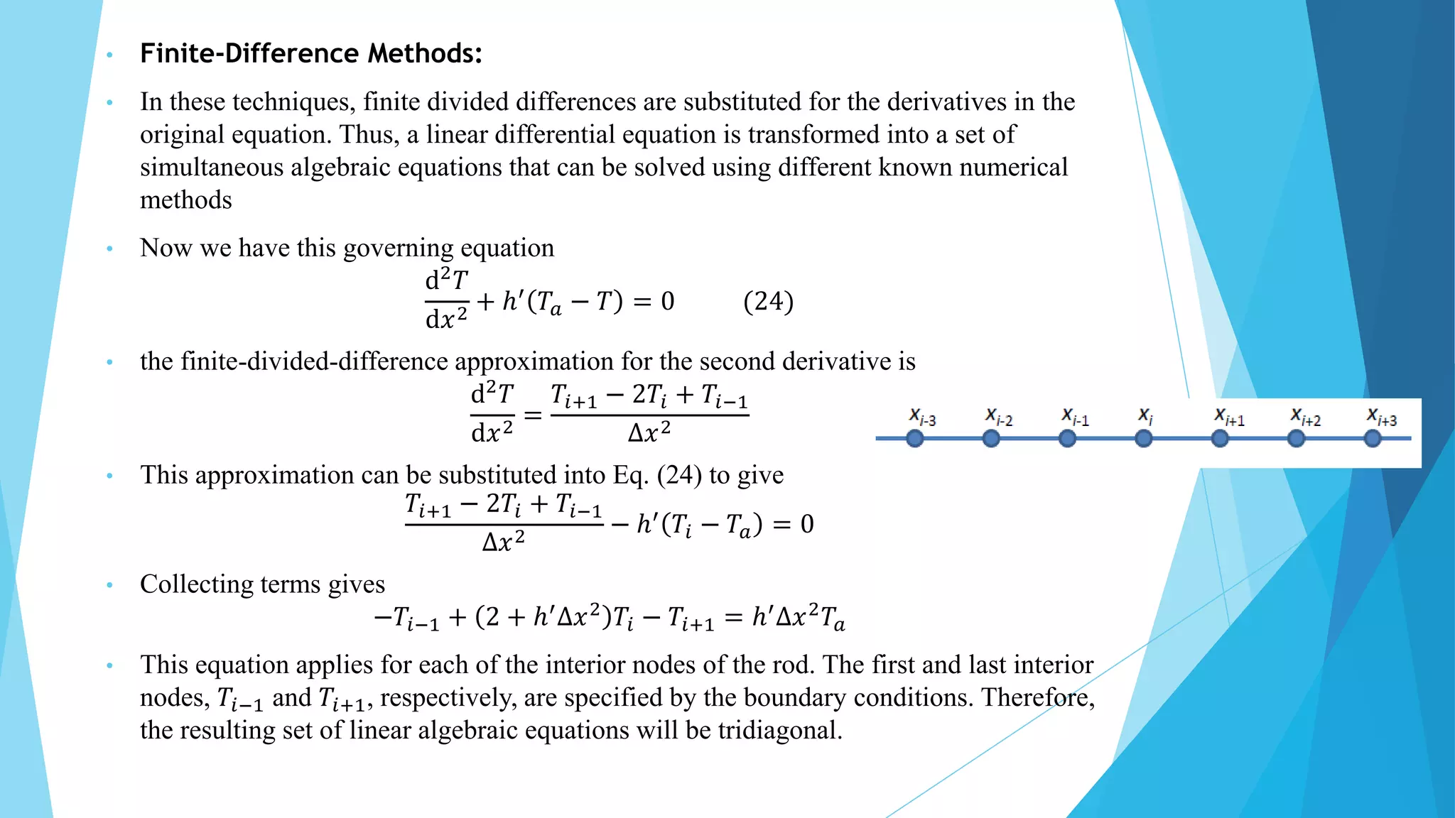
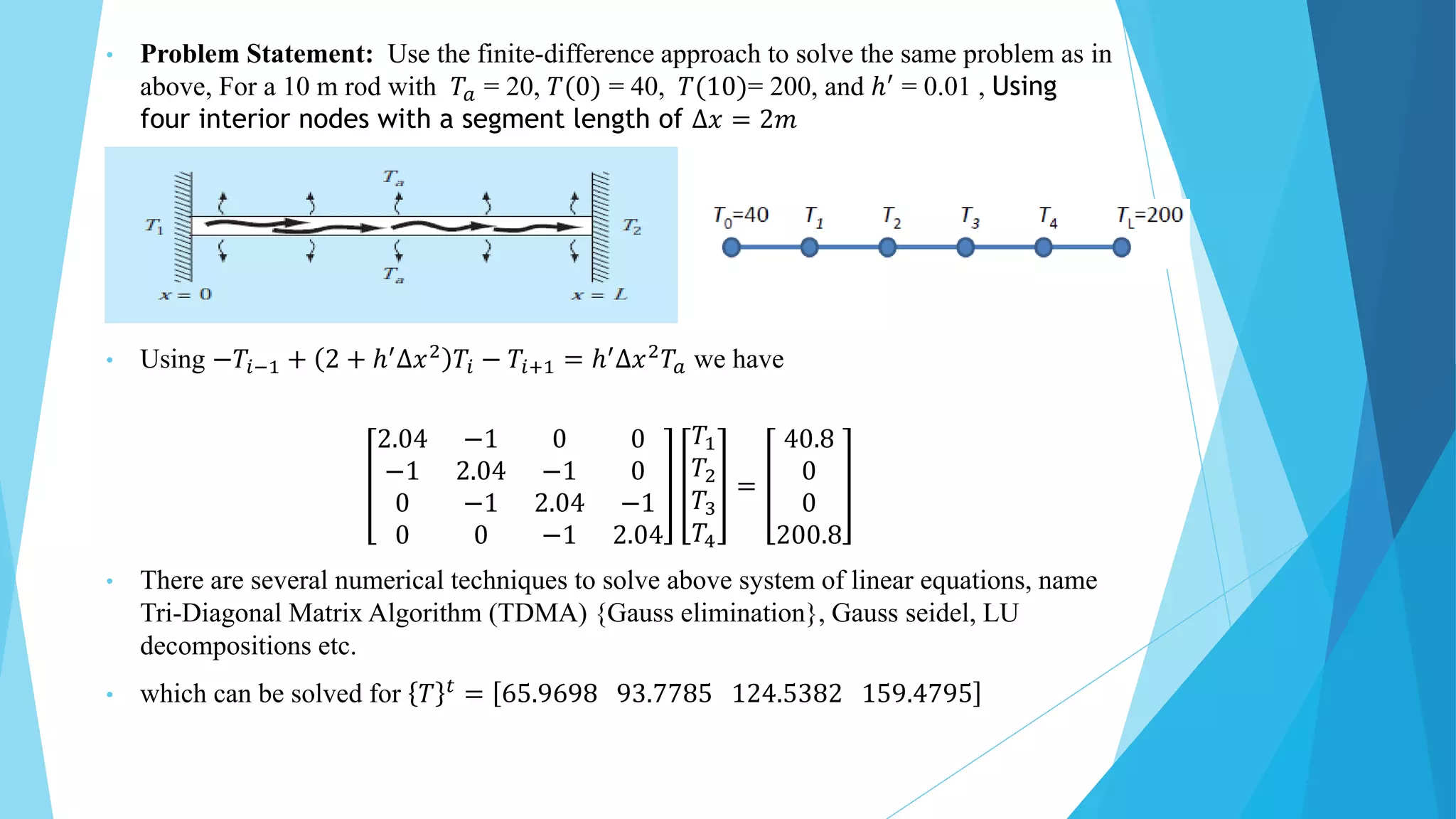
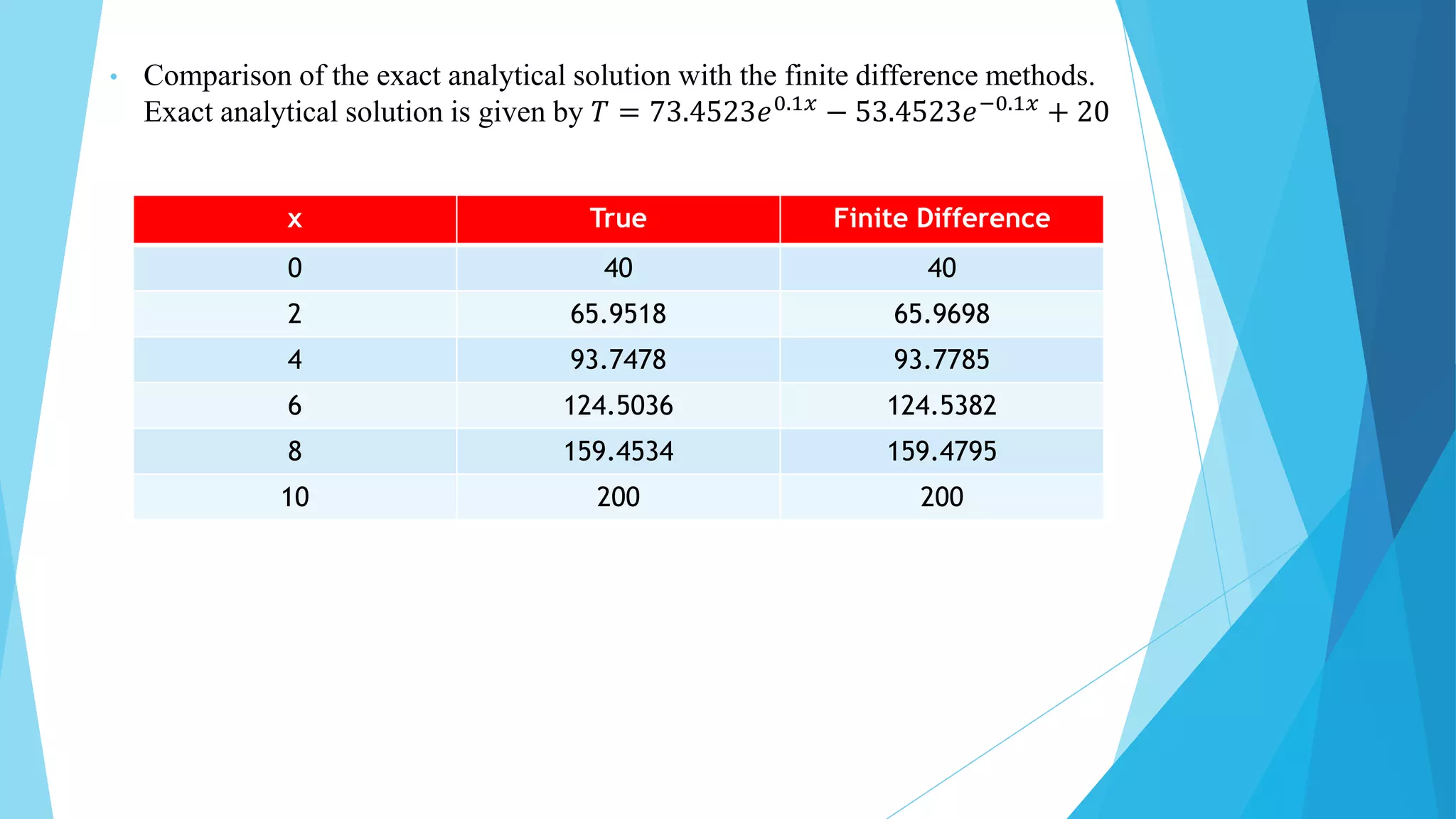
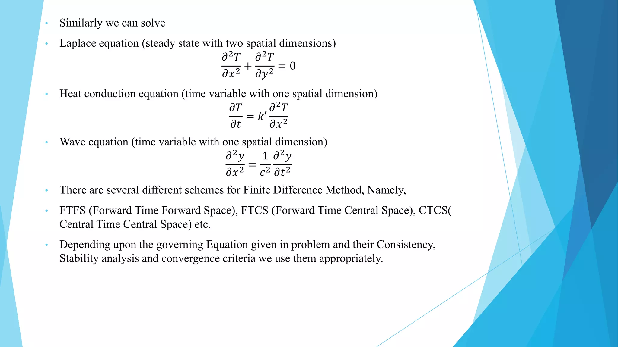


The document discusses the application of numerical analysis, specifically focusing on boundary value problems (BVP) and how numerical methods such as the finite difference method (FDM) can be used to approximate solutions when analytical solutions are difficult to obtain. It includes examples of BVP in the context of heat distribution in a rod and illustrates the finite divided difference technique for numerical differentiation and its connection to the Taylor series expansion. Furthermore, it presents the comparison between exact solutions and those obtained through finite difference methods, showcasing the importance of numerical approaches in solving differential equations.