Downloaded 342 times

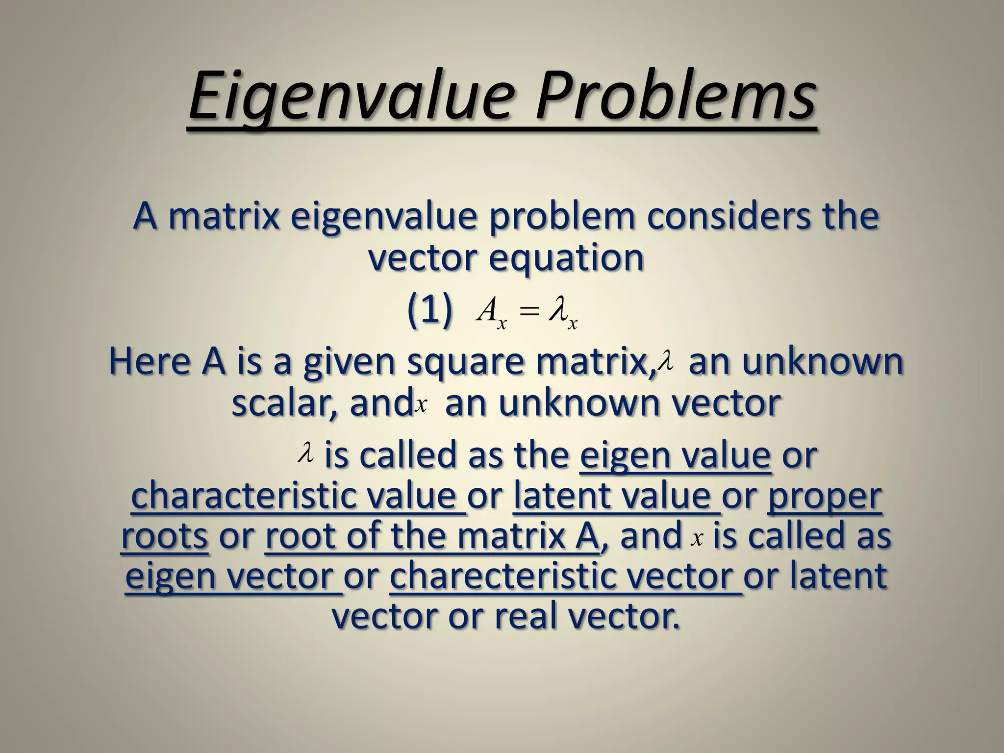
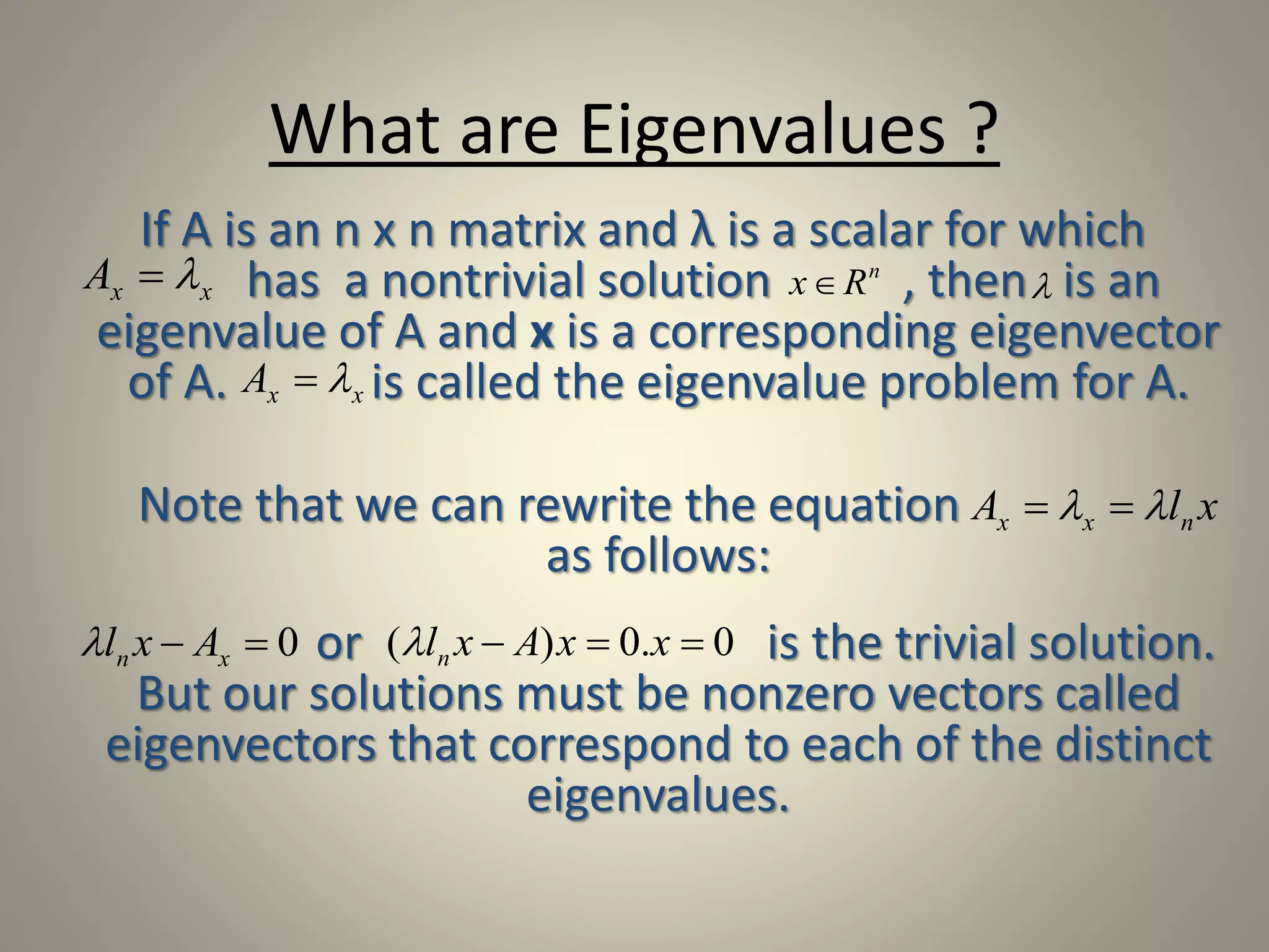
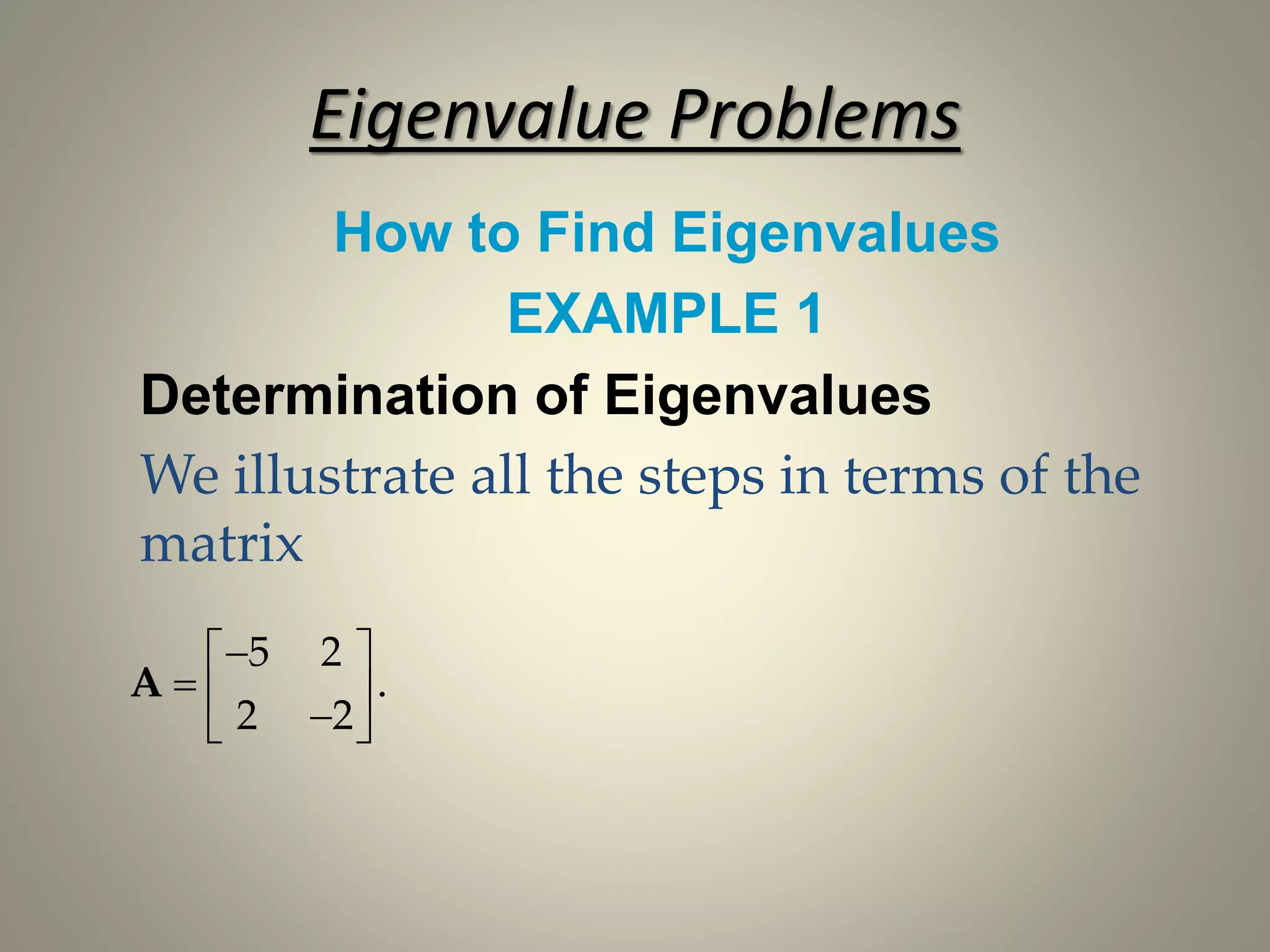
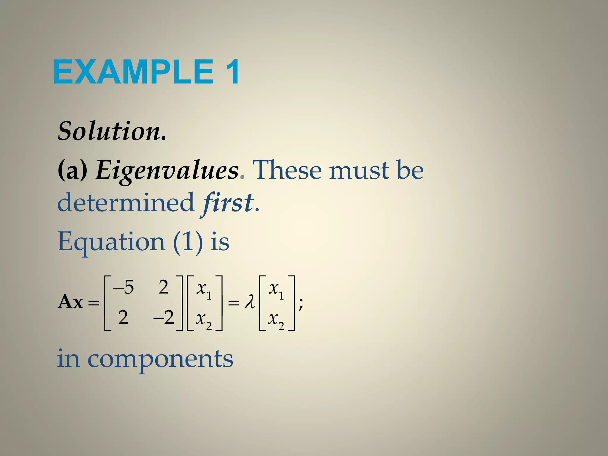
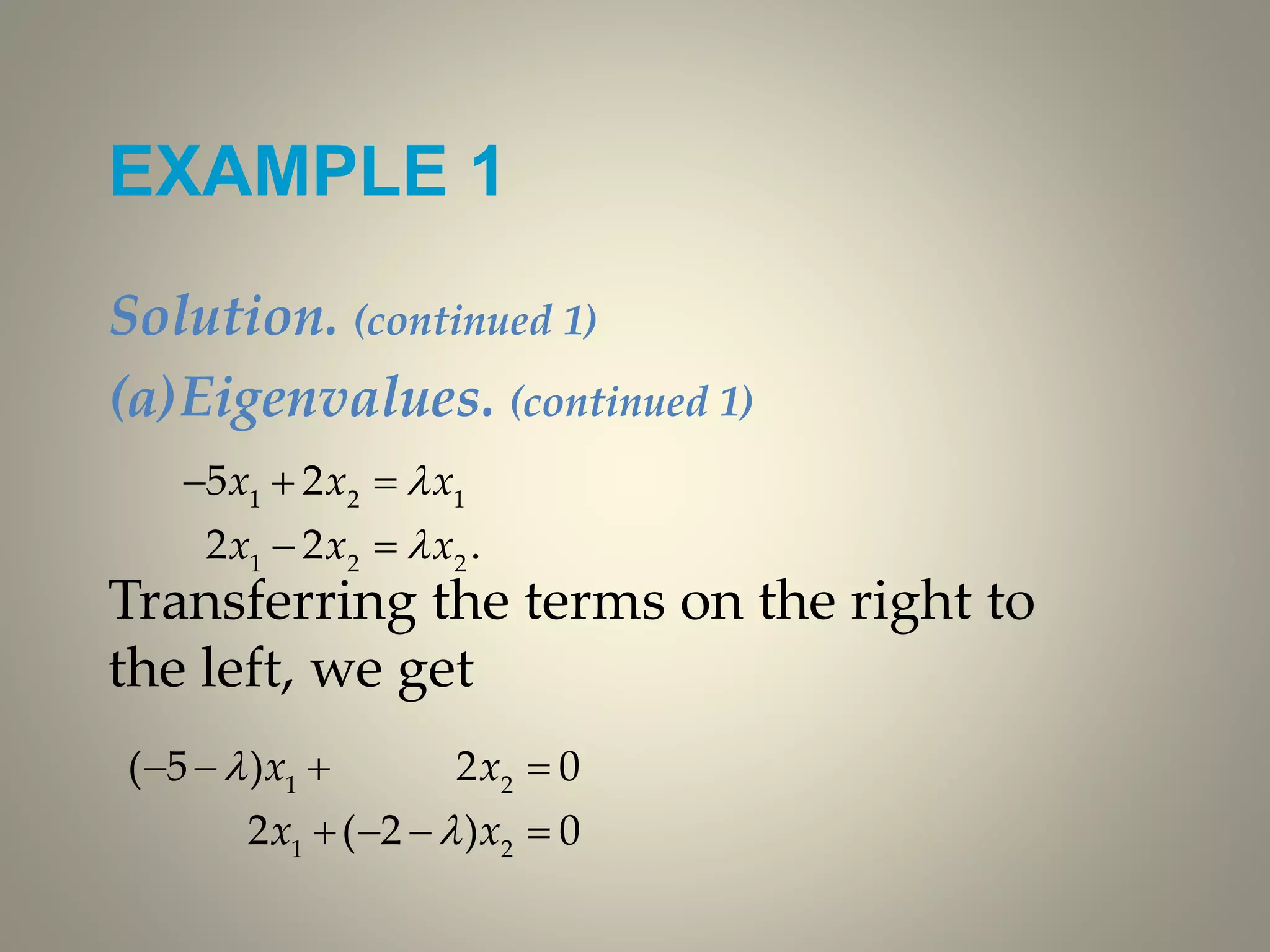

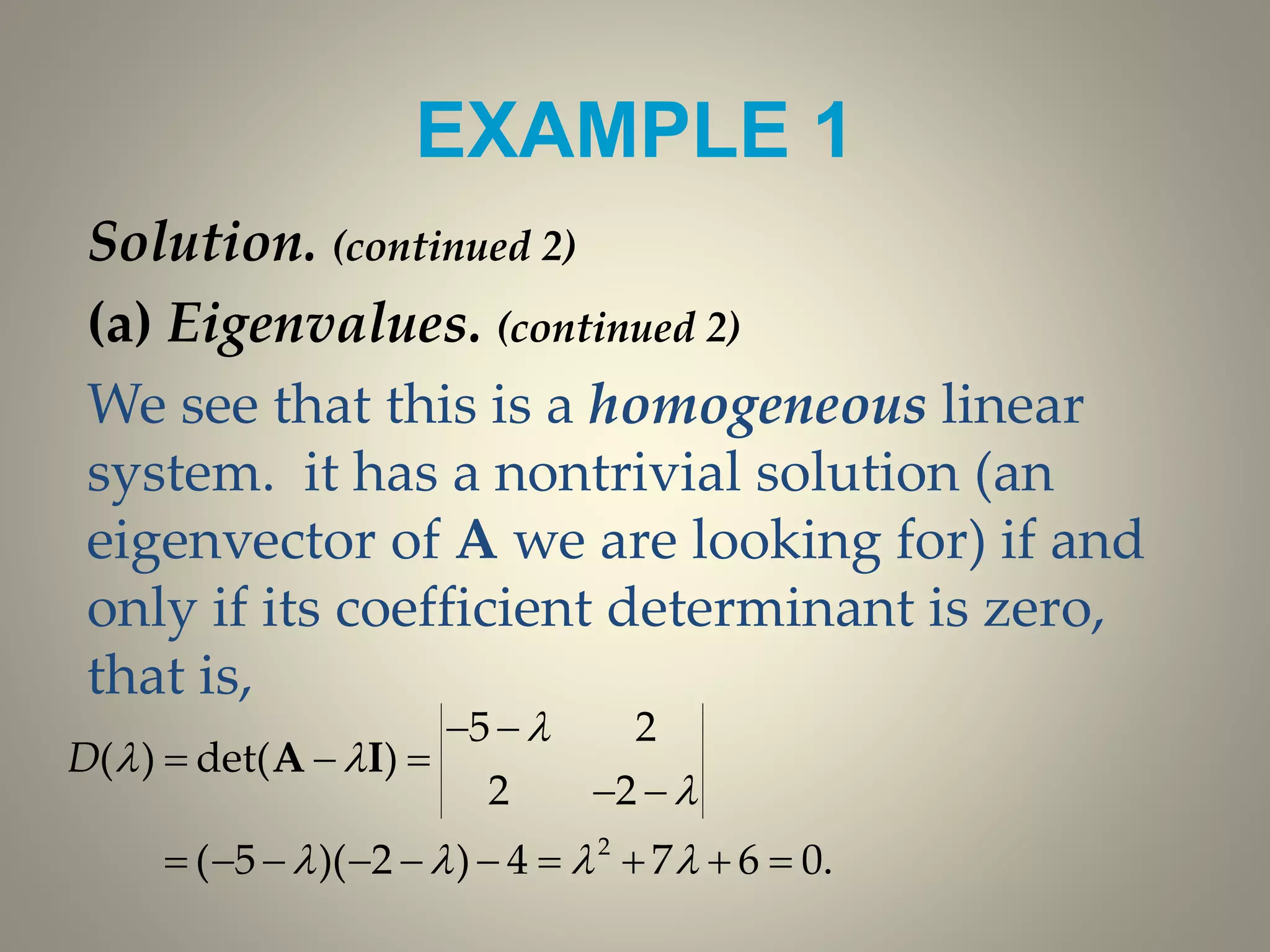
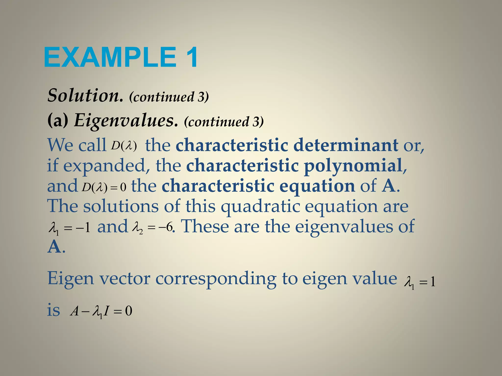

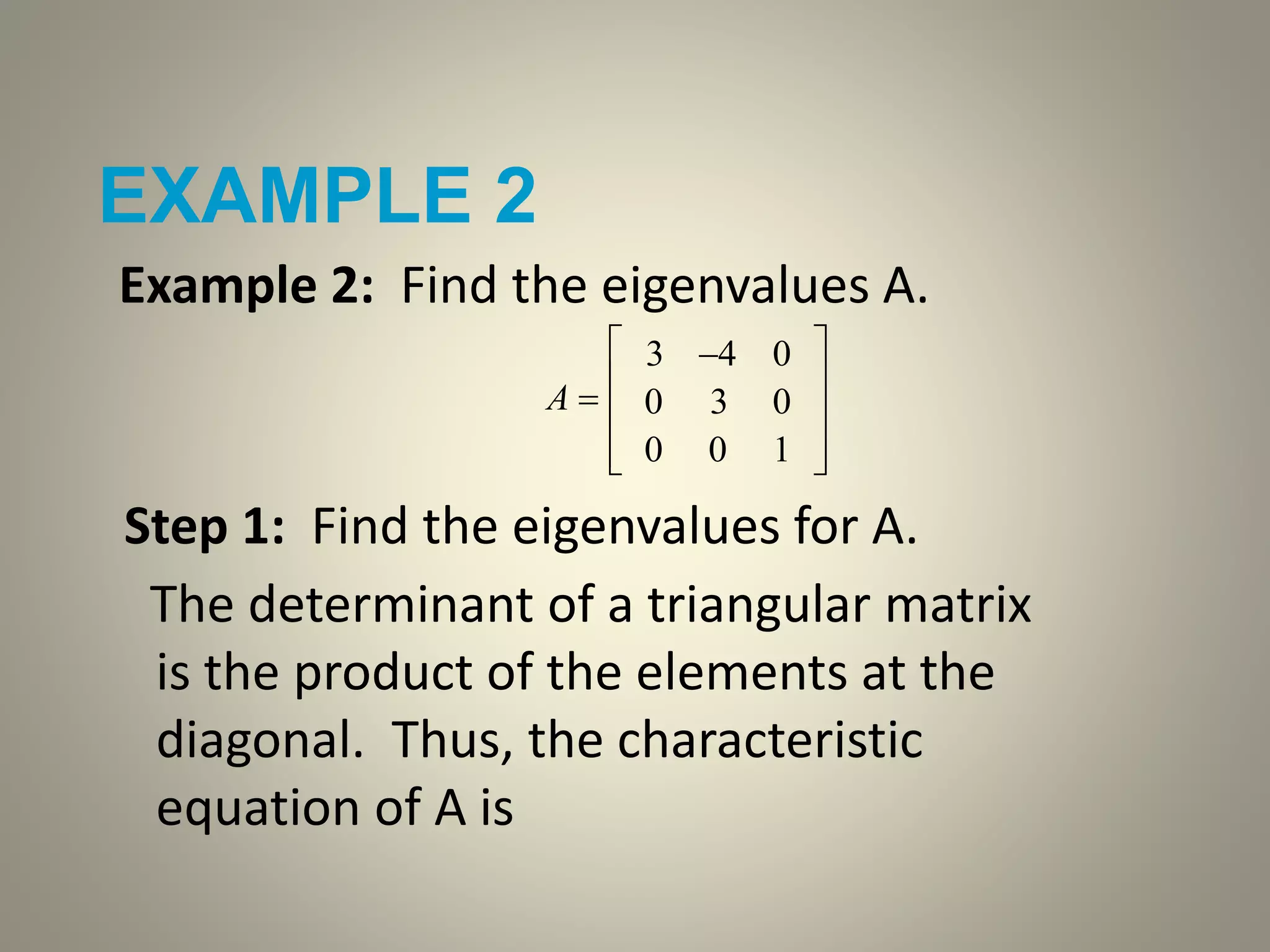
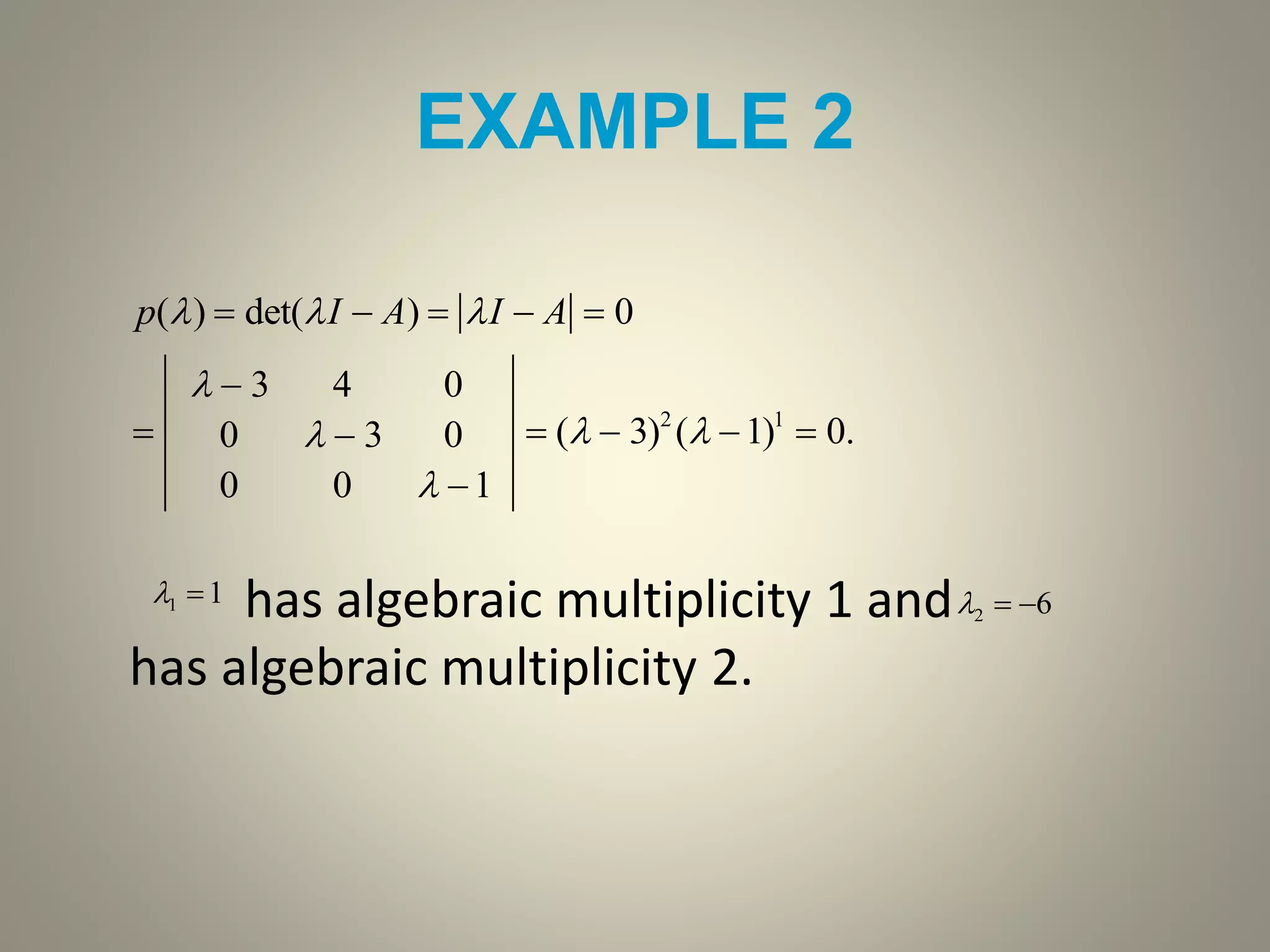
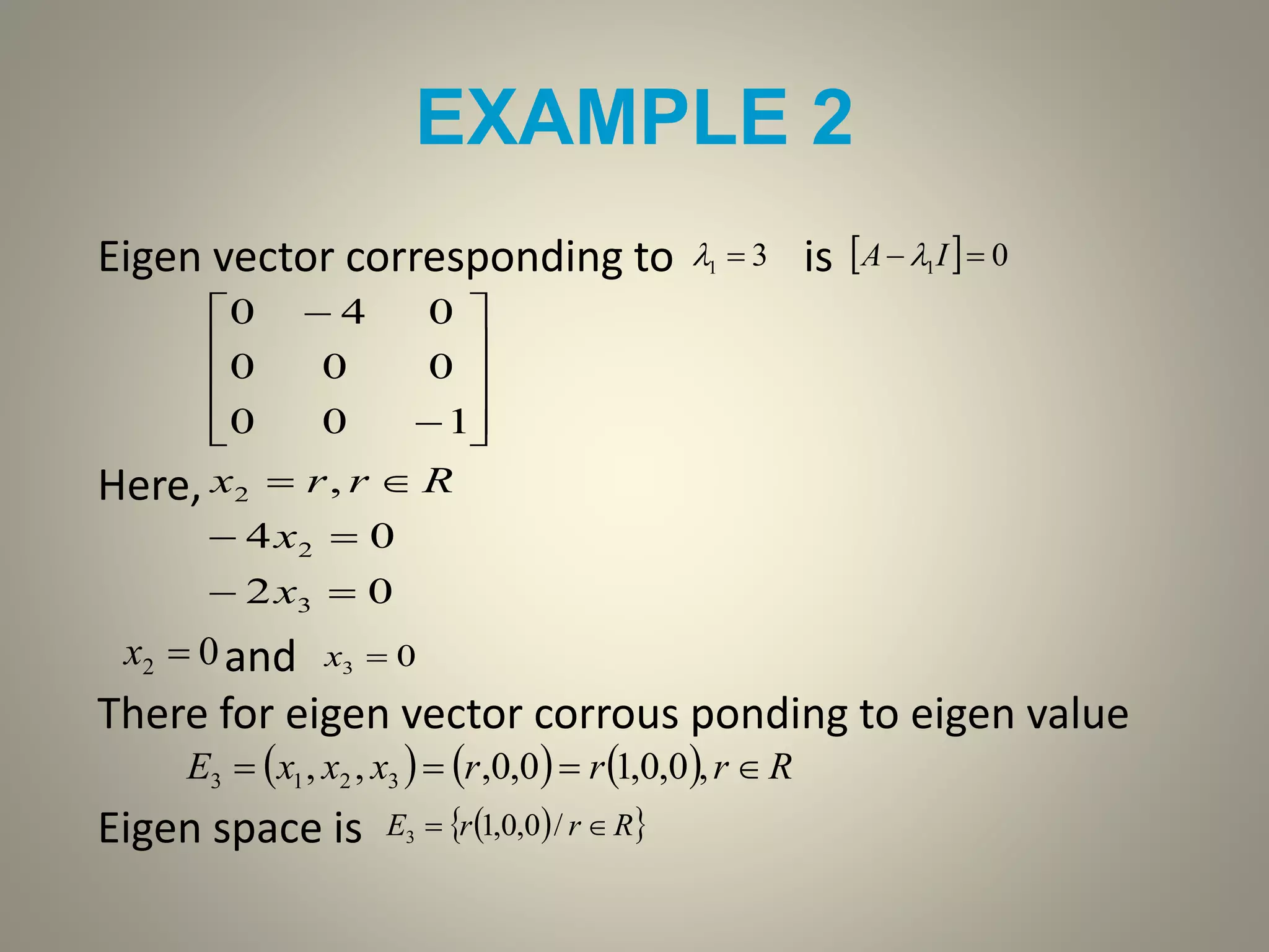
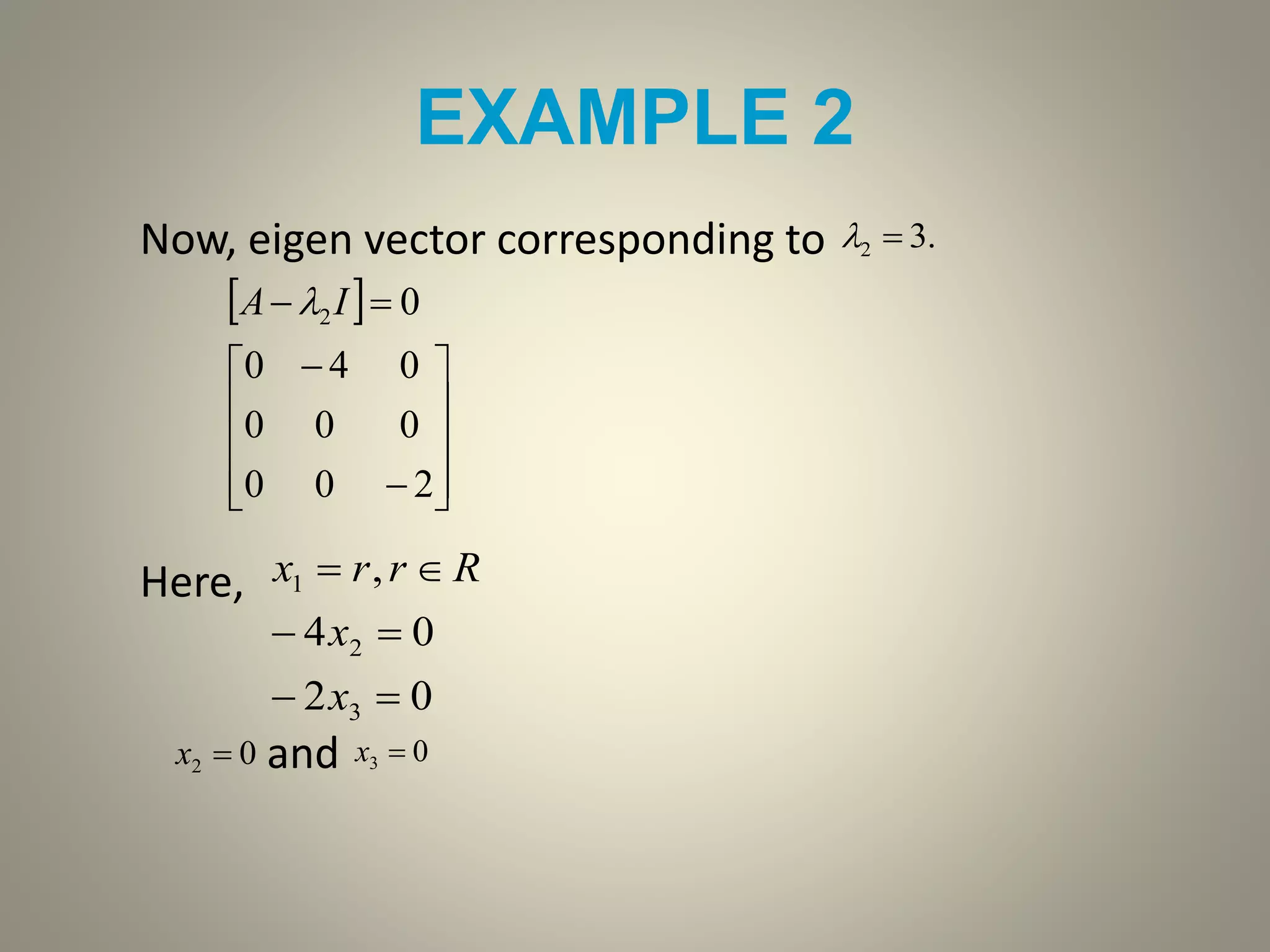
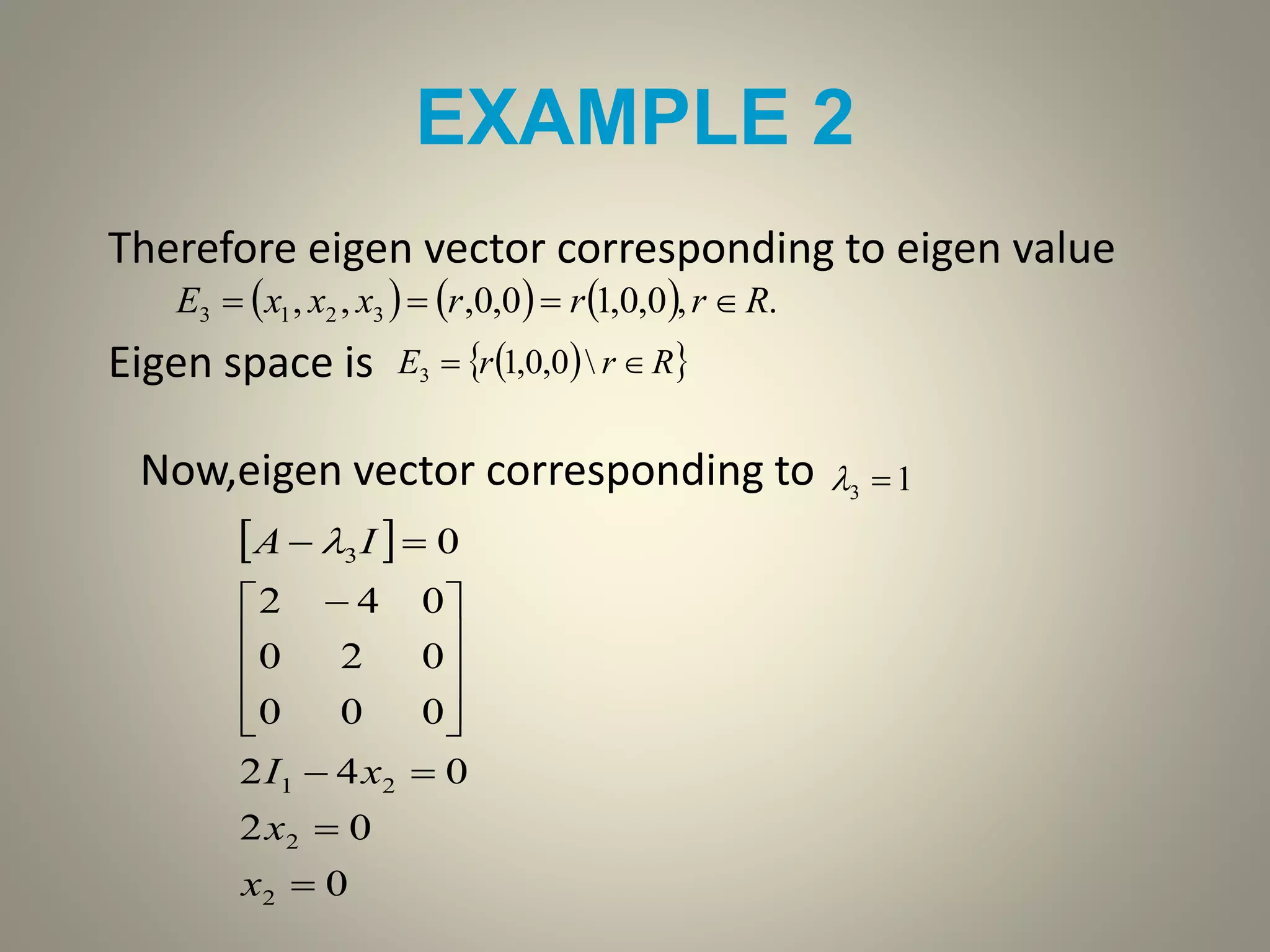
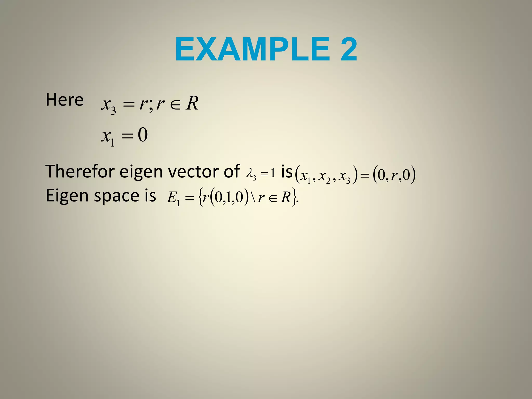


The document provides examples to illustrate how to find the eigenvalues and eigenvectors of a matrix. 1) For a 2x2 matrix, the characteristic polynomial is computed by taking the determinant of the matrix minus the identity matrix. The roots of the characteristic polynomial are the eigenvalues. The corresponding eigenvectors are found by solving the original eigenvalue equation. 2) For a triangular matrix, the eigenvalues are the diagonal elements. The eigenvectors are found by setting rows corresponding to non-diagonal elements to zero. 3) The document provides a numerical example to demonstrate finding the eigenvalues (3, 1, -2) and eigenvectors of a 3x3 matrix.