Download to read offline
![Draft version January 10, 2025
Typeset using L
A
TEX twocolumn style in AASTeX631
MUSEQuBES: Unveiling Cosmic Web Filaments at z ≈ 3.6 through Dual Absorption and Emission
Line Analysis
Eshita Banerjee ,1
Sowgat Muzahid ,1
Joop Schaye,2
Sebastiano Cantalupo,3
and Sean D. Johnson4
1IUCAA, Post Bag 04, Ganeshkhind, Pune, India, 411007
2Leiden Observatory, Leiden University, P.O. Box 9513, NL-2300 AA Leiden, the Netherlands
3Department of Physics, University of Milan Bicocca, Piazza della Scienza 3, I-20126 Milano, Italy
4Department of Astronomy, University of Michigan, 1085 S. University, Ann Arbor, MI 48109, USA
ABSTRACT
According to modern cosmological models, galaxies are embedded within cosmic filaments, which sup-
ply a continuous flow of pristine gas, fueling star formation and driving their evolution. However, due to
their low density, the direct detection of diffuse gas in cosmic filaments remains elusive. Here, we report
the discovery of an extremely metal-poor ([X/H] ≈ −3.7), low-density (log10 nH/cm−3
≈ −4, corre-
sponding to an overdensity of ≈ 5) partial Lyman limit system (pLLS) at z ≈ 3.577 along the quasar
sightline Q1317–0507, probing cosmic filaments. Additionally, two other low-metallicity ([X/H]≲ −2)
absorption systems are detected at similar redshifts, one of which is also a pLLS. VLT/MUSE obser-
vations reveal a significant overdensity of Lyα emitters (LAEs) associated with these absorbers. The
spatial distribution of the LAEs strongly suggests the presence of an underlying filamentary structure.
This is further supported by the detection of a large Lyα emitting nebula with a surface brightness of
≥ 10−19
erg cm−2
s−1
arcsec−2
, with a maximum projected linear size of ≈ 260 pkpc extending along
the LAEs. This is the first detection of giant Lyα emission tracing cosmic filaments, linked to normal
galaxies and likely powered by in-situ recombination.
Keywords: galaxies: evolution — galaxies: high-redshift — (galaxies:) quasars: absorption lines
1. INTRODUCTION
In the current cosmological framework, galaxies
emerge within the dense intersections of the cosmic
web—a large-scale network of dark matter halos and
filaments that span the universe. These structures chan-
nel gas from the intergalactic medium (IGM) into dark
matter halos, where it eventually cools, triggering star
formation. However, detecting these emission from the
gas in elusive filaments is challenging due to their low
densities.
Recent advancements in integral field units (IFUs)
with large fields of view, like MUSE (Bacon et al. 2010),
have revolutionized our ability to detect these filament-
like structures, glowing in Lyα -emission at high red-
shifts (Fumagalli et al. 2016b; Bacon et al. 2021; Johnson
et al. 2022; Tornotti et al. 2024a). These observations
Corresponding author: Eshita Banerjee, Sowgat Muzahid
eshitaban18@iucaa.in, sowgat@iucaa.in
offer new insights into gas flow from the IGM into galax-
ies, particularly through “cold-mode accretion” (e.g.,
Kereš et al. 2005), where gas is funneled into galaxies
via narrow, dense filaments. This process significantly
contributes to the optically thick gas associated with
Lyman-limit systems (LLSs: log10(NHi) > 17.2) (see,
Fumagalli et al. 2011; van de Voort et al. 2012).
Fumagalli et al. (2013) have shown that while gas
in galaxy halos can account for all LLSs at z < 3,
at z ≳ 3.5, the contribution of the IGM to LLSs be-
comes pronounced, as the overdensities associated with
these systems decrease (see, Schaye 2001) and the ex-
tragalactic UV background (UVB) weakens, enhancing
gas shielding. Consequently, LLSs are considered effec-
tive tracers of cold-stream inflows onto galaxies, often
identified by their low metallicity (e.g., Ribaudo et al.
2011; Crighton et al. 2013) or filamentary morphology
(e.g., Fumagalli et al. 2016b). At z ≈ 3, only a small
fraction (≈ 18%) of LLSs and partial-LLSs (pLLSs:
16.2 < log10(NHi) < 17.2) are extremely metal-poor,
arXiv:2412.04546v2
[astro-ph.GA]
9
Jan
2025](https://image.slidesharecdn.com/2412-250130180325-7ee1c304/75/MUSEQuBES-Unveiling-Cosmic-Web-Filaments-at-z-3-6-through-Dual-Absorption-and-Emission-Line-Analysis-1-2048.jpg)
![2
with metallicity being [X/H]< −3 (Lehner et al. 2016,
2022; Lofthouse et al. 2023).
Interestingly, in our MUSEQuBES survey, we identi-
fied an overdensity of Lyα emitters (LAEs) at z ≈ 3.577,
consisting of seven LAEs arranged in an almost linear
configuration. Suspecting a filament connecting these
LAEs, we explored potential inflow signatures by mod-
eling absorbers probed by a background quasar and
searched for extended emission around this structure.
This investigation revealed a low-metallicity absorption
system and a coincident giant Lyα nebula. This letter
is organized as follows: section 2 introduces our data;
section 3 presents absorption measurements and model-
ing, and finally, we summarize our study and discuss the
results in section 4. We adopt a flat ΛCDM cosmology
with H0 = 70 km s−1
Mpc−1
, ΩM = 0.3 and ΩΛ = 0.7.
Metallicity is expressed as log10(Z/Z⊙) ≡[X/H], where
Z⊙ is the solar metallicity (= 0.013; see Grevesse et al.
(2012)). Distances are in physical kpc (hereafter, pkpc)
unless specified otherwise.
2. DATA
The LAE overdensity analyzed in this study is de-
tected toward the quasar Q1317−0507, observed as part
of the MUSEQuBES survey (Muzahid et al. 2020, 2021;
Banerjee et al. 2023, 2024). We obtained 10 hours of on-
source VLT/MUSE observations with an effective seeing
of < 0.6
′′
. The final data cube has a spatial sampling of
0.2
′′
×0.2
′′
per pixel, and a spectral resolution of ≈ 3600
(FWHM ≈ 86 km s−1
) in the optical range (4750–9350
Å). The data reduction process is comprehensively de-
scribed in Muzahid et al. (2021).
Complementary to the MUSE data, we utilized a
high-resolution optical spectrum of the quasar from
VLT/UVES (R ≈ 45, 000), sourced from the SQUAD
database (Murphy et al. 2019). The coadded and
continuum-normalized spectrum provides a median
signal-to-noise ratio (SNR) of 35 within the Lyα -forest
region and 80 redward of the quasar’s Lyα emission.
Additionally, we incorporated near-infrared data from
VLT/X-shooter, covering 1000-2480 nm with a spectral
resolution of R ≈ 5300 and a median SNR of ≈ 35. This
spectrum, along with its best-fitting continuum, were re-
trieved from the ESO data archive (López et al. 2016).
3. ANALYSIS AND RESULTS
Muzahid et al. (2020) identified 22 LAEs in the MUSE
field centered on the background quasar Q1317−0507
(zqso = 3.7) in the redshift range 2.9 < z < 3.6. These
LAEs were detected based on their Lyα emission lines,
which typically show offsets of hundreds of km s−1
from
the systemic redshifts (e.g., Steidel et al. 2010; Rakic
3.566 3.568 3.570 3.572 3.574 3.576 3.578
zLAE
0
2
Count
1 2 3 4
5 6 7
13h
20m
32s
31s
30s
29s
28s
−5◦
230
1500
3000
4500
240
0000
R.A. (J2000)
Dec
(J2000)
G7
1
2
3
4
5
6
7
0.1
0.5
5.0
SB
(×10
−18
erg
s
−1
cm
−2
arcsec
−2
)
Figure 1. The optimally extracted Lyα surface brightness
maps of the 7 LAEs (G7) within the MUSE FOV centered
on the quasar Q1317−0507 (marked by the “+” sign). The
pixels within the 3D segmentation map for each LAE are
combined and projected onto the image, with the gray con-
tours representing the 5 and 25 σ from the mean flux levels of
the continuum-bright objects. A Gaussian smoothing func-
tion with σ = 0.2′′
(≡ 1 pixel) has been applied to enhance
visual clarity of the SB map. The histogram in top panel dis-
plays the redshift distribution of the LAEs. The object IDs
are indicated beside each LAEs as well as in the histogram
plot.
et al. 2011; Shibuya et al. 2014; Verhamme et al. 2018).
The Lyα redshifts were corrected using the empirical
relation from Muzahid et al. (2020). A friends-of-friends
algorithm, using a linking velocity1
of 500 km s−1
along
the line of sight (LOS), identified a galaxy overdensity
with 7 LAEs at z ≈ 3.57, making it the most LAE-rich
system in the MUSEQuBES sample.
Figure 1 shows the optimally extracted Lyα surface
brightness (SB) map of this overdense region (hereafter,
G7). The redshifts of the seven LAEs range from z ≈
3.566 to 3.578. The LAE closest to the quasar-sightline
is Id:2, at a transverse distance of 34 pkpc, followed by
Id:3 at 91 pkpc. The other LAEs are located beyond
100 pkpc, with the farthest at 220 pkpc. The redshift
histogram reveals that five of the seven LAEs (excluding
1 earlier, Muzahid et al. (2021) also used the similar velocity win-
dow for defining galaxy-groups.](https://image.slidesharecdn.com/2412-250130180325-7ee1c304/75/MUSEQuBES-Unveiling-Cosmic-Web-Filaments-at-z-3-6-through-Dual-Absorption-and-Emission-Line-Analysis-2-2048.jpg)
![3
Id:1 and Id:2) are tightly clustered at z ≈ 3.577, which is
≈ 8000 km s−1
or 20 pMpc from the background quasar.
3.1. Measurements of absorption lines associated with
G7
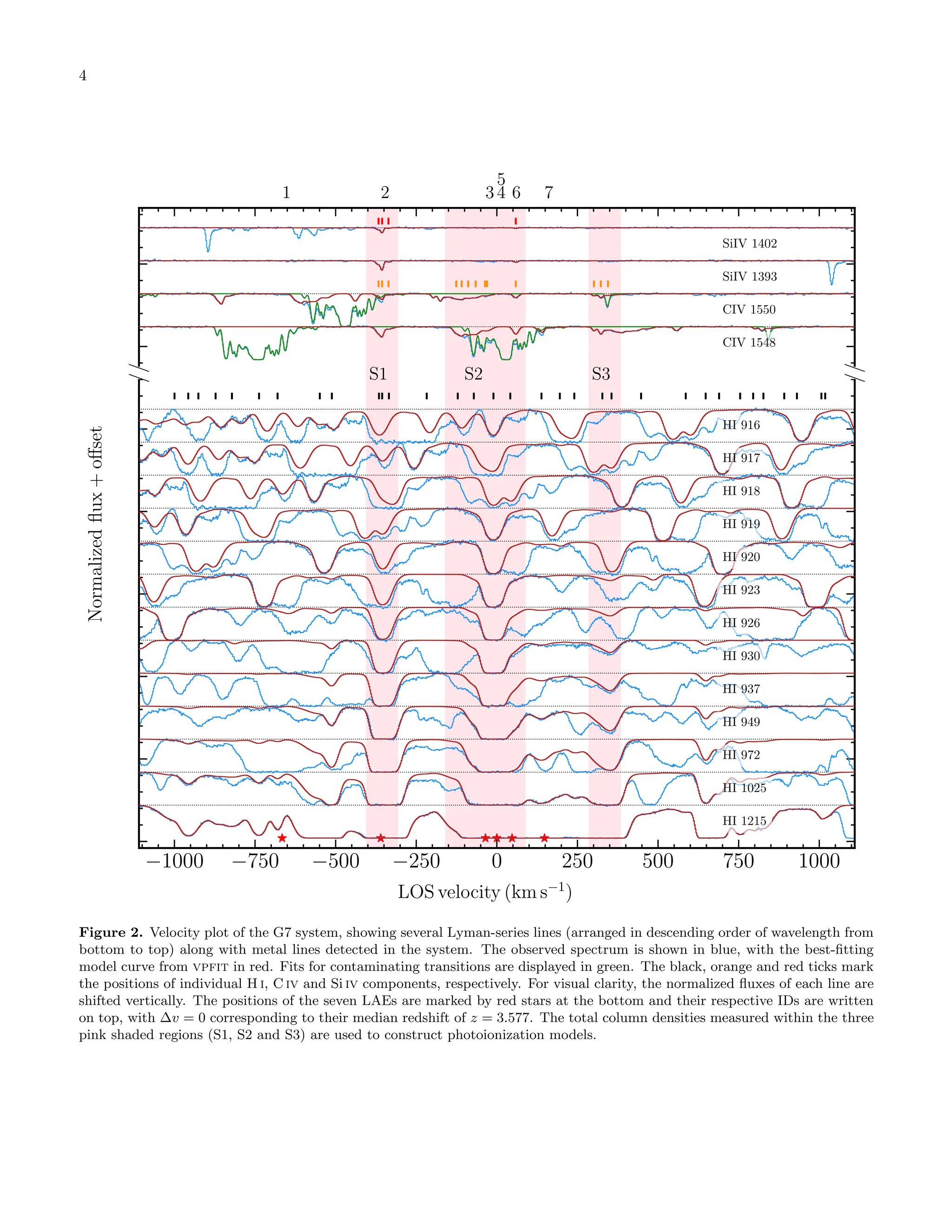
Fig. 2 shows the velocity plot for the Lyman-series
lines and metal transitions associated with the G7 sys-
tem. The seven LAEs are marked by red stars, with
∆v = 0 corresponding to their median redshift of
z = 3.577. To constrain the H i absorber parame-
ters, we simultaneously fitted the Lyman-series lines,
from Lyα to H i-λ916, using the Voigt profile fitting
software vpfit (Carswell & Webb 2014). This soft-
ware minimizes χ2
to determine the best-fitting red-
shift (z), Doppler parameter (b), and column density
(N) of the absorbers. Strong, un-fitted absorption in
higher-order lines is contamination, as evident from the
lack of stronger absorption in Lyα at similar veloci-
ties. This underscores the need for simultaneous fit-
ting of all Lyman-series lines. We identified over 30 H i
components within ±1000 km s−1
, including two pLLSs
at −60 and −300 km s−1
with H i column densities of
log10 N/cm−2
= 16.7 and 16.3, respectively.
Next, we searched for metal transitions associated
with G7 within the same velocity range. We detected
metal absorption corresponding to H i absorbers at ap-
proximately −300, −60, and 300 km s−1
, which we la-
beled as S1, S2, and S3, respectively. The highlighted
velocity ranges used to associate aligned transitions were
based on the structure of the detected metal absorption
lines. C iv absorption was observed in all three systems,
while Si iv was detected in S1 and S2. No other metal
transitions were detected within this range. For non-
detections, we calculated 3σ limiting column densities
using the 3σ limiting equivalent width (Hellsten et al.
1998), assuming the linear part of the curve of growth.
When fitting the aligned C iv and Si iv transitions,
we tied their redshifts. However, the C iv1548 line for
S2 and C iv1550 for S1 are contaminated by Mg ii ab-
sorption from z = 1.52, while C iv1550 in S3 is affected
by a z = 2.83 Al iii line. To accurately measure the
metal absorption parameters, we fitted these contam-
inating lines as well. The N and b of these blended
components are reliably constrained because the corre-
sponding unblended, unsaturated doublet lines provide
accurate measurements. We also excluded transitions
like C iii and Si iii due to heavy contamination from the
Lyα forest.
Among the metal transitions, we identified four pairs
of components (three from S1 and one from S2) where
C iv and Si iv are aligned in redshift. By analyz-
ing the b-parameters of these components, we sepa-
Table 1. Range of the parameters used for Cloudy
Parameter Minimum Maximum Interval
log10 NHI/cm−2
12.5 20.5 0.25
z 2.75 4 0.25
[X/H] -4.0 1.0 0.25
log10 nH/cm−3
-4.5 0.0 0.25
Note:– For the Bayesian inference code, we have used
interpolation to obtain intermediate values.
rated the contributions from temperature (T) and tur-
bulent velocity (vturb) in the medium using the rela-
tion: b2
= v2
turb + 2kBT
mion
. Here, mion is the mass of ion,
kB is the Boltzmann constant and vturb is the turbu-
lent velocity contributing to the non-thermal broaden-
ing. The resulting median temperature of the medium
is log10 (T/K) ≈ 4.7 ± 0.2. While this method can also
be applied using a metal ion and its associated H i ab-
sorber, it was not feasible here due to the presence of
multiple metal absorption components associated with
a single H i absorber.
3.2. Photoionization model
High column density H i absorbers, such as pLLS
and LLS, are typically photoionized across redshifts
(Crighton et al. 2015; Fumagalli et al. 2016b; Prochaska
et al. 2017; Lehner et al. 2018, 2022).
We employed Cloudy (v-C17, Ferland et al. 2013) to
compute ionization corrections, assuming a uniform slab
of gas with a constant hydrogen density (nH) and solar
elemental abundances (Asplund et al. 2009) is in ther-
mal and ionization equilibrium. The incident radiation
is assumed to be the redshift-dependent UV background
(UVB) given by the Haardt & Madau (2001, hereafter,
HM05) model, along with the cosmic microwave back-
ground (CMB). It is important to note that for z > 3,
the UVB models (e.g., HM05, HM12 Haardt & Madau
(2012) or KS18 (Khaire & Srianand 2019)) show mini-
mal variation in the relevant energy range. The model
iterated until it reached the neutral hydrogen column
density (NHi). We did not include dust or grains, as-
suming all elements are in the gas phase.
We applied a Bayesian approach to compare the col-
umn densities and errors of each ion with a grid of pho-
toionization models to derive the metallicities and den-
sities. This method, commonly used in previous studies
(e.g., Fumagalli et al. 2011; Crighton et al. 2015; Lehner
et al. 2018, 2022), is effective in producing robust confi-
dence intervals from posterior probability distributions.
We employed likelihood functions similar to Fumagalli
et al. (2016b). Our model parameters are: (i) neutral
hydrogen column density (NHi), (ii) redshift (z), (iii)](https://image.slidesharecdn.com/2412-250130180325-7ee1c304/75/MUSEQuBES-Unveiling-Cosmic-Web-Filaments-at-z-3-6-through-Dual-Absorption-and-Emission-Line-Analysis-3-2048.jpg)
![5
12
14
16
log
10
(N/cm
−2
)
[X/H] = −1.98+0.14
−0.16
log10 (nH/cm−3
) = −2.65+0.11
−0.10
Model
Data: S1
HI
CIV
SiIV
CII
SiII
AlIII
MgII
−1
0
1
∆
10
12
14
16
log
10
(N/cm
−2
)
[X/H] = −3.69+0.08
−0.08
log10 (nH/cm−3
) = −3.95+0.19
−0.21
Model
Data: S2
HI
CIV
SiIV
CII
SiII
AlIII
MgII
0.0
2.5
∆
8
10
12
14
log
10
(N/cm
−2
)
[X/H] = −2.58+0.13
−0.07
log10 (nH/cm−3
) = −3.81+0.24
−0.31
Model
Data: S3
HI
CIV
CII
SiIV
SiII
AlIII
MgII
0
5
∆
Figure 3. Measured column densities of different transitions
associated with S1, S2 and S3 (top to bottom) are shown in
red, with upper limits indicated by downward arrows. Blue
squares represent the predicted column densities based on
the median values of the model parameters from their re-
spective posterior PDFs. The median values of metallicity
and nH along with their 16th
-84th
percentile ranges are dis-
played at the top. The bottom panel shows the residuals
(∆ ≡ log10 N − log10 Nmodel).
metallicity ([X/H]), and (iv) the total hydrogen number
density (both neutral and ionized), nH = nγ/U, where
nγ is the hydrogen ionizing photon density and U is ion-
ization parameter. The parameter ranges are shown in
table 1.
We used the nested sampling Monte Carlo algorithm
MLFriends implemented in the UltraNest2
package of
Python to obtain the posterior probability density func-
tions (PDFs) of the modeling parameters. Gaussian pri-
ors were adopted for NHi and z based on vpfit con-
straints, while flat priors were used for metallicity and
nH across the grid’s parameter space.
3.3. Results of Photoionization modeling
Fig. 3 compares the observed column densities with
the best-fitting values derived from the medians of the
posterior distributions of model parameters for systems
S1, S2, and S3.
System S1 is closely aligned in velocity with LAE Id 2,
the galaxy nearest to the quasar sightline. Classified as
a pLLS (log10 N/cm−2
= 16.3), it shows C iv and Si iv
detections, with upper limits on C ii, Si ii, Al iii, and
Mg ii. Bayesian analysis with HM05 (KS18) UVB indi-
cates low metallicity, [X/H]= −1.98+0.14
−0.16 (−2.22+0.17
−0.15)
and density log10 nH/cm−3
= −2.65+0.11
−0.10 (−2.94+0.13
−0.11).
System S2 lies near the redshift of the clustered LAEs
and has the highest log10 N/cm−2
= 16.7, also classi-
fied as a pLLS. It shows C iv and weak Si iv detections.
The metallicity of S2 is extremely low, with [X/H]=
−3.69+0.08
−0.08 (HM05) or [X/H]= −4.08+0.08
−0.08 (KS18). The
density is log10 nH/cm−3
= −3.95+0.2
−0.2 (−4.27+0.18
−0.14) for
HM05 (KS18).
System S3 has only C iv detected in addition to H i.
Hence, instead of using flat priors, a Gaussian prior
on density with log10 nH/cm−3
≈ −3.5 ± 0.5, was ap-
plied. This corresponds to the maximum C iv ion-
fraction for the given NHi for the metallicities and red-
shift range included in our grid. This system is also
metal-poor, with [X/H]= −2.58+0.13
−0.07 (−2.94+0.16
−0.13) and
log10 nH/cm−3
= −3.81+0.24
−0.32 (−4.02+0.17
−0.27) using HM05
(KS18) UVB.
4. DISCUSSION AND CONCLUSION
4.1. The G7 system as a tracer of filamentary structure
To assess the overdensity of the G7 system, we used
the LAE luminosity function (LF) to estimate the ex-
pected number of LAEs in a cosmological volume cor-
responding to that of the G7 system. The LF of Drake
et al. (2017) (Herenz et al. 2019) predicts only 0.6 (0.8)
2 https://johannesbuchner.github.io/UltraNest/](https://image.slidesharecdn.com/2412-250130180325-7ee1c304/75/MUSEQuBES-Unveiling-Cosmic-Web-Filaments-at-z-3-6-through-Dual-Absorption-and-Emission-Line-Analysis-5-2048.jpg)
![6
LAEs with log10 (LLyα/erg s−1
) ≥ 41.4, which is the
lowest detected luminosity in the G7 system. Detecting
seven LAEs thus corresponds to a Poisson probability of
3 × 10⁻⁶
(2 × 10⁻⁵
for a mean of 0.8), confirming that
this is a highly overdense region.
The projected spatial distribution of G7 member
LAEs is notably non-random, forming a near-linear
structure (see Fig. 1). Using a Monte Carlo toy model,
we estimated the chance probability of this alignment.
By fitting the pixel coordinates of LAEs with a straight
line3
, we measured the maximum perpendicular distance
(ϵ) from the line. Randomly placing seven points in the
324 × 324 spaxel2
MUSE FoV, we repeated this process
to compute ϵi for 1000 realizations. The probability of
ϵi ≤ ϵ was found to be ≈ 0.3%, indicating that such
alignments are extremely rare.
Five of the seven G7 LAEs (excluding Ids-1 and 2) are
clustered in LOS velocity at z ≈ 3.577, closely matching
the velocity (∆v ≈ −60 km s−1
) of the extremely metal-
poor system S2 ([X/H]= −3.69). These LAEs lie at a
projected distance of 100 − 200 pkpc from the quasar-
sightline. S2, with log10 nH/cm−3
= −4.0 (correspond-
ing to an overdensity of δ ≈ 5; Schaye 2001), likely orig-
inates from cosmic filaments rather than the CGM (e.g.,
Crighton et al. 2013; Fumagalli et al. 2016a,b; Mackenzie
et al. 2019). We therefore investigated whether there are
any traces of extended Lyα emission around this LAE
overdensity.
We reanalyzed the MUSE data using CubEx (Can-
talupo et al. 2019) on the quasar’s point spread func-
tion (PSF) and continuum subtracted cube, focusing
on 5535–5600 Å (±2000 km s−1
from z = 3.577). We
searched for sources with > 3500 connected voxels with
SNR ≥ 1.8. To enhance sensitivity to low-SB sources,
we applied a 4-pixel (0.8′′
) Gaussian spatial smoothing.
This analysis revealed a large extended structure com-
prising > 10000 connected voxels, with a projected lin-
ear size of ≈ 260 pkpc. We confirmed that the structure
spans 16 distinct wavelength layers to ensure the detec-
tion is not spurious.
Fig. 4 displays the SB map (top) of the detected struc-
ture, with the 7 LAEs marked by green squares and
(bottom) the SNR map of the same, overlaid on a sin-
gle wavelength layer associated to the extended emis-
sion. The contours in the middle panel highlights the
SB level of 10−19
erg s−1
cm−2
arcsec−2
, while that on
bottom denotes SNR = 2. Although faint, the detection
is significant as it aligns closely with the LAE positions.
Two LAEs (Ids: 1 and 2) lie directly within the contour,
3 using LinearRegression class from Scikit-learn.
13h
20m
31s
30s
29s
−5◦
230
1500
3000
4500
pos.eq.ra
Dec
(J2000)
G7
50 kpc
1
2
3
4
5
6
7
0.1
0.5
5.0
SB
(×10
−18
c.g.s.)
13h
20m
31s
30s
29s
−5◦
230
1500
3000
4500
R.A. (J2000)
Dec
(J2000)
0.1
2.0
5.0
SNR
Figure 4. Top: The surface brightness (SB) profile of
the extended filament like structure as well as the associ-
ated LAEs of the G7 system. The contour indicates the SB
= 10−19
erg s−1
cm−2
arcsec−2
. Bottom: The SNR map of
the extended emission and the associated LAEs, plotted on
top of a single wavelength layer associated to the extended
emission. The white contours correspond to the SNR of 2. In
both panel, the positions of the seven LAEs are highlighted
by the squares, while the quasar position is marked by a
“x” symbol. Maximum projected length of this structure is
≈ 260 pkpc. Refer to the text for the details about white
dashed and dotted lines.
while two others (Ids: 4 and 7) are just outside it. The
white dashed and dotted lines drawn on top of the SB-
map indicate the best-fit linear alignment of the LAEs
and their maximum deviation, ϵ. The figure shows ex-
cellent correspondence between the extended emission
and the filamentary structure traced by the LAEs.
The absence of emission at the quasar’s location
(marked by the “x”) is likely due to enhanced noise
from PSF subtraction. However, this background source
allows direct measurement of the filament’s nH and
U. Bayesian analysis shows log10 nH/cm−3
ranges be-
tween −4.0 and −2.6 (see Section 3.3), corresponding to
log10 U of −0.8 to −2.2 (for HM05). LAE Id: 2, located](https://image.slidesharecdn.com/2412-250130180325-7ee1c304/75/MUSEQuBES-Unveiling-Cosmic-Web-Filaments-at-z-3-6-through-Dual-Absorption-and-Emission-Line-Analysis-6-2048.jpg)
![Draft version January 10, 2025
Typeset using L
A
TEX twocolumn style in AASTeX631
MUSEQuBES: Unveiling Cosmic Web Filaments at z ≈ 3.6 through Dual Absorption and Emission
Line Analysis
Eshita Banerjee ,1
Sowgat Muzahid ,1
Joop Schaye,2
Sebastiano Cantalupo,3
and Sean D. Johnson4
1IUCAA, Post Bag 04, Ganeshkhind, Pune, India, 411007
2Leiden Observatory, Leiden University, P.O. Box 9513, NL-2300 AA Leiden, the Netherlands
3Department of Physics, University of Milan Bicocca, Piazza della Scienza 3, I-20126 Milano, Italy
4Department of Astronomy, University of Michigan, 1085 S. University, Ann Arbor, MI 48109, USA
ABSTRACT
According to modern cosmological models, galaxies are embedded within cosmic filaments, which sup-
ply a continuous flow of pristine gas, fueling star formation and driving their evolution. However, due to
their low density, the direct detection of diffuse gas in cosmic filaments remains elusive. Here, we report
the discovery of an extremely metal-poor ([X/H] ≈ −3.7), low-density (log10 nH/cm−3
≈ −4, corre-
sponding to an overdensity of ≈ 5) partial Lyman limit system (pLLS) at z ≈ 3.577 along the quasar
sightline Q1317–0507, probing cosmic filaments. Additionally, two other low-metallicity ([X/H]≲ −2)
absorption systems are detected at similar redshifts, one of which is also a pLLS. VLT/MUSE obser-
vations reveal a significant overdensity of Lyα emitters (LAEs) associated with these absorbers. The
spatial distribution of the LAEs strongly suggests the presence of an underlying filamentary structure.
This is further supported by the detection of a large Lyα emitting nebula with a surface brightness of
≥ 10−19
erg cm−2
s−1
arcsec−2
, with a maximum projected linear size of ≈ 260 pkpc extending along
the LAEs. This is the first detection of giant Lyα emission tracing cosmic filaments, linked to normal
galaxies and likely powered by in-situ recombination.
Keywords: galaxies: evolution — galaxies: high-redshift — (galaxies:) quasars: absorption lines
1. INTRODUCTION
In the current cosmological framework, galaxies
emerge within the dense intersections of the cosmic
web—a large-scale network of dark matter halos and
filaments that span the universe. These structures chan-
nel gas from the intergalactic medium (IGM) into dark
matter halos, where it eventually cools, triggering star
formation. However, detecting these emission from the
gas in elusive filaments is challenging due to their low
densities.
Recent advancements in integral field units (IFUs)
with large fields of view, like MUSE (Bacon et al. 2010),
have revolutionized our ability to detect these filament-
like structures, glowing in Lyα -emission at high red-
shifts (Fumagalli et al. 2016b; Bacon et al. 2021; Johnson
et al. 2022; Tornotti et al. 2024a). These observations
Corresponding author: Eshita Banerjee, Sowgat Muzahid
eshitaban18@iucaa.in, sowgat@iucaa.in
offer new insights into gas flow from the IGM into galax-
ies, particularly through “cold-mode accretion” (e.g.,
Kereš et al. 2005), where gas is funneled into galaxies
via narrow, dense filaments. This process significantly
contributes to the optically thick gas associated with
Lyman-limit systems (LLSs: log10(NHi) > 17.2) (see,
Fumagalli et al. 2011; van de Voort et al. 2012).
Fumagalli et al. (2013) have shown that while gas
in galaxy halos can account for all LLSs at z < 3,
at z ≳ 3.5, the contribution of the IGM to LLSs be-
comes pronounced, as the overdensities associated with
these systems decrease (see, Schaye 2001) and the ex-
tragalactic UV background (UVB) weakens, enhancing
gas shielding. Consequently, LLSs are considered effec-
tive tracers of cold-stream inflows onto galaxies, often
identified by their low metallicity (e.g., Ribaudo et al.
2011; Crighton et al. 2013) or filamentary morphology
(e.g., Fumagalli et al. 2016b). At z ≈ 3, only a small
fraction (≈ 18%) of LLSs and partial-LLSs (pLLSs:
16.2 < log10(NHi) < 17.2) are extremely metal-poor,
arXiv:2412.04546v2
[astro-ph.GA]
9
Jan
2025](https://crownmelresort.com/image.slidesharecdn.com/2412-250130180325-7ee1c304/75/MUSEQuBES-Unveiling-Cosmic-Web-Filaments-at-z-3-6-through-Dual-Absorption-and-Emission-Line-Analysis-1-2048.jpg)
![2
with metallicity being [X/H]< −3 (Lehner et al. 2016,
2022; Lofthouse et al. 2023).
Interestingly, in our MUSEQuBES survey, we identi-
fied an overdensity of Lyα emitters (LAEs) at z ≈ 3.577,
consisting of seven LAEs arranged in an almost linear
configuration. Suspecting a filament connecting these
LAEs, we explored potential inflow signatures by mod-
eling absorbers probed by a background quasar and
searched for extended emission around this structure.
This investigation revealed a low-metallicity absorption
system and a coincident giant Lyα nebula. This letter
is organized as follows: section 2 introduces our data;
section 3 presents absorption measurements and model-
ing, and finally, we summarize our study and discuss the
results in section 4. We adopt a flat ΛCDM cosmology
with H0 = 70 km s−1
Mpc−1
, ΩM = 0.3 and ΩΛ = 0.7.
Metallicity is expressed as log10(Z/Z⊙) ≡[X/H], where
Z⊙ is the solar metallicity (= 0.013; see Grevesse et al.
(2012)). Distances are in physical kpc (hereafter, pkpc)
unless specified otherwise.
2. DATA
The LAE overdensity analyzed in this study is de-
tected toward the quasar Q1317−0507, observed as part
of the MUSEQuBES survey (Muzahid et al. 2020, 2021;
Banerjee et al. 2023, 2024). We obtained 10 hours of on-
source VLT/MUSE observations with an effective seeing
of < 0.6
′′
. The final data cube has a spatial sampling of
0.2
′′
×0.2
′′
per pixel, and a spectral resolution of ≈ 3600
(FWHM ≈ 86 km s−1
) in the optical range (4750–9350
Å). The data reduction process is comprehensively de-
scribed in Muzahid et al. (2021).
Complementary to the MUSE data, we utilized a
high-resolution optical spectrum of the quasar from
VLT/UVES (R ≈ 45, 000), sourced from the SQUAD
database (Murphy et al. 2019). The coadded and
continuum-normalized spectrum provides a median
signal-to-noise ratio (SNR) of 35 within the Lyα -forest
region and 80 redward of the quasar’s Lyα emission.
Additionally, we incorporated near-infrared data from
VLT/X-shooter, covering 1000-2480 nm with a spectral
resolution of R ≈ 5300 and a median SNR of ≈ 35. This
spectrum, along with its best-fitting continuum, were re-
trieved from the ESO data archive (López et al. 2016).
3. ANALYSIS AND RESULTS
Muzahid et al. (2020) identified 22 LAEs in the MUSE
field centered on the background quasar Q1317−0507
(zqso = 3.7) in the redshift range 2.9 < z < 3.6. These
LAEs were detected based on their Lyα emission lines,
which typically show offsets of hundreds of km s−1
from
the systemic redshifts (e.g., Steidel et al. 2010; Rakic
3.566 3.568 3.570 3.572 3.574 3.576 3.578
zLAE
0
2
Count
1 2 3 4
5 6 7
13h
20m
32s
31s
30s
29s
28s
−5◦
230
1500
3000
4500
240
0000
R.A. (J2000)
Dec
(J2000)
G7
1
2
3
4
5
6
7
0.1
0.5
5.0
SB
(×10
−18
erg
s
−1
cm
−2
arcsec
−2
)
Figure 1. The optimally extracted Lyα surface brightness
maps of the 7 LAEs (G7) within the MUSE FOV centered
on the quasar Q1317−0507 (marked by the “+” sign). The
pixels within the 3D segmentation map for each LAE are
combined and projected onto the image, with the gray con-
tours representing the 5 and 25 σ from the mean flux levels of
the continuum-bright objects. A Gaussian smoothing func-
tion with σ = 0.2′′
(≡ 1 pixel) has been applied to enhance
visual clarity of the SB map. The histogram in top panel dis-
plays the redshift distribution of the LAEs. The object IDs
are indicated beside each LAEs as well as in the histogram
plot.
et al. 2011; Shibuya et al. 2014; Verhamme et al. 2018).
The Lyα redshifts were corrected using the empirical
relation from Muzahid et al. (2020). A friends-of-friends
algorithm, using a linking velocity1
of 500 km s−1
along
the line of sight (LOS), identified a galaxy overdensity
with 7 LAEs at z ≈ 3.57, making it the most LAE-rich
system in the MUSEQuBES sample.
Figure 1 shows the optimally extracted Lyα surface
brightness (SB) map of this overdense region (hereafter,
G7). The redshifts of the seven LAEs range from z ≈
3.566 to 3.578. The LAE closest to the quasar-sightline
is Id:2, at a transverse distance of 34 pkpc, followed by
Id:3 at 91 pkpc. The other LAEs are located beyond
100 pkpc, with the farthest at 220 pkpc. The redshift
histogram reveals that five of the seven LAEs (excluding
1 earlier, Muzahid et al. (2021) also used the similar velocity win-
dow for defining galaxy-groups.](https://crownmelresort.com/image.slidesharecdn.com/2412-250130180325-7ee1c304/75/MUSEQuBES-Unveiling-Cosmic-Web-Filaments-at-z-3-6-through-Dual-Absorption-and-Emission-Line-Analysis-2-2048.jpg)
![3
Id:1 and Id:2) are tightly clustered at z ≈ 3.577, which is
≈ 8000 km s−1
or 20 pMpc from the background quasar.
3.1. Measurements of absorption lines associated with
G7
Fig. 2 shows the velocity plot for the Lyman-series
lines and metal transitions associated with the G7 sys-
tem. The seven LAEs are marked by red stars, with
∆v = 0 corresponding to their median redshift of
z = 3.577. To constrain the H i absorber parame-
ters, we simultaneously fitted the Lyman-series lines,
from Lyα to H i-λ916, using the Voigt profile fitting
software vpfit (Carswell & Webb 2014). This soft-
ware minimizes χ2
to determine the best-fitting red-
shift (z), Doppler parameter (b), and column density
(N) of the absorbers. Strong, un-fitted absorption in
higher-order lines is contamination, as evident from the
lack of stronger absorption in Lyα at similar veloci-
ties. This underscores the need for simultaneous fit-
ting of all Lyman-series lines. We identified over 30 H i
components within ±1000 km s−1
, including two pLLSs
at −60 and −300 km s−1
with H i column densities of
log10 N/cm−2
= 16.7 and 16.3, respectively.
Next, we searched for metal transitions associated
with G7 within the same velocity range. We detected
metal absorption corresponding to H i absorbers at ap-
proximately −300, −60, and 300 km s−1
, which we la-
beled as S1, S2, and S3, respectively. The highlighted
velocity ranges used to associate aligned transitions were
based on the structure of the detected metal absorption
lines. C iv absorption was observed in all three systems,
while Si iv was detected in S1 and S2. No other metal
transitions were detected within this range. For non-
detections, we calculated 3σ limiting column densities
using the 3σ limiting equivalent width (Hellsten et al.
1998), assuming the linear part of the curve of growth.
When fitting the aligned C iv and Si iv transitions,
we tied their redshifts. However, the C iv1548 line for
S2 and C iv1550 for S1 are contaminated by Mg ii ab-
sorption from z = 1.52, while C iv1550 in S3 is affected
by a z = 2.83 Al iii line. To accurately measure the
metal absorption parameters, we fitted these contam-
inating lines as well. The N and b of these blended
components are reliably constrained because the corre-
sponding unblended, unsaturated doublet lines provide
accurate measurements. We also excluded transitions
like C iii and Si iii due to heavy contamination from the
Lyα forest.
Among the metal transitions, we identified four pairs
of components (three from S1 and one from S2) where
C iv and Si iv are aligned in redshift. By analyz-
ing the b-parameters of these components, we sepa-
Table 1. Range of the parameters used for Cloudy
Parameter Minimum Maximum Interval
log10 NHI/cm−2
12.5 20.5 0.25
z 2.75 4 0.25
[X/H] -4.0 1.0 0.25
log10 nH/cm−3
-4.5 0.0 0.25
Note:– For the Bayesian inference code, we have used
interpolation to obtain intermediate values.
rated the contributions from temperature (T) and tur-
bulent velocity (vturb) in the medium using the rela-
tion: b2
= v2
turb + 2kBT
mion
. Here, mion is the mass of ion,
kB is the Boltzmann constant and vturb is the turbu-
lent velocity contributing to the non-thermal broaden-
ing. The resulting median temperature of the medium
is log10 (T/K) ≈ 4.7 ± 0.2. While this method can also
be applied using a metal ion and its associated H i ab-
sorber, it was not feasible here due to the presence of
multiple metal absorption components associated with
a single H i absorber.
3.2. Photoionization model
High column density H i absorbers, such as pLLS
and LLS, are typically photoionized across redshifts
(Crighton et al. 2015; Fumagalli et al. 2016b; Prochaska
et al. 2017; Lehner et al. 2018, 2022).
We employed Cloudy (v-C17, Ferland et al. 2013) to
compute ionization corrections, assuming a uniform slab
of gas with a constant hydrogen density (nH) and solar
elemental abundances (Asplund et al. 2009) is in ther-
mal and ionization equilibrium. The incident radiation
is assumed to be the redshift-dependent UV background
(UVB) given by the Haardt & Madau (2001, hereafter,
HM05) model, along with the cosmic microwave back-
ground (CMB). It is important to note that for z > 3,
the UVB models (e.g., HM05, HM12 Haardt & Madau
(2012) or KS18 (Khaire & Srianand 2019)) show mini-
mal variation in the relevant energy range. The model
iterated until it reached the neutral hydrogen column
density (NHi). We did not include dust or grains, as-
suming all elements are in the gas phase.
We applied a Bayesian approach to compare the col-
umn densities and errors of each ion with a grid of pho-
toionization models to derive the metallicities and den-
sities. This method, commonly used in previous studies
(e.g., Fumagalli et al. 2011; Crighton et al. 2015; Lehner
et al. 2018, 2022), is effective in producing robust confi-
dence intervals from posterior probability distributions.
We employed likelihood functions similar to Fumagalli
et al. (2016b). Our model parameters are: (i) neutral
hydrogen column density (NHi), (ii) redshift (z), (iii)](https://crownmelresort.com/image.slidesharecdn.com/2412-250130180325-7ee1c304/75/MUSEQuBES-Unveiling-Cosmic-Web-Filaments-at-z-3-6-through-Dual-Absorption-and-Emission-Line-Analysis-3-2048.jpg)

![5
12
14
16
log
10
(N/cm
−2
)
[X/H] = −1.98+0.14
−0.16
log10 (nH/cm−3
) = −2.65+0.11
−0.10
Model
Data: S1
HI
CIV
SiIV
CII
SiII
AlIII
MgII
−1
0
1
∆
10
12
14
16
log
10
(N/cm
−2
)
[X/H] = −3.69+0.08
−0.08
log10 (nH/cm−3
) = −3.95+0.19
−0.21
Model
Data: S2
HI
CIV
SiIV
CII
SiII
AlIII
MgII
0.0
2.5
∆
8
10
12
14
log
10
(N/cm
−2
)
[X/H] = −2.58+0.13
−0.07
log10 (nH/cm−3
) = −3.81+0.24
−0.31
Model
Data: S3
HI
CIV
CII
SiIV
SiII
AlIII
MgII
0
5
∆
Figure 3. Measured column densities of different transitions
associated with S1, S2 and S3 (top to bottom) are shown in
red, with upper limits indicated by downward arrows. Blue
squares represent the predicted column densities based on
the median values of the model parameters from their re-
spective posterior PDFs. The median values of metallicity
and nH along with their 16th
-84th
percentile ranges are dis-
played at the top. The bottom panel shows the residuals
(∆ ≡ log10 N − log10 Nmodel).
metallicity ([X/H]), and (iv) the total hydrogen number
density (both neutral and ionized), nH = nγ/U, where
nγ is the hydrogen ionizing photon density and U is ion-
ization parameter. The parameter ranges are shown in
table 1.
We used the nested sampling Monte Carlo algorithm
MLFriends implemented in the UltraNest2
package of
Python to obtain the posterior probability density func-
tions (PDFs) of the modeling parameters. Gaussian pri-
ors were adopted for NHi and z based on vpfit con-
straints, while flat priors were used for metallicity and
nH across the grid’s parameter space.
3.3. Results of Photoionization modeling
Fig. 3 compares the observed column densities with
the best-fitting values derived from the medians of the
posterior distributions of model parameters for systems
S1, S2, and S3.
System S1 is closely aligned in velocity with LAE Id 2,
the galaxy nearest to the quasar sightline. Classified as
a pLLS (log10 N/cm−2
= 16.3), it shows C iv and Si iv
detections, with upper limits on C ii, Si ii, Al iii, and
Mg ii. Bayesian analysis with HM05 (KS18) UVB indi-
cates low metallicity, [X/H]= −1.98+0.14
−0.16 (−2.22+0.17
−0.15)
and density log10 nH/cm−3
= −2.65+0.11
−0.10 (−2.94+0.13
−0.11).
System S2 lies near the redshift of the clustered LAEs
and has the highest log10 N/cm−2
= 16.7, also classi-
fied as a pLLS. It shows C iv and weak Si iv detections.
The metallicity of S2 is extremely low, with [X/H]=
−3.69+0.08
−0.08 (HM05) or [X/H]= −4.08+0.08
−0.08 (KS18). The
density is log10 nH/cm−3
= −3.95+0.2
−0.2 (−4.27+0.18
−0.14) for
HM05 (KS18).
System S3 has only C iv detected in addition to H i.
Hence, instead of using flat priors, a Gaussian prior
on density with log10 nH/cm−3
≈ −3.5 ± 0.5, was ap-
plied. This corresponds to the maximum C iv ion-
fraction for the given NHi for the metallicities and red-
shift range included in our grid. This system is also
metal-poor, with [X/H]= −2.58+0.13
−0.07 (−2.94+0.16
−0.13) and
log10 nH/cm−3
= −3.81+0.24
−0.32 (−4.02+0.17
−0.27) using HM05
(KS18) UVB.
4. DISCUSSION AND CONCLUSION
4.1. The G7 system as a tracer of filamentary structure
To assess the overdensity of the G7 system, we used
the LAE luminosity function (LF) to estimate the ex-
pected number of LAEs in a cosmological volume cor-
responding to that of the G7 system. The LF of Drake
et al. (2017) (Herenz et al. 2019) predicts only 0.6 (0.8)
2 https://johannesbuchner.github.io/UltraNest/](https://crownmelresort.com/image.slidesharecdn.com/2412-250130180325-7ee1c304/75/MUSEQuBES-Unveiling-Cosmic-Web-Filaments-at-z-3-6-through-Dual-Absorption-and-Emission-Line-Analysis-5-2048.jpg)
![6
LAEs with log10 (LLyα/erg s−1
) ≥ 41.4, which is the
lowest detected luminosity in the G7 system. Detecting
seven LAEs thus corresponds to a Poisson probability of
3 × 10⁻⁶
(2 × 10⁻⁵
for a mean of 0.8), confirming that
this is a highly overdense region.
The projected spatial distribution of G7 member
LAEs is notably non-random, forming a near-linear
structure (see Fig. 1). Using a Monte Carlo toy model,
we estimated the chance probability of this alignment.
By fitting the pixel coordinates of LAEs with a straight
line3
, we measured the maximum perpendicular distance
(ϵ) from the line. Randomly placing seven points in the
324 × 324 spaxel2
MUSE FoV, we repeated this process
to compute ϵi for 1000 realizations. The probability of
ϵi ≤ ϵ was found to be ≈ 0.3%, indicating that such
alignments are extremely rare.
Five of the seven G7 LAEs (excluding Ids-1 and 2) are
clustered in LOS velocity at z ≈ 3.577, closely matching
the velocity (∆v ≈ −60 km s−1
) of the extremely metal-
poor system S2 ([X/H]= −3.69). These LAEs lie at a
projected distance of 100 − 200 pkpc from the quasar-
sightline. S2, with log10 nH/cm−3
= −4.0 (correspond-
ing to an overdensity of δ ≈ 5; Schaye 2001), likely orig-
inates from cosmic filaments rather than the CGM (e.g.,
Crighton et al. 2013; Fumagalli et al. 2016a,b; Mackenzie
et al. 2019). We therefore investigated whether there are
any traces of extended Lyα emission around this LAE
overdensity.
We reanalyzed the MUSE data using CubEx (Can-
talupo et al. 2019) on the quasar’s point spread func-
tion (PSF) and continuum subtracted cube, focusing
on 5535–5600 Å (±2000 km s−1
from z = 3.577). We
searched for sources with > 3500 connected voxels with
SNR ≥ 1.8. To enhance sensitivity to low-SB sources,
we applied a 4-pixel (0.8′′
) Gaussian spatial smoothing.
This analysis revealed a large extended structure com-
prising > 10000 connected voxels, with a projected lin-
ear size of ≈ 260 pkpc. We confirmed that the structure
spans 16 distinct wavelength layers to ensure the detec-
tion is not spurious.
Fig. 4 displays the SB map (top) of the detected struc-
ture, with the 7 LAEs marked by green squares and
(bottom) the SNR map of the same, overlaid on a sin-
gle wavelength layer associated to the extended emis-
sion. The contours in the middle panel highlights the
SB level of 10−19
erg s−1
cm−2
arcsec−2
, while that on
bottom denotes SNR = 2. Although faint, the detection
is significant as it aligns closely with the LAE positions.
Two LAEs (Ids: 1 and 2) lie directly within the contour,
3 using LinearRegression class from Scikit-learn.
13h
20m
31s
30s
29s
−5◦
230
1500
3000
4500
pos.eq.ra
Dec
(J2000)
G7
50 kpc
1
2
3
4
5
6
7
0.1
0.5
5.0
SB
(×10
−18
c.g.s.)
13h
20m
31s
30s
29s
−5◦
230
1500
3000
4500
R.A. (J2000)
Dec
(J2000)
0.1
2.0
5.0
SNR
Figure 4. Top: The surface brightness (SB) profile of
the extended filament like structure as well as the associ-
ated LAEs of the G7 system. The contour indicates the SB
= 10−19
erg s−1
cm−2
arcsec−2
. Bottom: The SNR map of
the extended emission and the associated LAEs, plotted on
top of a single wavelength layer associated to the extended
emission. The white contours correspond to the SNR of 2. In
both panel, the positions of the seven LAEs are highlighted
by the squares, while the quasar position is marked by a
“x” symbol. Maximum projected length of this structure is
≈ 260 pkpc. Refer to the text for the details about white
dashed and dotted lines.
while two others (Ids: 4 and 7) are just outside it. The
white dashed and dotted lines drawn on top of the SB-
map indicate the best-fit linear alignment of the LAEs
and their maximum deviation, ϵ. The figure shows ex-
cellent correspondence between the extended emission
and the filamentary structure traced by the LAEs.
The absence of emission at the quasar’s location
(marked by the “x”) is likely due to enhanced noise
from PSF subtraction. However, this background source
allows direct measurement of the filament’s nH and
U. Bayesian analysis shows log10 nH/cm−3
ranges be-
tween −4.0 and −2.6 (see Section 3.3), corresponding to
log10 U of −0.8 to −2.2 (for HM05). LAE Id: 2, located](https://crownmelresort.com/image.slidesharecdn.com/2412-250130180325-7ee1c304/75/MUSEQuBES-Unveiling-Cosmic-Web-Filaments-at-z-3-6-through-Dual-Absorption-and-Emission-Line-Analysis-6-2048.jpg)


This document discusses the detection of cosmic web filaments at redshift z ≈ 3.6, revealing an extremely metal-poor partial Lyman limit system linked to galaxies and characterized by significant Lyman-alpha emission. The study employs advanced observational technologies to trace cosmic gas flows and identifies a notable overdensity of Lyman-alpha emitters, suggesting active star formation within these filaments. The findings contribute to a deeper understanding of galaxy evolution and the structure of the universe's large-scale networks.


