Downloaded 1,024 times


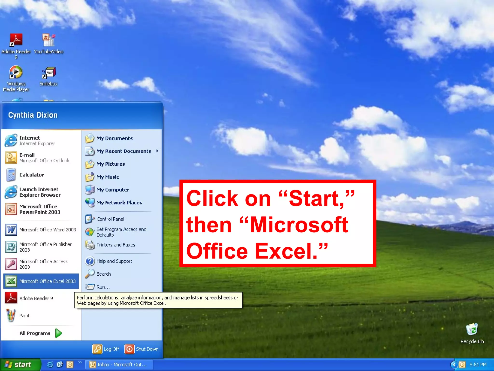
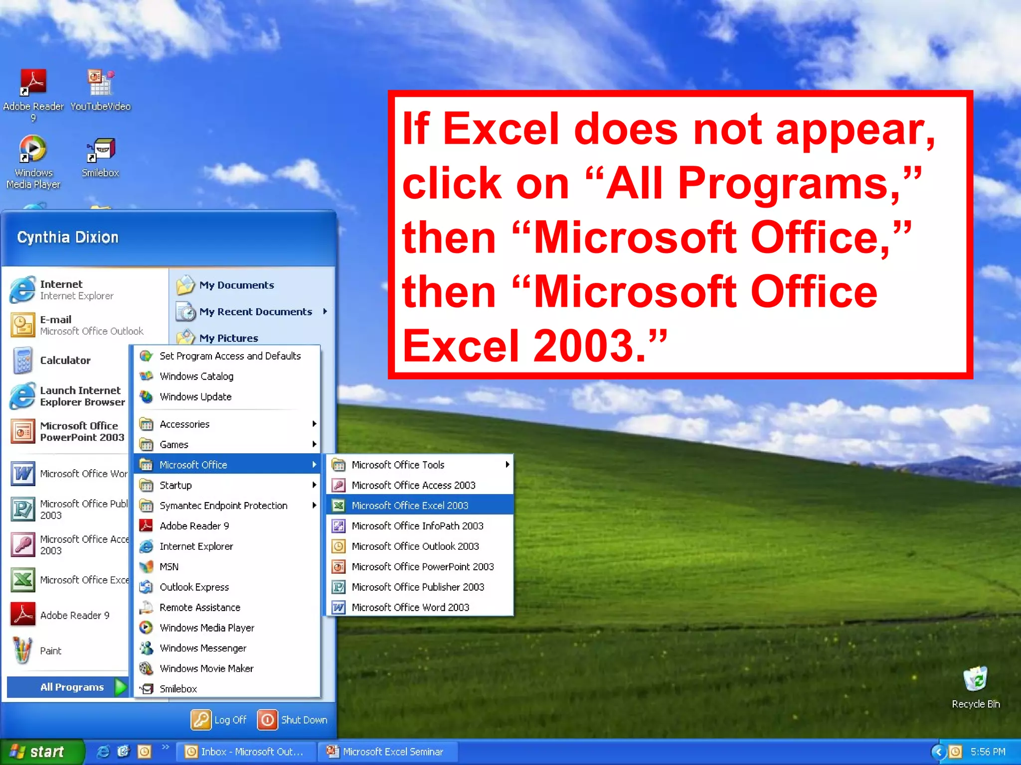
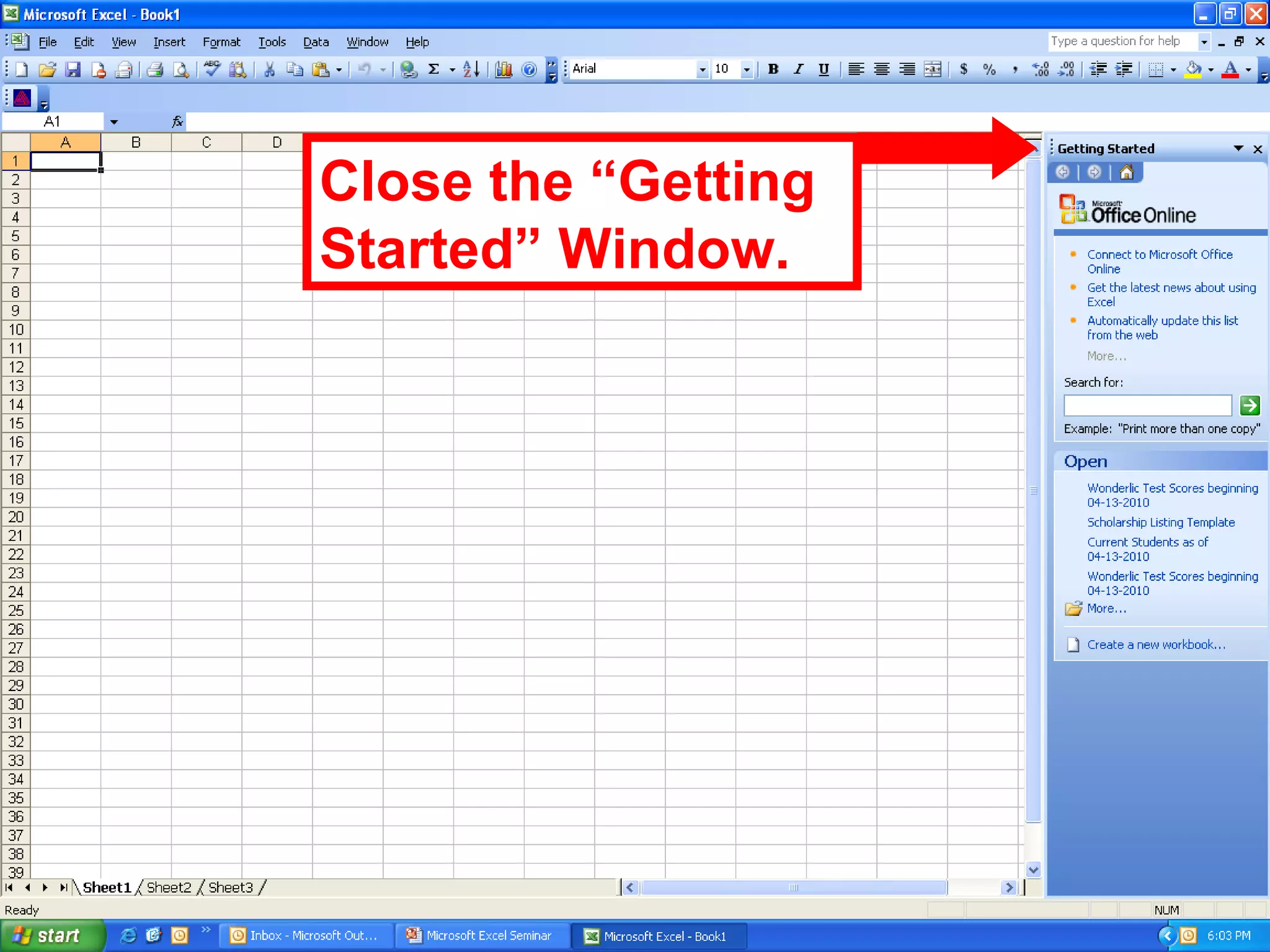
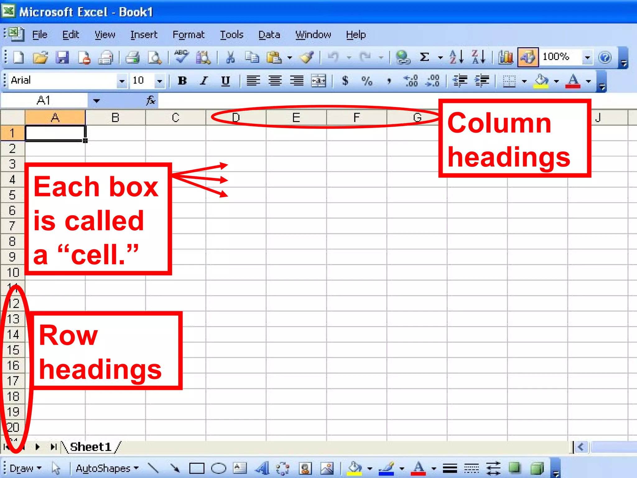
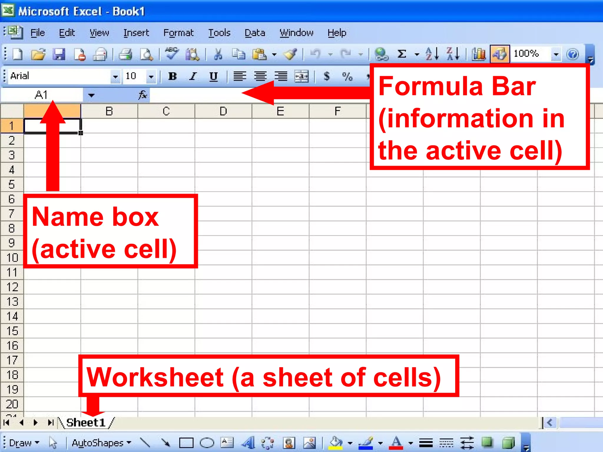
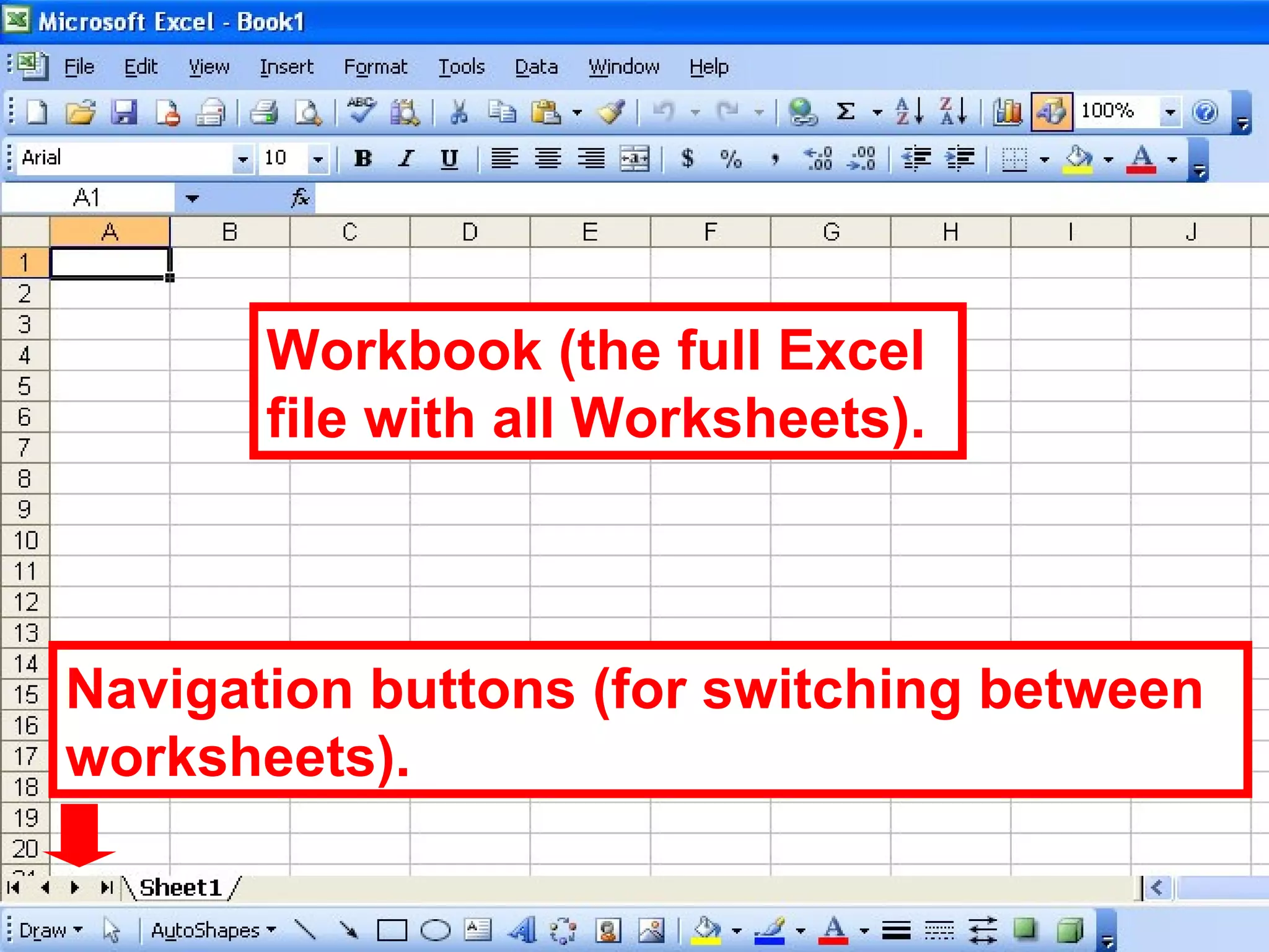
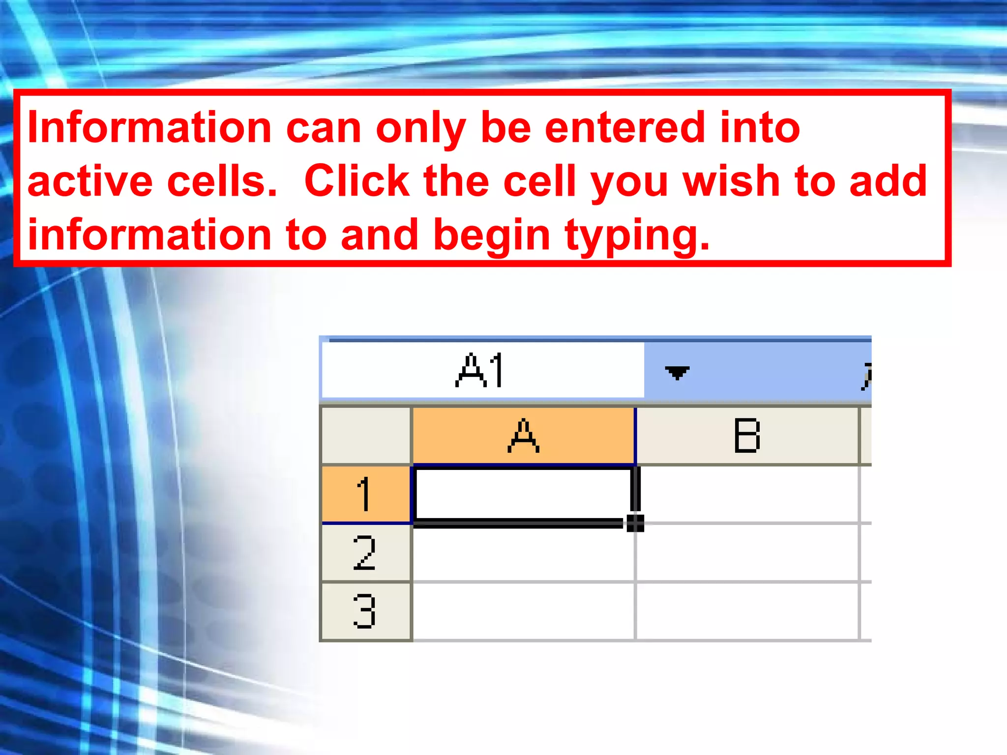
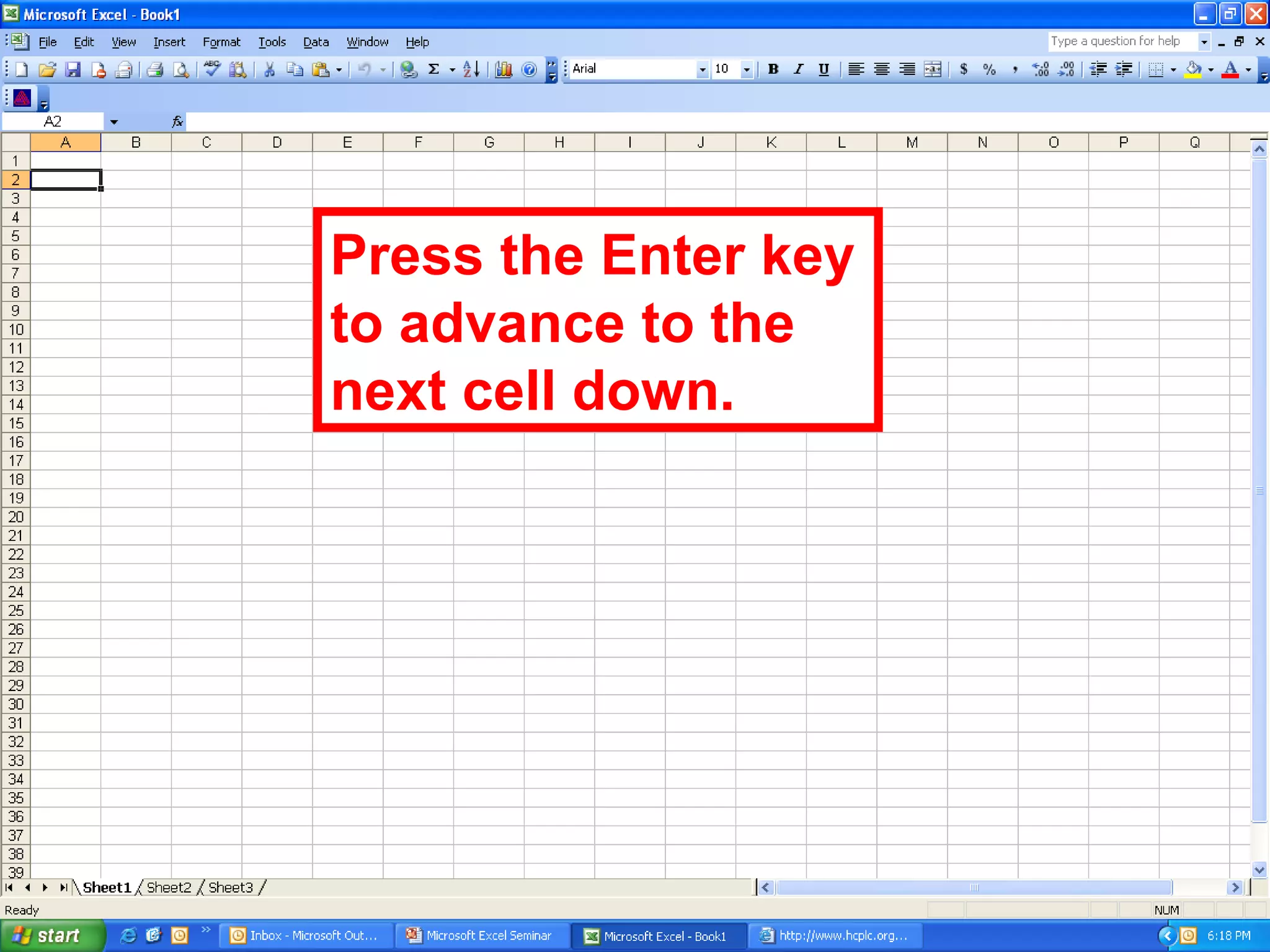
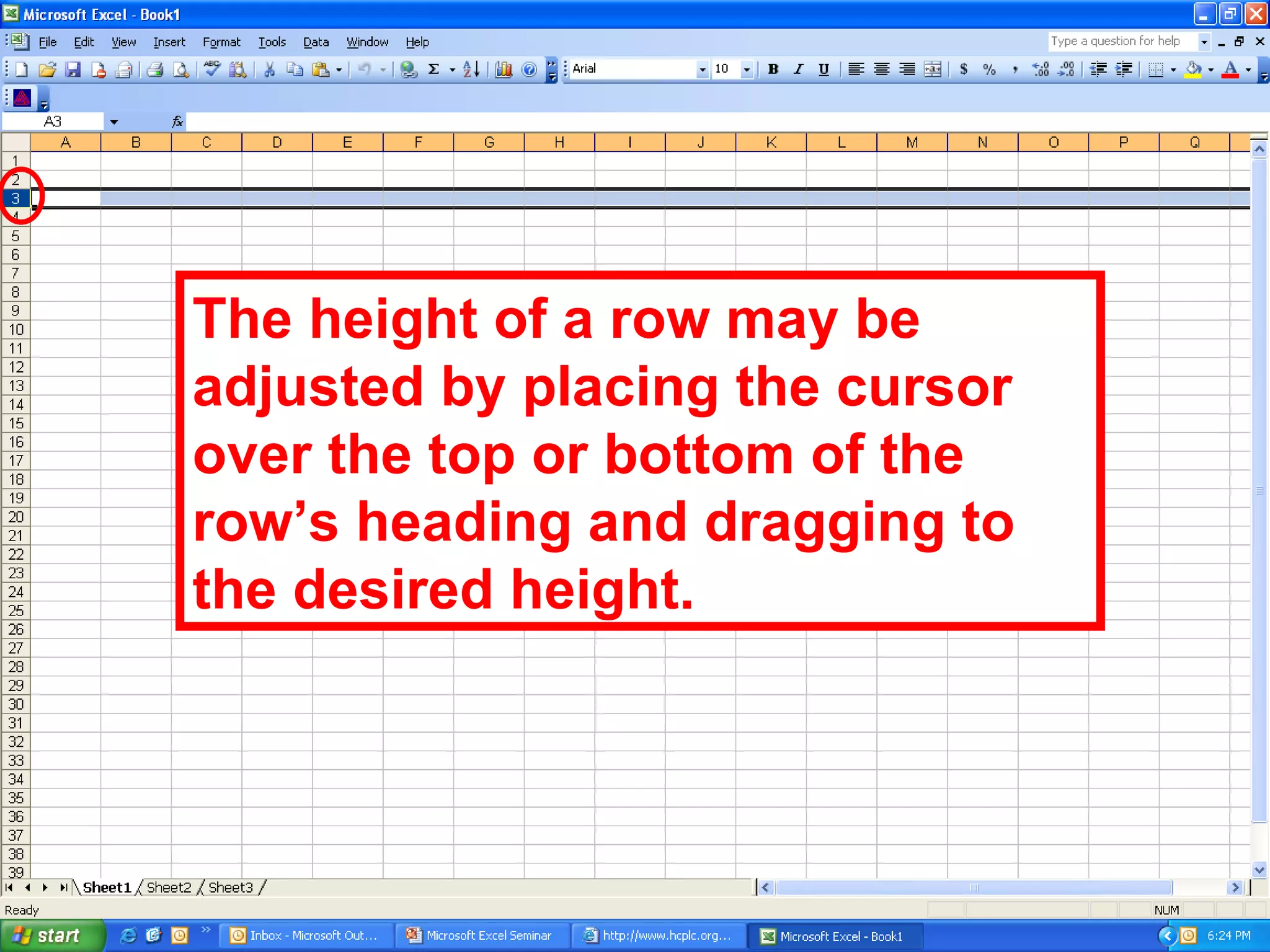
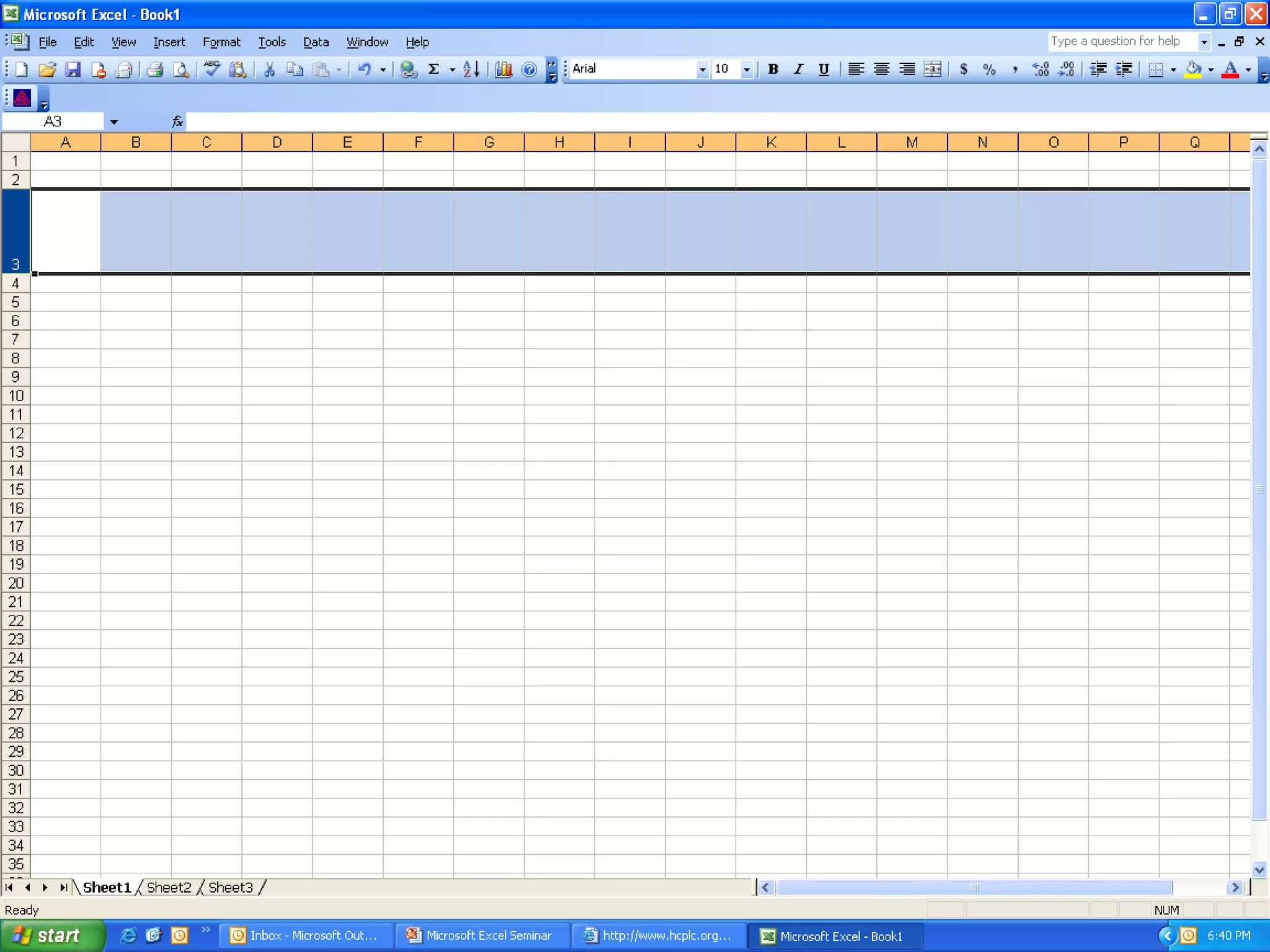
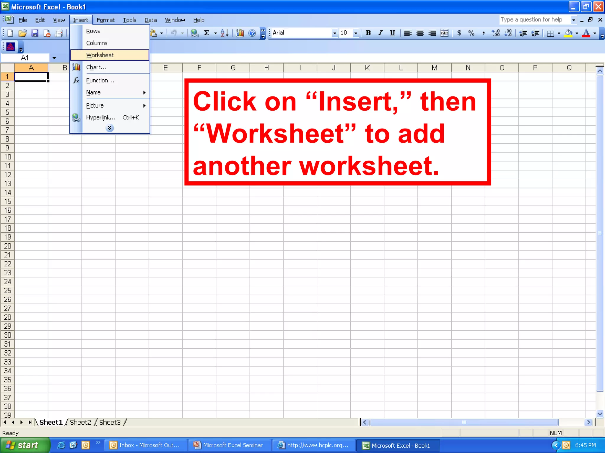
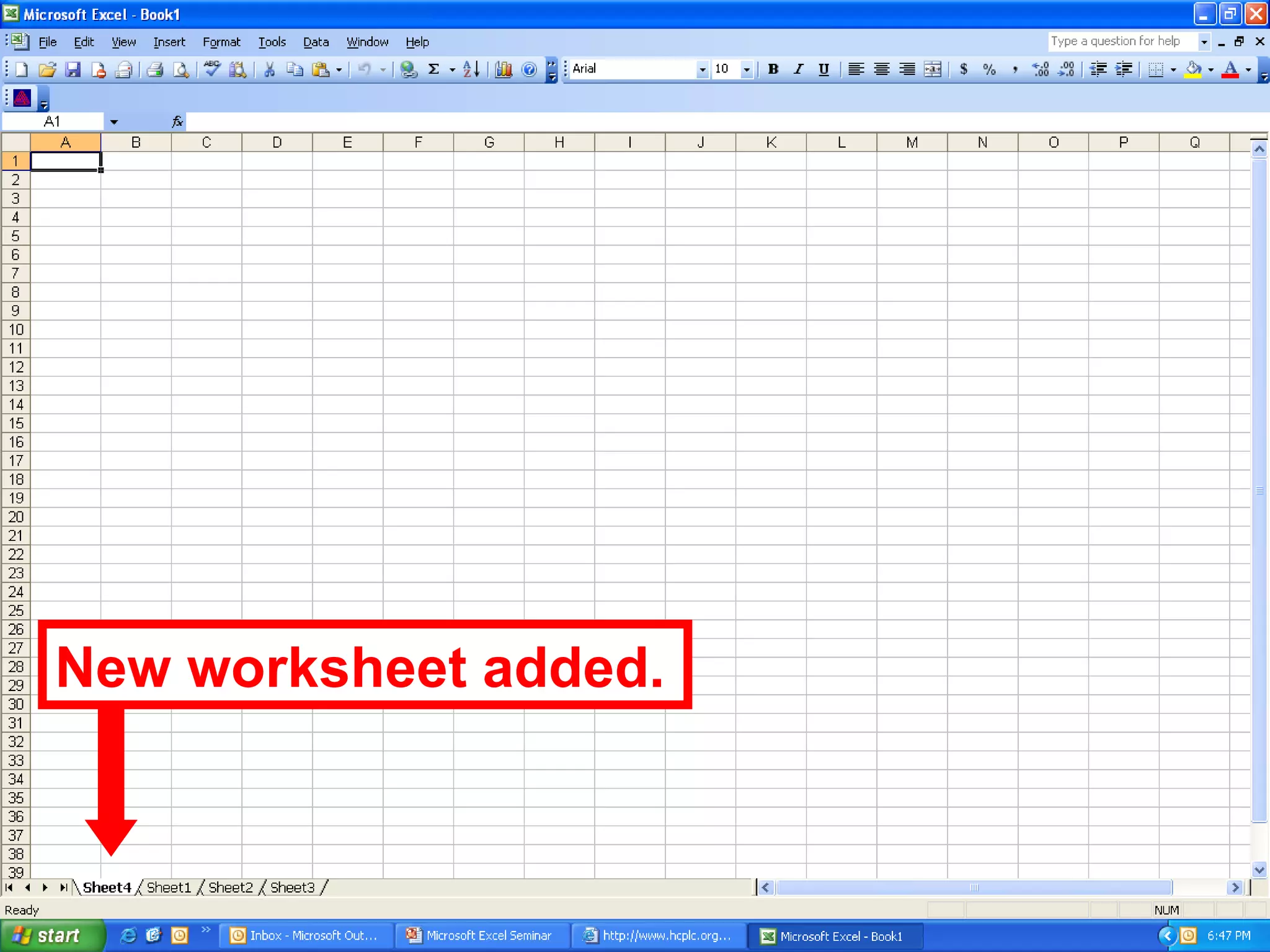
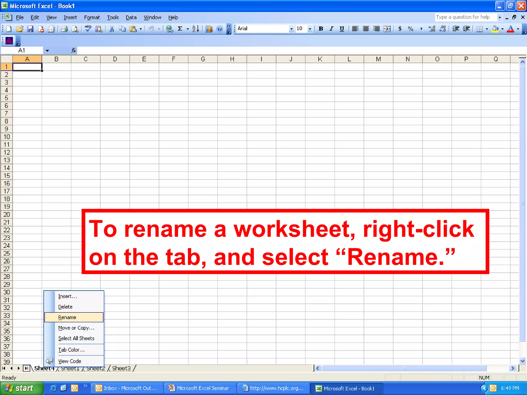
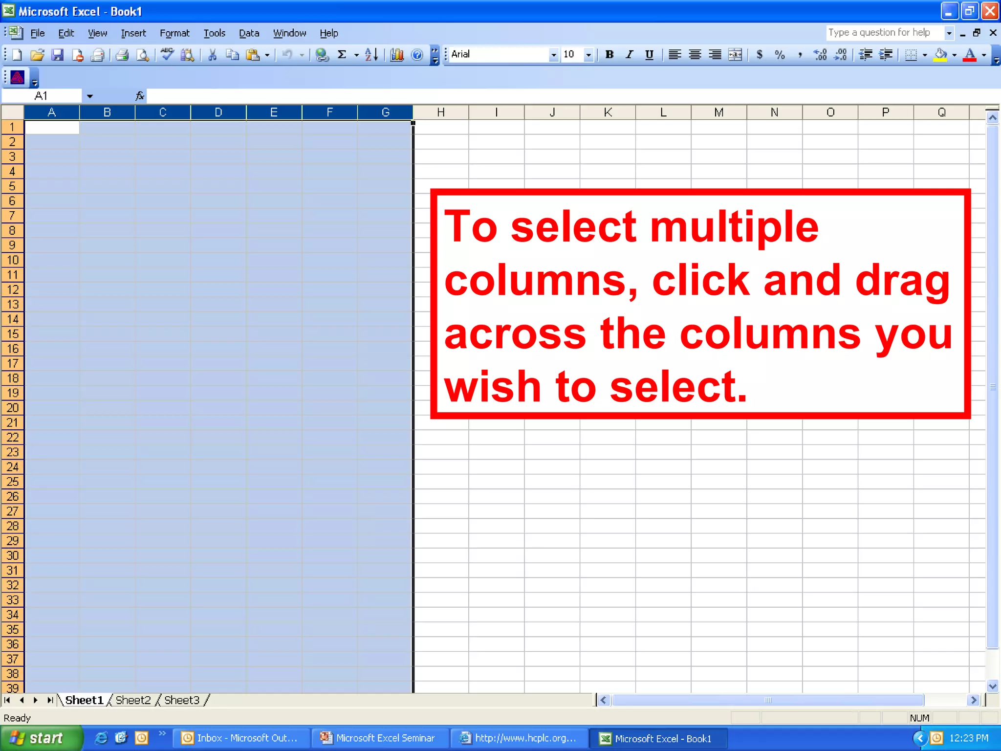
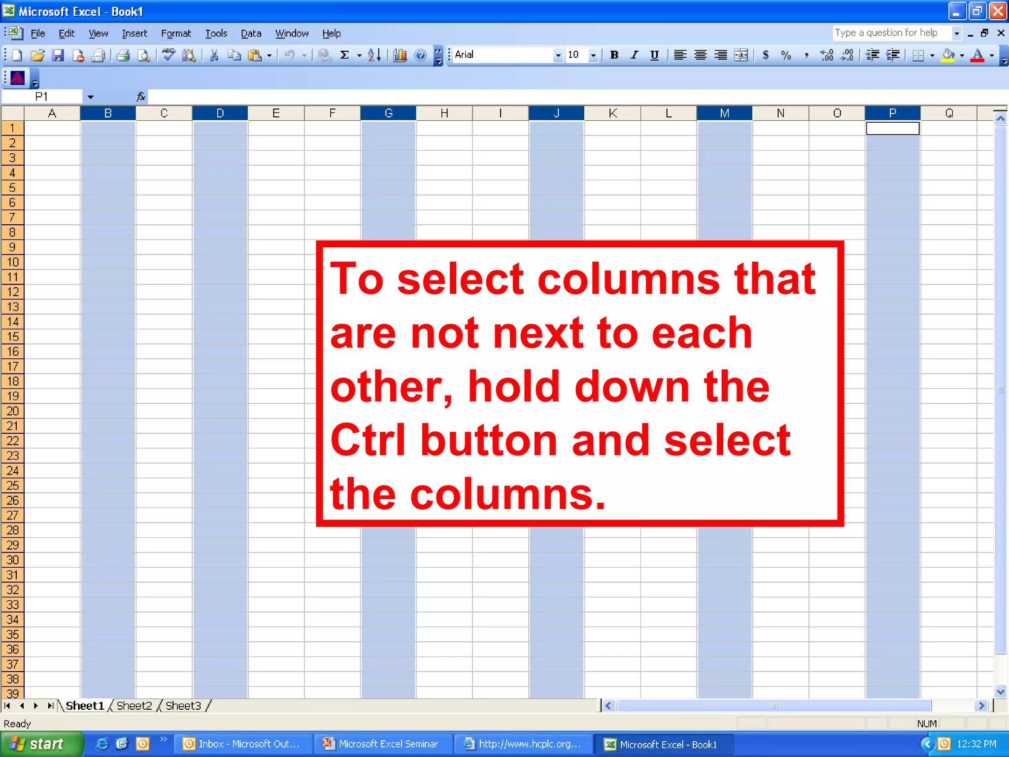
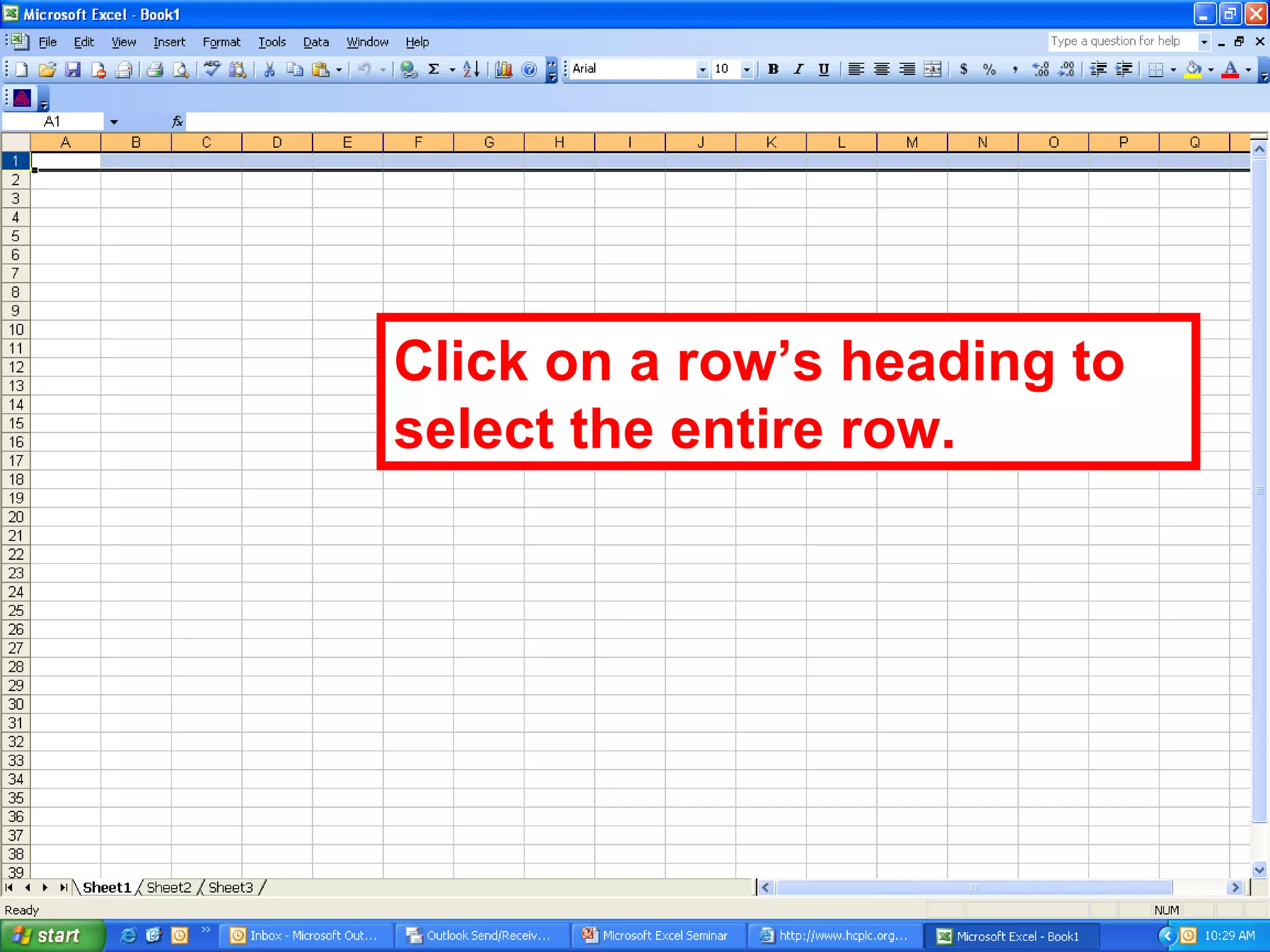
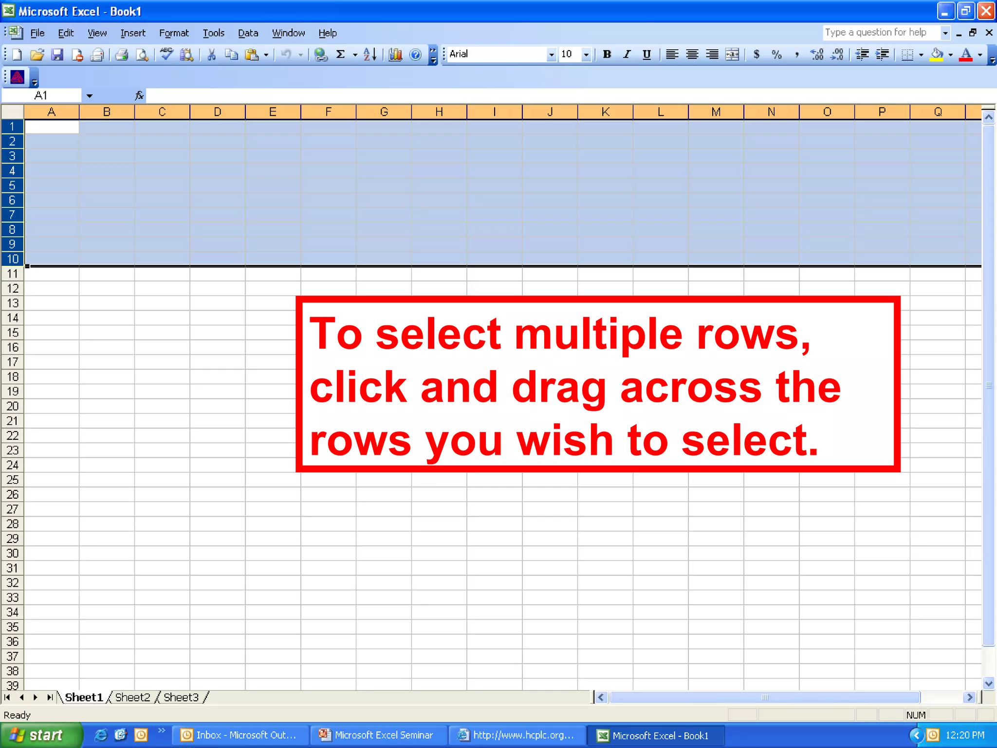
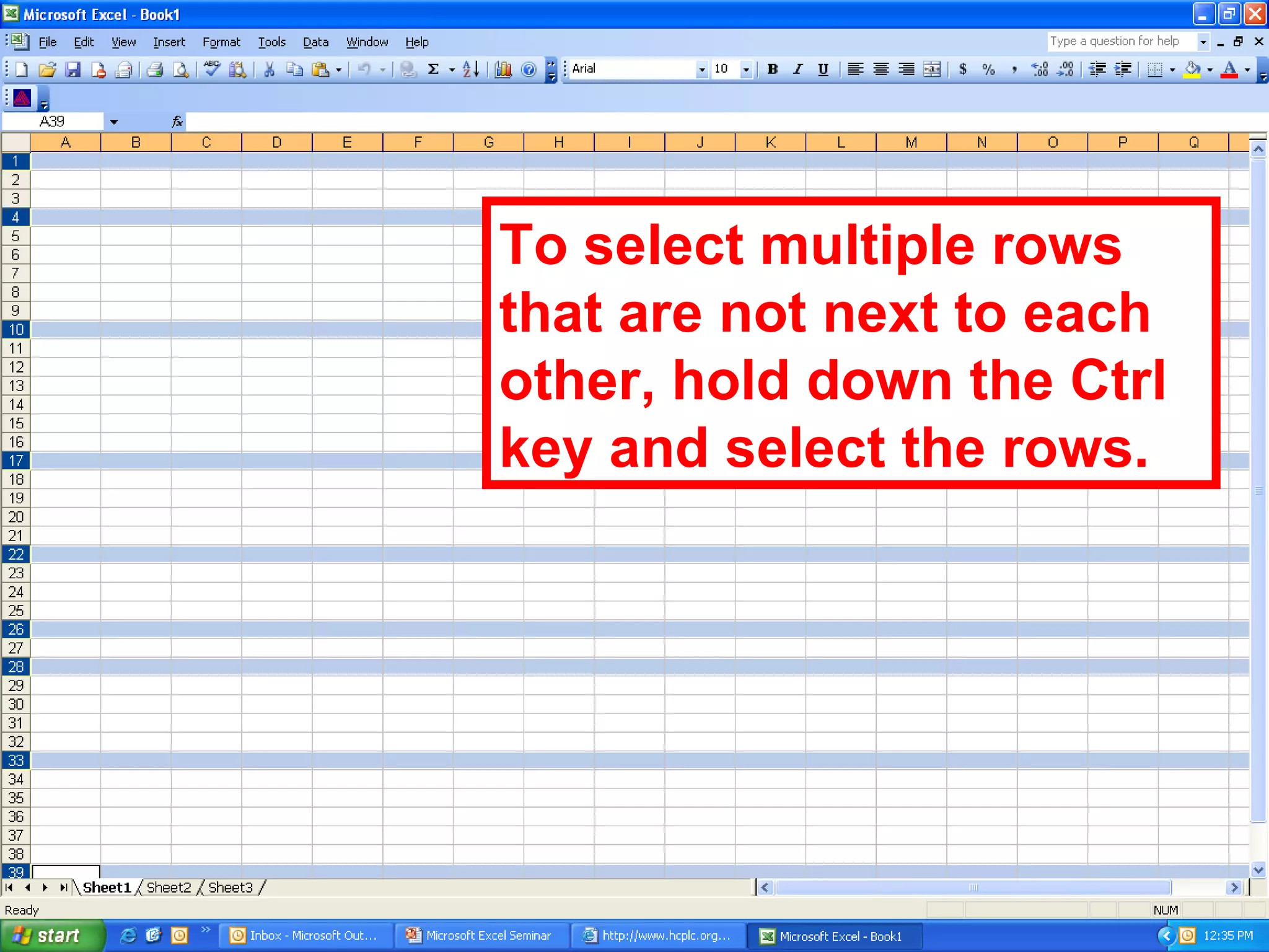
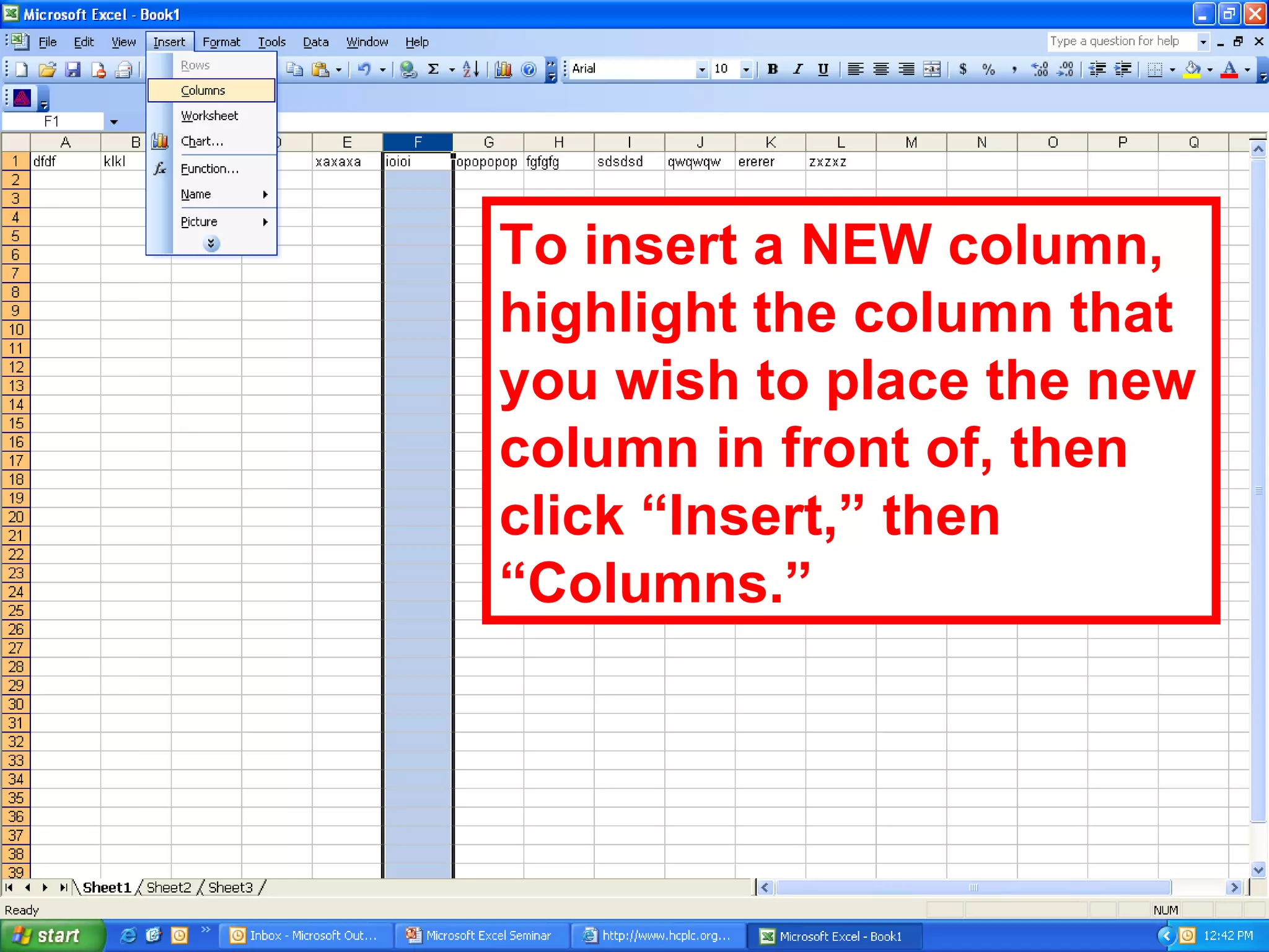
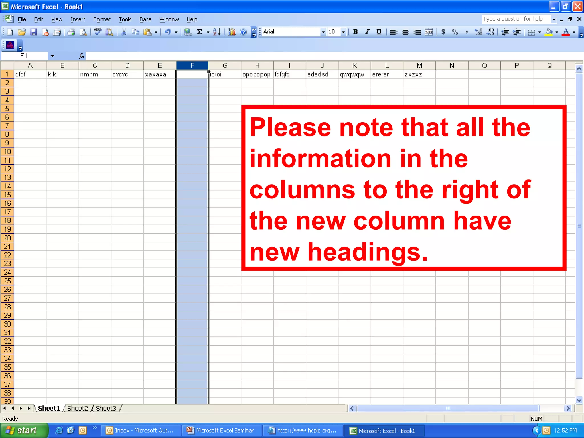
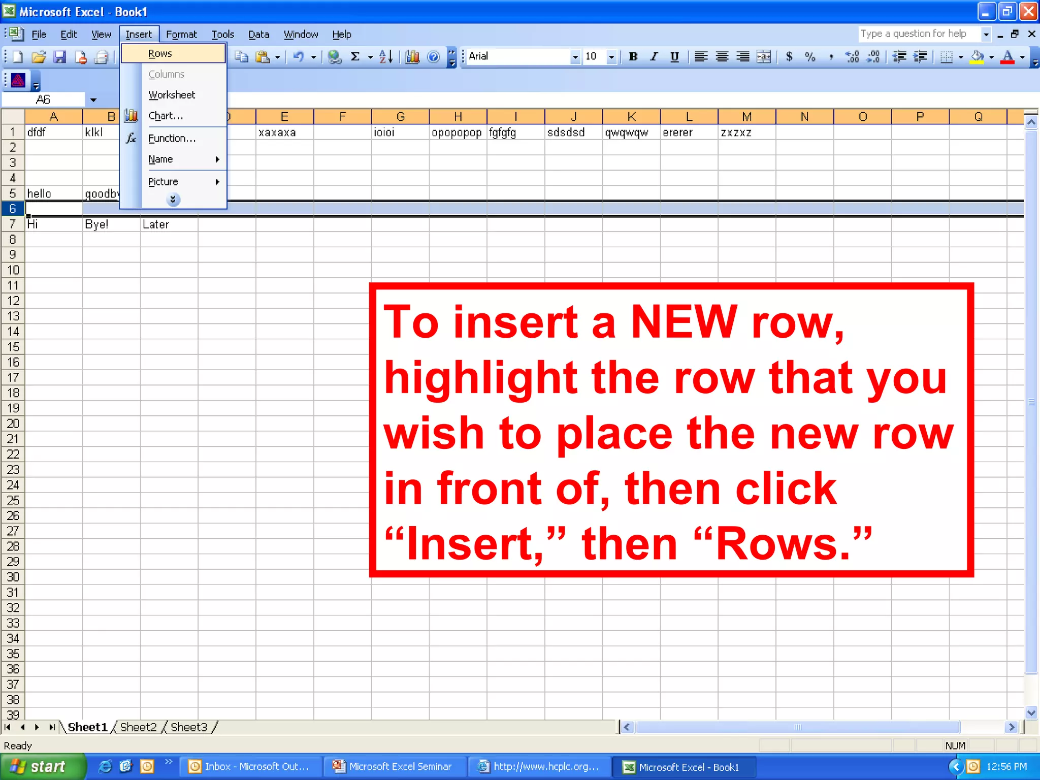
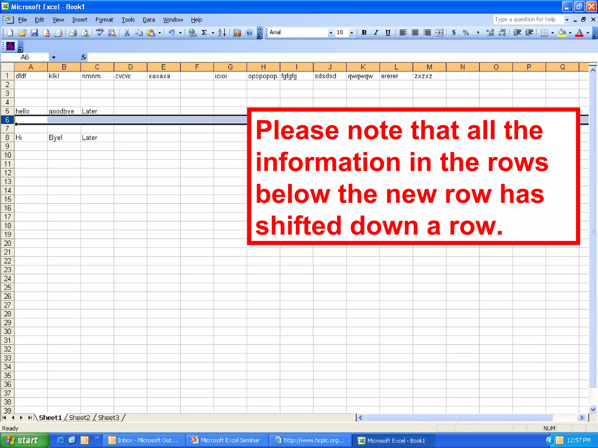
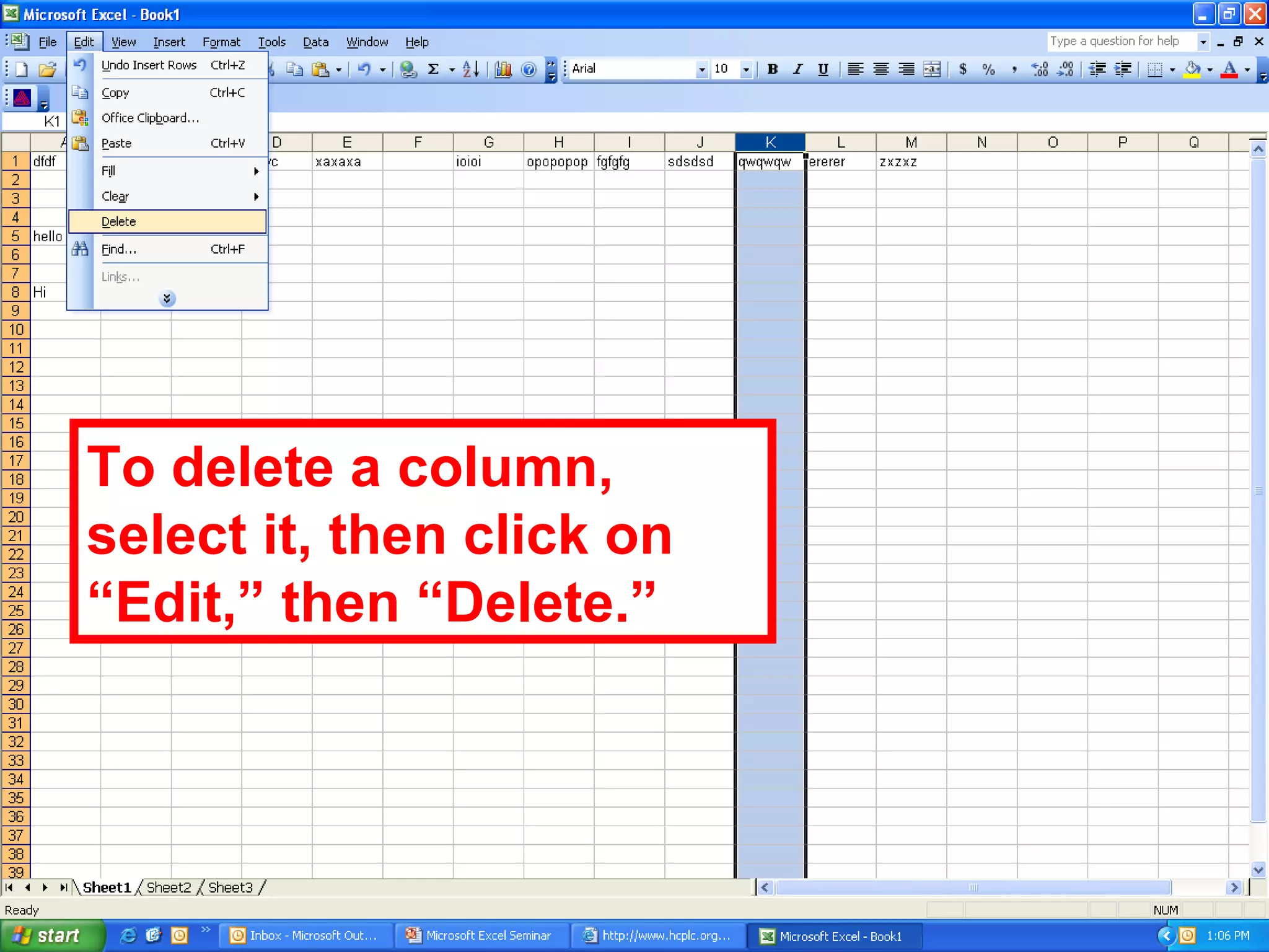
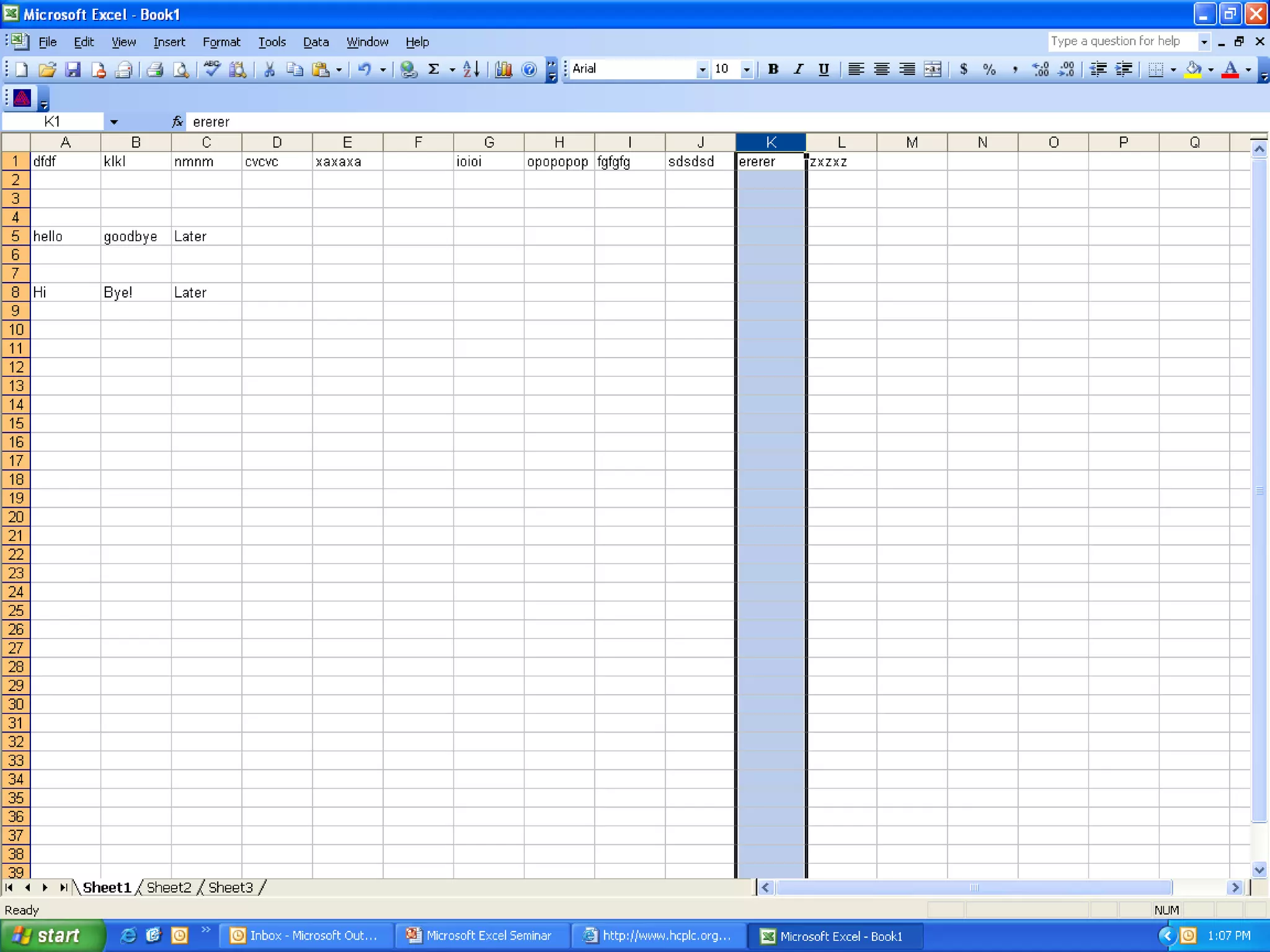
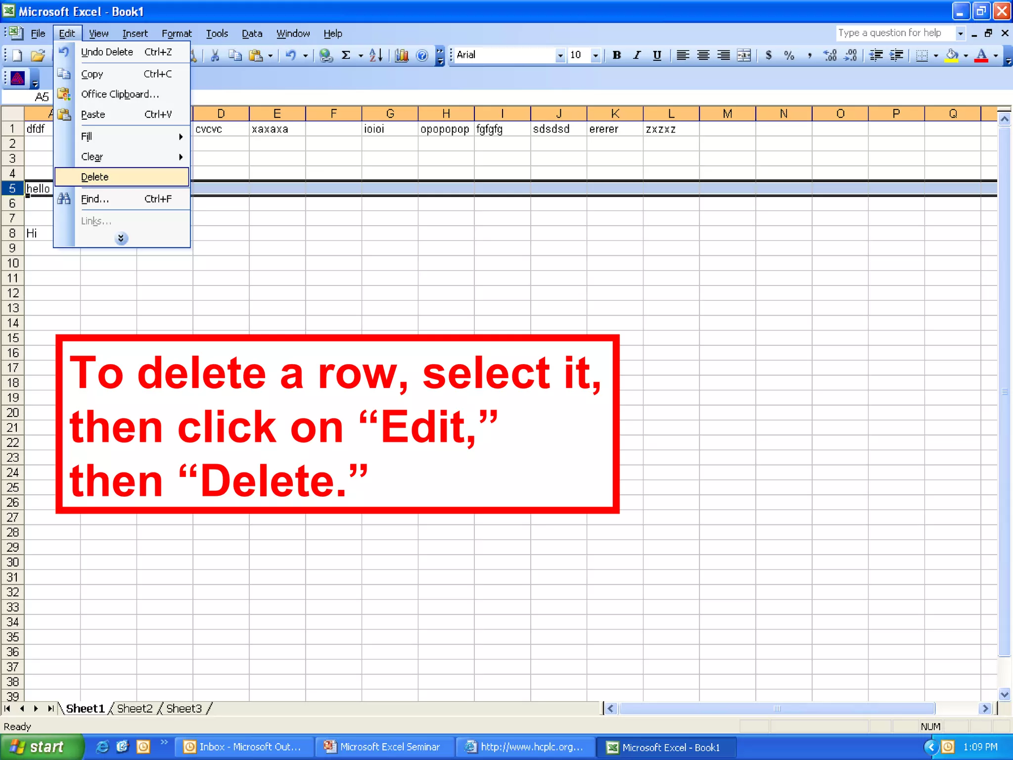
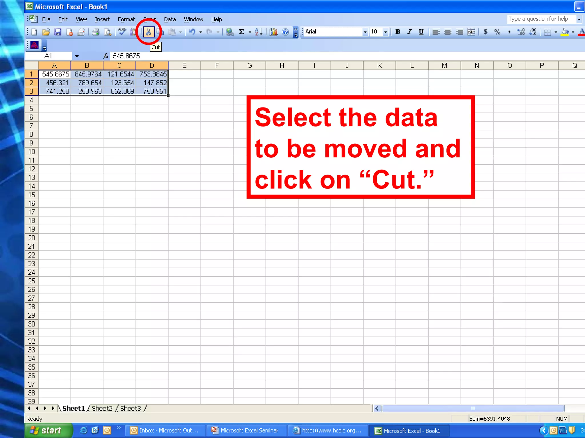
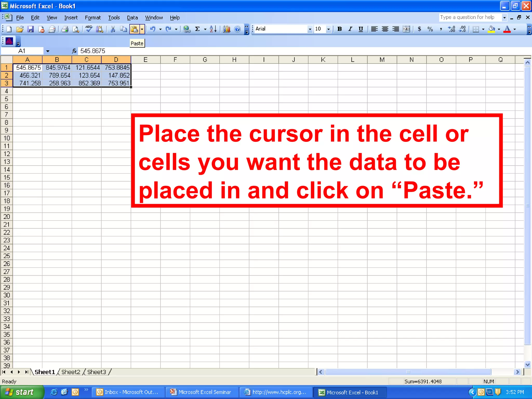

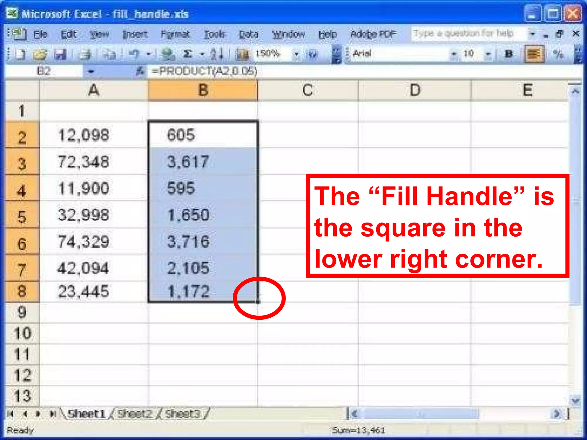

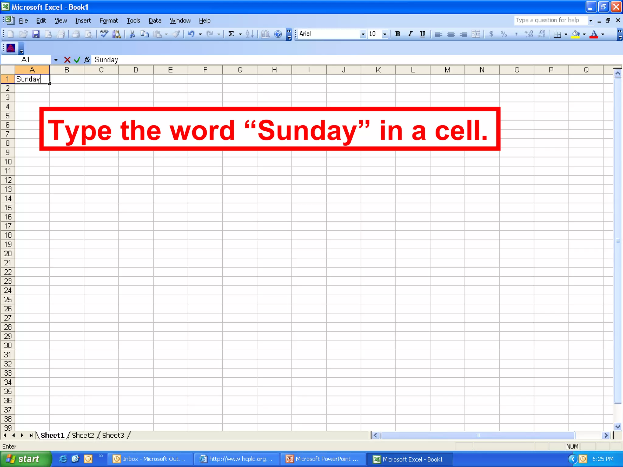
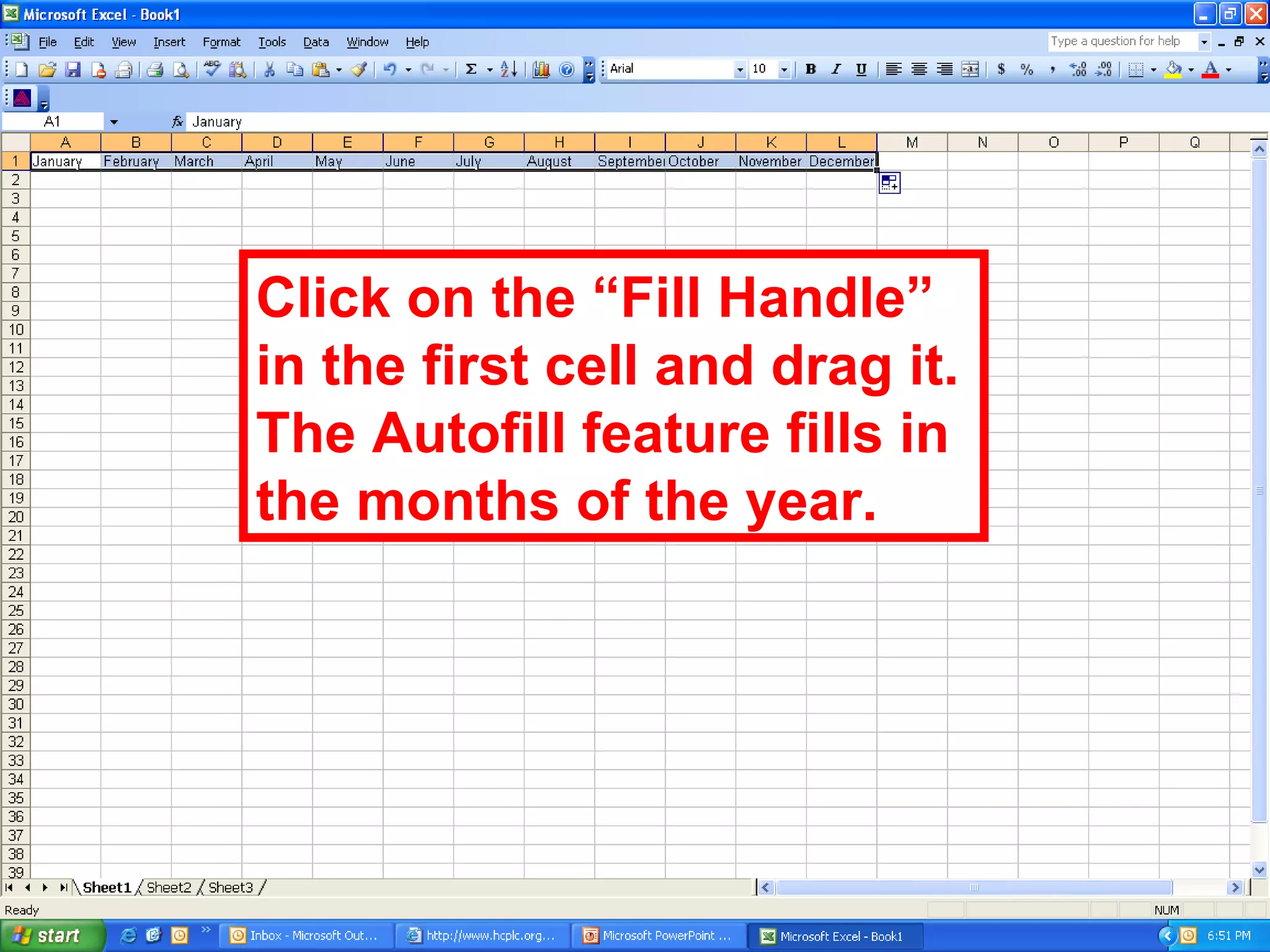
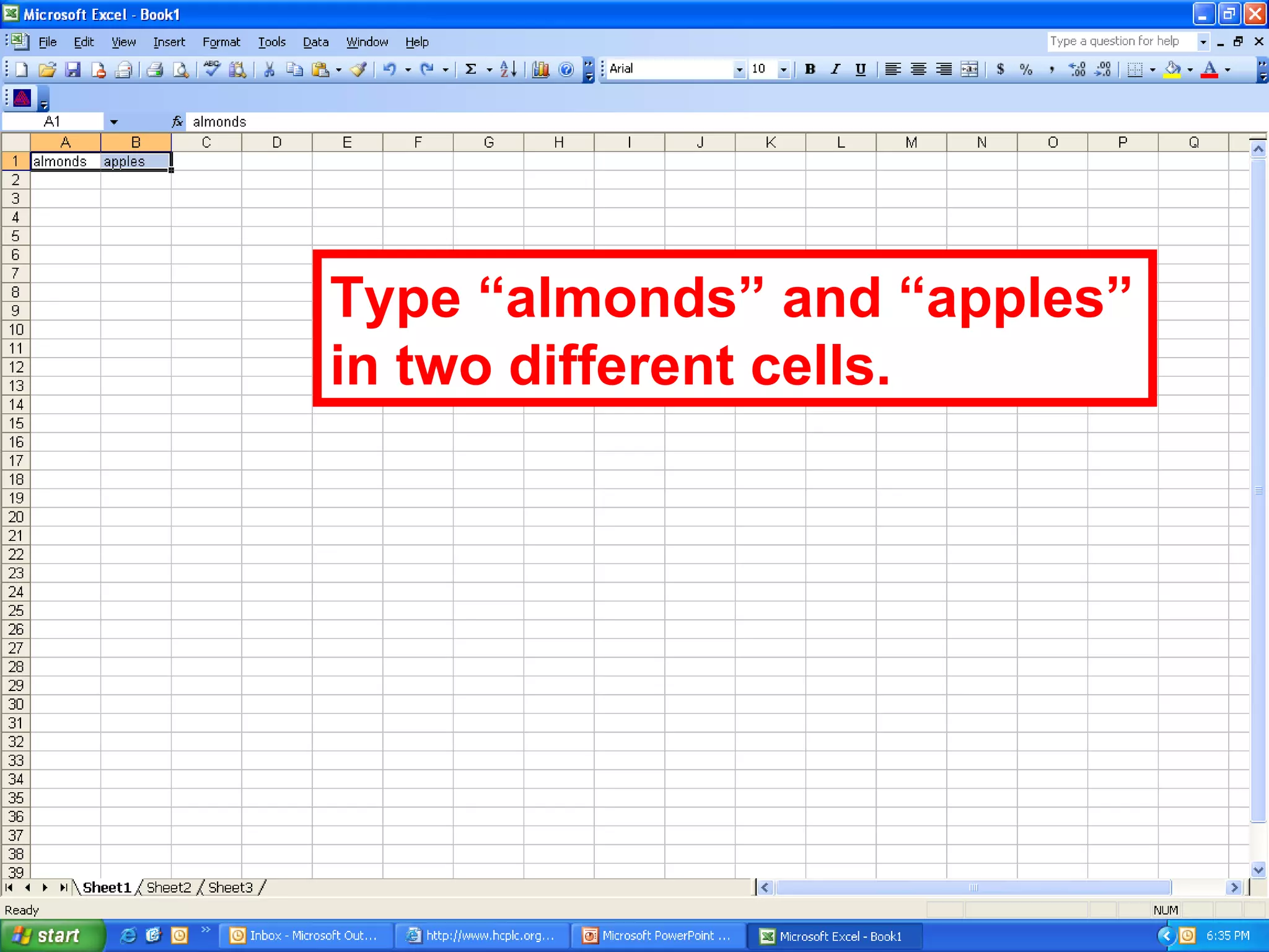
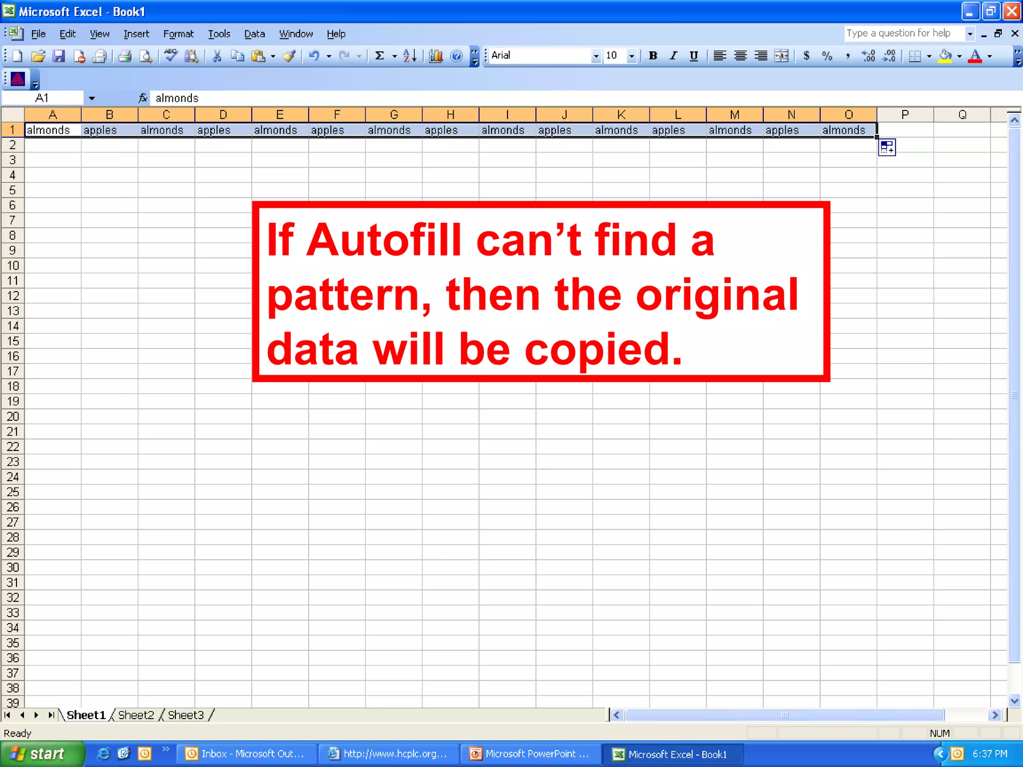
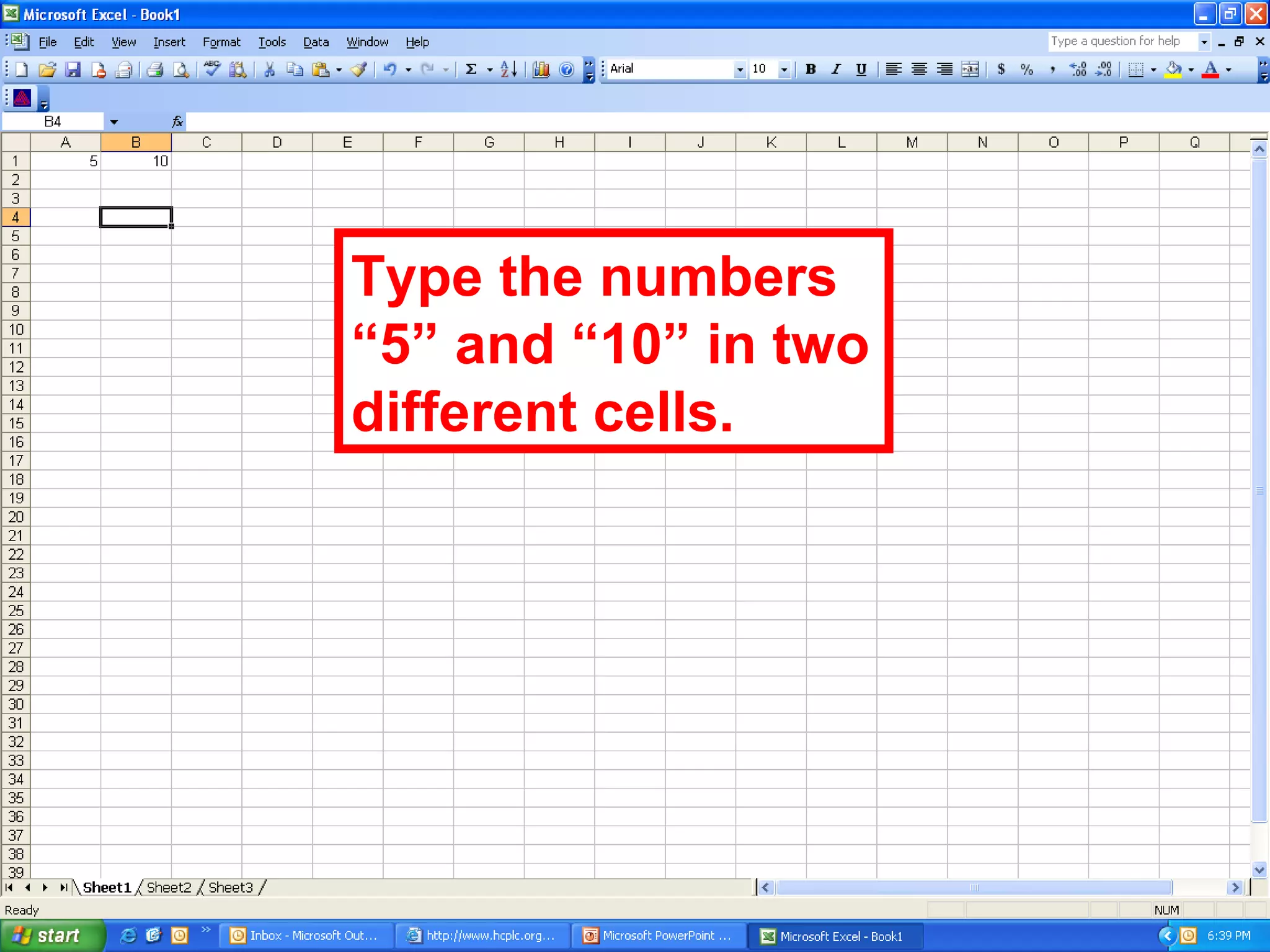
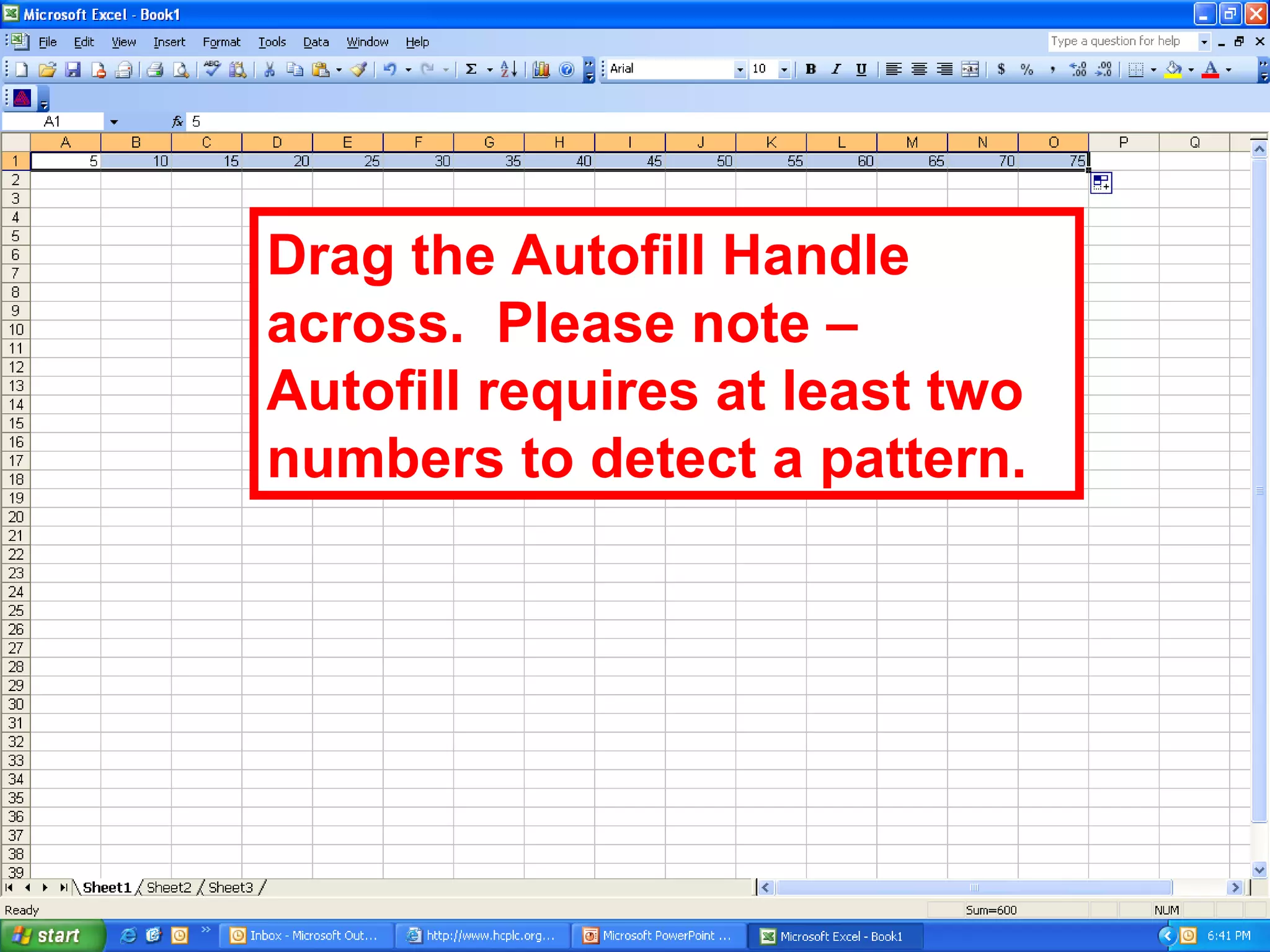
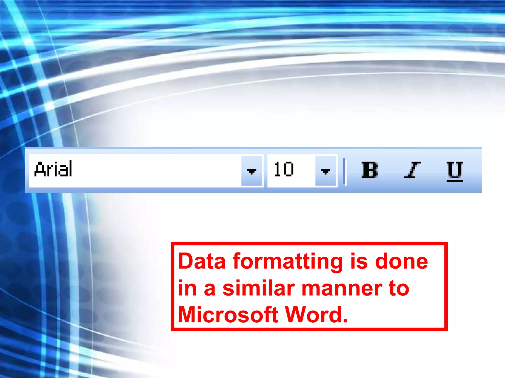
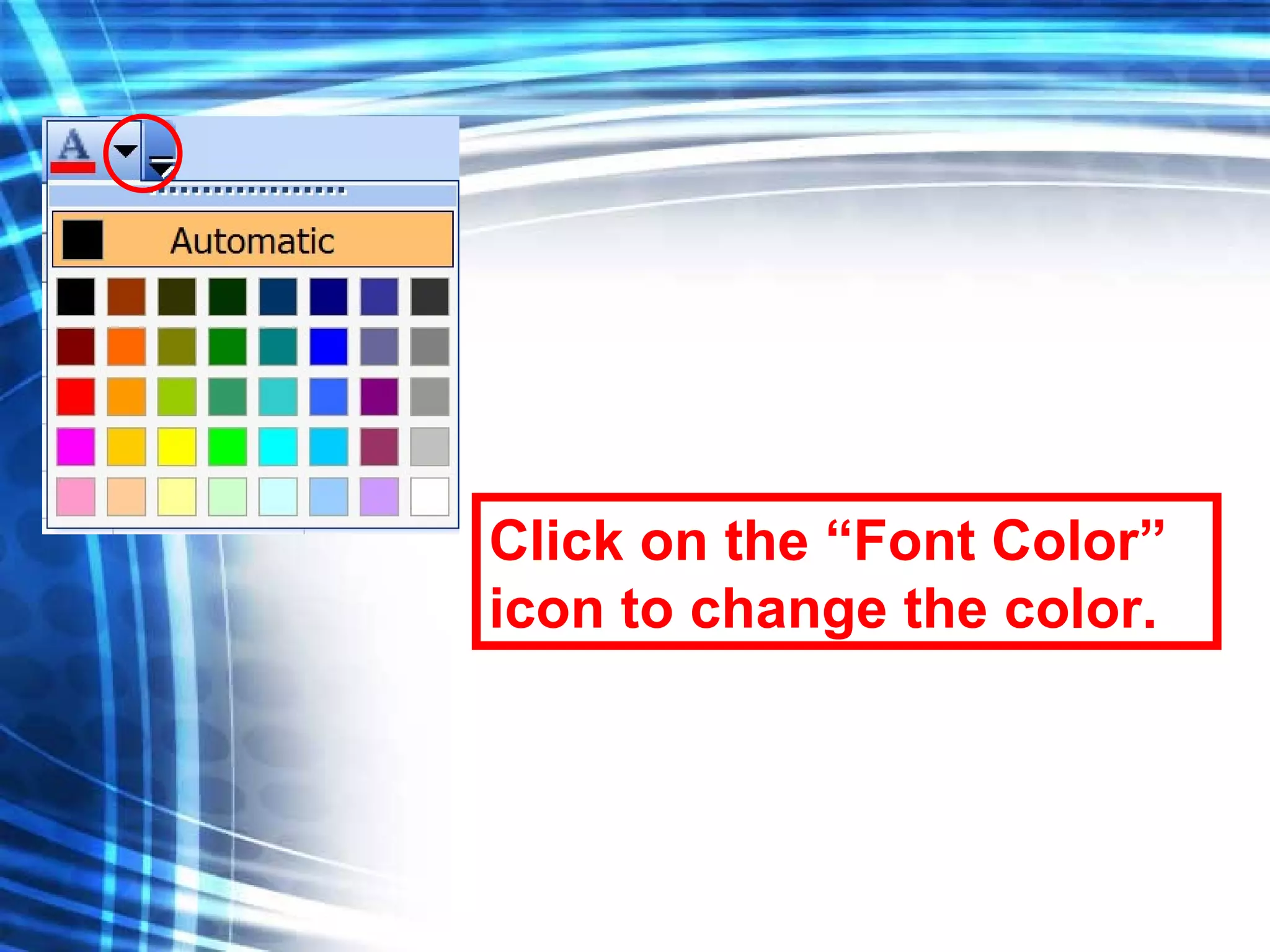
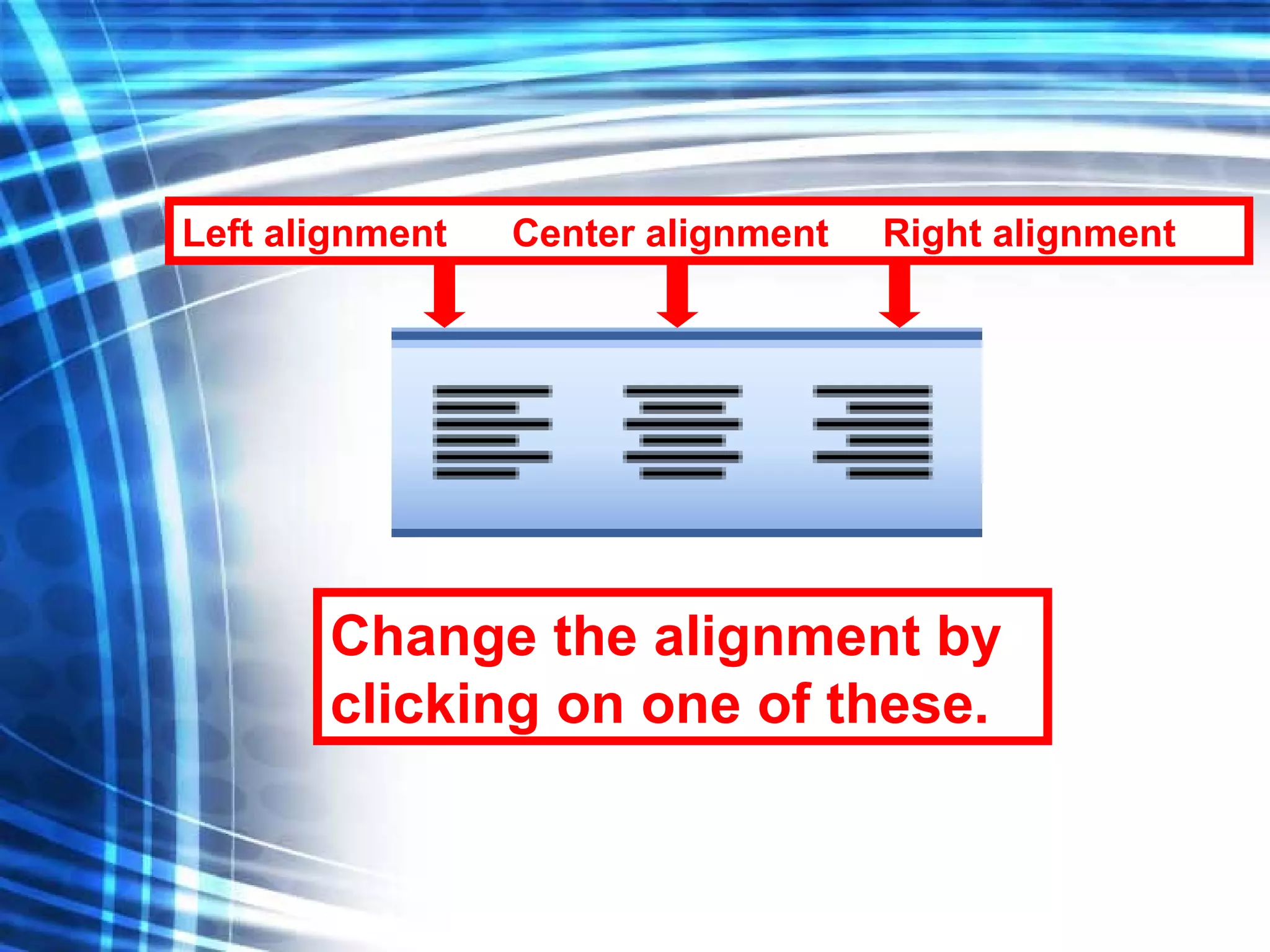
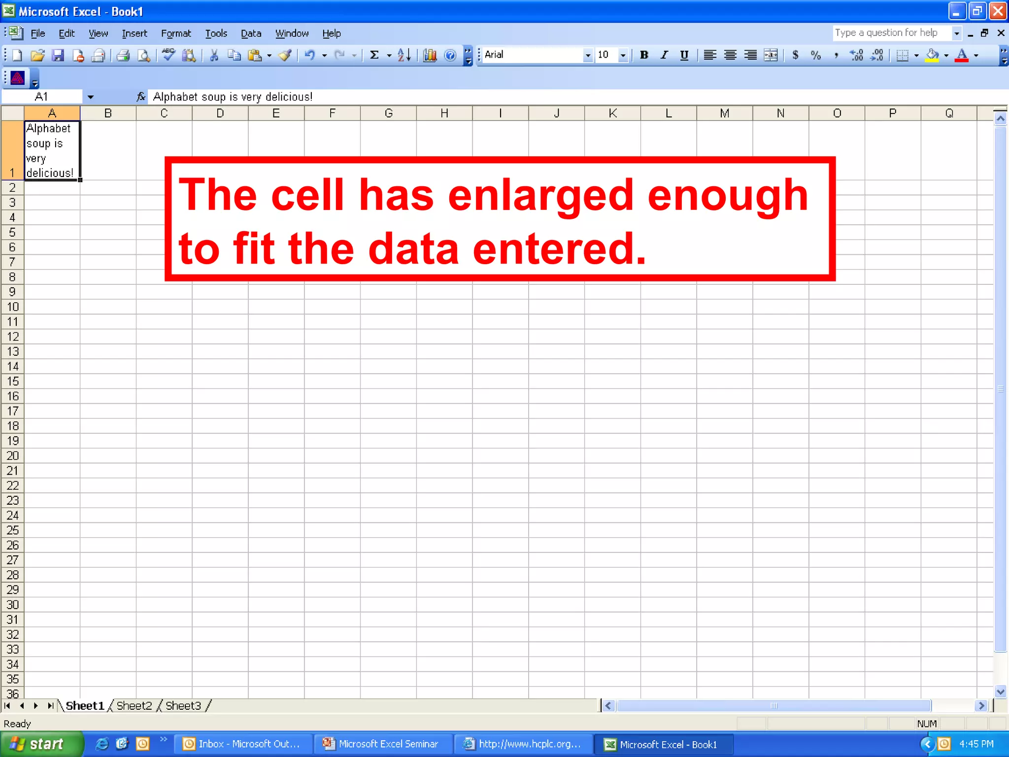
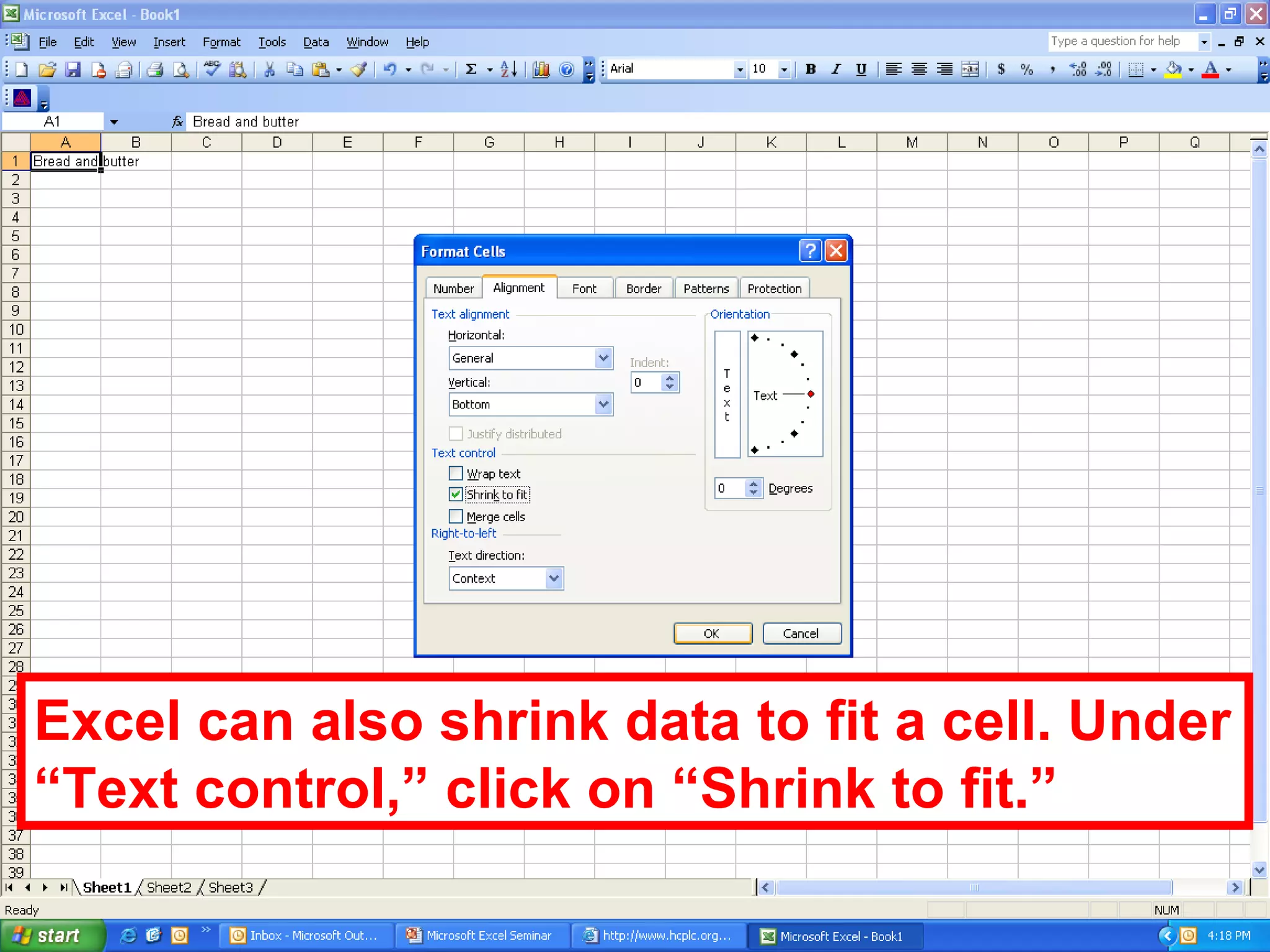
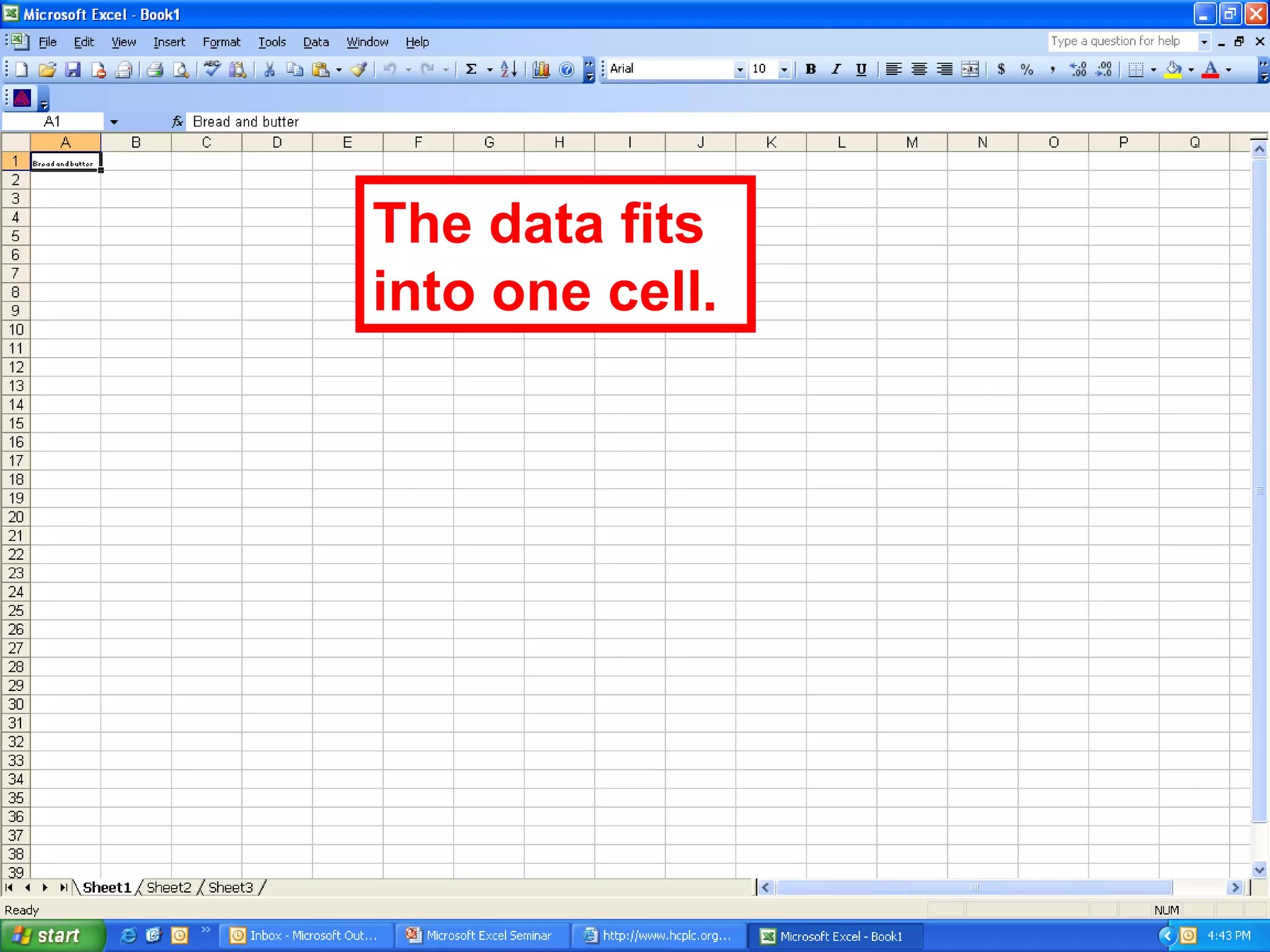
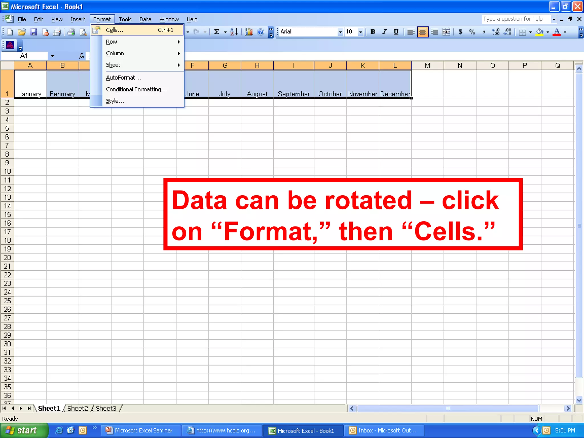
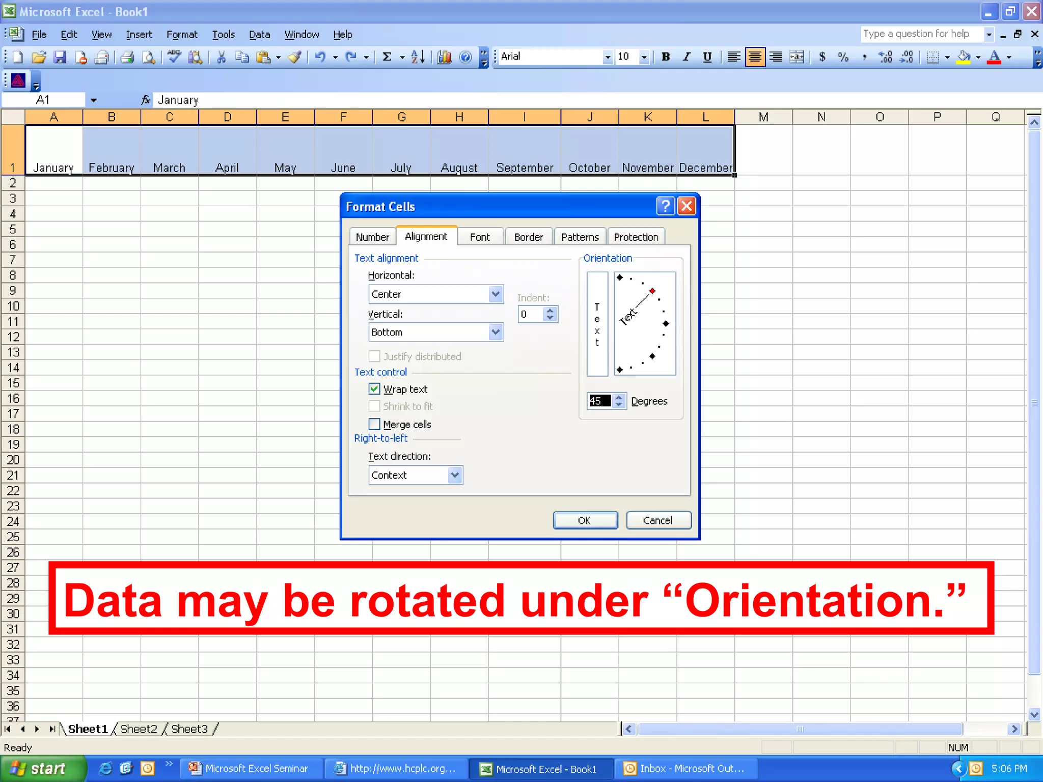
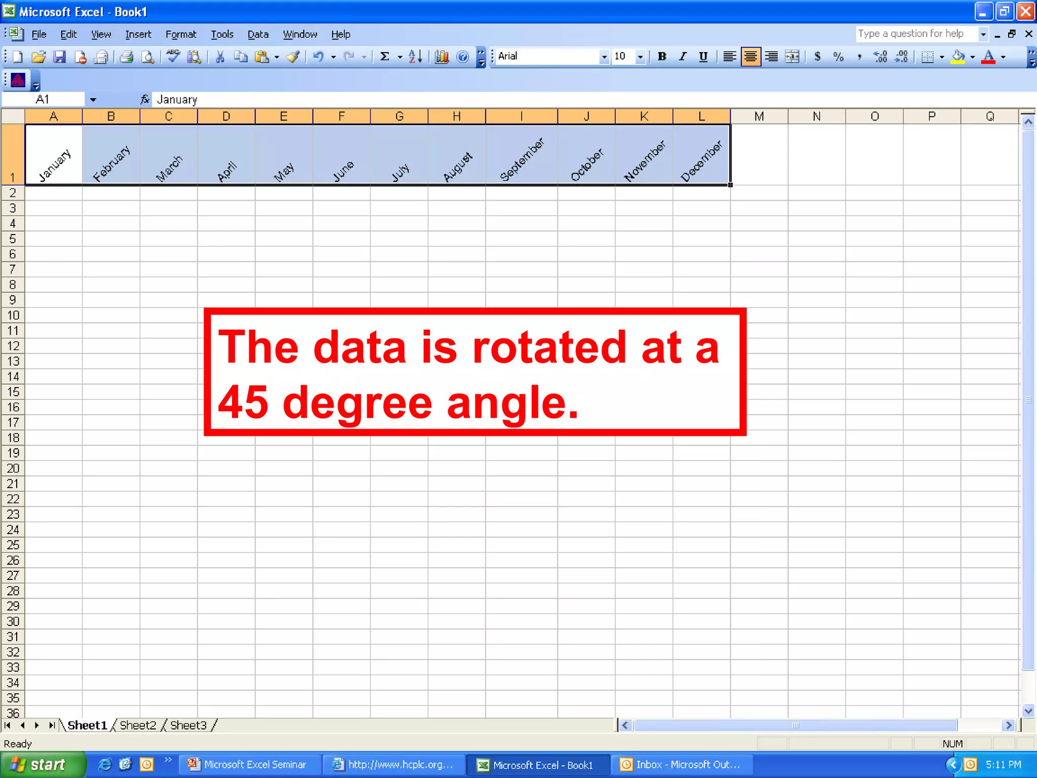
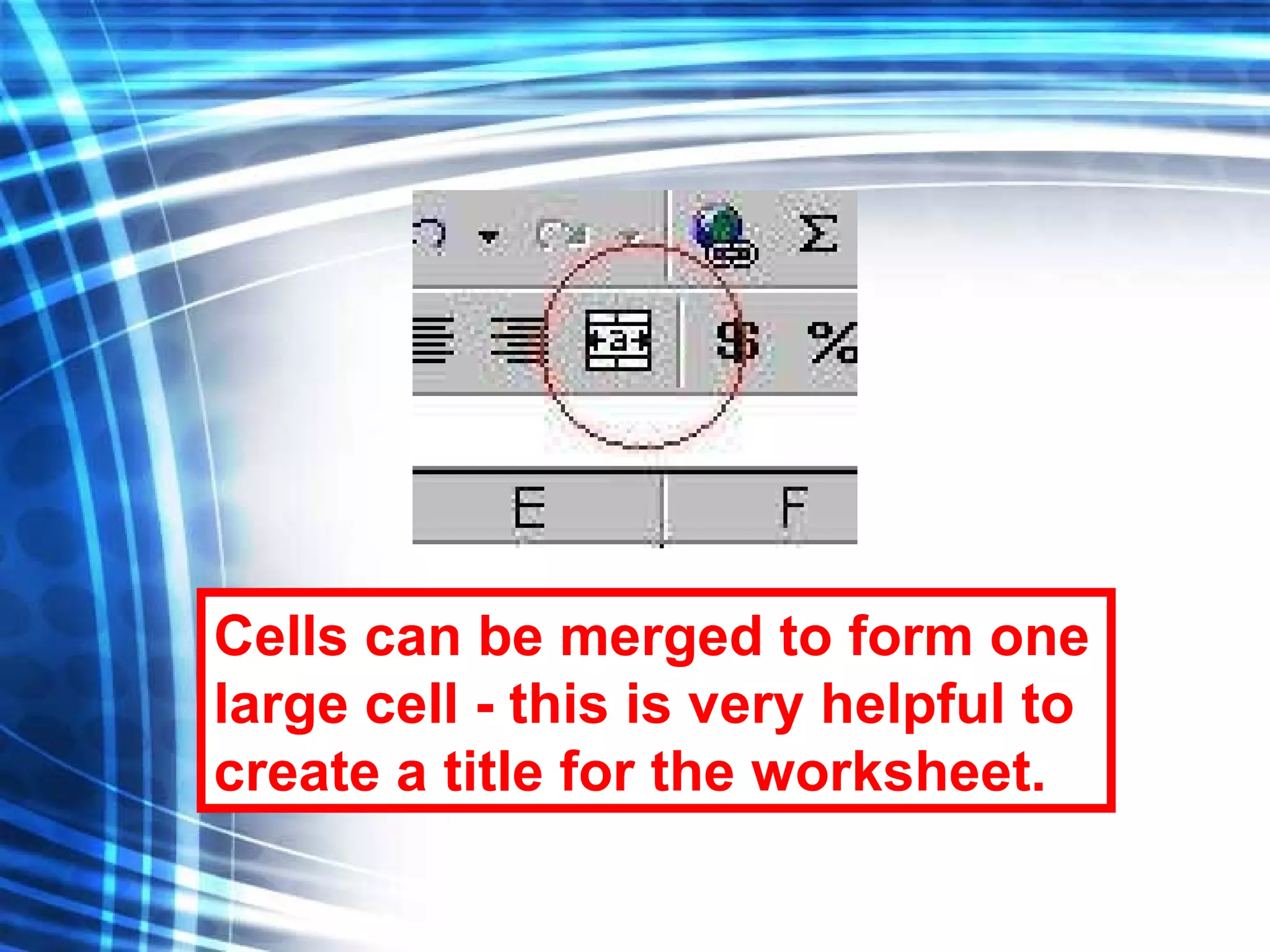
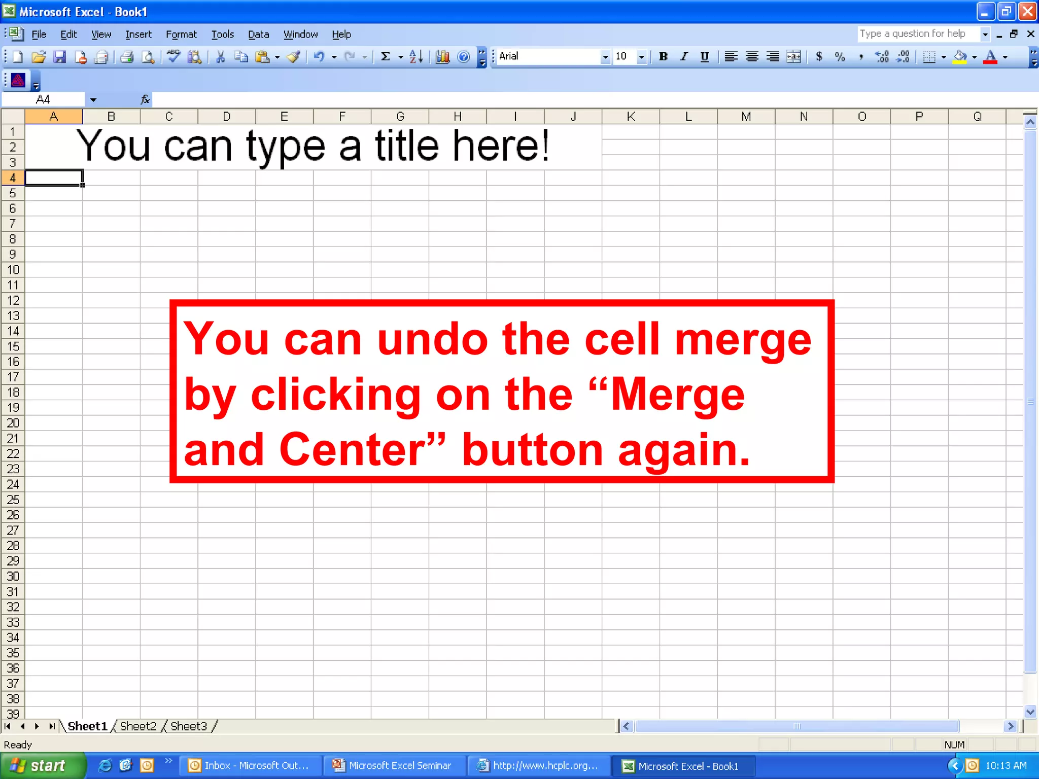
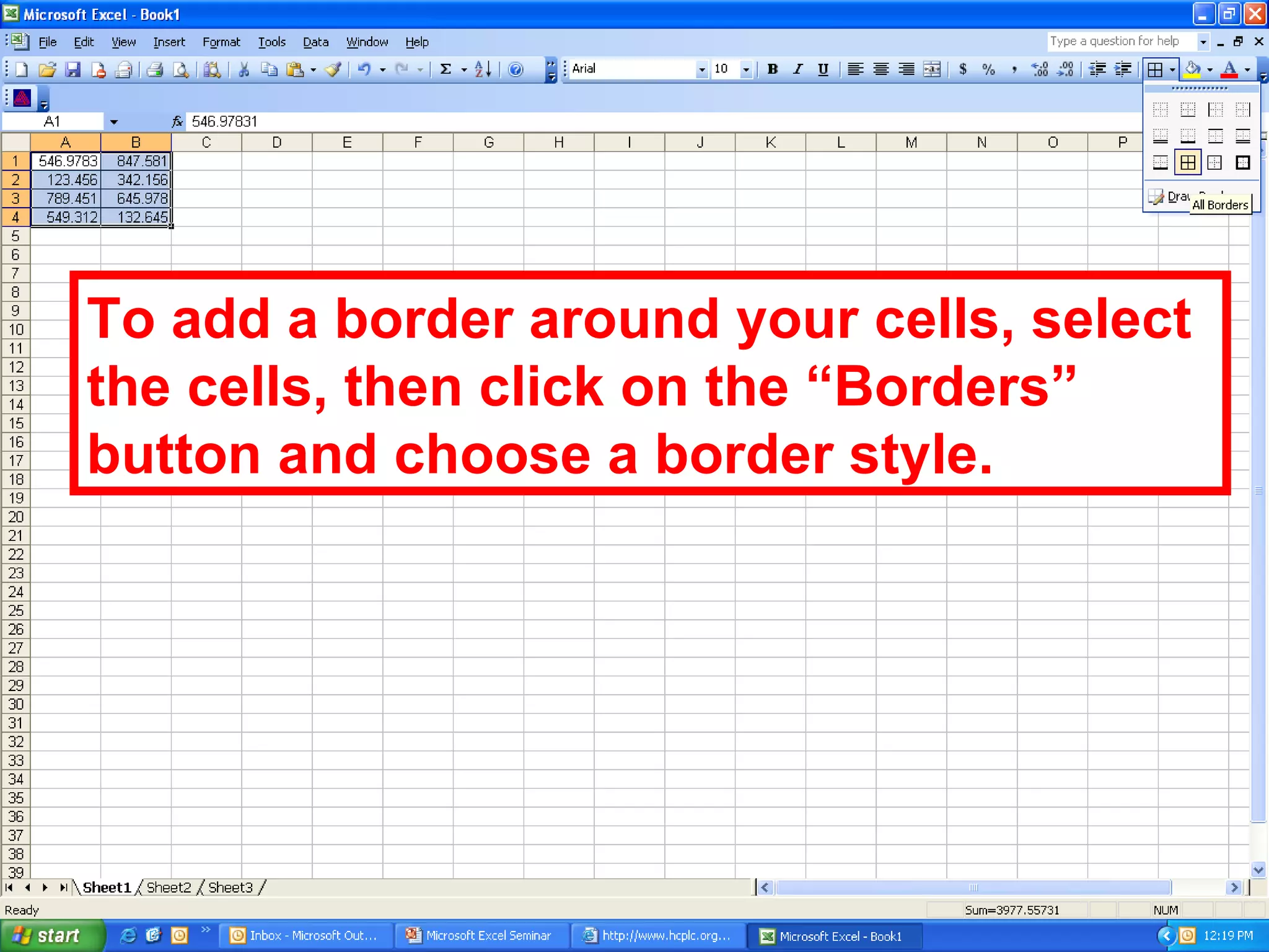
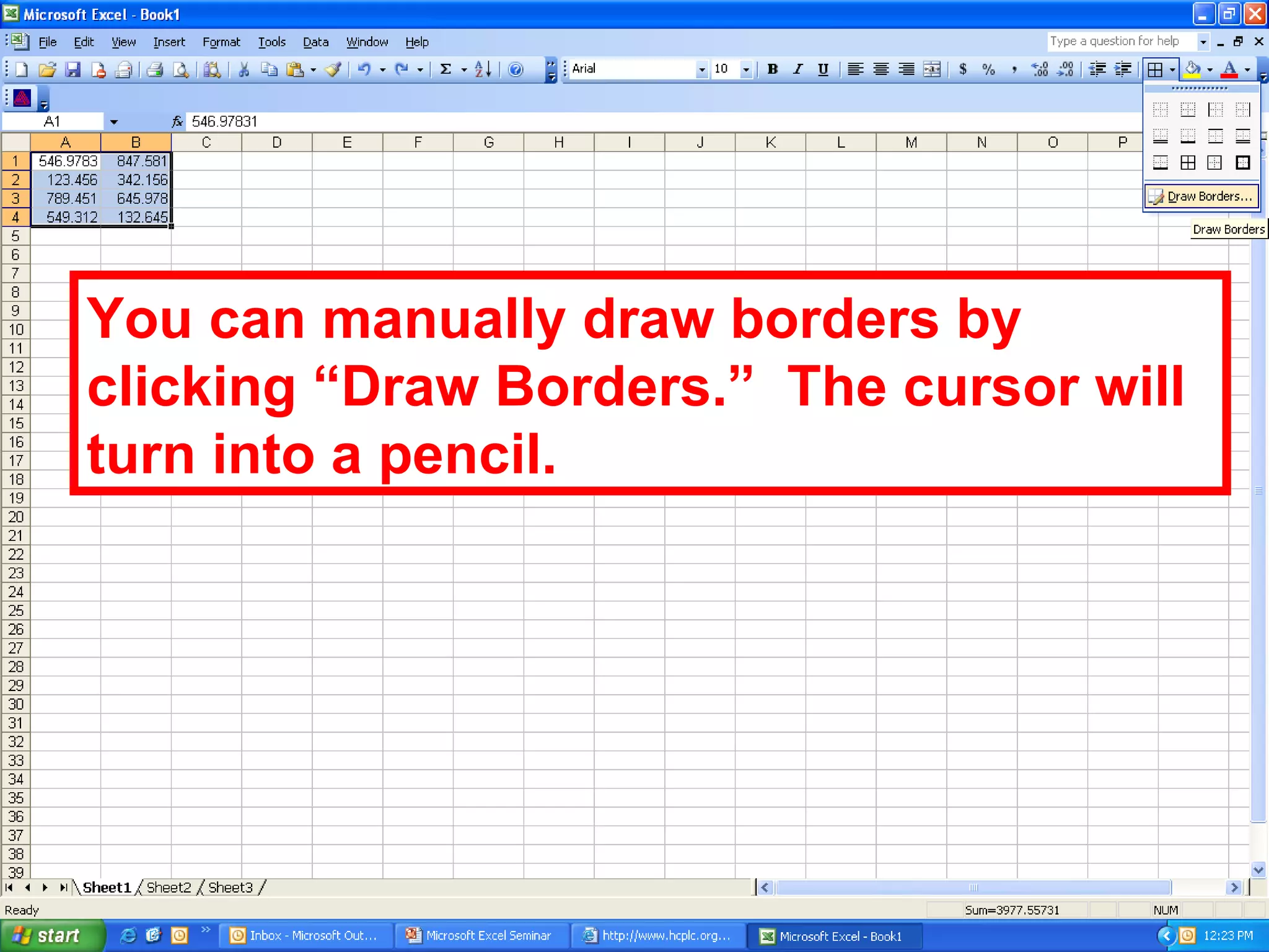
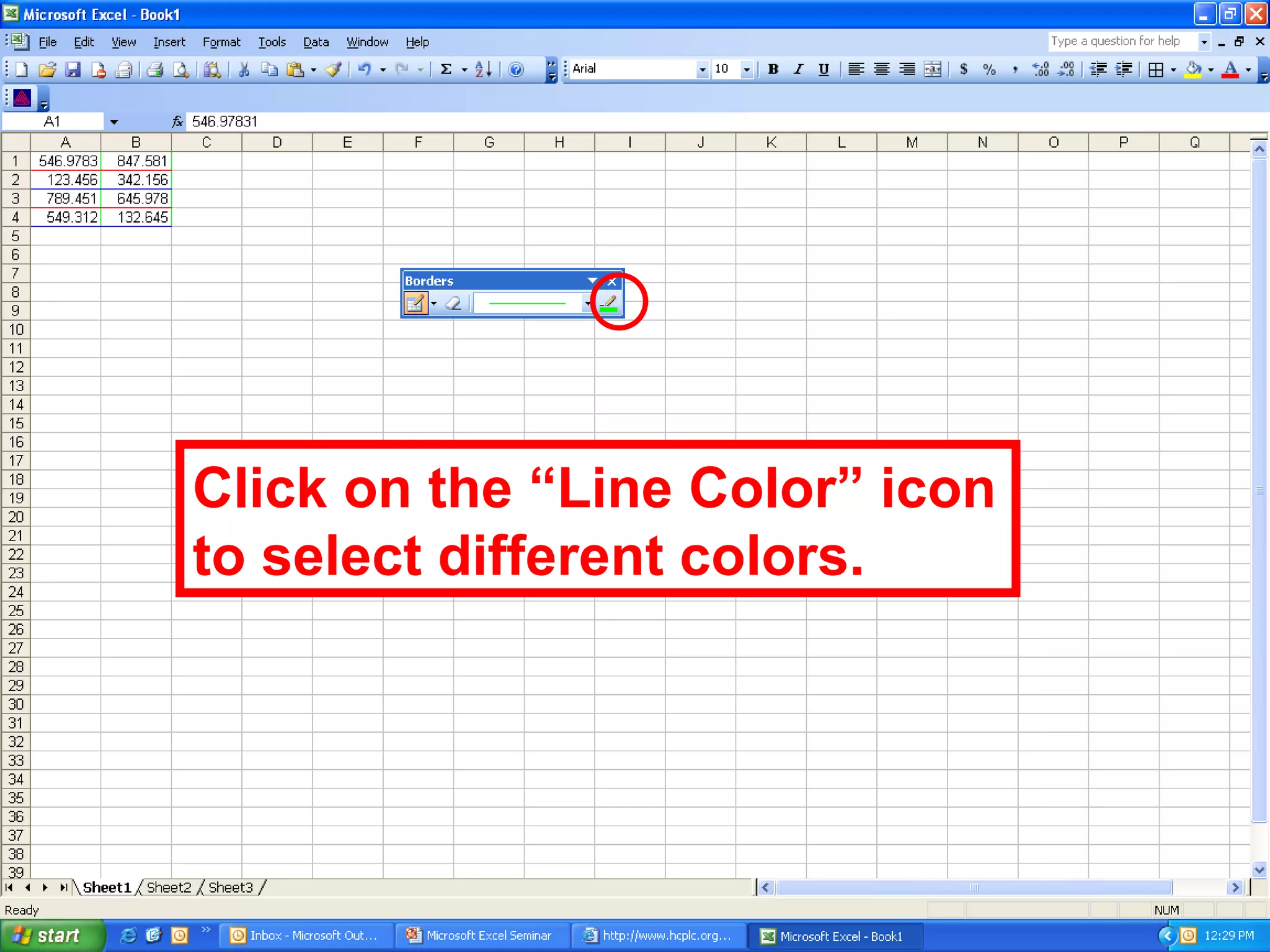
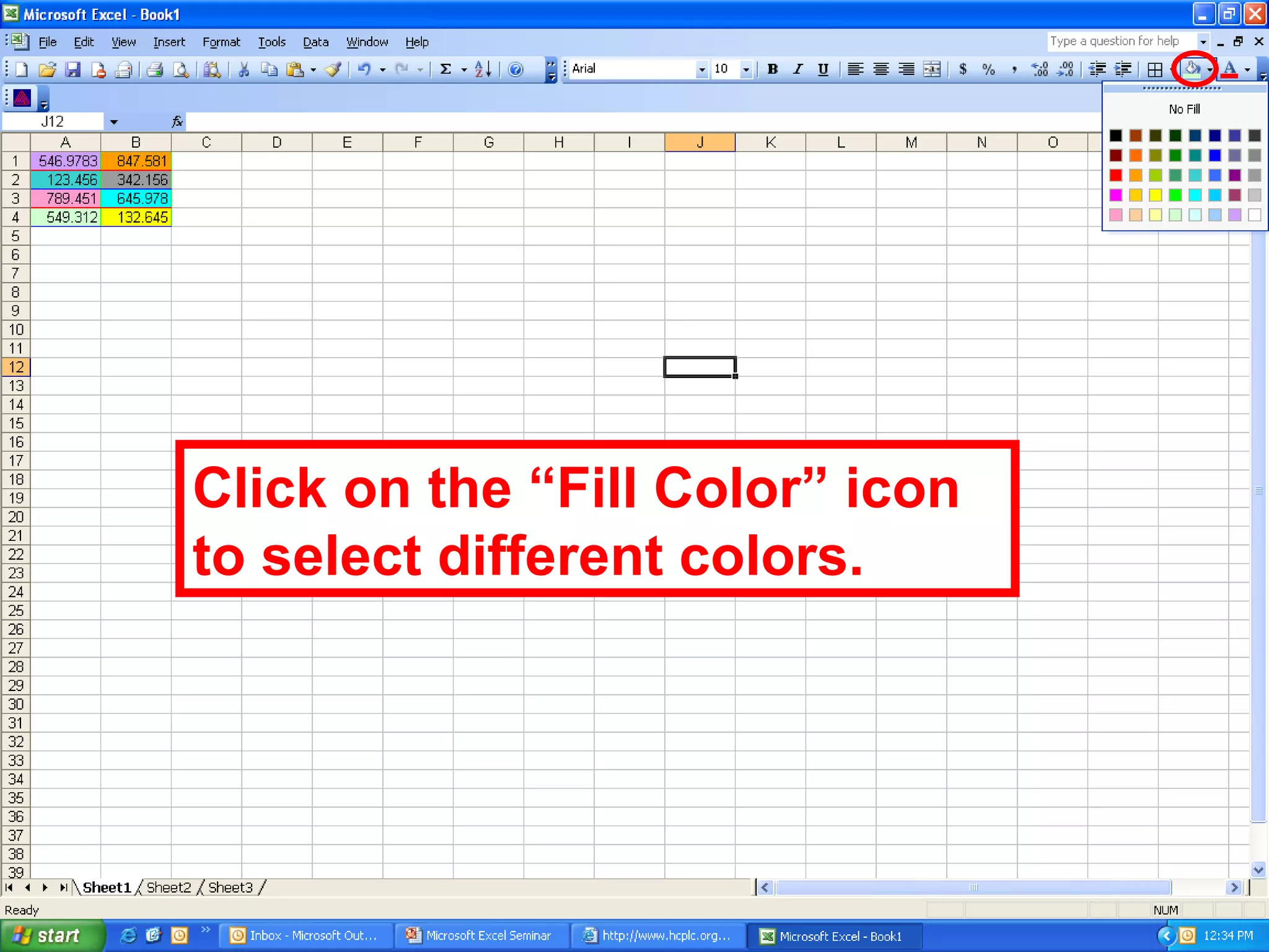
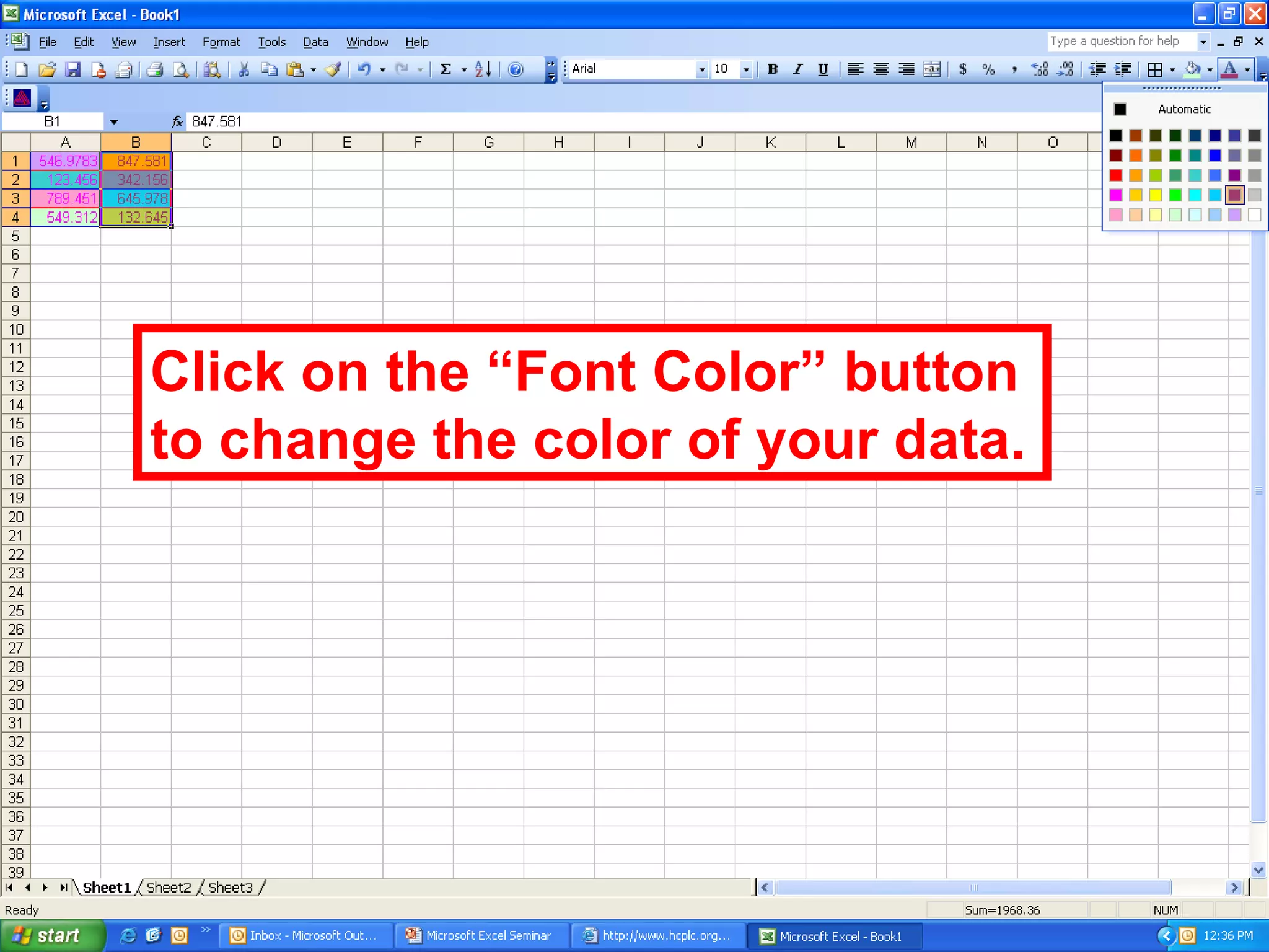
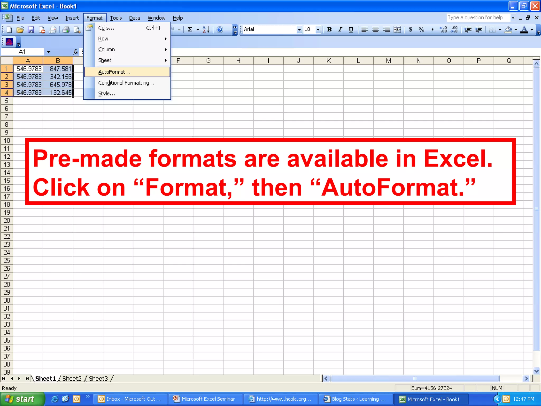
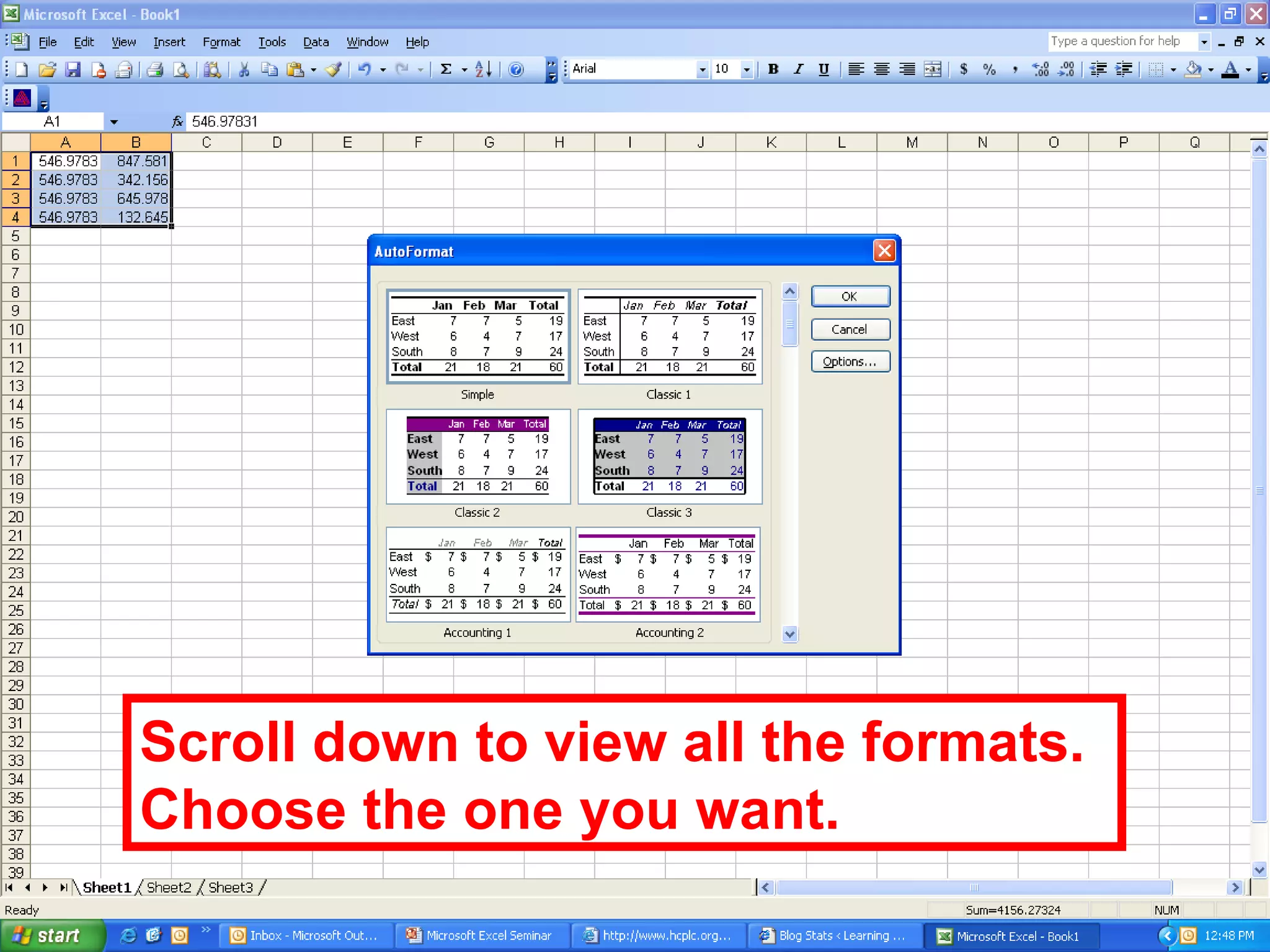
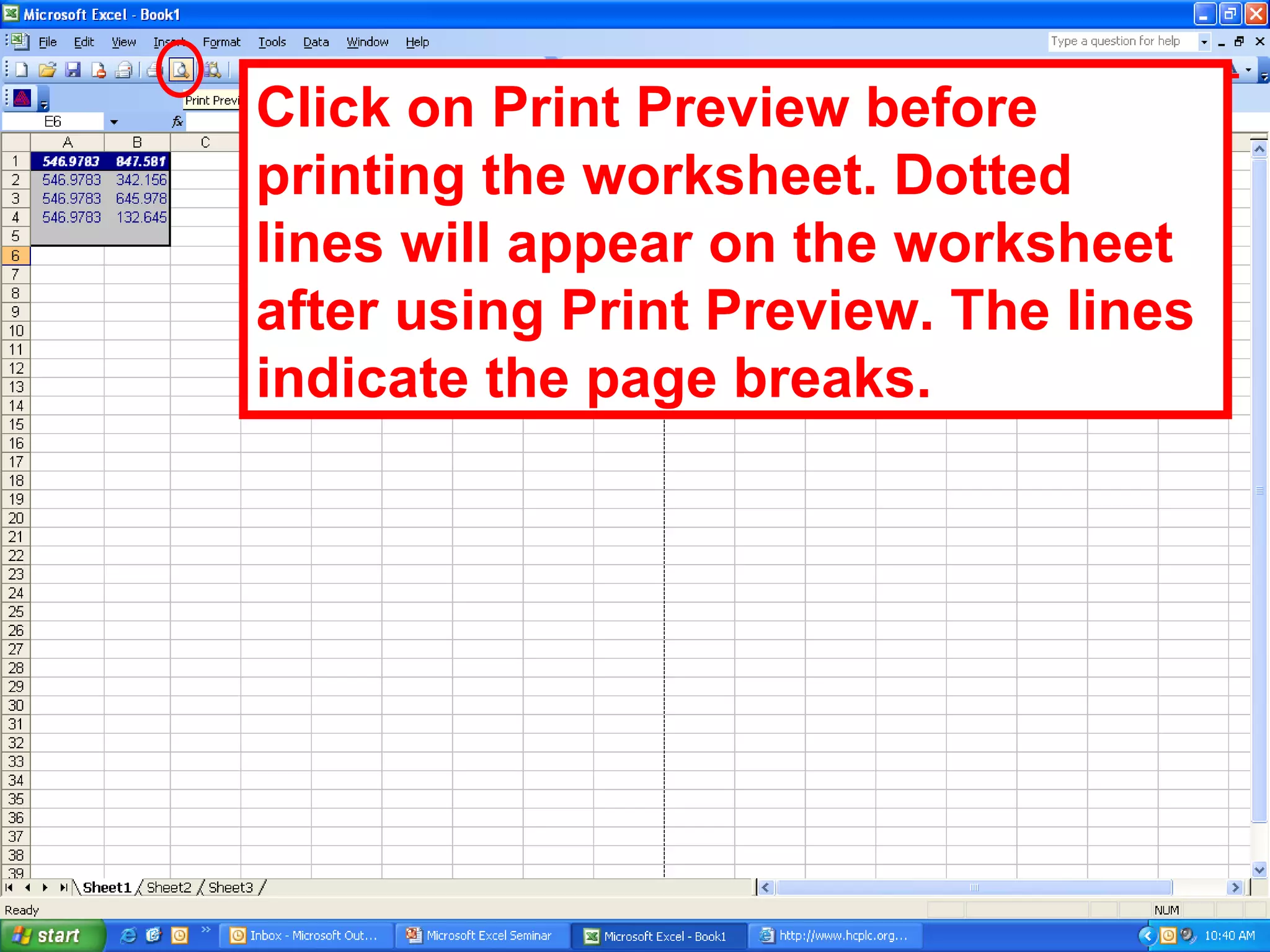

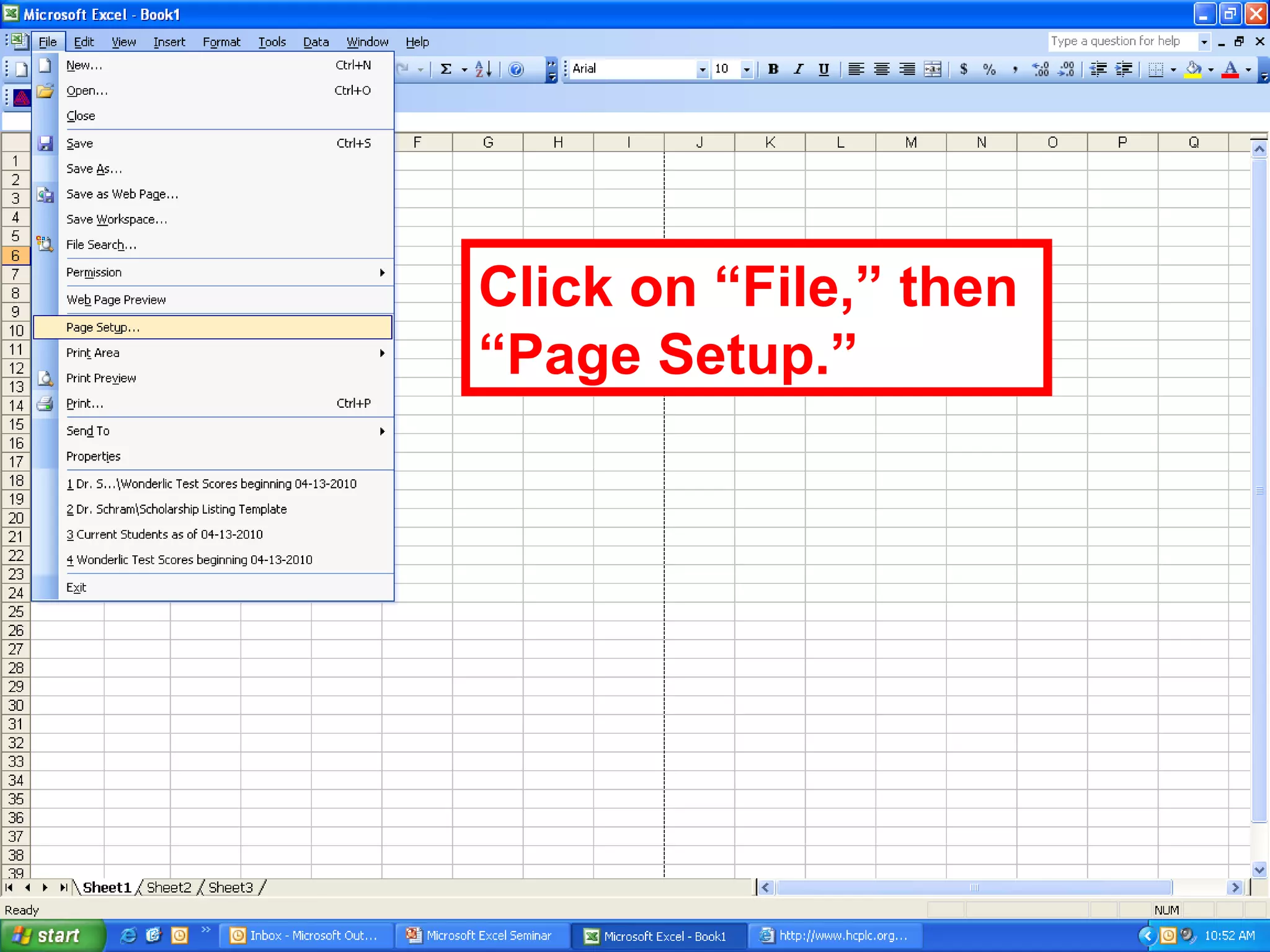
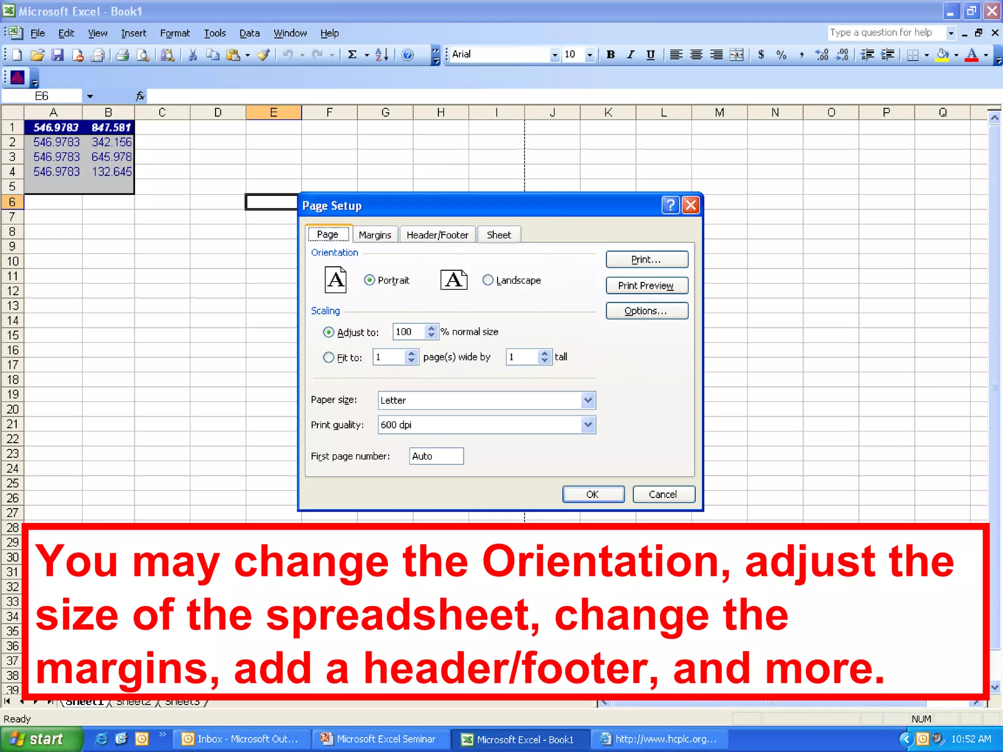
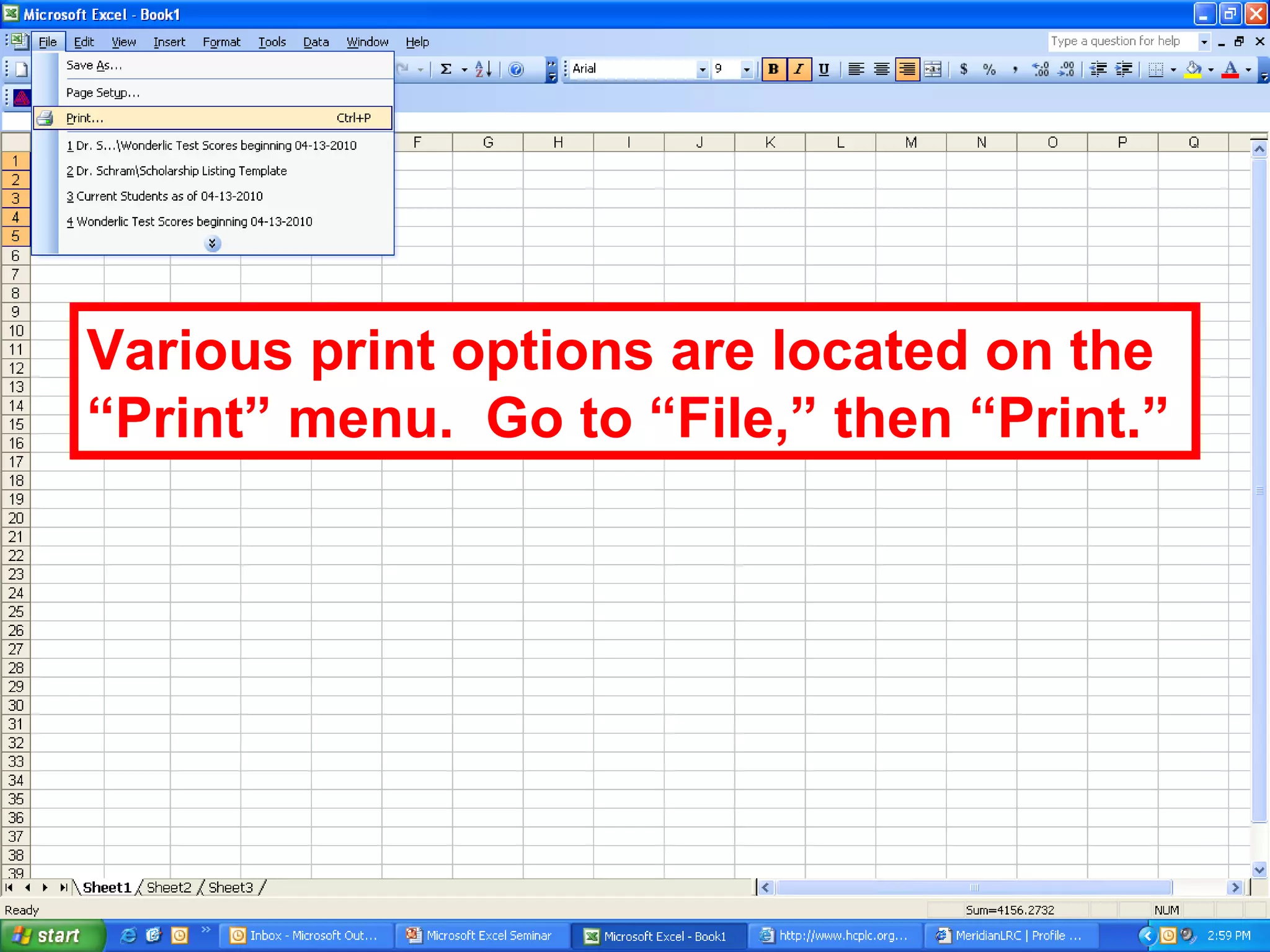
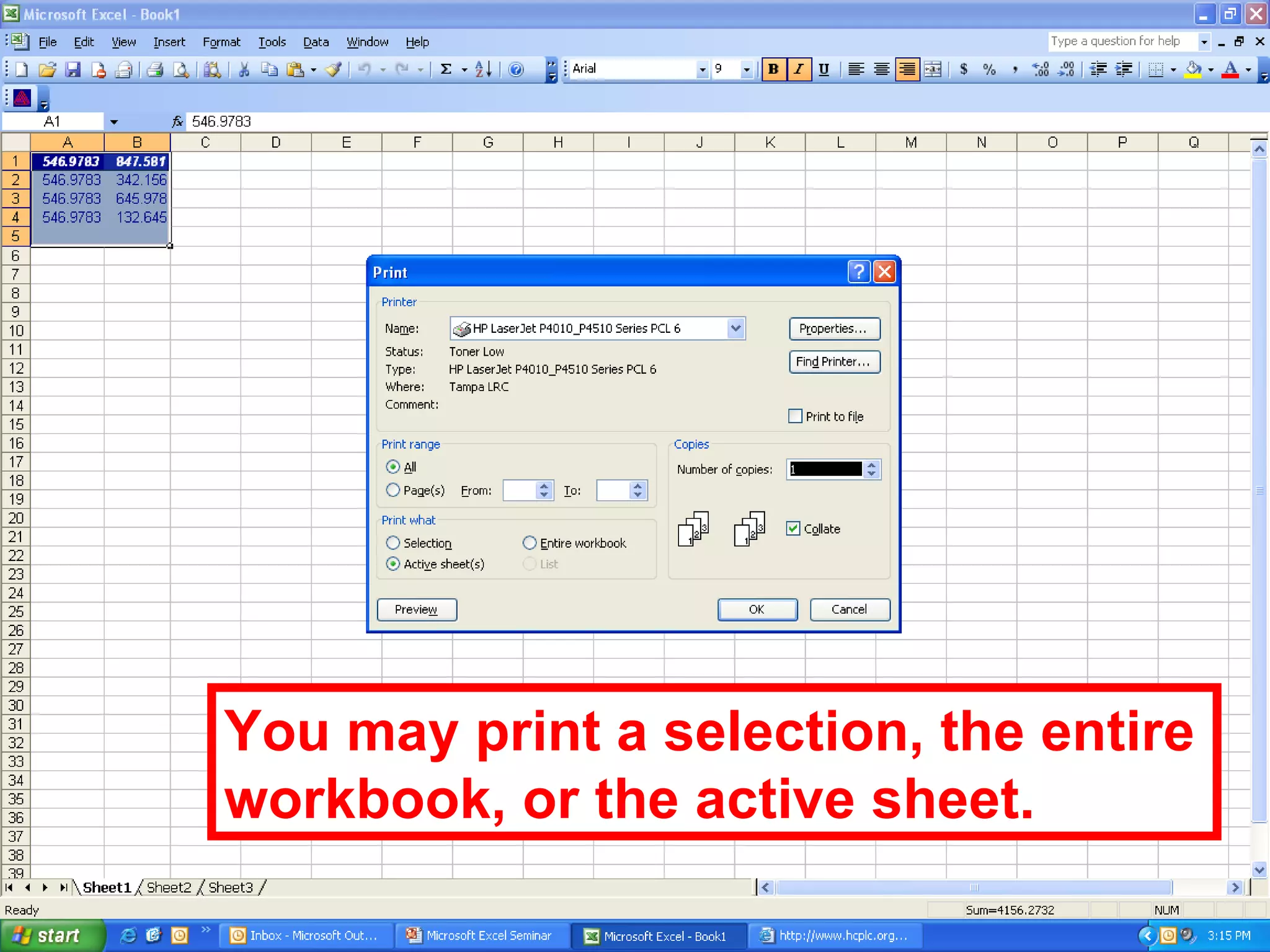
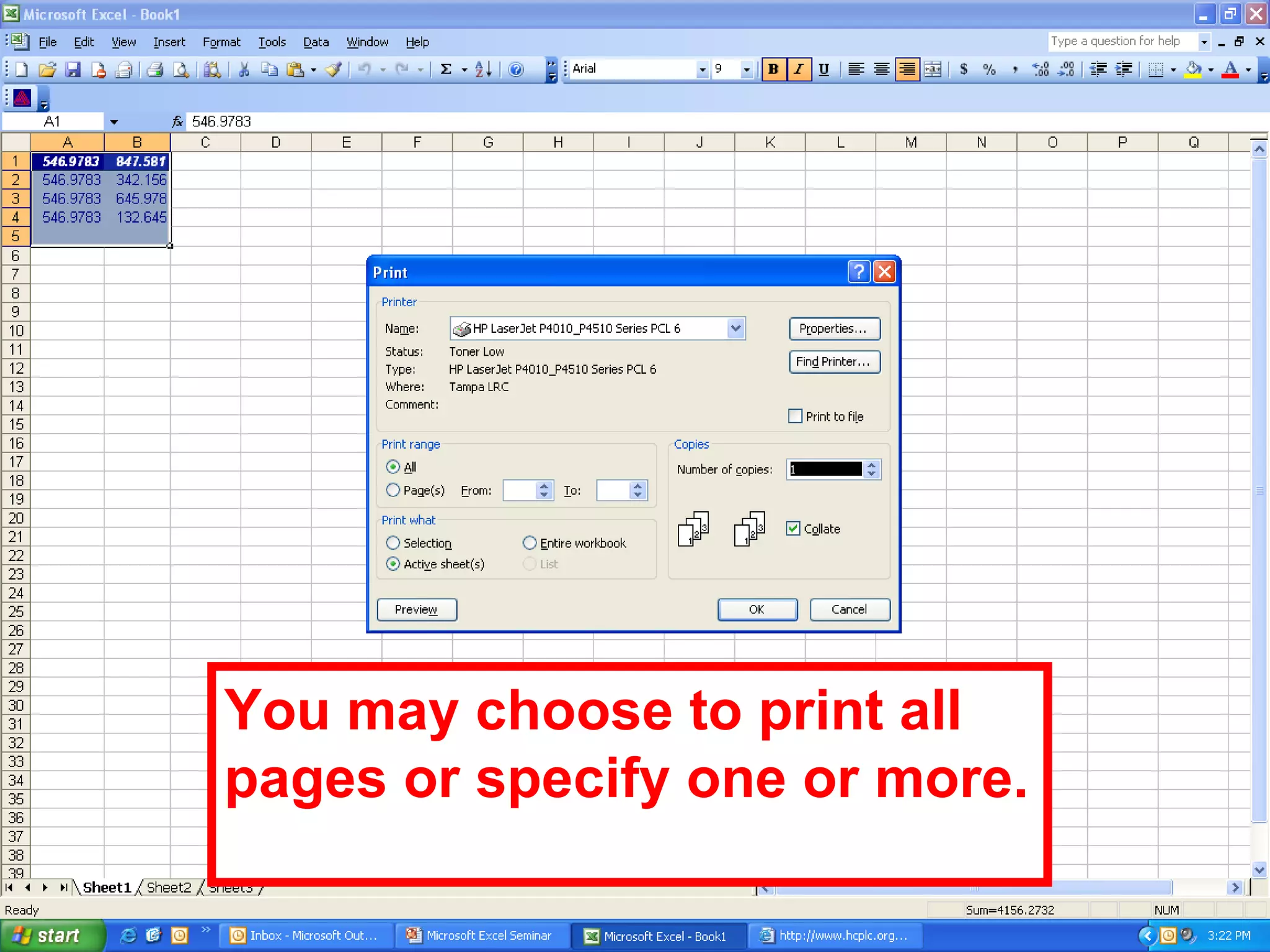
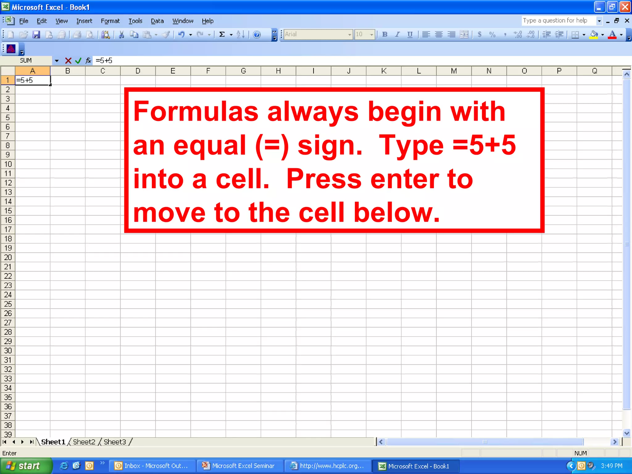
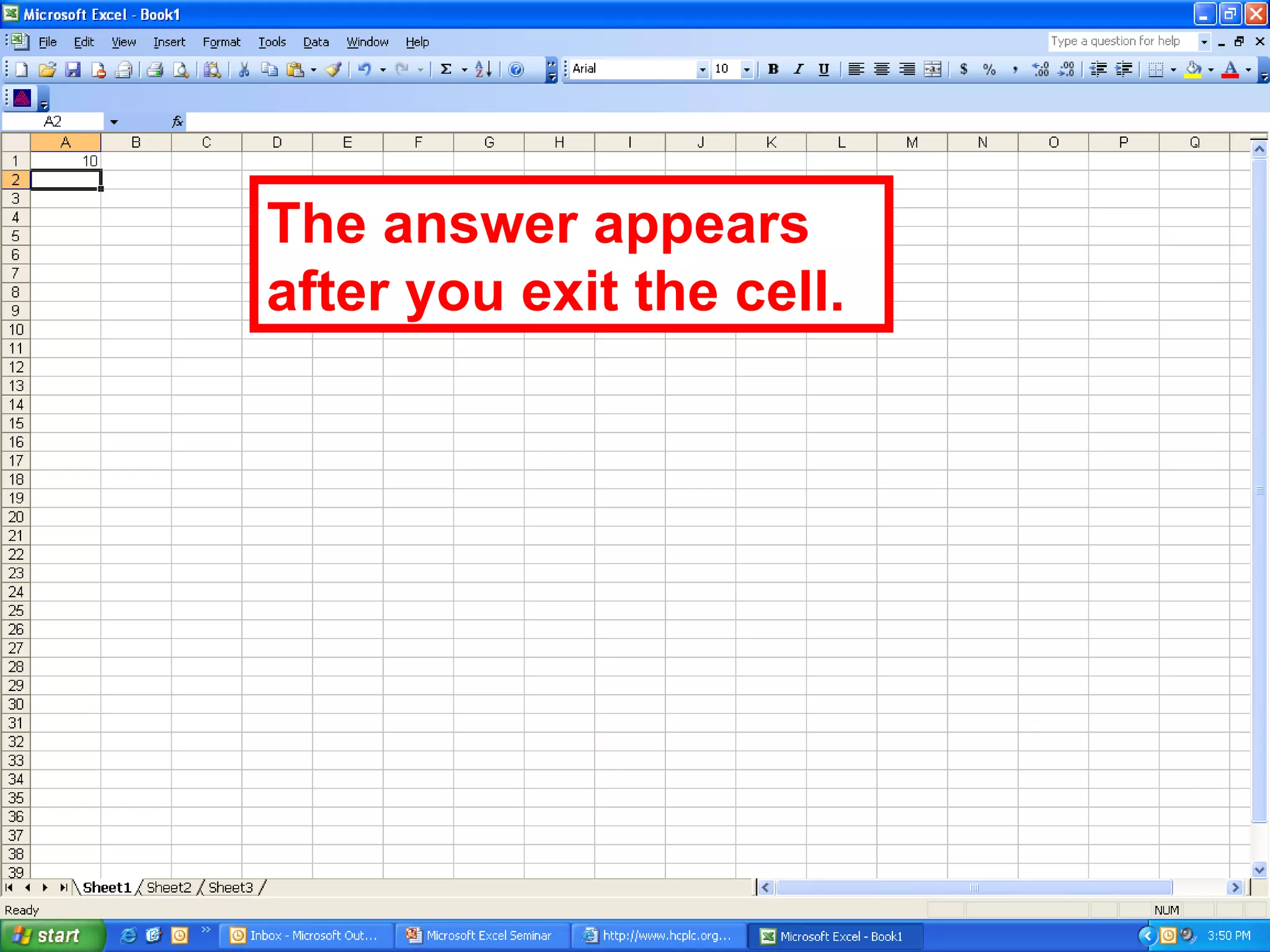

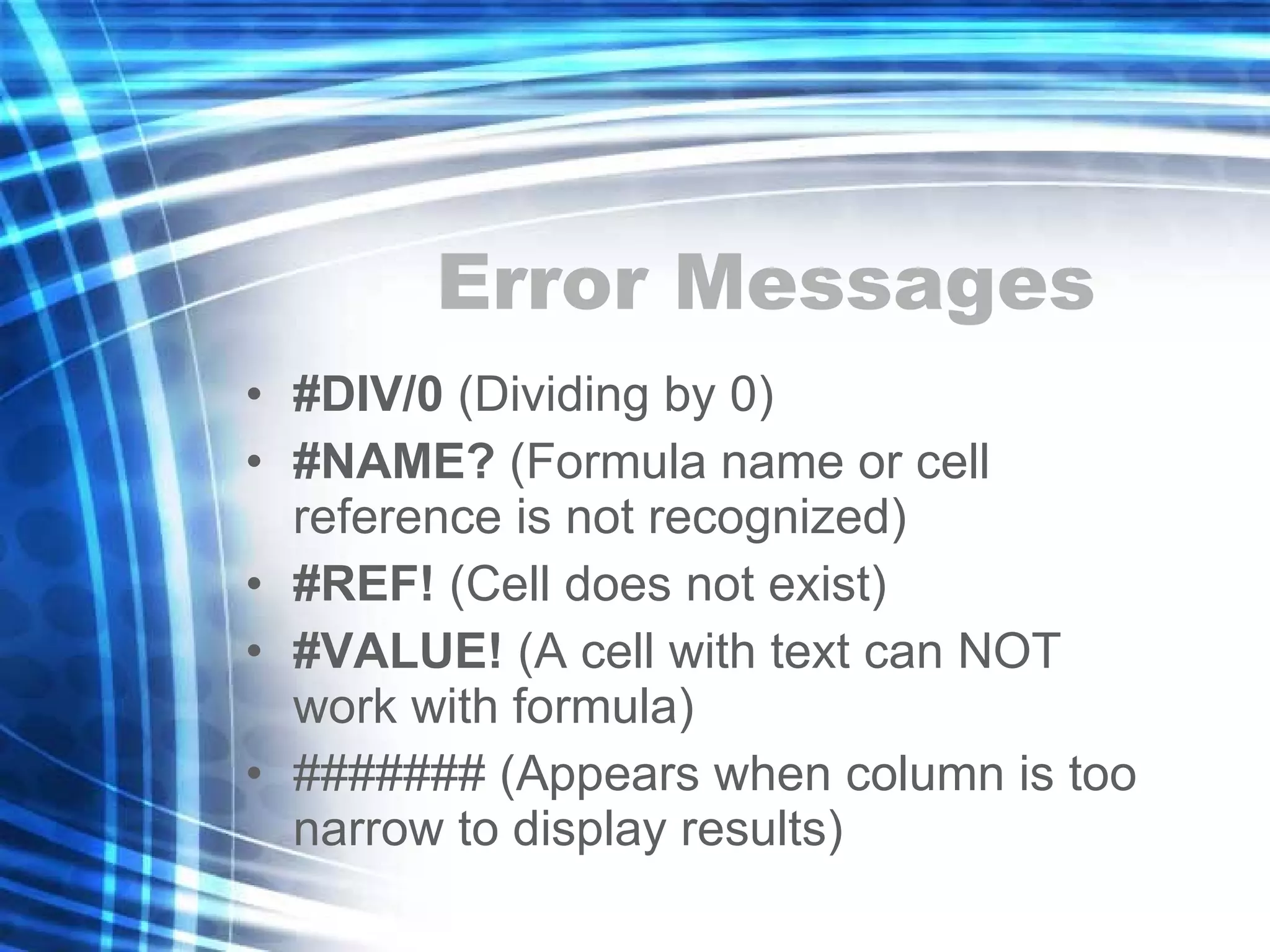

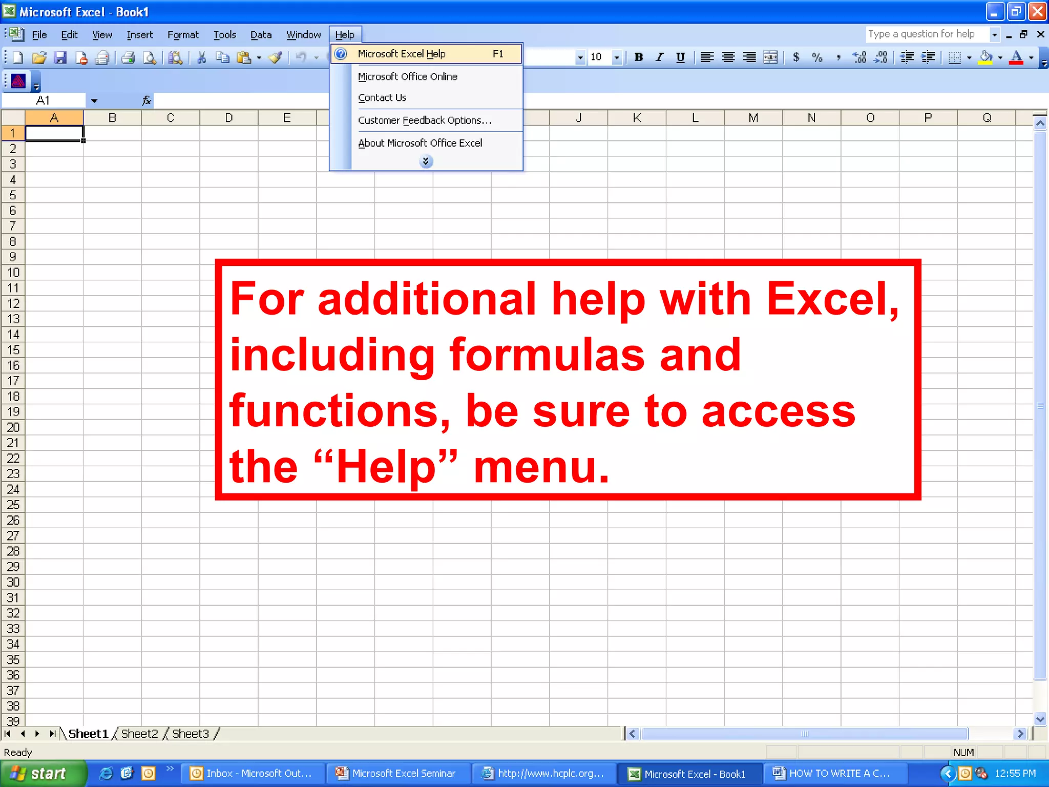


This document provides an overview of the basic functions and features of Microsoft Excel. It explains how to navigate an Excel worksheet and describes the different areas like cells, columns, rows, and worksheets. It also covers how to enter and format text and numeric data, perform calculations with formulas, and print or modify a worksheet. Common tasks like inserting or deleting cells/rows/columns, copying and pasting data, and using auto-fill are demonstrated. Finally, it introduces basic formulas and functions in Excel.


![SHS_Core_CAE_Q3_LE1 FOR THIRD [FINAL].pdf](https://cdn.slidesharecdn.com/ss_thumbnails/shscorecaeq3le1final-251116055110-e3081055-thumbnail.jpg?width=640&height=640&fit=bounds)


