Downloaded 1,141 times


![Formulas
• Conditional Math
=SumIf(range, criteria, [sum range])
=CountIf(range, criteria)
• What if there was no AverageIf, how would I find the average?
=SumIf(range, criteria, [sum range])/CountIf(range, criteria)
Excel Excellence 22](https://image.slidesharecdn.com/cssc01-formulas-141012123146-conversion-gate01/75/Excel-Excellence-Microsoft-Excel-training-that-sticks-Formulas-22-2048.jpg)
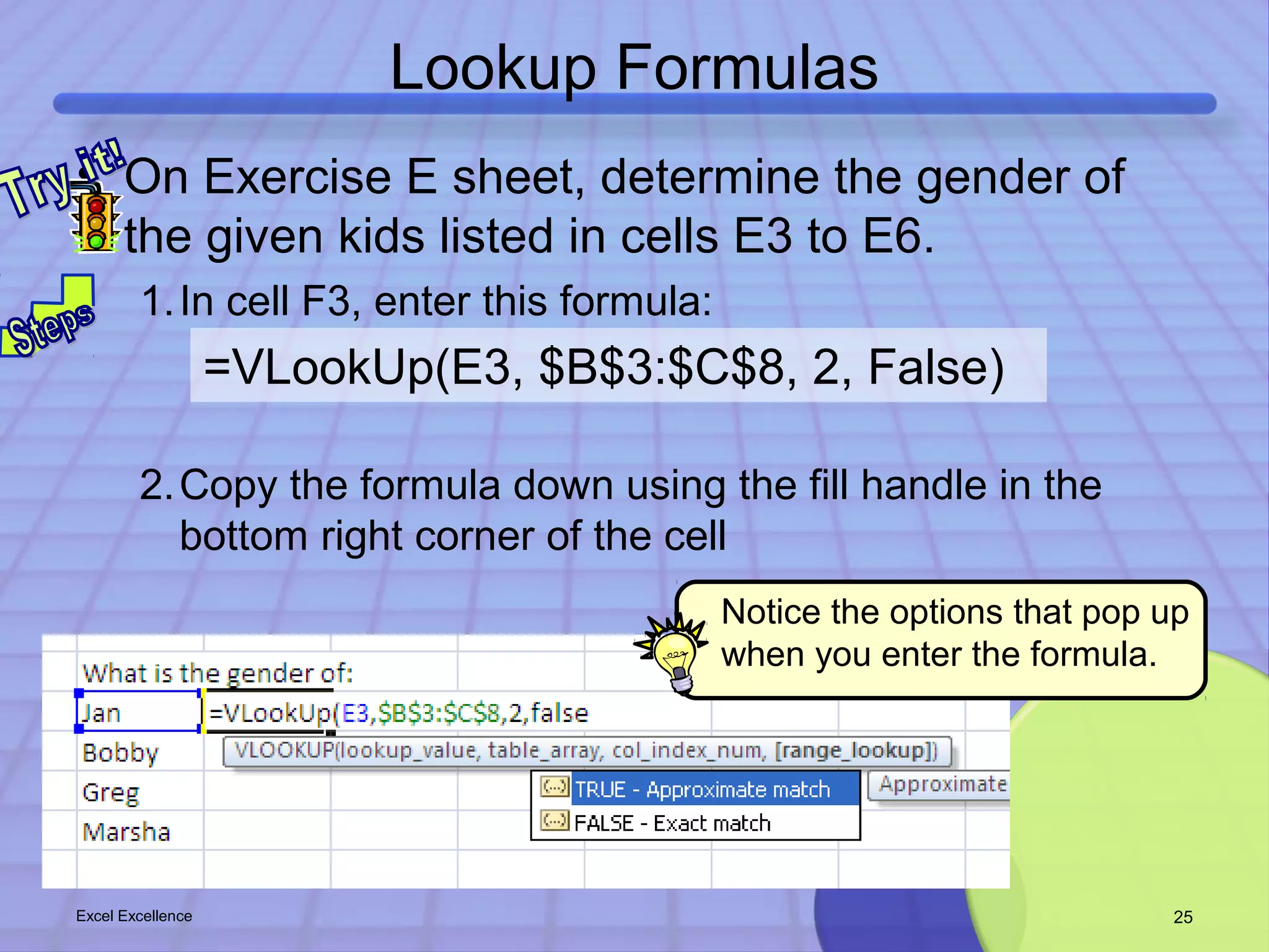
![Lookup Formulas
• Basic formula:
Lookup(LookupValue,LookupVector,ResultVector)
• Variants:
Lookup(LookupValue,Array)
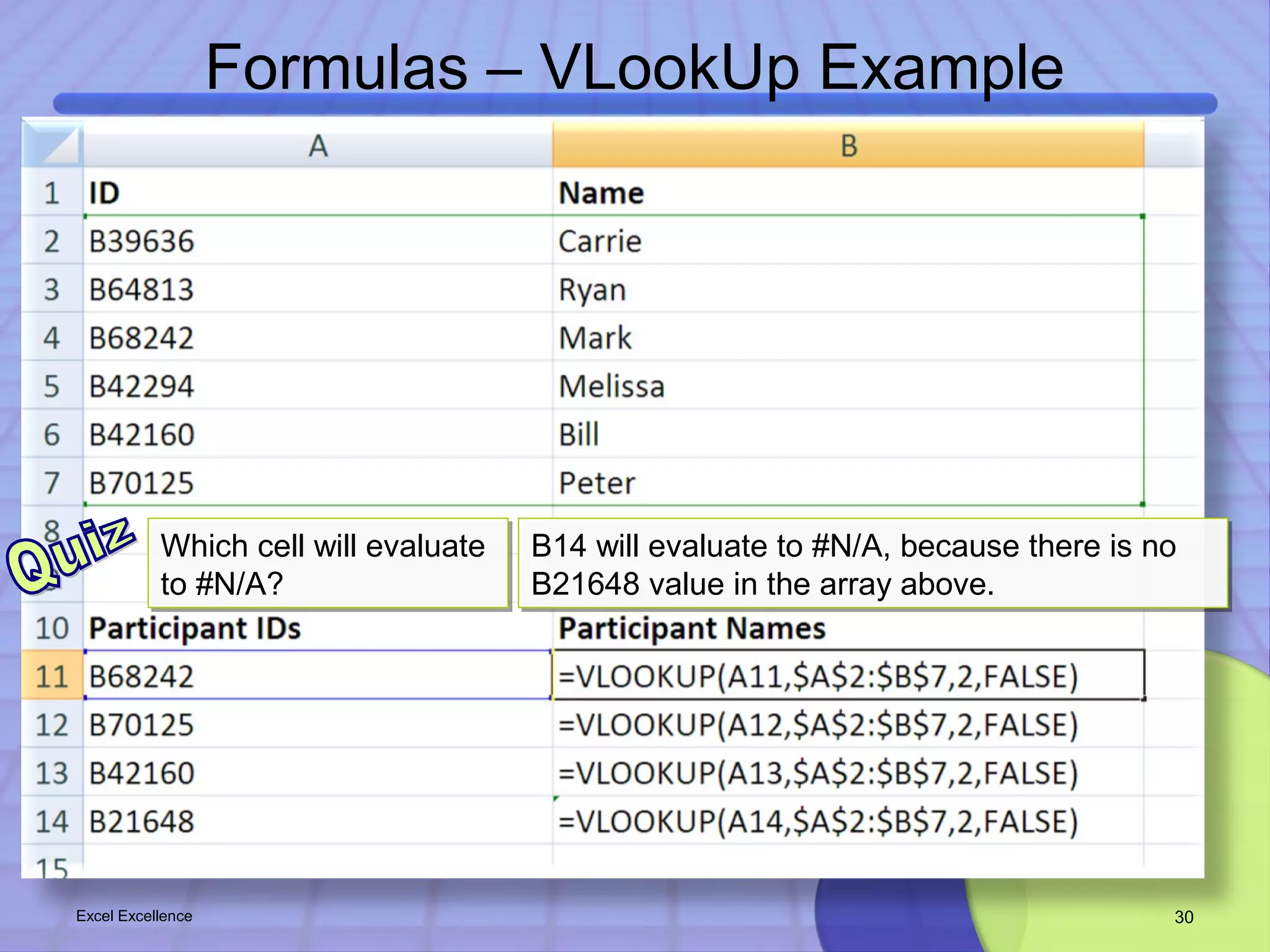
VLookUp(LookupValue, TableArray, ColIndexNum,
[RangeLookup])
HLookup
• Generally, you want to use FALSE as RangeLookup to ensure
you will get only exact matches
– WARNING: Values in LookupVector should be placed in
Ascending Order
– WARNING: If Lookup doesn’t find the LookupValue, it
matches the largest value in LookupVector that is less than
LookupValue
Excel Excellence 24](https://image.slidesharecdn.com/cssc01-formulas-141012123146-conversion-gate01/75/Excel-Excellence-Microsoft-Excel-training-that-sticks-Formulas-24-2048.jpg)


![Formulas
• Conditional Math
=SumIf(range, criteria, [sum range])
=CountIf(range, criteria)
• What if there was no AverageIf, how would I find the average?
=SumIf(range, criteria, [sum range])/CountIf(range, criteria)
Excel Excellence 22](https://crownmelresort.com/image.slidesharecdn.com/cssc01-formulas-141012123146-conversion-gate01/75/Excel-Excellence-Microsoft-Excel-training-that-sticks-Formulas-22-2048.jpg)

![Lookup Formulas
• Basic formula:
Lookup(LookupValue,LookupVector,ResultVector)
• Variants:
Lookup(LookupValue,Array)
VLookUp(LookupValue, TableArray, ColIndexNum,
[RangeLookup])
HLookup
• Generally, you want to use FALSE as RangeLookup to ensure
you will get only exact matches
– WARNING: Values in LookupVector should be placed in
Ascending Order
– WARNING: If Lookup doesn’t find the LookupValue, it
matches the largest value in LookupVector that is less than
LookupValue
Excel Excellence 24](https://crownmelresort.com/image.slidesharecdn.com/cssc01-formulas-141012123146-conversion-gate01/75/Excel-Excellence-Microsoft-Excel-training-that-sticks-Formulas-24-2048.jpg)


The document outlines an Excel training course led by Laura Winger, detailing her background and the course content, which includes key Excel concepts such as formulas, references, conditional math, and string functions. It emphasizes active participation, practice, and application of skills learned, as well as providing exercises to reinforce understanding. Furthermore, it highlights the use of lookup functions and date manipulations for effective data analysis.