![Games Chapter 6 Dr. Mustafa Jarrar University of Birzeit [email_address] www.jarrar.info Lecture Notes, Advanced Artificial Intelligence (SCOM7341) University of Birzeit 2 nd Semester, 2011 Advanced Artificial Intelligence (SCOM7341)](https://image.slidesharecdn.com/jarrar-lecturenotes-aai-2011s-ch6-games-110917072113-phpapp01/75/Jarrar-lecture-notes-aai-2011s-ch6-games-1-2048.jpg)


![Alpha-Beta Example 2 we assume a depth-first, left-to-right search as basic strategy the range of the possible values for each node are indicated initially [-∞, +∞] from Max ’s or Min ’s perspective these local values reflect the values of the sub-trees in that node; the global values and are the best overall choices so far for Max or Min [-∞, +∞] [-∞, +∞] best choice for Max ? best choice for Min ? Max Min](https://image.slidesharecdn.com/jarrar-lecturenotes-aai-2011s-ch6-games-110917072113-phpapp01/75/Jarrar-lecture-notes-aai-2011s-ch6-games-36-2048.jpg)
![Alpha-Beta Example 2 Max Min [-∞, 7] [-∞, +∞] best choice for Max ? best choice for Min 7 7](https://image.slidesharecdn.com/jarrar-lecturenotes-aai-2011s-ch6-games-110917072113-phpapp01/75/Jarrar-lecture-notes-aai-2011s-ch6-games-37-2048.jpg)
![Alpha-Beta Example 2 Max Min [-∞, 6] [-∞, +∞] best choice for Max ? best choice for Min 6 7 6](https://image.slidesharecdn.com/jarrar-lecturenotes-aai-2011s-ch6-games-110917072113-phpapp01/75/Jarrar-lecture-notes-aai-2011s-ch6-games-38-2048.jpg)
![Alpha-Beta Example 2 Max Min 5 [5, +∞] best choice for Max 5 best choice for Min 5 7 6 5 Min obtains the third value from a successor node this is the last value from this sub-tree, and the exact value is known Max now has a value for its first successor node, but hopes that something better might still come](https://image.slidesharecdn.com/jarrar-lecturenotes-aai-2011s-ch6-games-110917072113-phpapp01/75/Jarrar-lecture-notes-aai-2011s-ch6-games-39-2048.jpg)
![Alpha-Beta Example 2 Max Min [-∞, 5] [5, +∞] best choice for Max 5 best choice for Min 3 7 6 5 Min continues with the next sub-tree, and gets a better value Max has a better choice from its perspective, however, and will not consider a move in the sub-tree currently explored by Min initially [-∞, +∞] [-∞,3] 3](https://image.slidesharecdn.com/jarrar-lecturenotes-aai-2011s-ch6-games-110917072113-phpapp01/75/Jarrar-lecture-notes-aai-2011s-ch6-games-40-2048.jpg)
![Alpha-Beta Example 2 Max Min [-∞, 5] [5, +∞] best choice for Max 5 best choice for Min 3 7 6 5 Min knows that Max won’t consider a move to this sub-tree, and abandons it this is a case of pruning, indicated by [-∞,3] 3](https://image.slidesharecdn.com/jarrar-lecturenotes-aai-2011s-ch6-games-110917072113-phpapp01/75/Jarrar-lecture-notes-aai-2011s-ch6-games-41-2048.jpg)
![Alpha-Beta Example 2 Max Min [-∞, 5] [5, +∞] best choice for Max 5 best choice for Min 3 7 6 5 Min explores the next sub-tree, and finds a value that is worse than the other nodes at this level if Min is not able to find something lower, then Max will choose this branch, so Min must explore more successor nodes [-∞,3] 3 [-∞,6] 6](https://image.slidesharecdn.com/jarrar-lecturenotes-aai-2011s-ch6-games-110917072113-phpapp01/75/Jarrar-lecture-notes-aai-2011s-ch6-games-42-2048.jpg)
![Alpha-Beta Example 2 Max Min [-∞, 5] [5, +∞] best choice for Max 5 best choice for Min 3 7 6 5 Min is lucky, and finds a value that is the same as the current worst value at this level Max can choose this branch, or the other branch with the same value [-∞,3] 3 [-∞,5] 6 5](https://image.slidesharecdn.com/jarrar-lecturenotes-aai-2011s-ch6-games-110917072113-phpapp01/75/Jarrar-lecture-notes-aai-2011s-ch6-games-43-2048.jpg)
![Alpha-Beta Example 2 Max Min [-∞, 5] 5 best choice for Max 5 best choice for Min 3 7 6 5 Min could continue searching this sub-tree to see if there is a value that is less than the current worst alternative in order to give Max as few choices as possible this depends on the specific implementation Max knows the best value for its sub-tree [-∞,3] 3 [-∞,5] 6 5](https://image.slidesharecdn.com/jarrar-lecturenotes-aai-2011s-ch6-games-110917072113-phpapp01/75/Jarrar-lecture-notes-aai-2011s-ch6-games-44-2048.jpg)


![Games Chapter 6 Dr. Mustafa Jarrar University of Birzeit [email_address] www.jarrar.info Lecture Notes, Advanced Artificial Intelligence (SCOM7341) University of Birzeit 2 nd Semester, 2011 Advanced Artificial Intelligence (SCOM7341)](https://crownmelresort.com/image.slidesharecdn.com/jarrar-lecturenotes-aai-2011s-ch6-games-110917072113-phpapp01/75/Jarrar-lecture-notes-aai-2011s-ch6-games-1-2048.jpg)


![Alpha-Beta Example 2 we assume a depth-first, left-to-right search as basic strategy the range of the possible values for each node are indicated initially [-∞, +∞] from Max ’s or Min ’s perspective these local values reflect the values of the sub-trees in that node; the global values and are the best overall choices so far for Max or Min [-∞, +∞] [-∞, +∞] best choice for Max ? best choice for Min ? Max Min](https://crownmelresort.com/image.slidesharecdn.com/jarrar-lecturenotes-aai-2011s-ch6-games-110917072113-phpapp01/75/Jarrar-lecture-notes-aai-2011s-ch6-games-36-2048.jpg)
![Alpha-Beta Example 2 Max Min [-∞, 7] [-∞, +∞] best choice for Max ? best choice for Min 7 7](https://crownmelresort.com/image.slidesharecdn.com/jarrar-lecturenotes-aai-2011s-ch6-games-110917072113-phpapp01/75/Jarrar-lecture-notes-aai-2011s-ch6-games-37-2048.jpg)
![Alpha-Beta Example 2 Max Min [-∞, 6] [-∞, +∞] best choice for Max ? best choice for Min 6 7 6](https://crownmelresort.com/image.slidesharecdn.com/jarrar-lecturenotes-aai-2011s-ch6-games-110917072113-phpapp01/75/Jarrar-lecture-notes-aai-2011s-ch6-games-38-2048.jpg)
![Alpha-Beta Example 2 Max Min 5 [5, +∞] best choice for Max 5 best choice for Min 5 7 6 5 Min obtains the third value from a successor node this is the last value from this sub-tree, and the exact value is known Max now has a value for its first successor node, but hopes that something better might still come](https://crownmelresort.com/image.slidesharecdn.com/jarrar-lecturenotes-aai-2011s-ch6-games-110917072113-phpapp01/75/Jarrar-lecture-notes-aai-2011s-ch6-games-39-2048.jpg)
![Alpha-Beta Example 2 Max Min [-∞, 5] [5, +∞] best choice for Max 5 best choice for Min 3 7 6 5 Min continues with the next sub-tree, and gets a better value Max has a better choice from its perspective, however, and will not consider a move in the sub-tree currently explored by Min initially [-∞, +∞] [-∞,3] 3](https://crownmelresort.com/image.slidesharecdn.com/jarrar-lecturenotes-aai-2011s-ch6-games-110917072113-phpapp01/75/Jarrar-lecture-notes-aai-2011s-ch6-games-40-2048.jpg)
![Alpha-Beta Example 2 Max Min [-∞, 5] [5, +∞] best choice for Max 5 best choice for Min 3 7 6 5 Min knows that Max won’t consider a move to this sub-tree, and abandons it this is a case of pruning, indicated by [-∞,3] 3](https://crownmelresort.com/image.slidesharecdn.com/jarrar-lecturenotes-aai-2011s-ch6-games-110917072113-phpapp01/75/Jarrar-lecture-notes-aai-2011s-ch6-games-41-2048.jpg)
![Alpha-Beta Example 2 Max Min [-∞, 5] [5, +∞] best choice for Max 5 best choice for Min 3 7 6 5 Min explores the next sub-tree, and finds a value that is worse than the other nodes at this level if Min is not able to find something lower, then Max will choose this branch, so Min must explore more successor nodes [-∞,3] 3 [-∞,6] 6](https://crownmelresort.com/image.slidesharecdn.com/jarrar-lecturenotes-aai-2011s-ch6-games-110917072113-phpapp01/75/Jarrar-lecture-notes-aai-2011s-ch6-games-42-2048.jpg)
![Alpha-Beta Example 2 Max Min [-∞, 5] [5, +∞] best choice for Max 5 best choice for Min 3 7 6 5 Min is lucky, and finds a value that is the same as the current worst value at this level Max can choose this branch, or the other branch with the same value [-∞,3] 3 [-∞,5] 6 5](https://crownmelresort.com/image.slidesharecdn.com/jarrar-lecturenotes-aai-2011s-ch6-games-110917072113-phpapp01/75/Jarrar-lecture-notes-aai-2011s-ch6-games-43-2048.jpg)
![Alpha-Beta Example 2 Max Min [-∞, 5] 5 best choice for Max 5 best choice for Min 3 7 6 5 Min could continue searching this sub-tree to see if there is a value that is less than the current worst alternative in order to give Max as few choices as possible this depends on the specific implementation Max knows the best value for its sub-tree [-∞,3] 3 [-∞,5] 6 5](https://crownmelresort.com/image.slidesharecdn.com/jarrar-lecturenotes-aai-2011s-ch6-games-110917072113-phpapp01/75/Jarrar-lecture-notes-aai-2011s-ch6-games-44-2048.jpg)


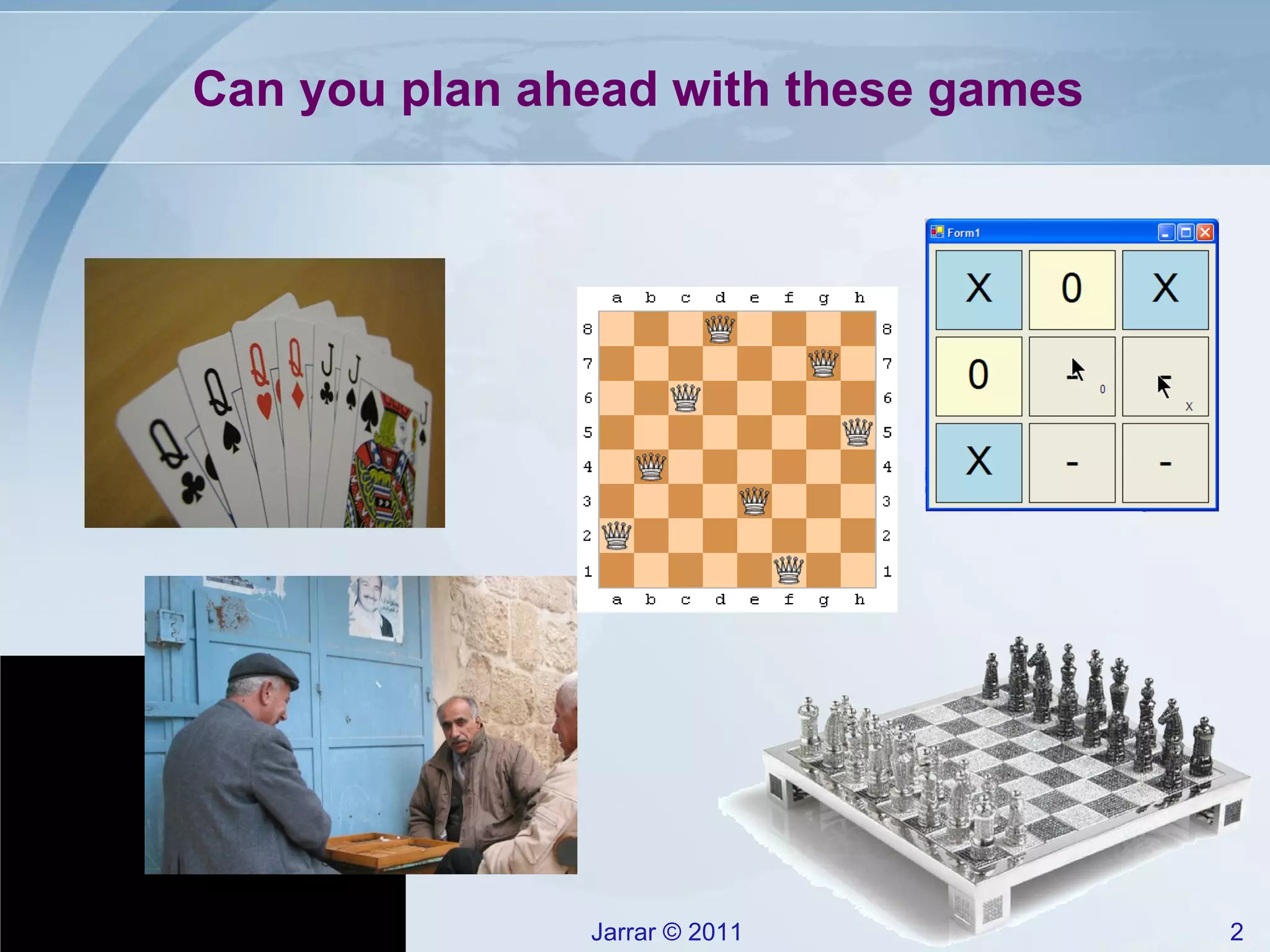
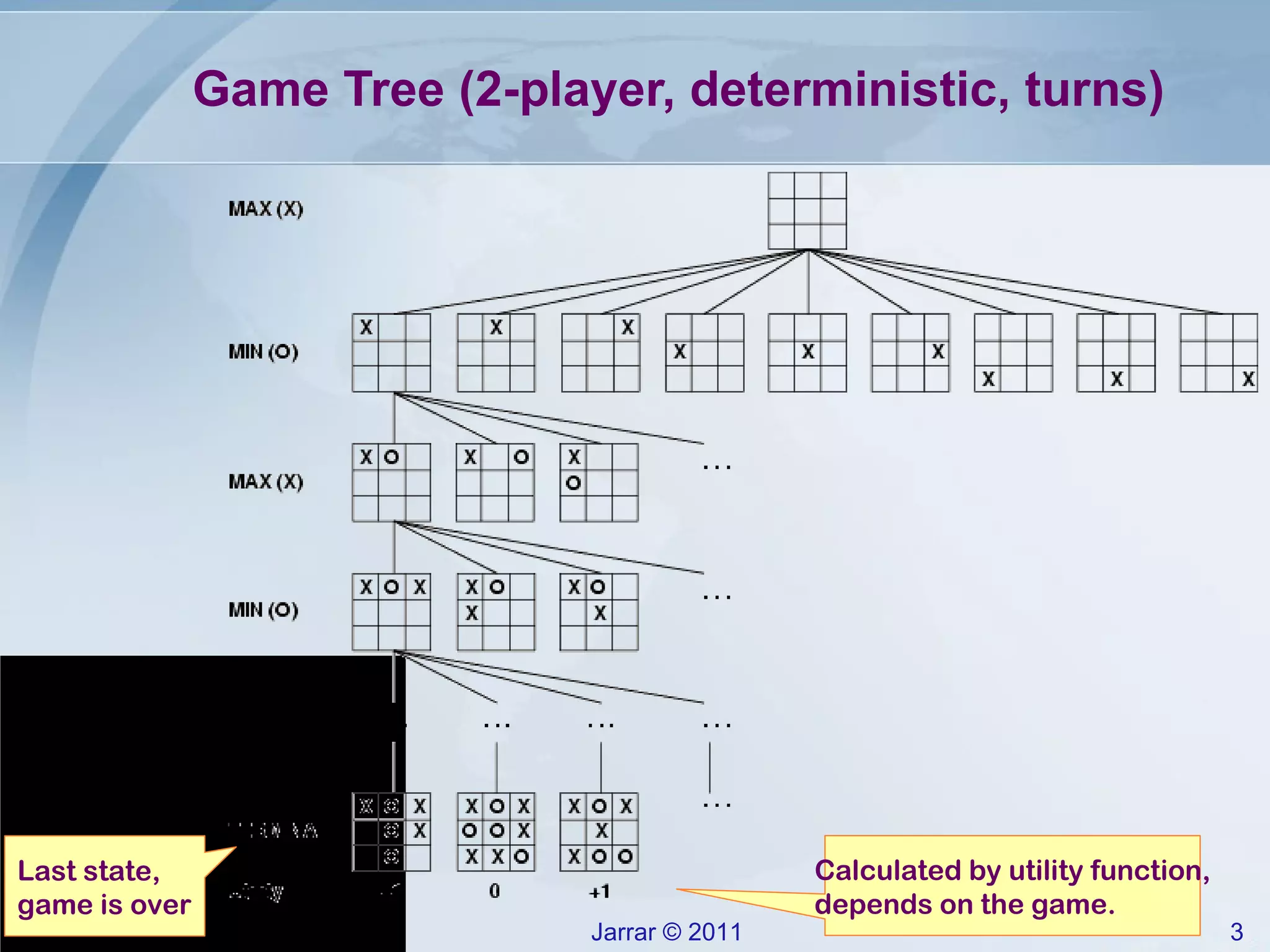
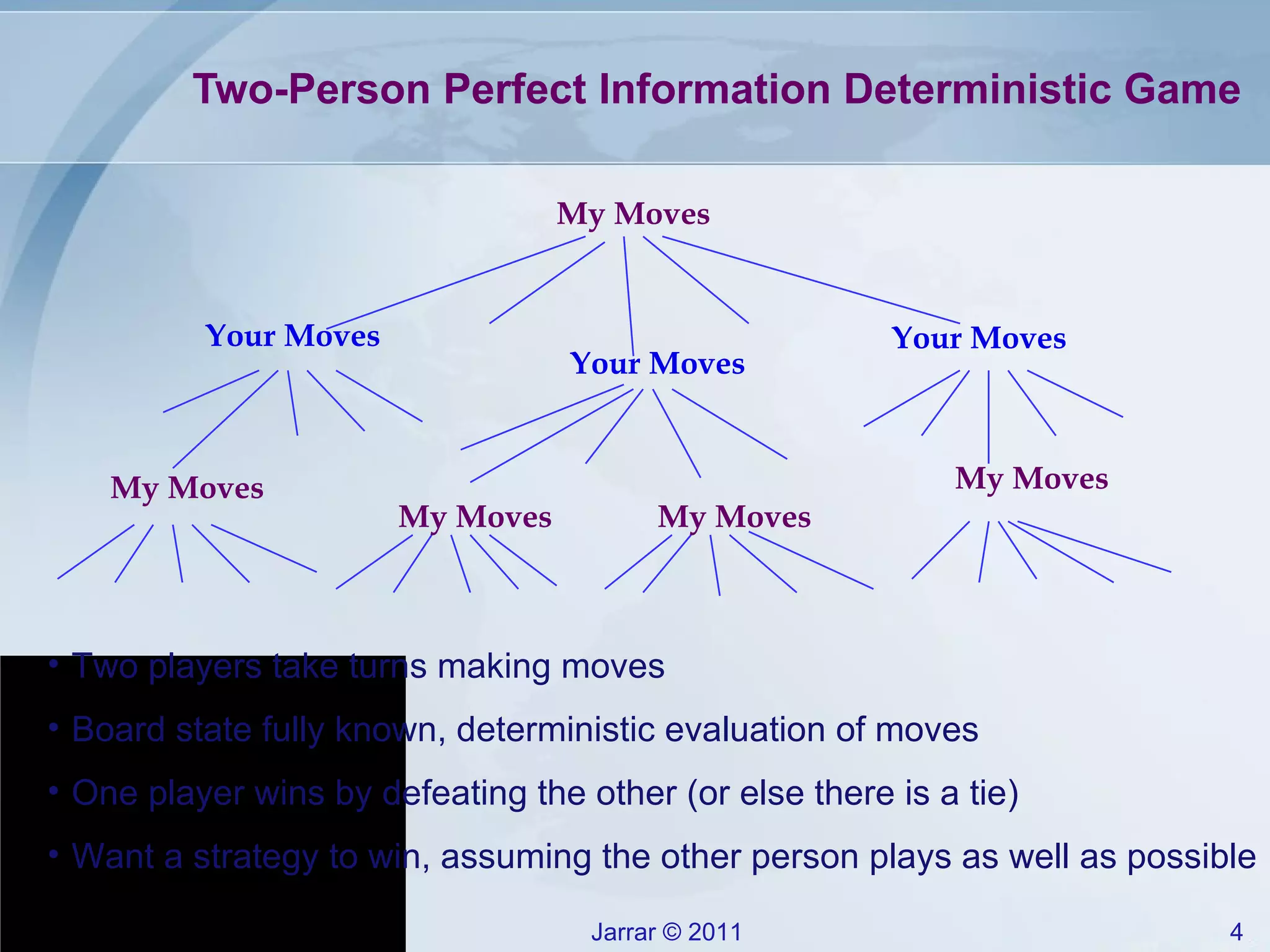
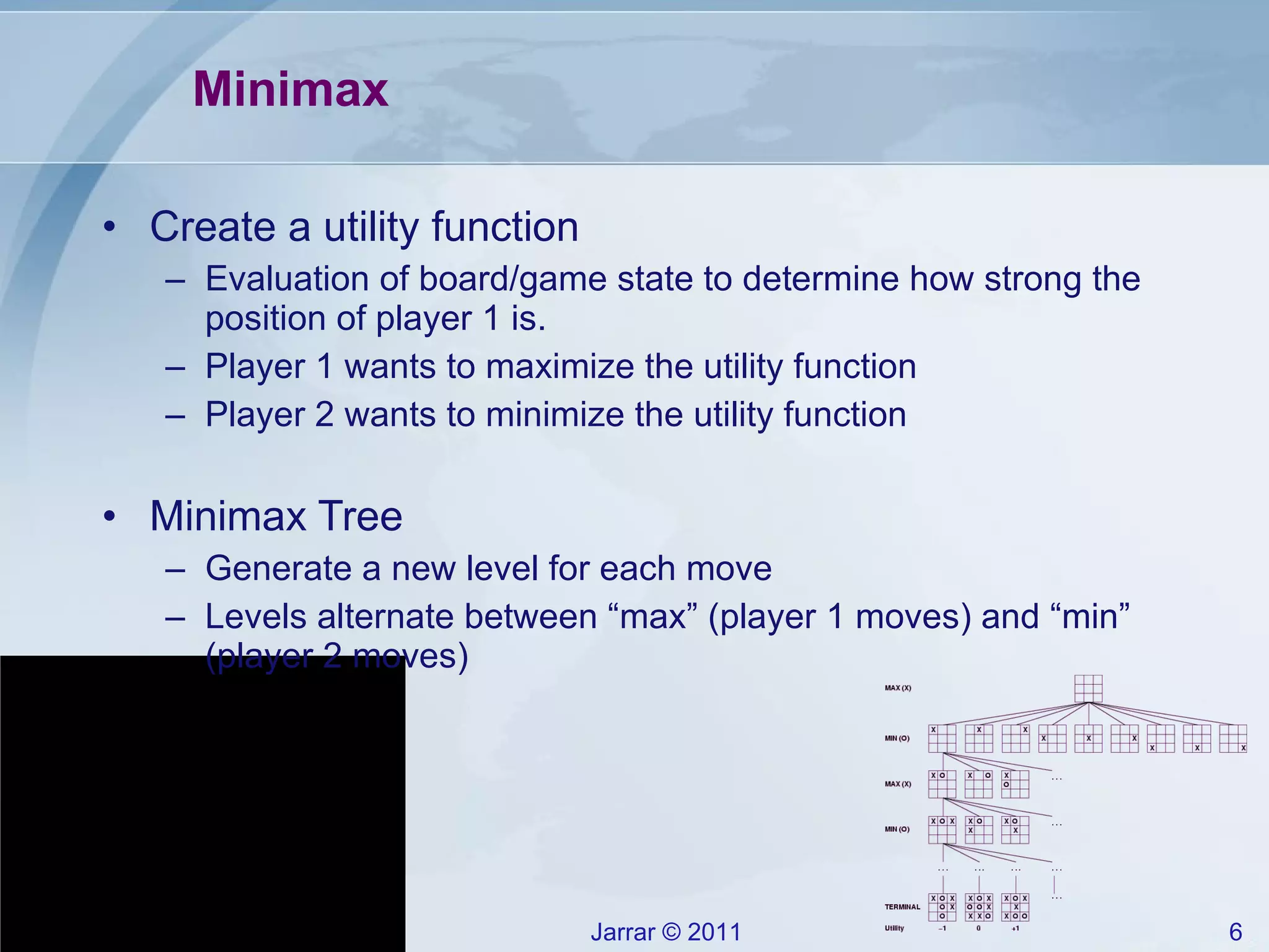
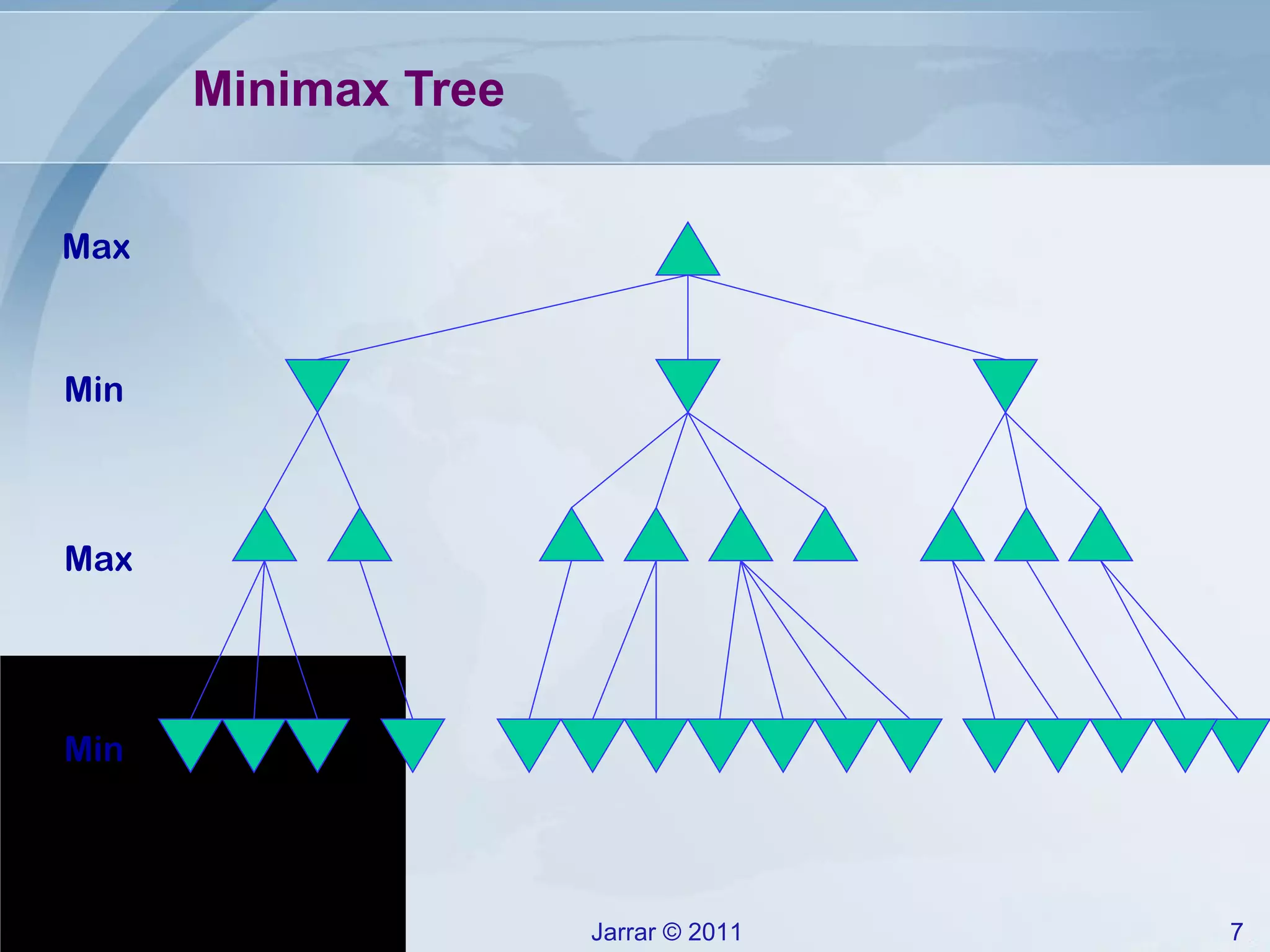
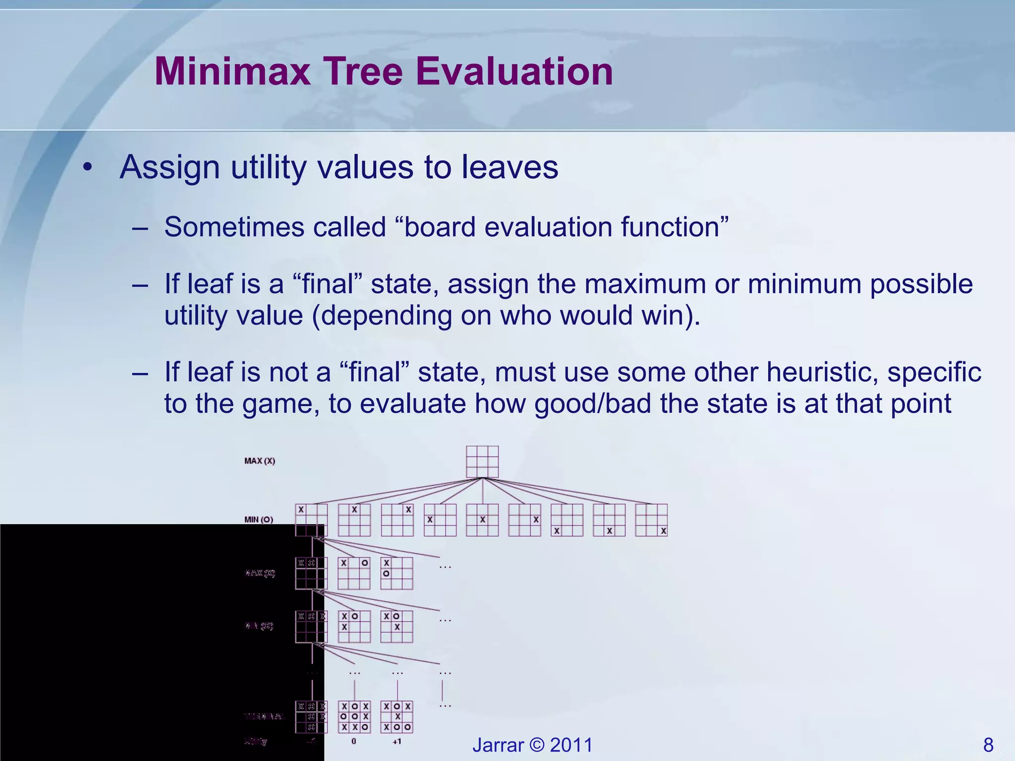
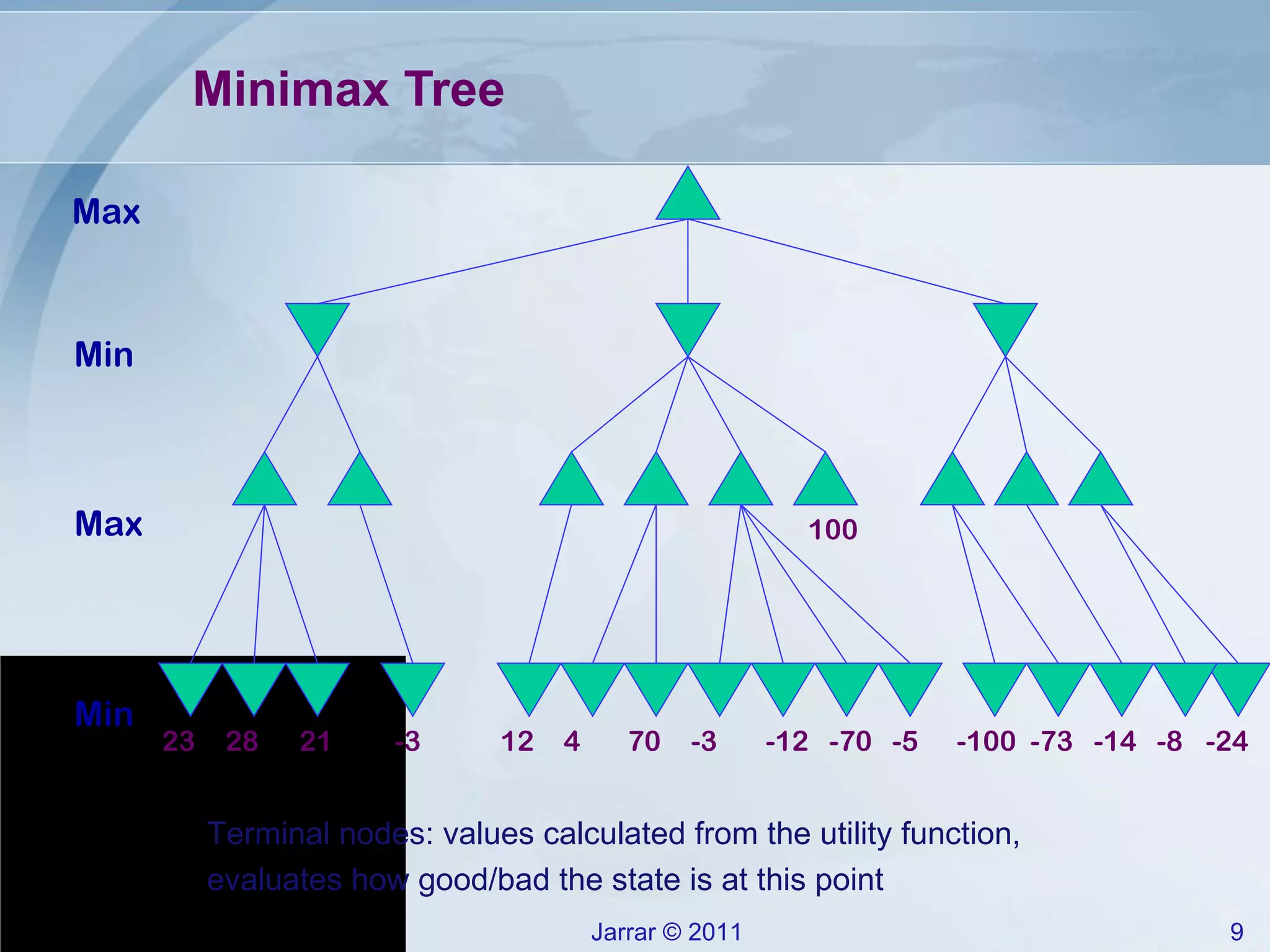
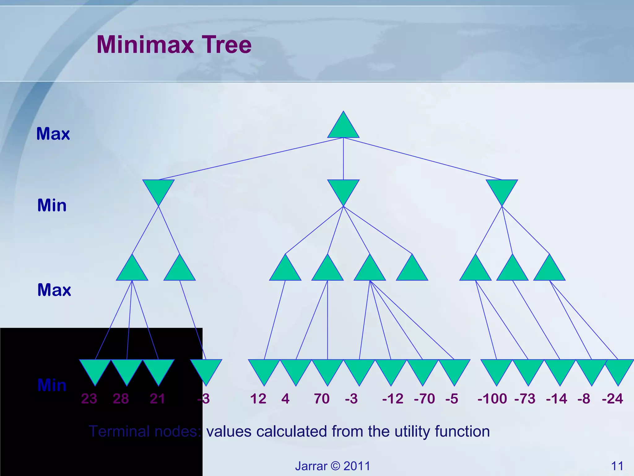
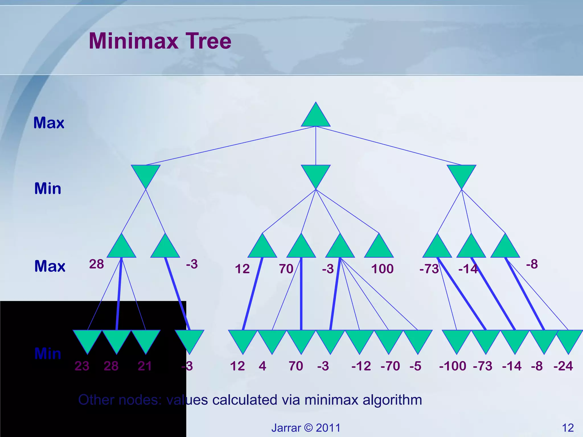
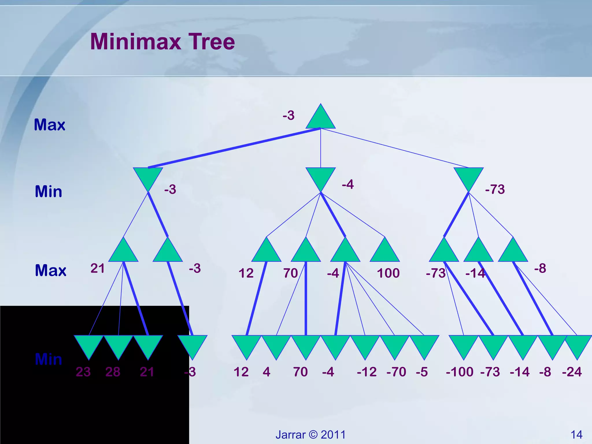
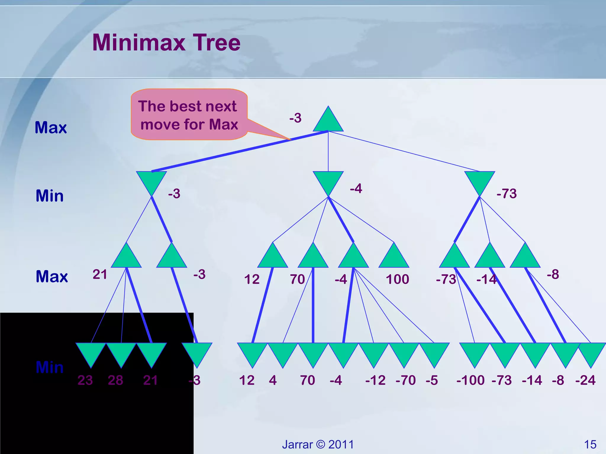
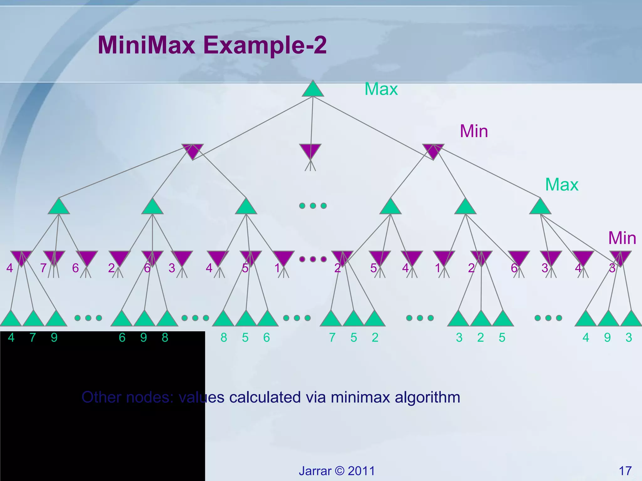
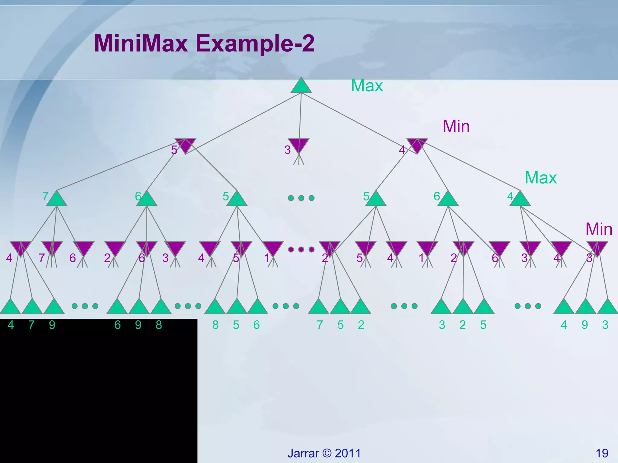
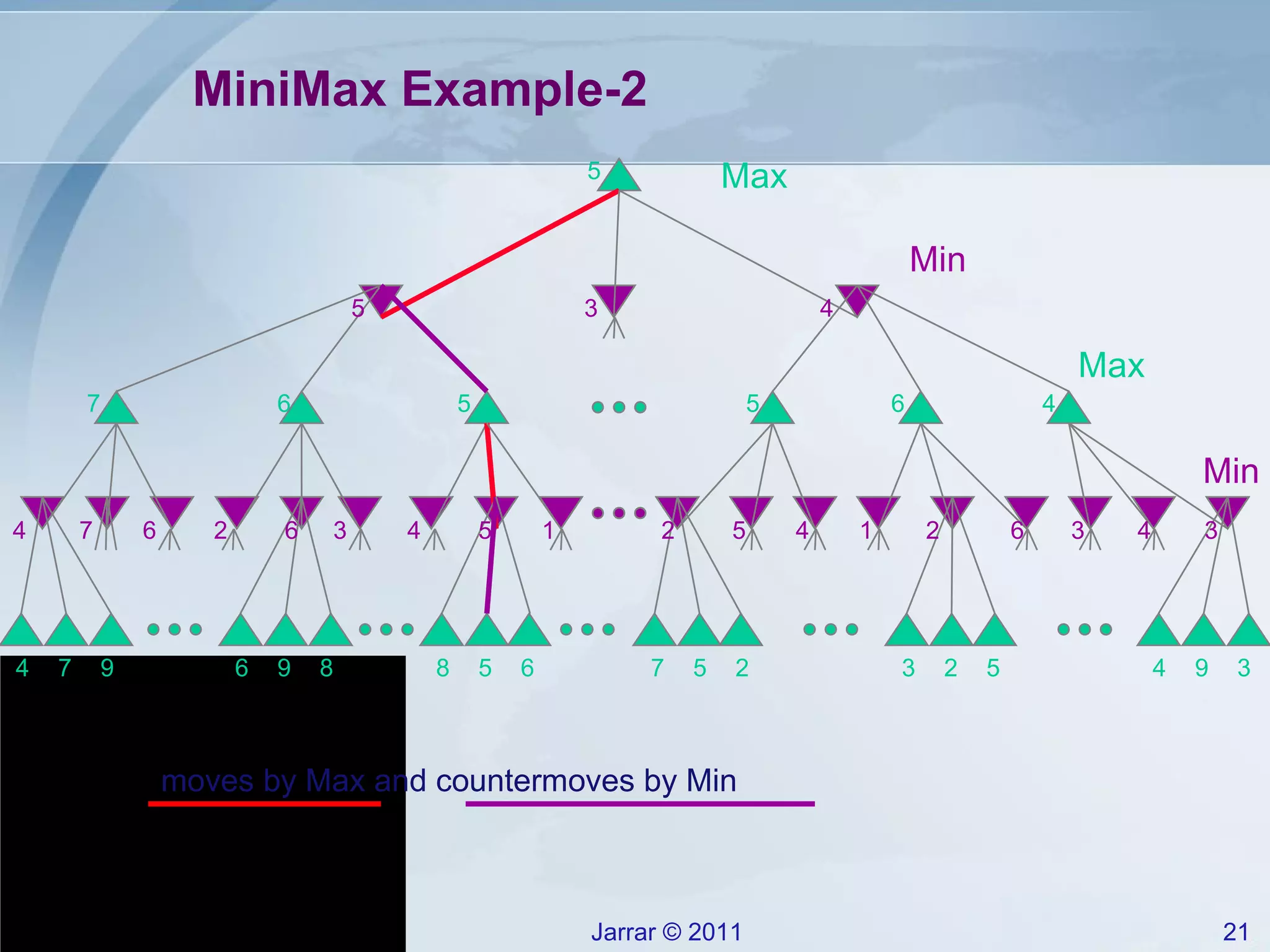
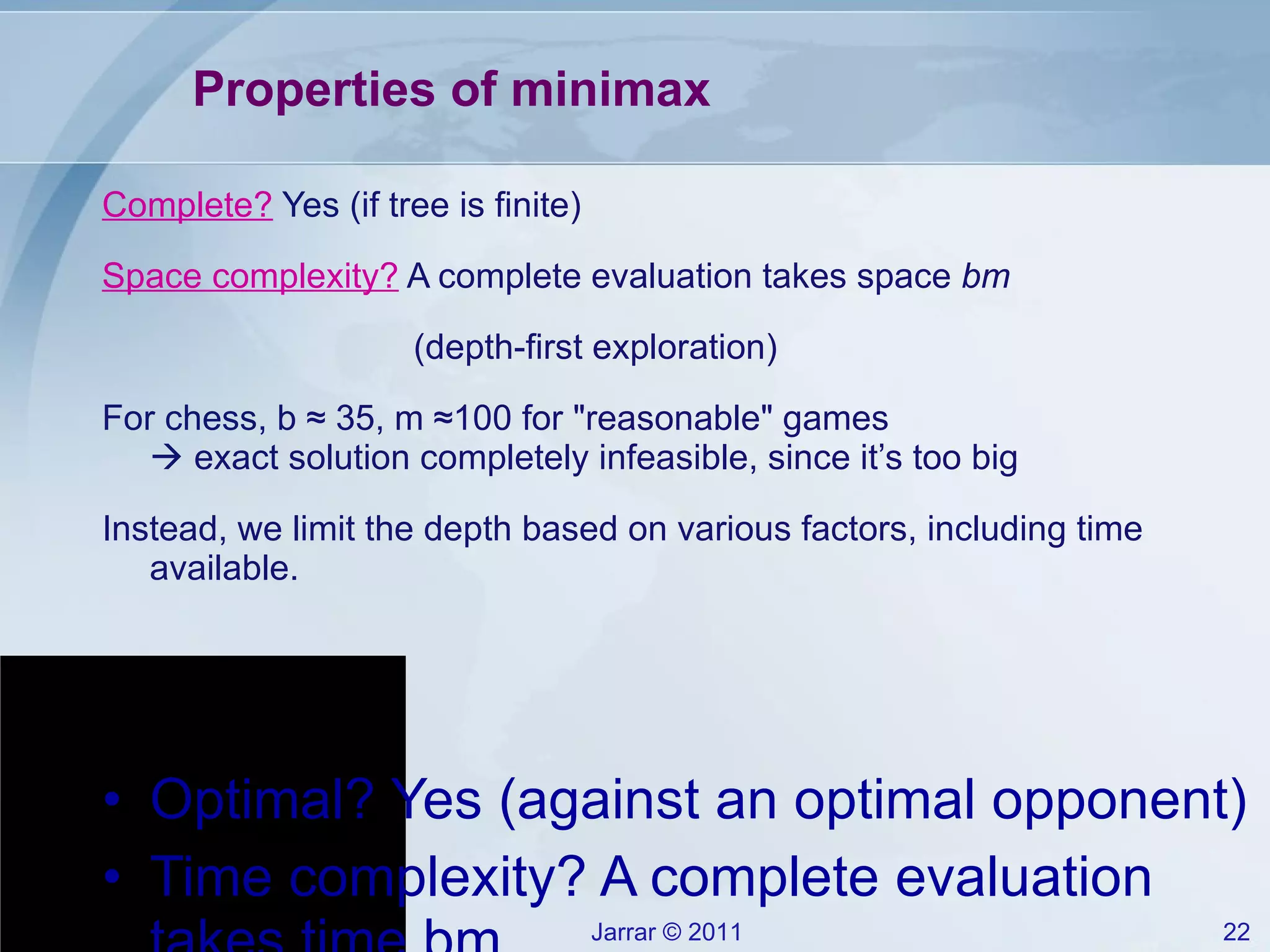
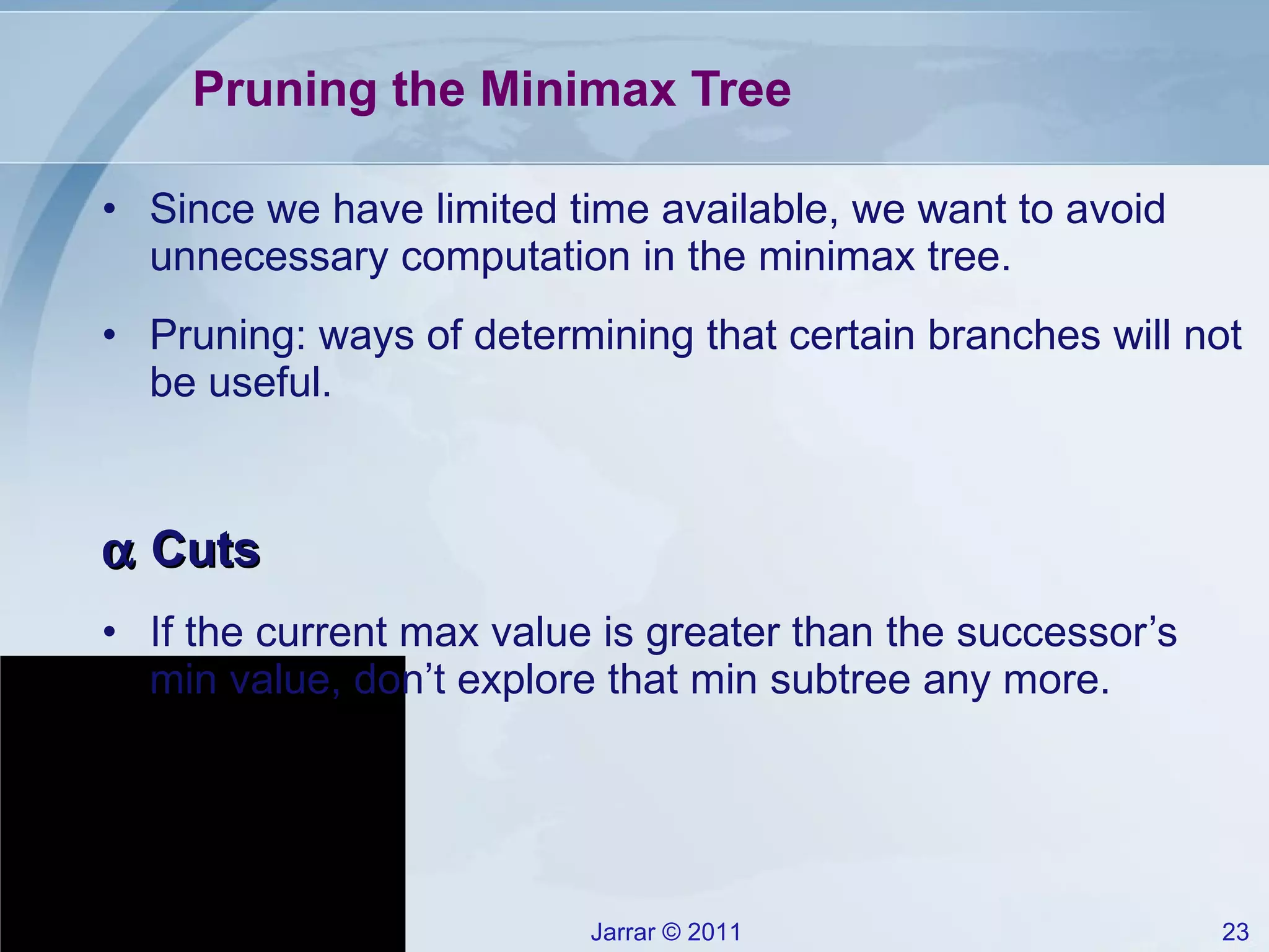
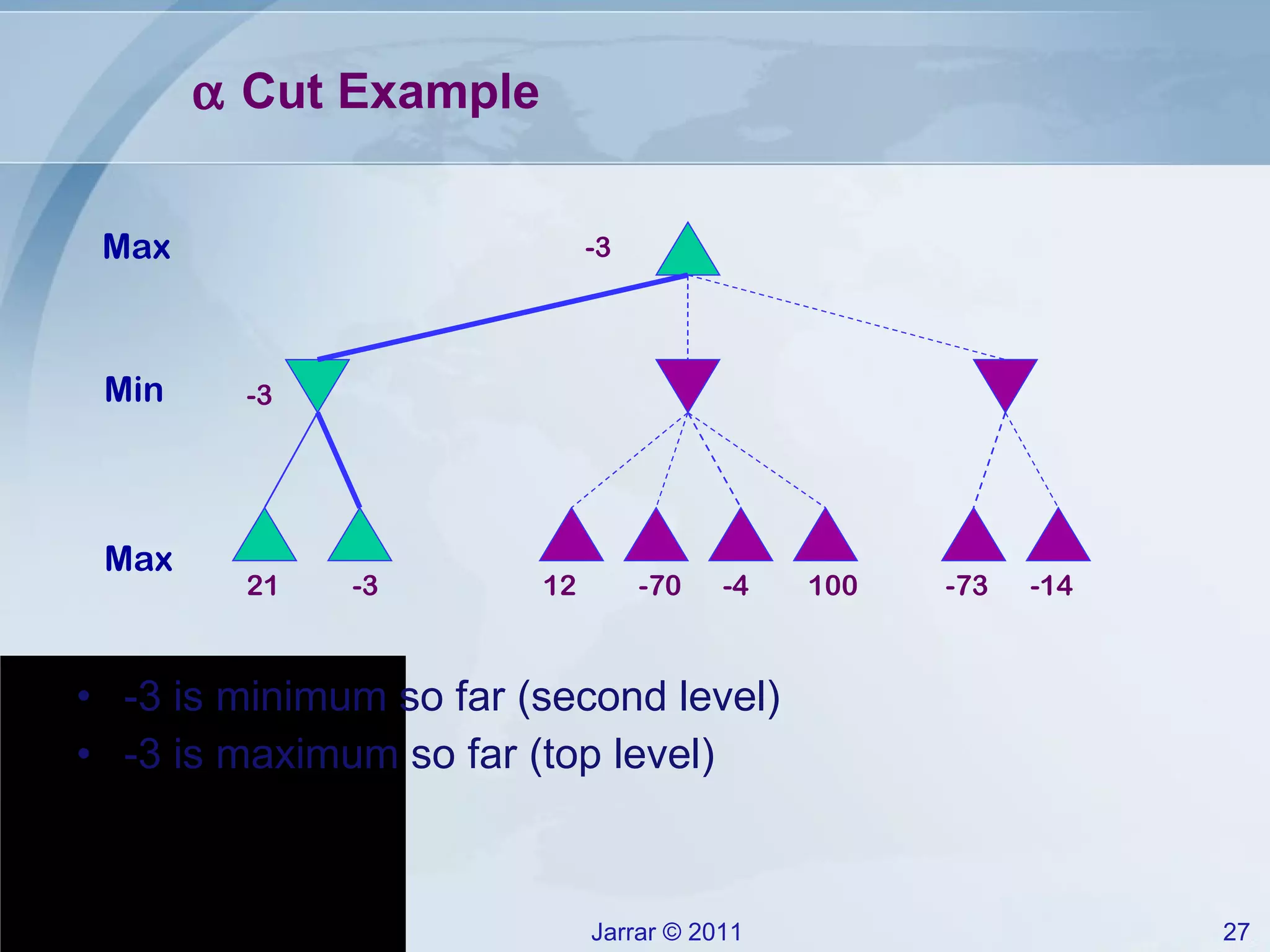
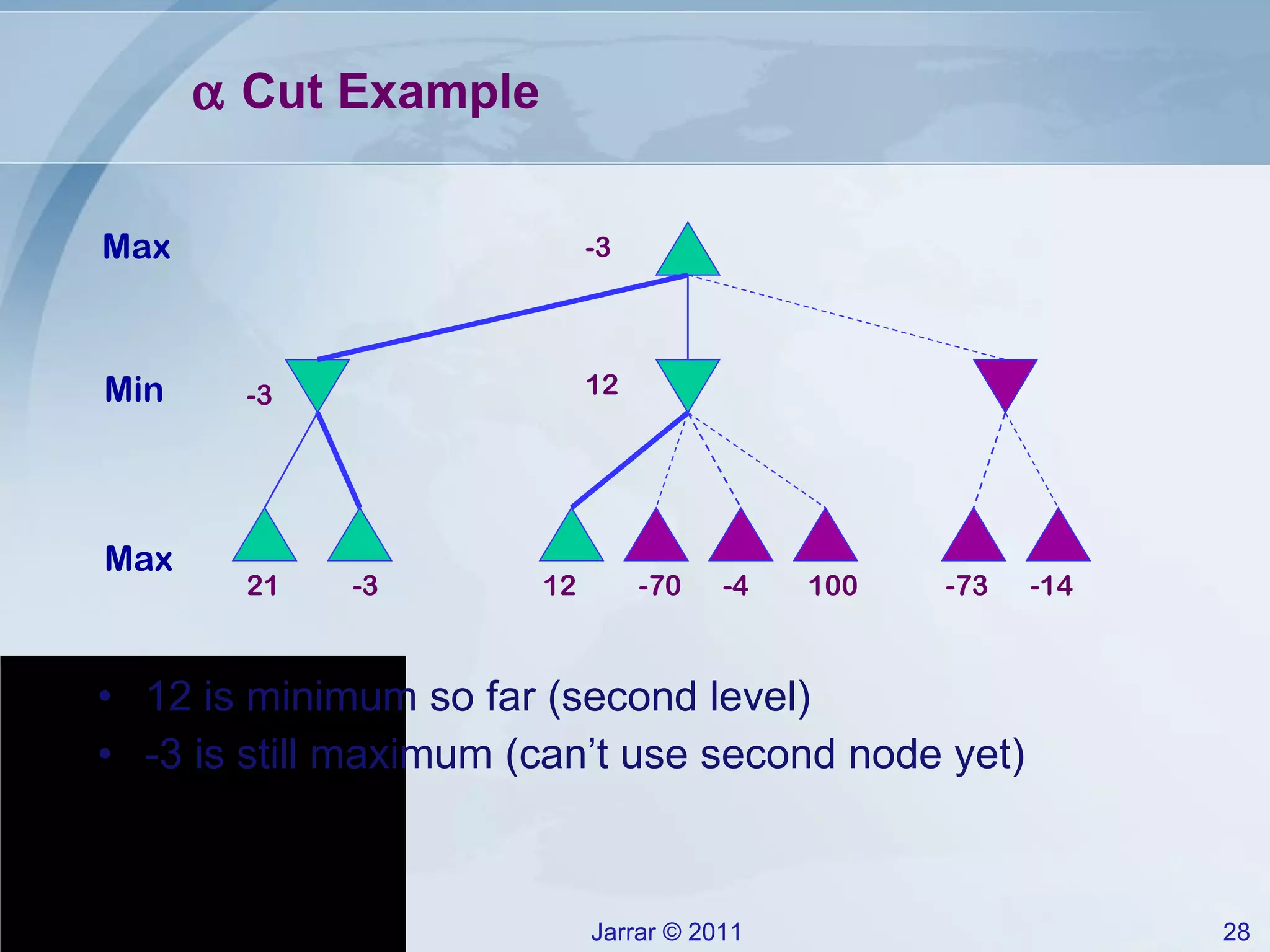
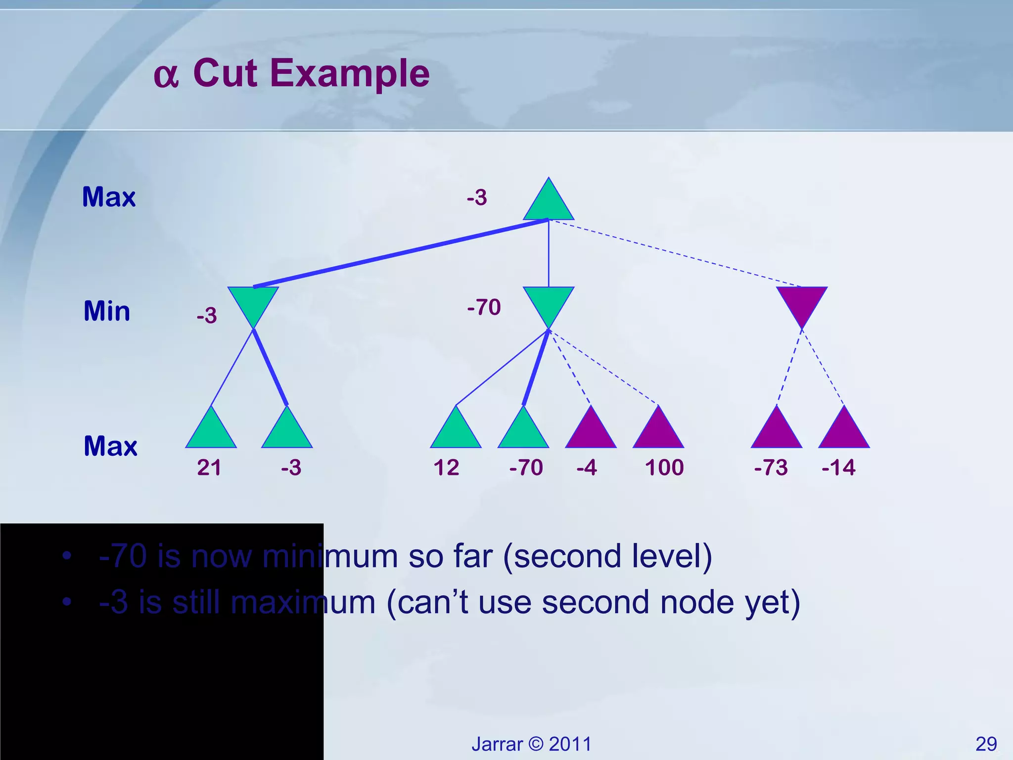
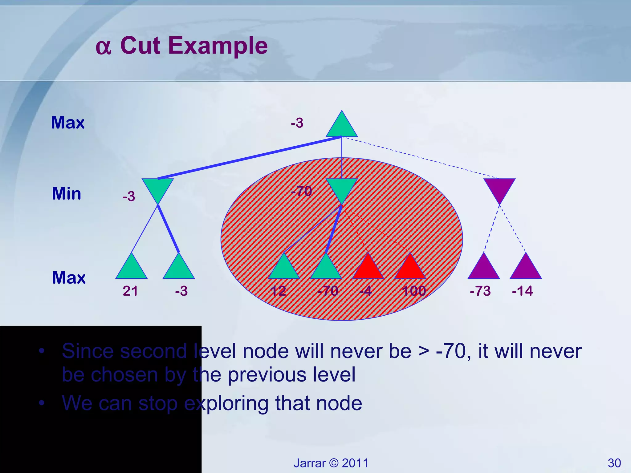
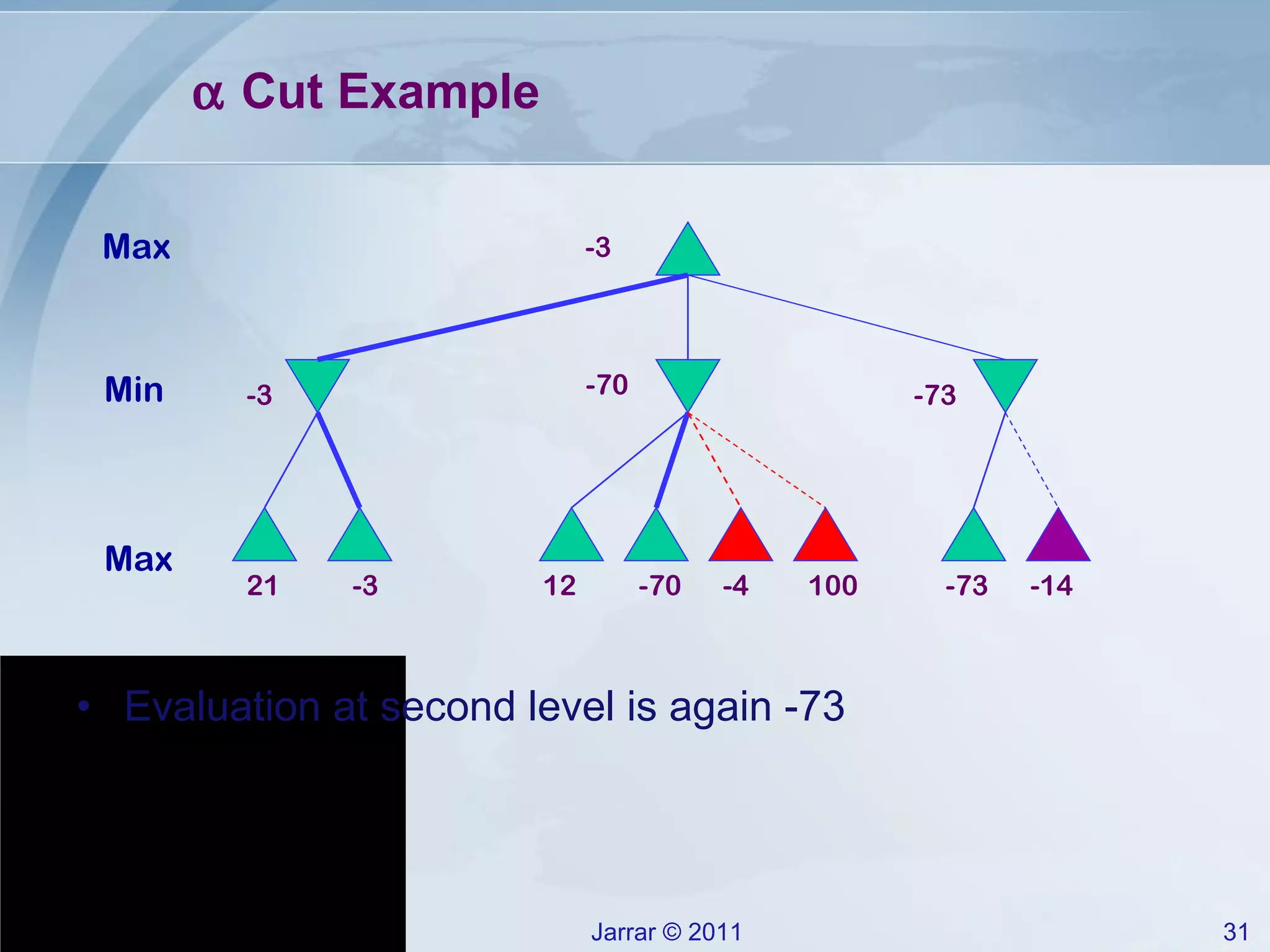
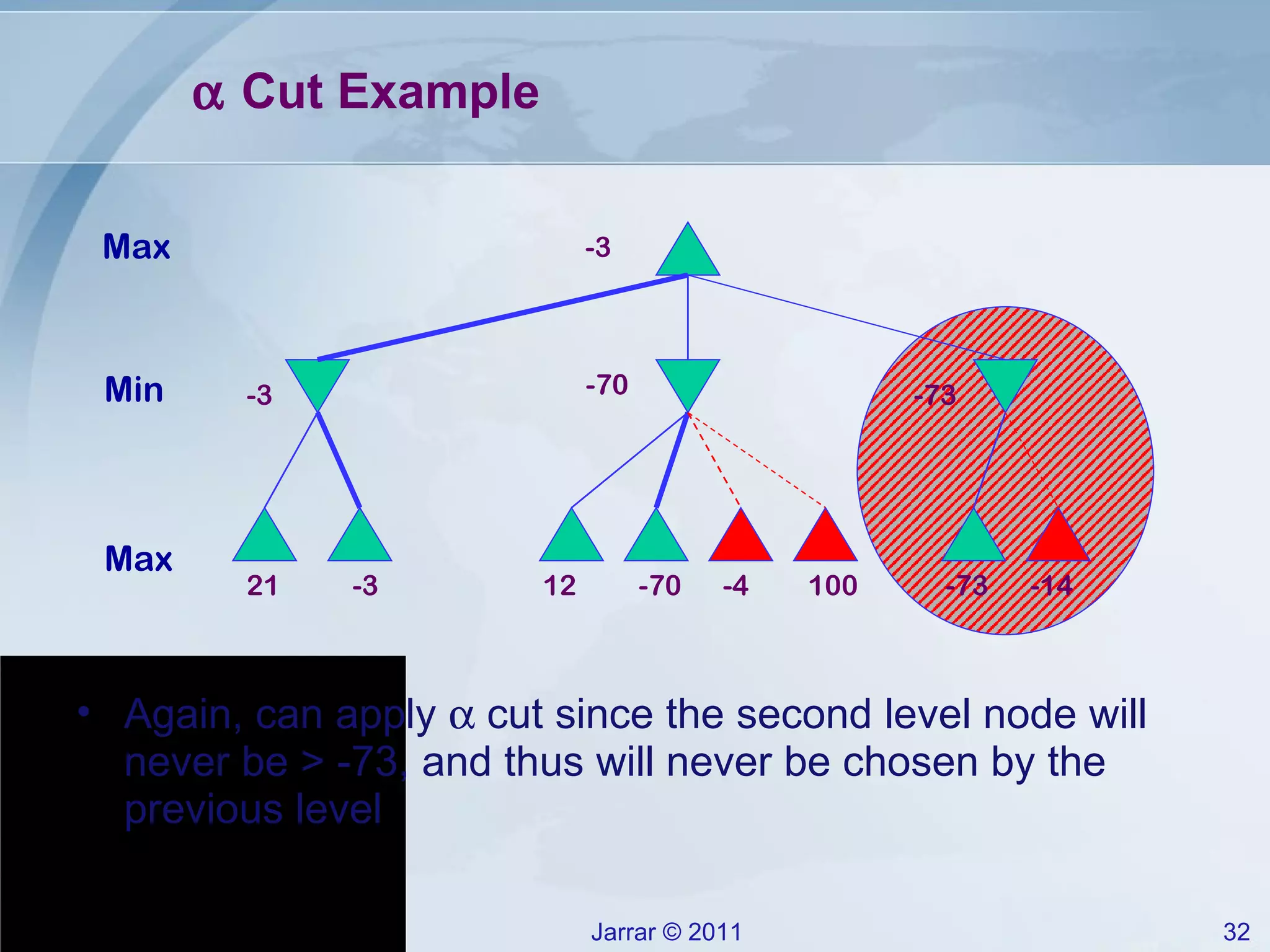
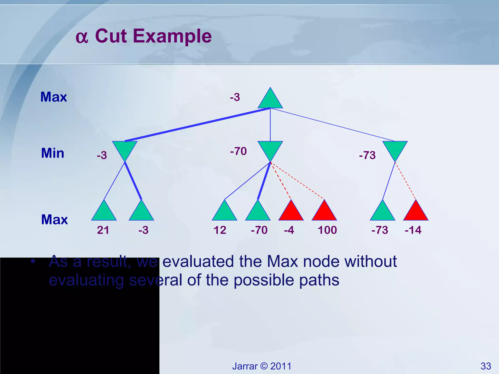
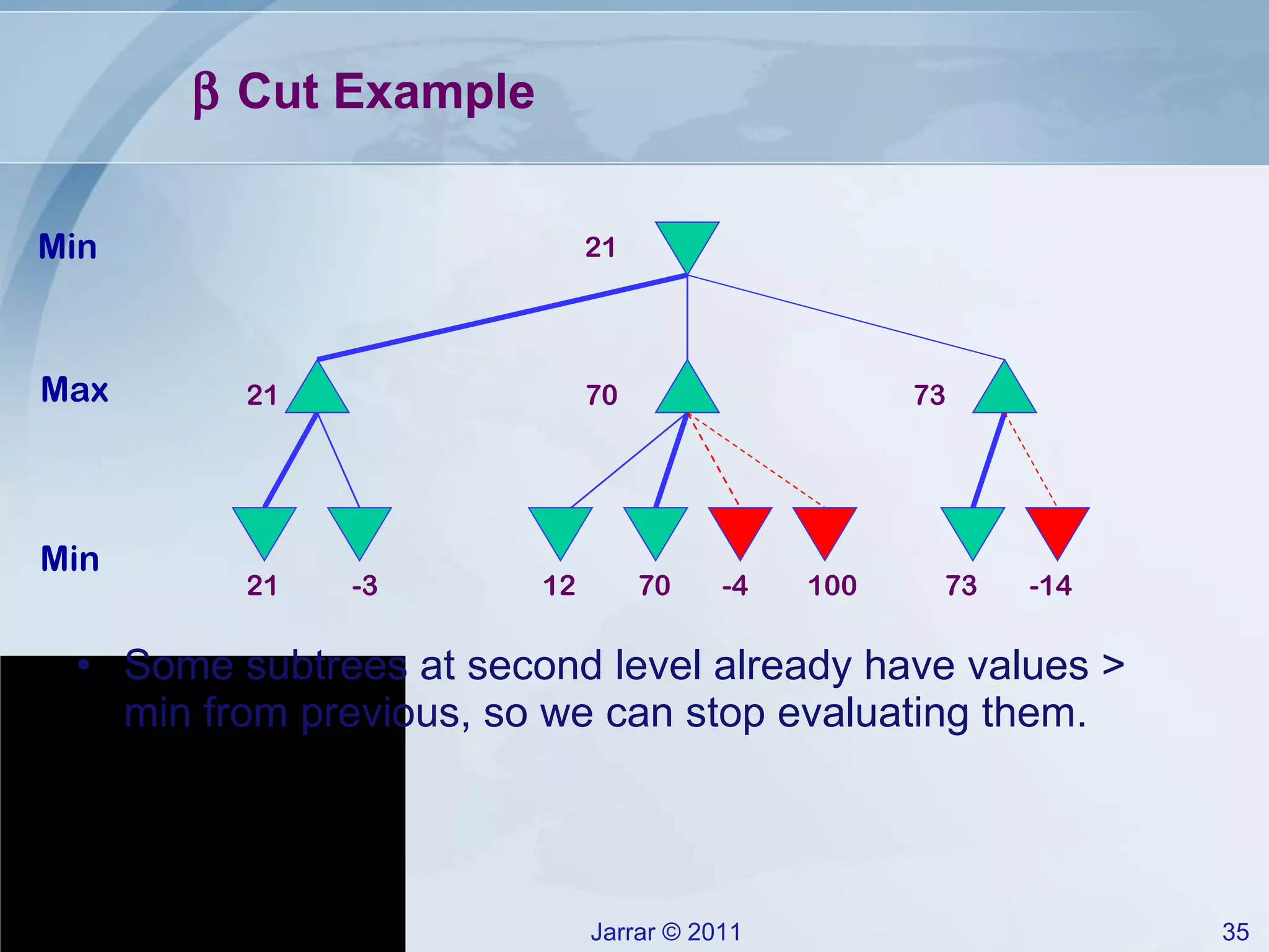
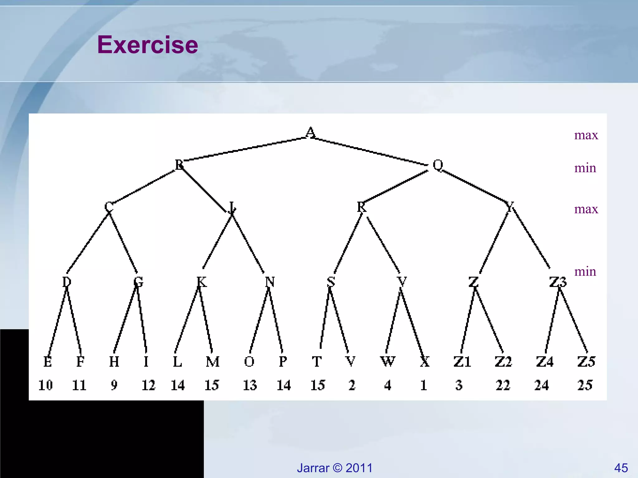
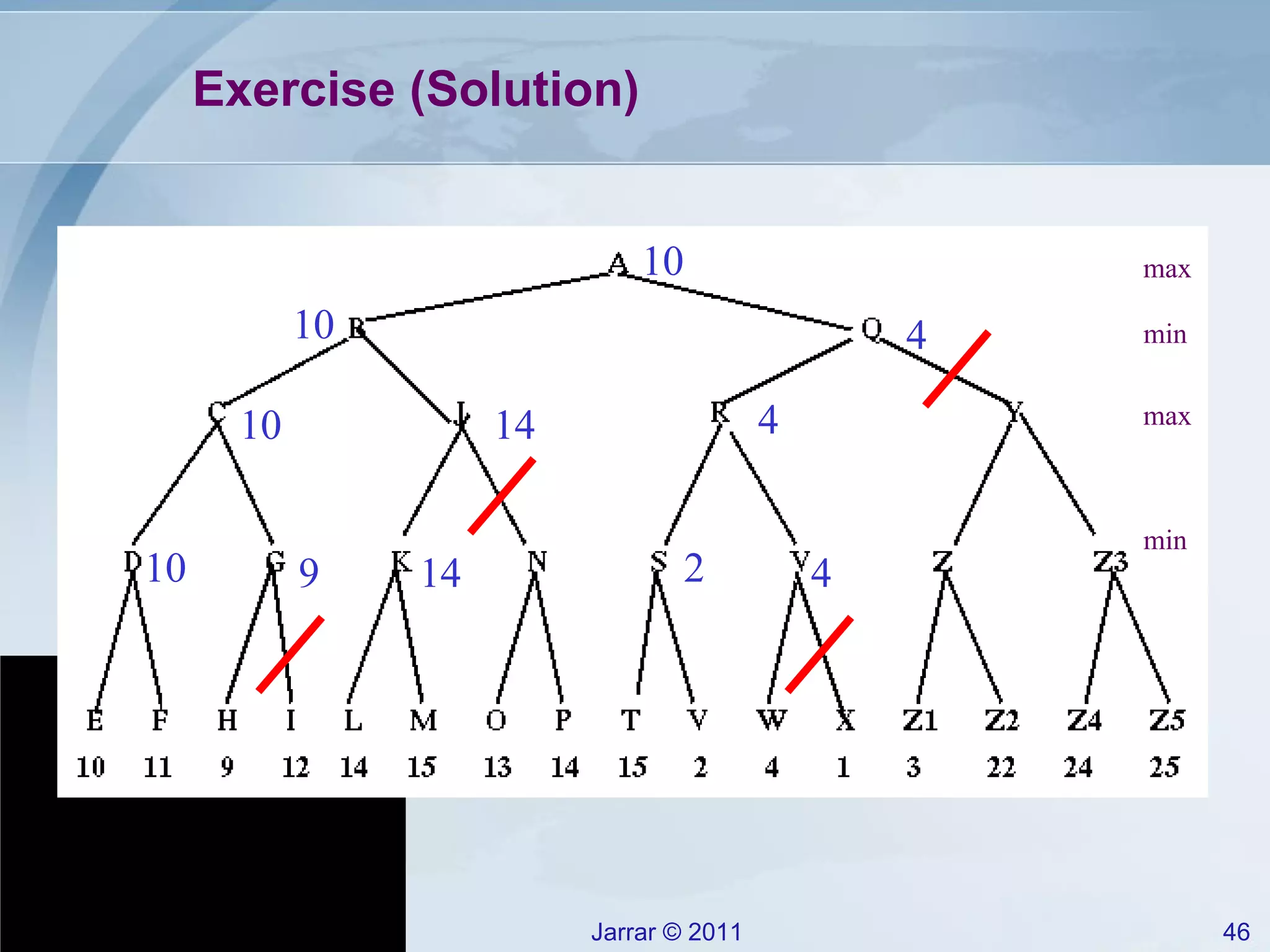
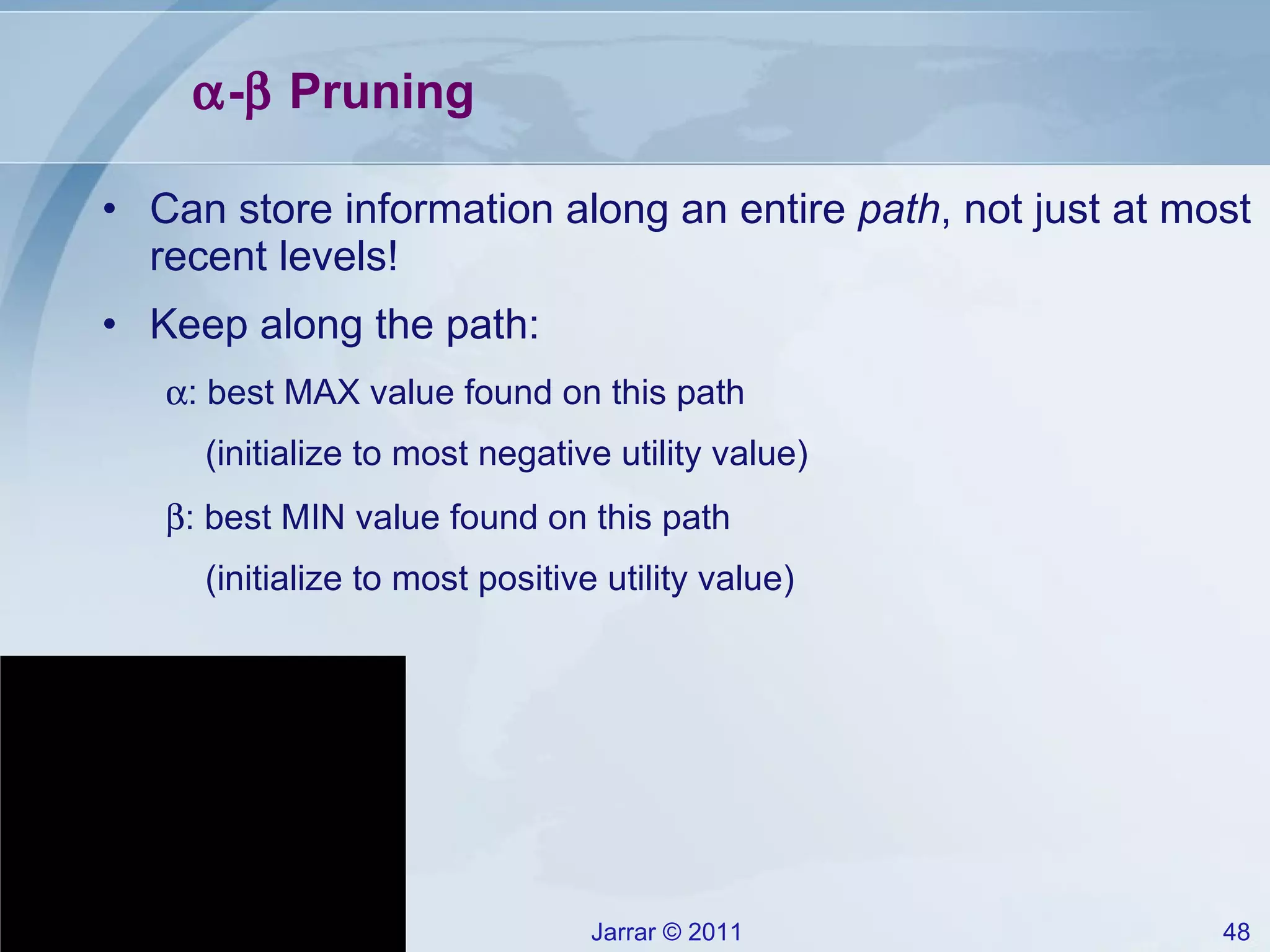
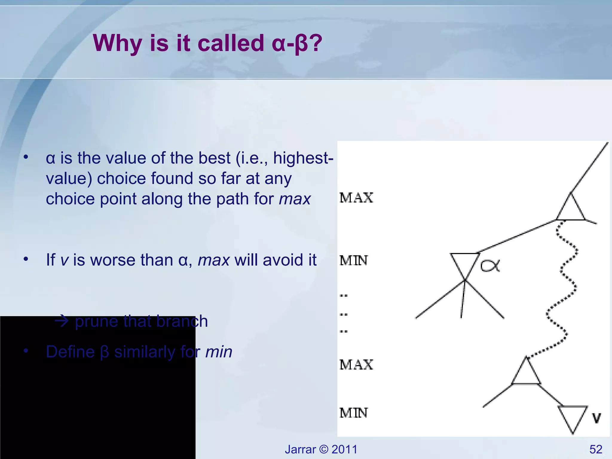
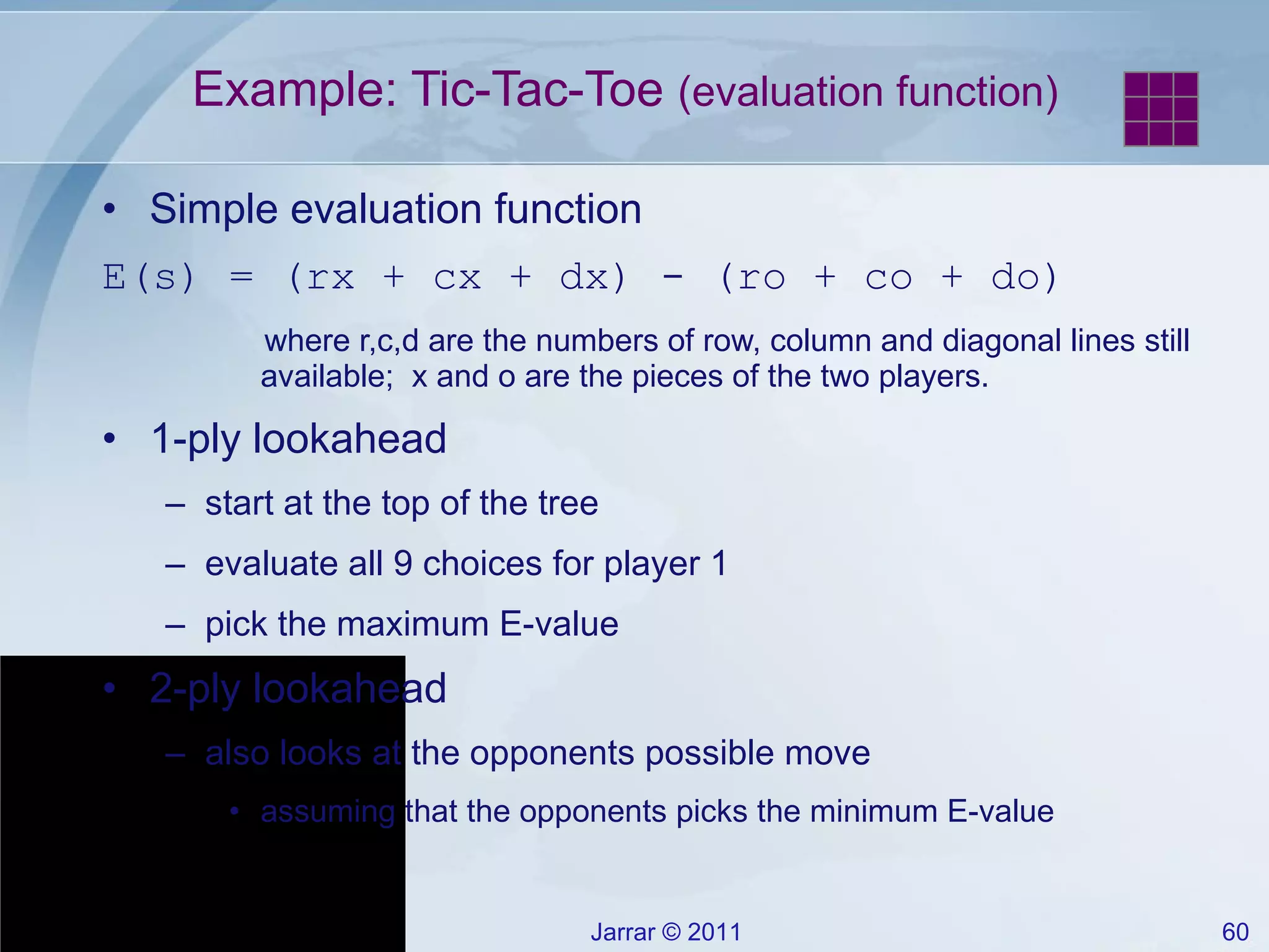
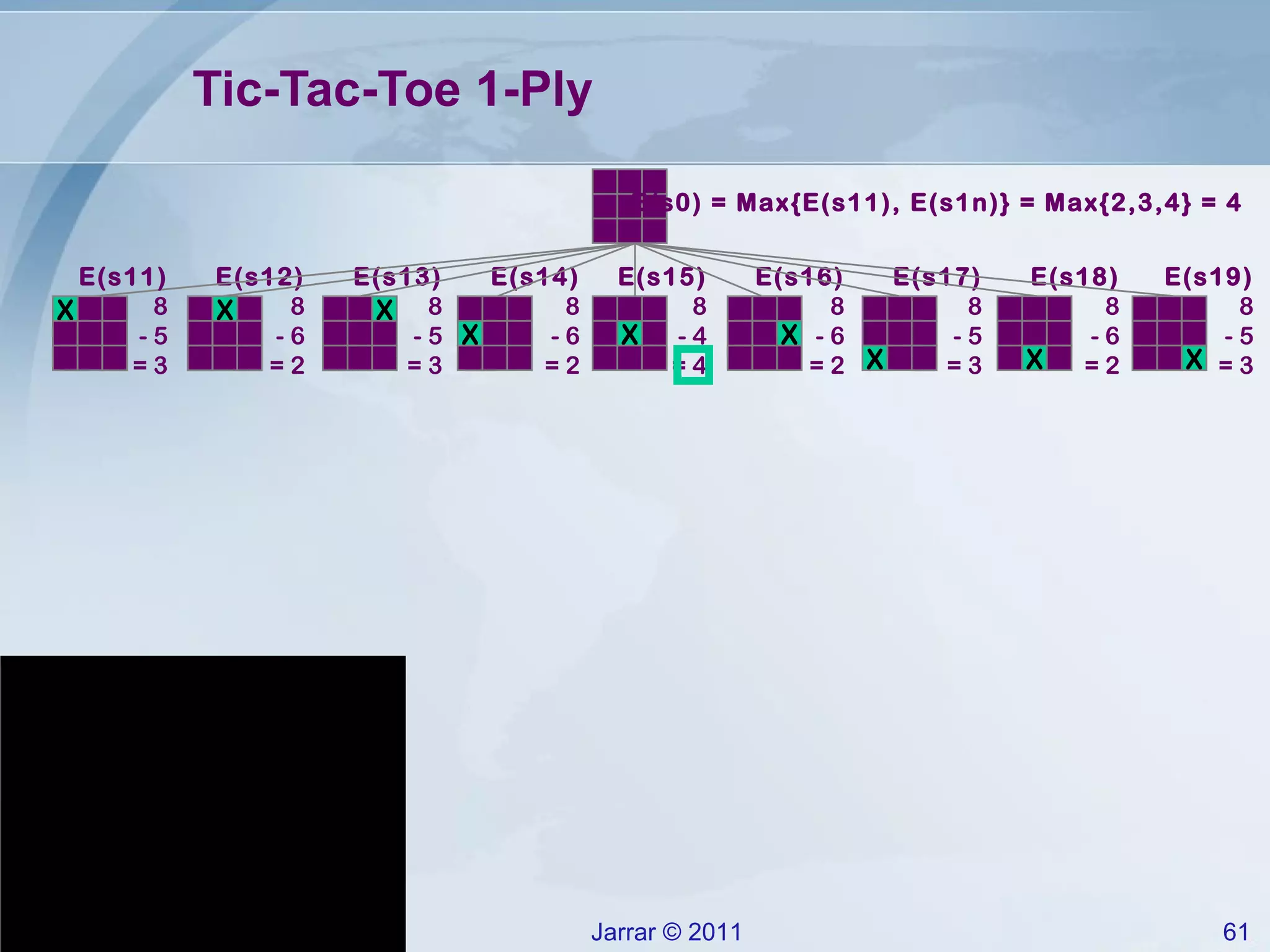
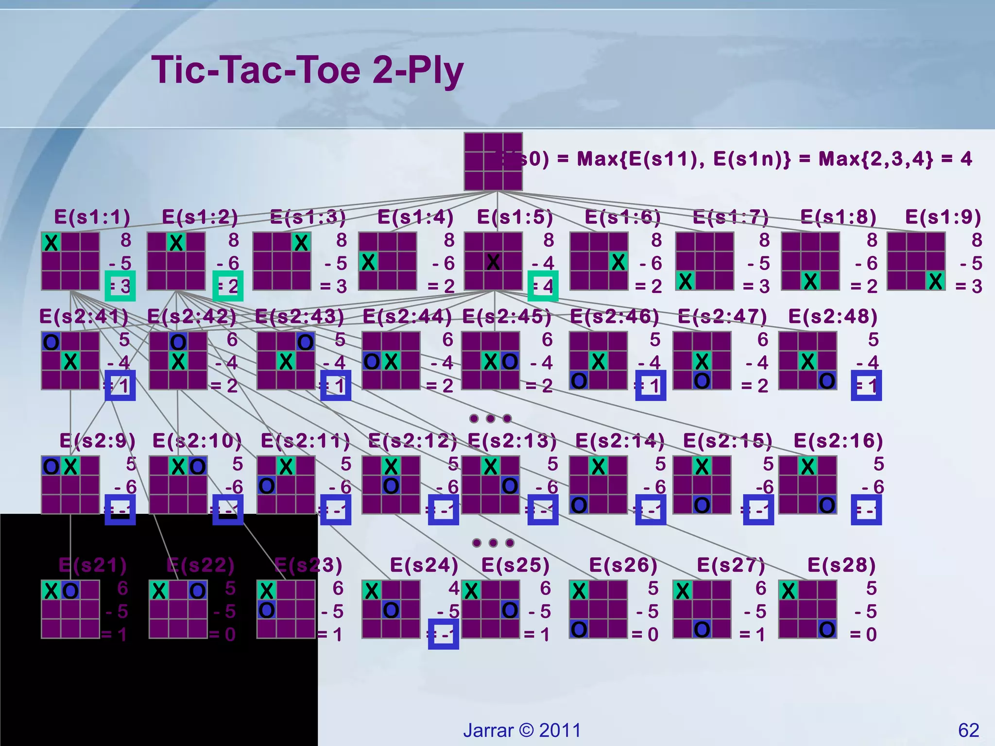
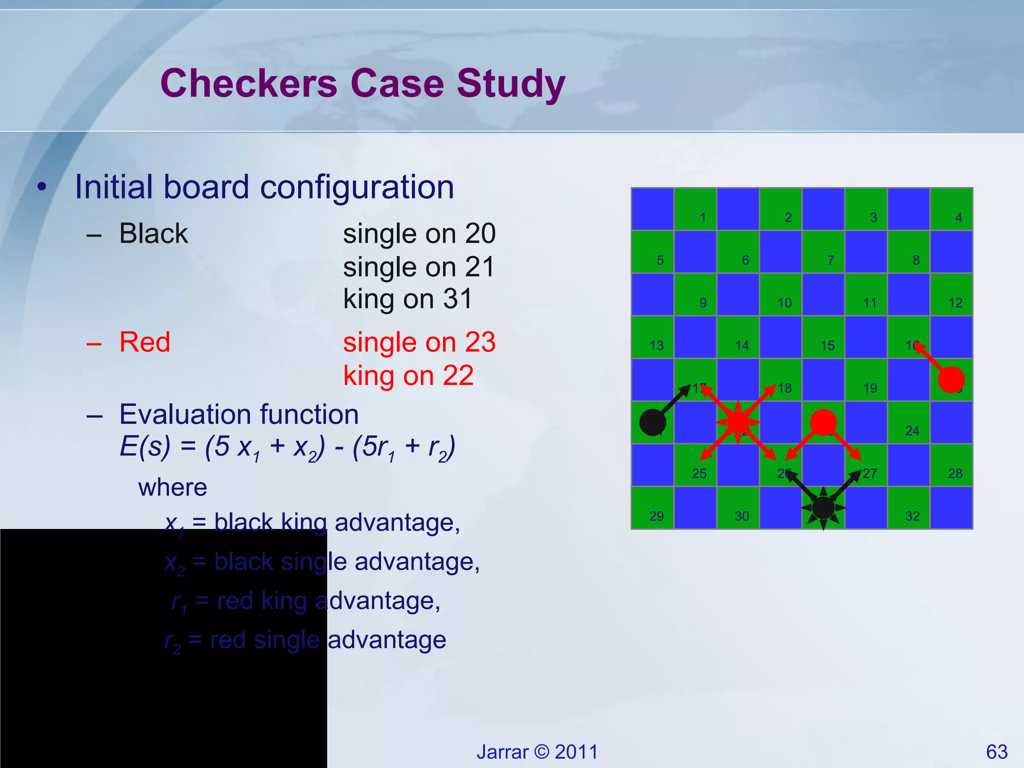
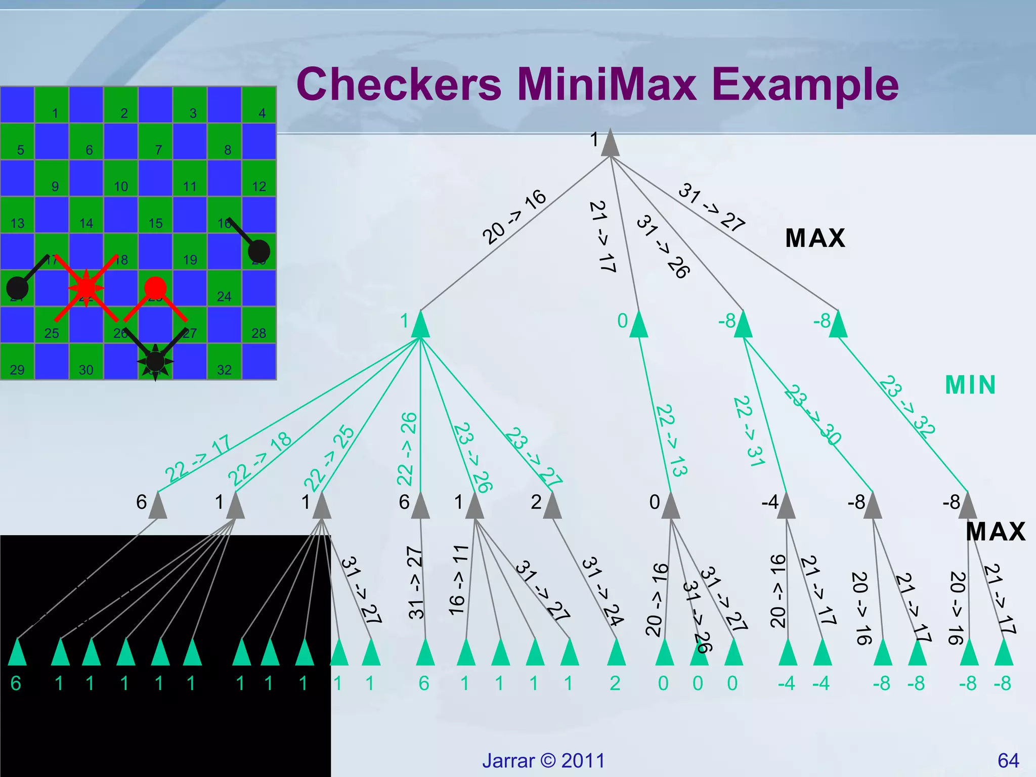
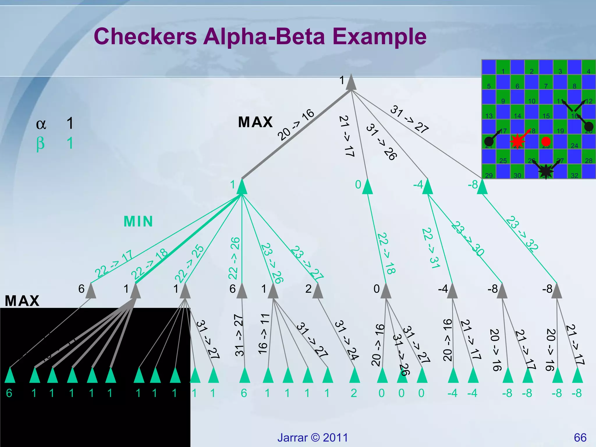
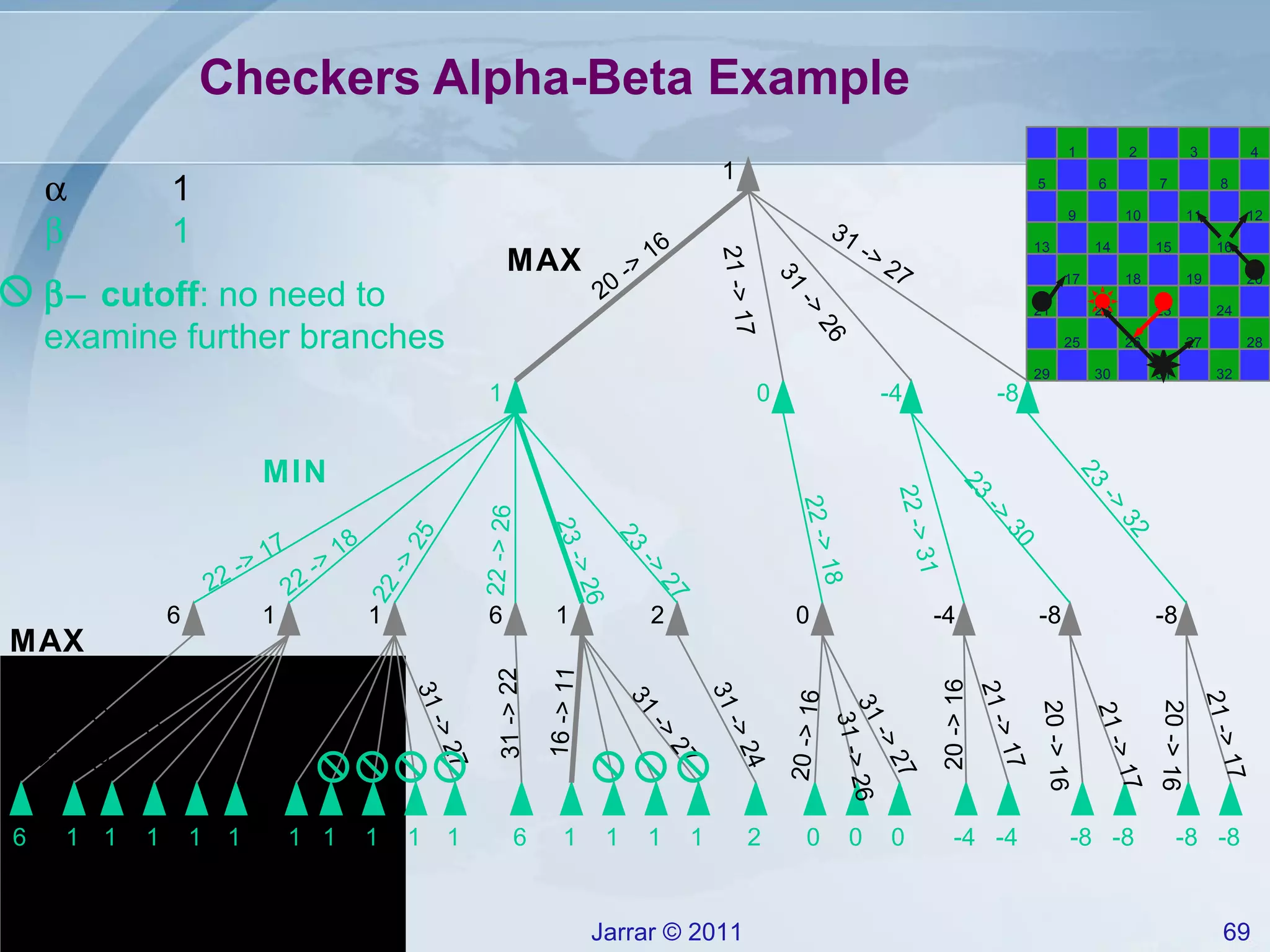
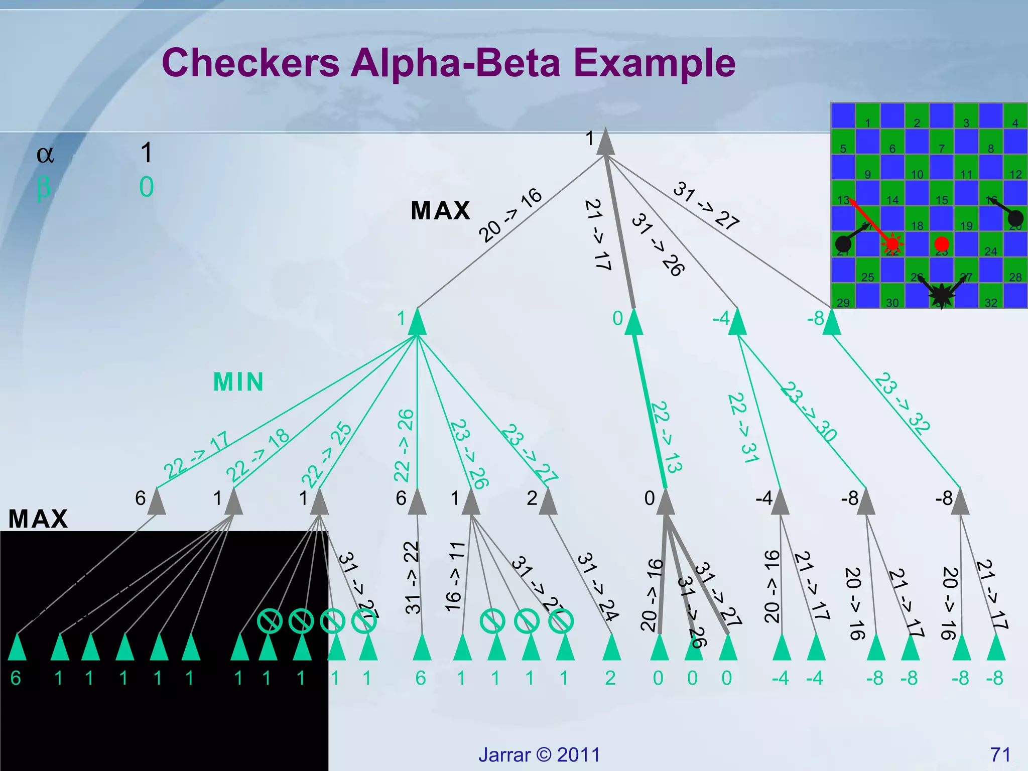
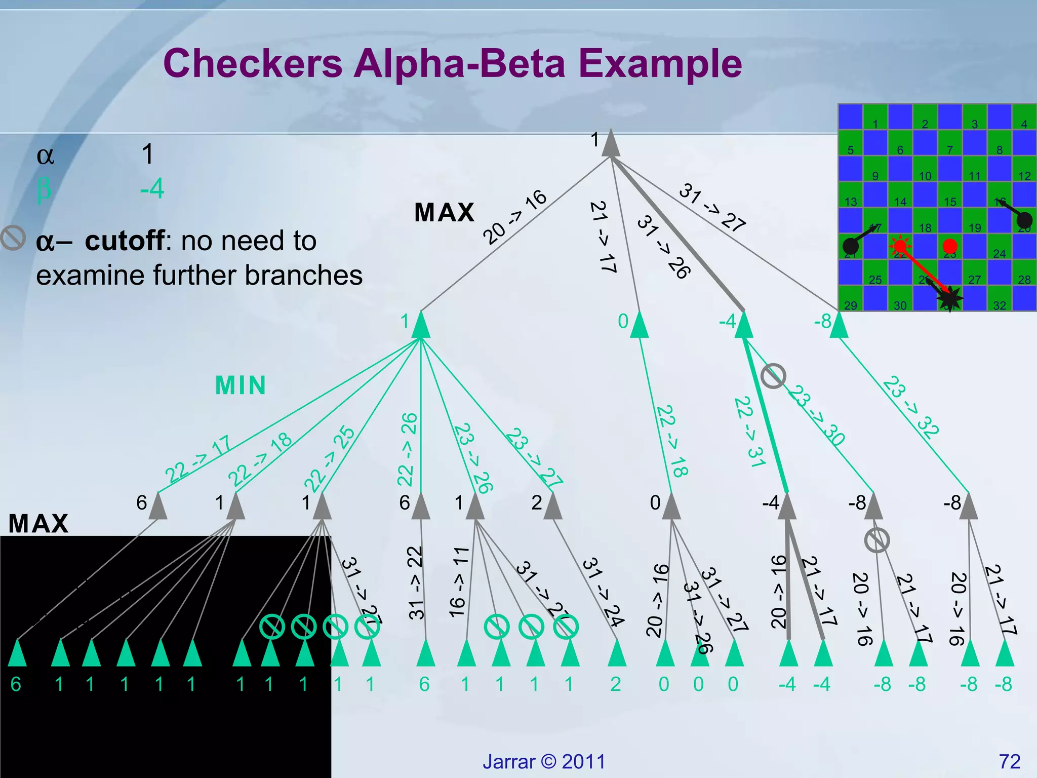
The document discusses game tree search and the minimax algorithm for two-player perfect information games. It introduces the concepts of the minimax tree, terminal node evaluations, and alpha-beta pruning to improve search efficiency. Examples are provided to illustrate how minimax and alpha-beta pruning are applied to search game trees and select the best move.


![SHS_Core_CAE_Q3_LE1 FOR THIRD [FINAL].pdf](https://cdn.slidesharecdn.com/ss_thumbnails/shscorecaeq3le1final-251116055110-e3081055-thumbnail.jpg?width=640&height=640&fit=bounds)


