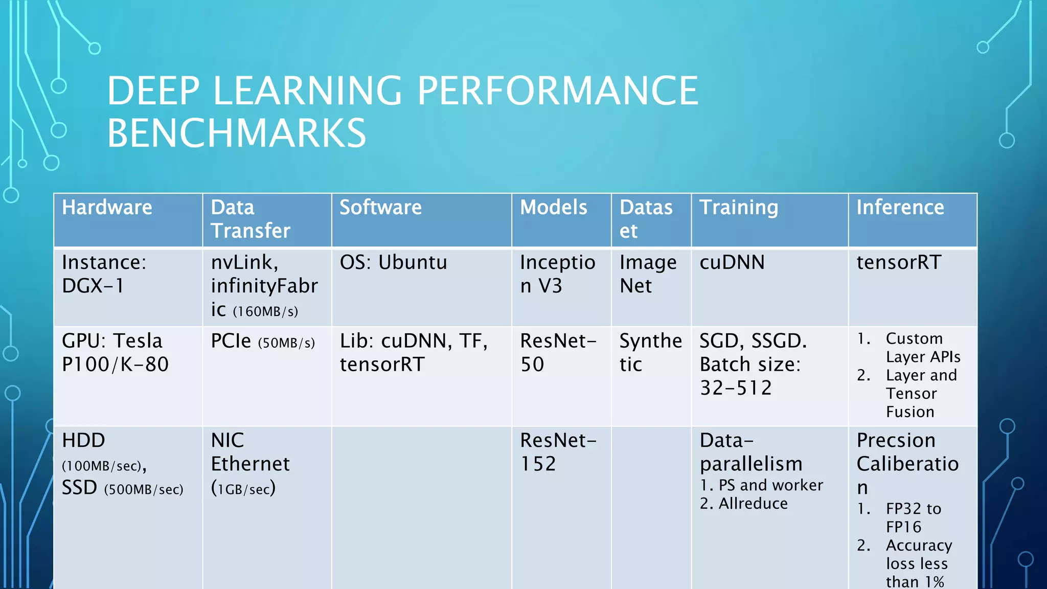
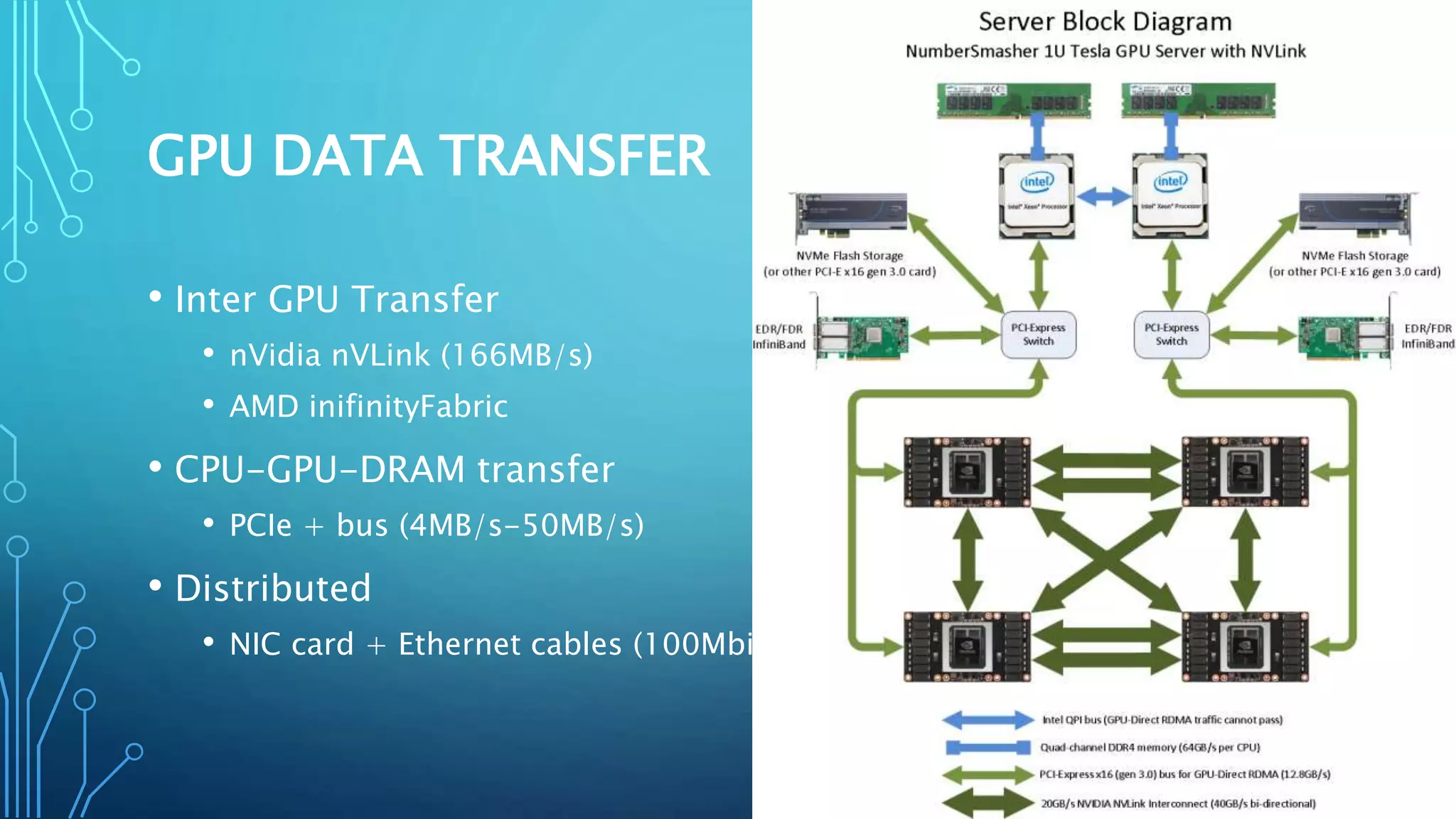
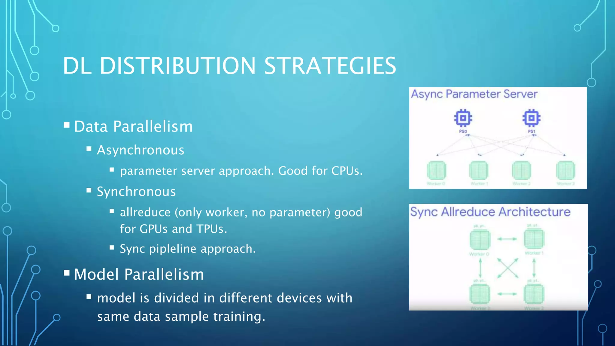
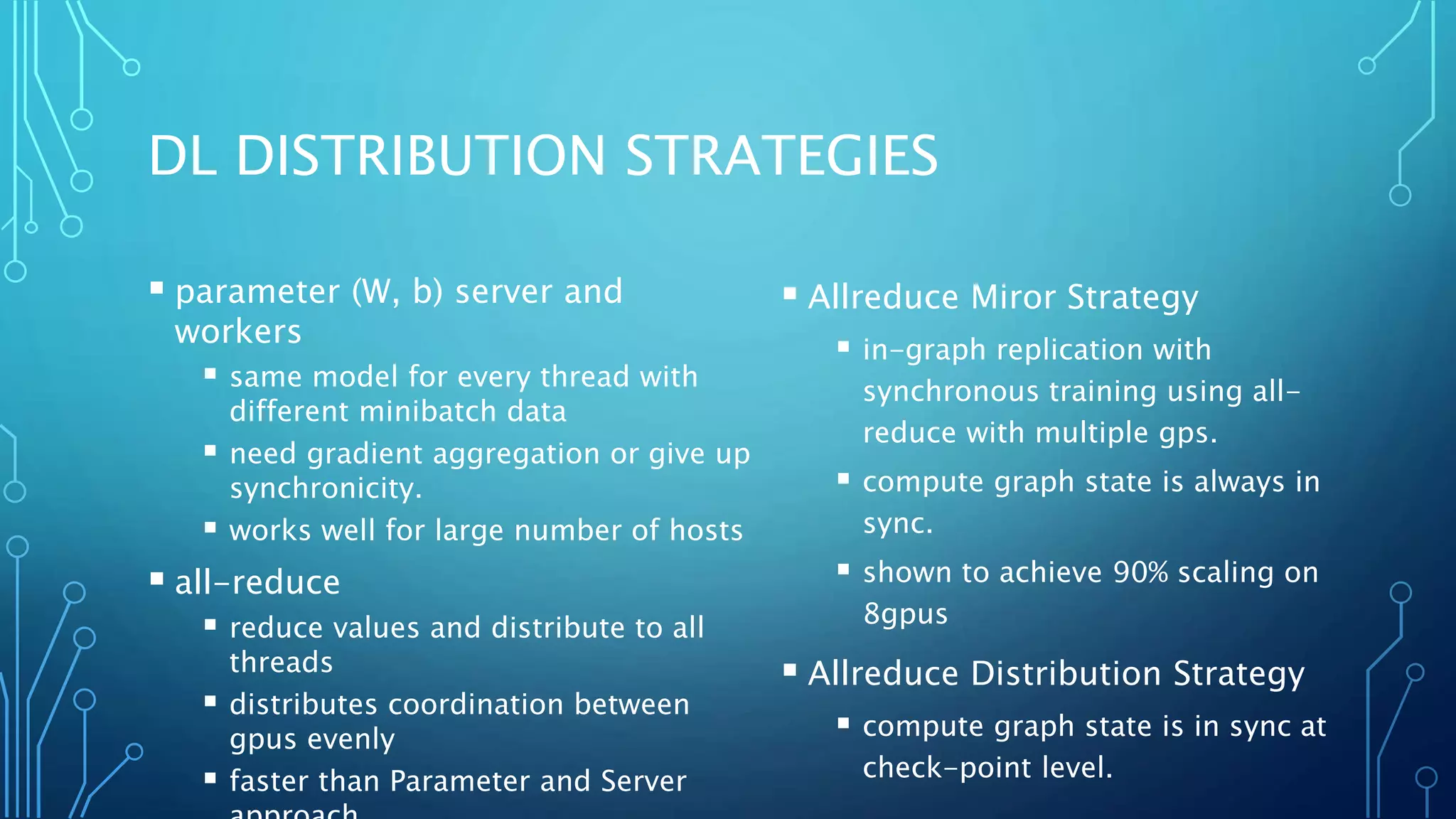
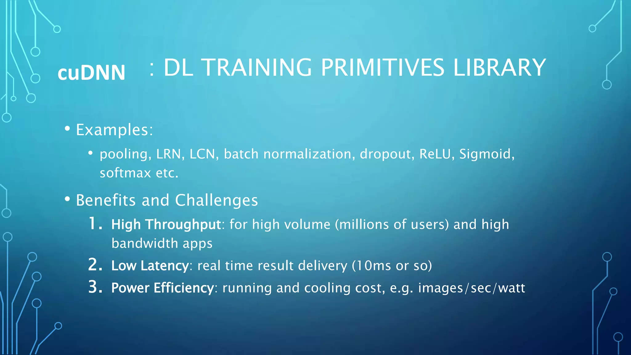
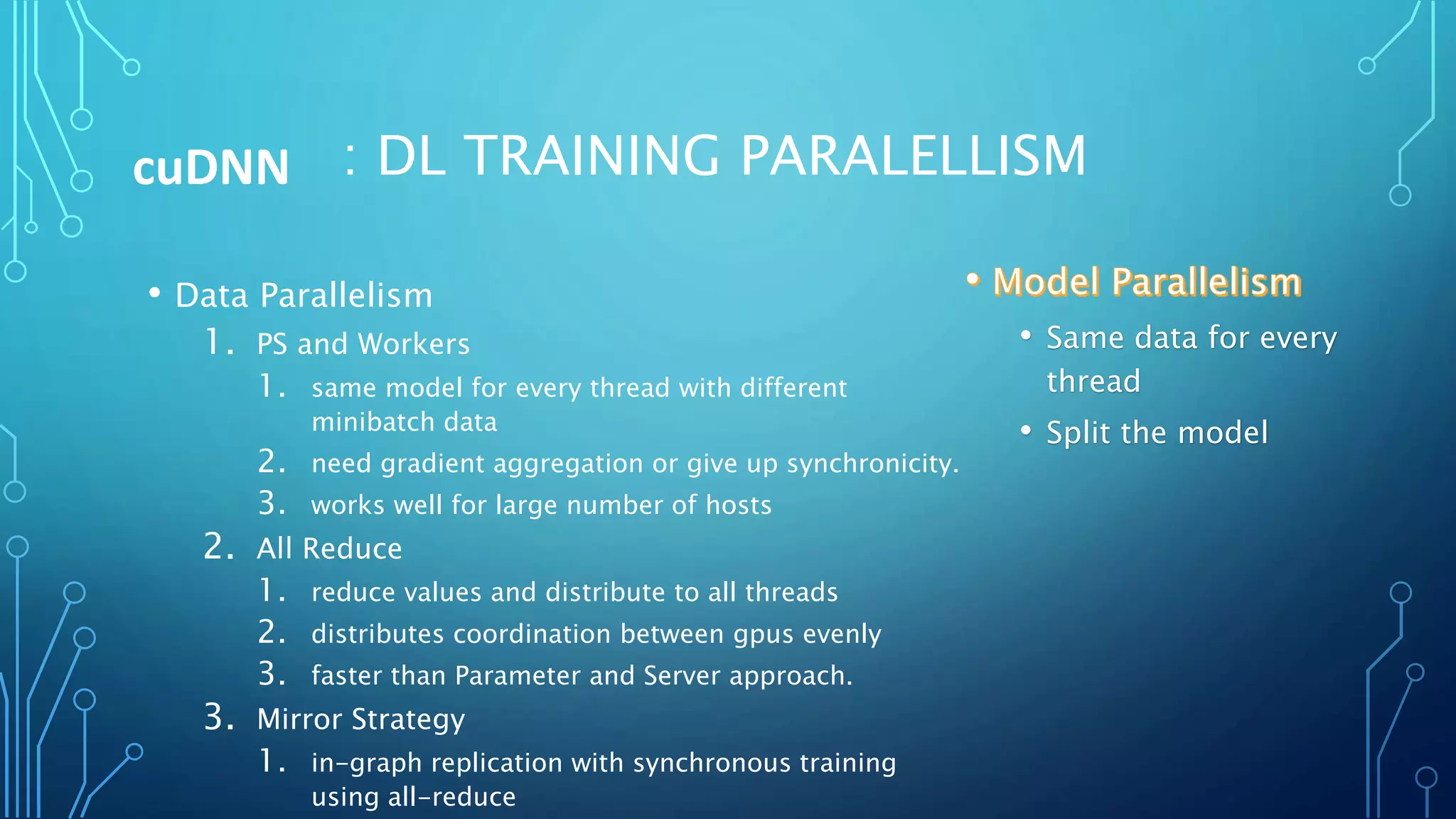
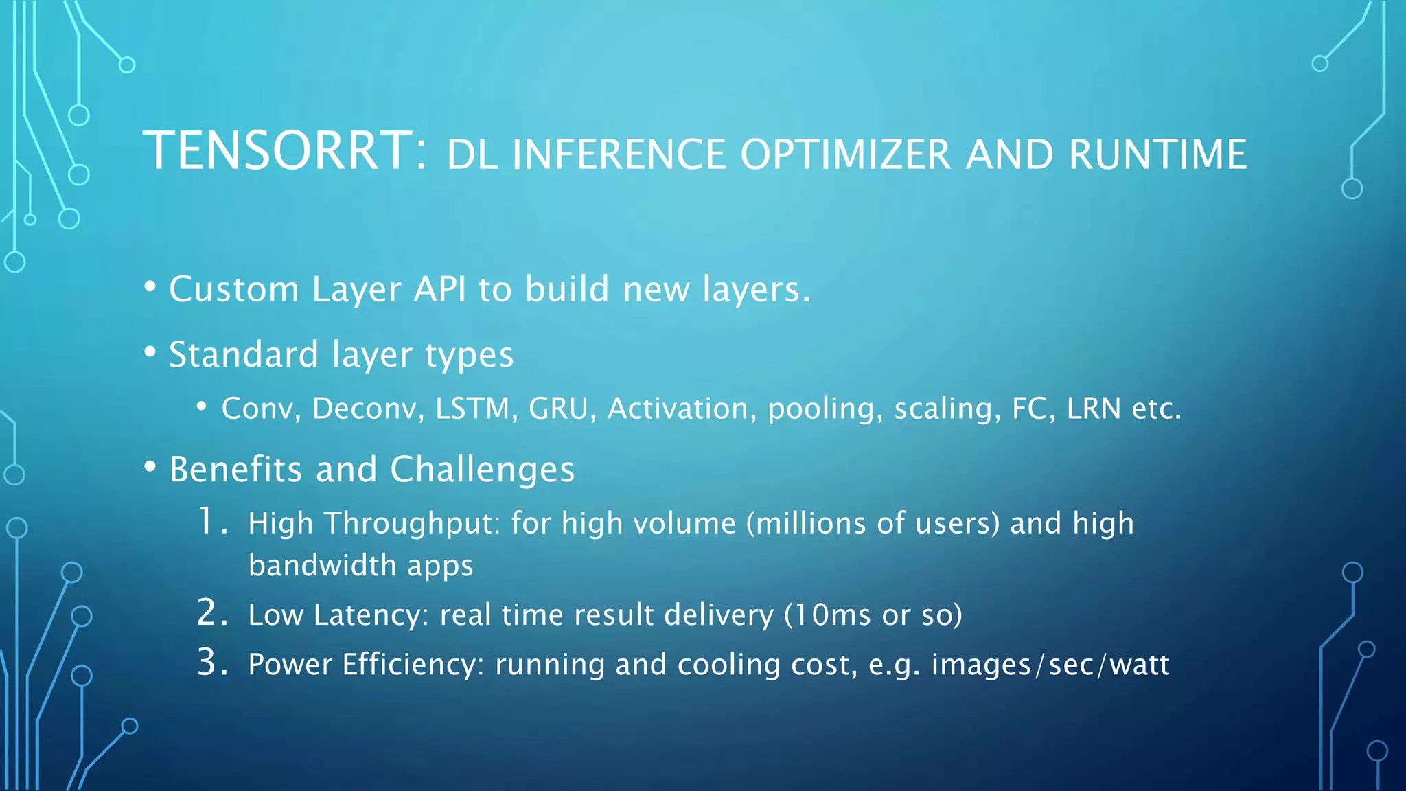
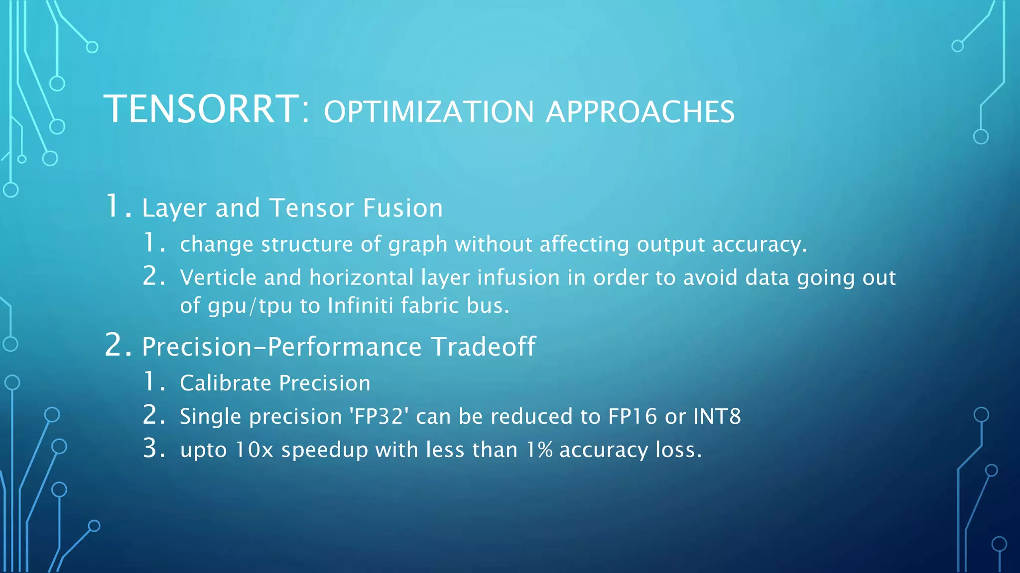
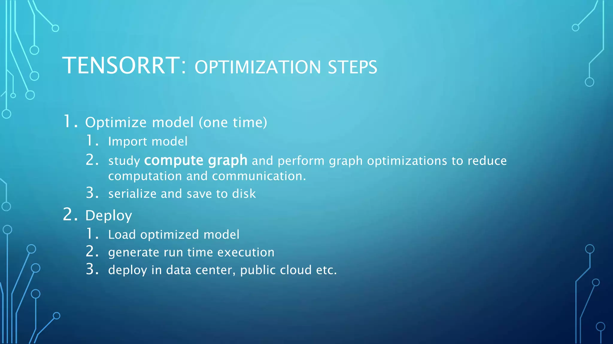
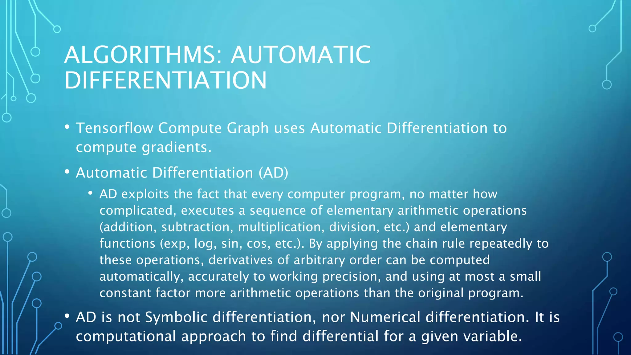
7 POINTS TO PONDER,
BEFORE YOU USE GPUS TO
SPEED UP MACHINE
LEARNING APPS
DEEP LEARNING PERFORMANCE
BENCHMARKS
Hardware Data
Transfer
Software Models Datas
et
Training Inference
Instance:
DGX-1
nvLink,
infinityFabr
ic (160MB/s)
OS: Ubuntu Inceptio
n V3
Image
Net
cuDNN tensorRT
GPU: Tesla
P100/K-80
PCIe (50MB/s) Lib: cuDNN, TF,
tensorRT
ResNet-
50
Synthe
tic
SGD, SSGD.
Batch size:
32-512
1. Custom
Layer APIs
2. Layer and
Tensor
Fusion
HDD
(100MB/sec),
SSD (500MB/sec)
NIC
Ethernet
(1GB/sec)
ResNet-
152
Data-
parallelism
1. PS and worker
2. Allreduce
Precsion
Caliberatio
n
1. FP32 to
FP16
2. Accuracy
loss less
than 1%
HARDWARE
• No. of GPUs in a single instance
• GPU Instance cliques
• Deep Learning Instructions Set
• System memory and GPU memory
GPU DATA TRANSFER
• Inter GPU Transfer
• nVidia nVLink (166MB/s)
• AMD inifinityFabric
• CPU-GPU-DRAM transfer
• PCIe + bus (4MB/s-50MB/s)
• Distributed
• NIC card + Ethernet cables (100Mbits/s)
MODELS AND DATASET
• ImageNet
• Synthetic
PARALLELISM
• Multi Threading
• Multi process
• Distributed
DL: TRAINING DATA PIPELINE
• Data Pipeline
• Extract: disk/nfs/hdfs to physical mem (DRAM)
• Transform: DRAM to CPU
• Load: DRAM to GPU/TPU
• Optimization
• data prefetch on gpu before it is needed
• Standard protocol buffer
DL TRAINING PERFORMANCE TUNING
1. Input pipeline performance.
• Measure performance
• Find bottleneck
• Optimize bottleneck
• Repeat
DL DISTRIBUTION STRATEGIES
Data Parallelism
 Asynchronous
 parameter server approach. Good for CPUs.
 Synchronous
 allreduce (only worker, no parameter) good
for GPUs and TPUs.
 Sync pipleline approach.
Model Parallelism
 model is divided in different devices with
same data sample training.
DL DISTRIBUTION STRATEGIES
 parameter (W, b) server and
workers
 same model for every thread with
different minibatch data
 need gradient aggregation or give up
synchronicity.
 works well for large number of hosts
 all-reduce
 reduce values and distribute to all
threads
 distributes coordination between
gpus evenly
 faster than Parameter and Server
 Allreduce Miror Strategy
 in-graph replication with
synchronous training using all-
reduce with multiple gps.
 compute graph state is always in
sync.
 shown to achieve 90% scaling on
8gpus
 Allreduce Distribution Strategy
 compute graph state is in sync at
check-point level.
: DL TRAINING PRIMITIVES LIBRARY
• Examples:
• pooling, LRN, LCN, batch normalization, dropout, ReLU, Sigmoid,
softmax etc.
• Benefits and Challenges
1. High Throughput: for high volume (millions of users) and high
bandwidth apps
2. Low Latency: real time result delivery (10ms or so)
3. Power Efficiency: running and cooling cost, e.g. images/sec/watt
cuDNN
: DL TRAINING PARALELLISM
• Data Parallelism
1. PS and Workers
1. same model for every thread with different
minibatch data
2. need gradient aggregation or give up synchronicity.
3. works well for large number of hosts
2. All Reduce
1. reduce values and distribute to all threads
2. distributes coordination between gpus evenly
3. faster than Parameter and Server approach.
3. Mirror Strategy
1. in-graph replication with synchronous training
using all-reduce
cuDNN
• Same data for every
thread
• Split the model
TENSORRT: DL INFERENCE OPTIMIZER AND RUNTIME
• Custom Layer API to build new layers.
• Standard layer types
• Conv, Deconv, LSTM, GRU, Activation, pooling, scaling, FC, LRN etc.
• Benefits and Challenges
1. High Throughput: for high volume (millions of users) and high
bandwidth apps
2. Low Latency: real time result delivery (10ms or so)
3. Power Efficiency: running and cooling cost, e.g. images/sec/watt
TENSORRT: OPTIMIZATION APPROACHES
1. Layer and Tensor Fusion
1. change structure of graph without affecting output accuracy.
2. Verticle and horizontal layer infusion in order to avoid data going out
of gpu/tpu to Infiniti fabric bus.
2. Precision-Performance Tradeoff
1. Calibrate Precision
2. Single precision 'FP32' can be reduced to FP16 or INT8
3. upto 10x speedup with less than 1% accuracy loss.
TENSORRT: OPTIMIZATION STEPS
1. Optimize model (one time)
1. Import model
2. study compute graph and perform graph optimizations to reduce
computation and communication.
3. serialize and save to disk
2. Deploy
1. Load optimized model
2. generate run time execution
3. deploy in data center, public cloud etc.
ALGORITHMS: AUTOMATIC
DIFFERENTIATION
• Tensorflow Compute Graph uses Automatic Differentiation to
compute gradients.
• Automatic Differentiation (AD)
• AD exploits the fact that every computer program, no matter how
complicated, executes a sequence of elementary arithmetic operations
(addition, subtraction, multiplication, division, etc.) and elementary
functions (exp, log, sin, cos, etc.). By applying the chain rule repeatedly to
these operations, derivatives of arbitrary order can be computed
automatically, accurately to working precision, and using at most a small
constant factor more arithmetic operations than the original program.
• AD is not Symbolic differentiation, nor Numerical differentiation. It is
computational approach to find differential for a given variable.

improve deep learning training and inference performance

  • 1.
    7 POINTS TOPONDER, BEFORE YOU USE GPUS TO SPEED UP MACHINE LEARNING APPS
  • 2.
    DEEP LEARNING PERFORMANCE BENCHMARKS HardwareData Transfer Software Models Datas et Training Inference Instance: DGX-1 nvLink, infinityFabr ic (160MB/s) OS: Ubuntu Inceptio n V3 Image Net cuDNN tensorRT GPU: Tesla P100/K-80 PCIe (50MB/s) Lib: cuDNN, TF, tensorRT ResNet- 50 Synthe tic SGD, SSGD. Batch size: 32-512 1. Custom Layer APIs 2. Layer and Tensor Fusion HDD (100MB/sec), SSD (500MB/sec) NIC Ethernet (1GB/sec) ResNet- 152 Data- parallelism 1. PS and worker 2. Allreduce Precsion Caliberatio n 1. FP32 to FP16 2. Accuracy loss less than 1%
  • 3.
    HARDWARE • No. ofGPUs in a single instance • GPU Instance cliques • Deep Learning Instructions Set • System memory and GPU memory
  • 4.
    GPU DATA TRANSFER •Inter GPU Transfer • nVidia nVLink (166MB/s) • AMD inifinityFabric • CPU-GPU-DRAM transfer • PCIe + bus (4MB/s-50MB/s) • Distributed • NIC card + Ethernet cables (100Mbits/s)
  • 5.
    MODELS AND DATASET •ImageNet • Synthetic
  • 6.
    PARALLELISM • Multi Threading •Multi process • Distributed
  • 7.
    DL: TRAINING DATAPIPELINE • Data Pipeline • Extract: disk/nfs/hdfs to physical mem (DRAM) • Transform: DRAM to CPU • Load: DRAM to GPU/TPU • Optimization • data prefetch on gpu before it is needed • Standard protocol buffer
  • 8.
    DL TRAINING PERFORMANCETUNING 1. Input pipeline performance. • Measure performance • Find bottleneck • Optimize bottleneck • Repeat
  • 9.
    DL DISTRIBUTION STRATEGIES DataParallelism  Asynchronous  parameter server approach. Good for CPUs.  Synchronous  allreduce (only worker, no parameter) good for GPUs and TPUs.  Sync pipleline approach. Model Parallelism  model is divided in different devices with same data sample training.
  • 10.
    DL DISTRIBUTION STRATEGIES parameter (W, b) server and workers  same model for every thread with different minibatch data  need gradient aggregation or give up synchronicity.  works well for large number of hosts  all-reduce  reduce values and distribute to all threads  distributes coordination between gpus evenly  faster than Parameter and Server  Allreduce Miror Strategy  in-graph replication with synchronous training using all- reduce with multiple gps.  compute graph state is always in sync.  shown to achieve 90% scaling on 8gpus  Allreduce Distribution Strategy  compute graph state is in sync at check-point level.
  • 11.
    : DL TRAININGPRIMITIVES LIBRARY • Examples: • pooling, LRN, LCN, batch normalization, dropout, ReLU, Sigmoid, softmax etc. • Benefits and Challenges 1. High Throughput: for high volume (millions of users) and high bandwidth apps 2. Low Latency: real time result delivery (10ms or so) 3. Power Efficiency: running and cooling cost, e.g. images/sec/watt cuDNN
  • 12.
    : DL TRAININGPARALELLISM • Data Parallelism 1. PS and Workers 1. same model for every thread with different minibatch data 2. need gradient aggregation or give up synchronicity. 3. works well for large number of hosts 2. All Reduce 1. reduce values and distribute to all threads 2. distributes coordination between gpus evenly 3. faster than Parameter and Server approach. 3. Mirror Strategy 1. in-graph replication with synchronous training using all-reduce cuDNN • Same data for every thread • Split the model
  • 13.
    TENSORRT: DL INFERENCEOPTIMIZER AND RUNTIME • Custom Layer API to build new layers. • Standard layer types • Conv, Deconv, LSTM, GRU, Activation, pooling, scaling, FC, LRN etc. • Benefits and Challenges 1. High Throughput: for high volume (millions of users) and high bandwidth apps 2. Low Latency: real time result delivery (10ms or so) 3. Power Efficiency: running and cooling cost, e.g. images/sec/watt
  • 14.
    TENSORRT: OPTIMIZATION APPROACHES 1.Layer and Tensor Fusion 1. change structure of graph without affecting output accuracy. 2. Verticle and horizontal layer infusion in order to avoid data going out of gpu/tpu to Infiniti fabric bus. 2. Precision-Performance Tradeoff 1. Calibrate Precision 2. Single precision 'FP32' can be reduced to FP16 or INT8 3. upto 10x speedup with less than 1% accuracy loss.
  • 15.
    TENSORRT: OPTIMIZATION STEPS 1.Optimize model (one time) 1. Import model 2. study compute graph and perform graph optimizations to reduce computation and communication. 3. serialize and save to disk 2. Deploy 1. Load optimized model 2. generate run time execution 3. deploy in data center, public cloud etc.
  • 16.
    ALGORITHMS: AUTOMATIC DIFFERENTIATION • TensorflowCompute Graph uses Automatic Differentiation to compute gradients. • Automatic Differentiation (AD) • AD exploits the fact that every computer program, no matter how complicated, executes a sequence of elementary arithmetic operations (addition, subtraction, multiplication, division, etc.) and elementary functions (exp, log, sin, cos, etc.). By applying the chain rule repeatedly to these operations, derivatives of arbitrary order can be computed automatically, accurately to working precision, and using at most a small constant factor more arithmetic operations than the original program. • AD is not Symbolic differentiation, nor Numerical differentiation. It is computational approach to find differential for a given variable.