• Pattern
• Patternrecognition system
• Various applications
• Machine Perception
Topics:
3.
What is Pattern?
•A pattern is a regularity in the world or in abstract notions.
• A pattern is
⮚either a physical object, for example a book or a tree or
⮚an abstract notion, like style of talking, or style of writing.
⮚also a shared property of a set of objects; for example, chairs,
rectangles, or blue colored objects
• Pattern gives the description of the object or the notion.
• The description is given in the form of attributes of the object.
• These are also called the features of the object.
4.
What is PatternRecognition?
• Pattern recognition is a data analysis method that uses machine learning
algorithms to automatically recognize patterns and regularities in data.
• This data can be anything from text and images to sounds or other definable
qualities.
• Pattern recognition is a process of finding regularities and similarities in data
using machine learning data.
• Now, these similarities can be found based on statistical analysis, historical
data, or the already gained knowledge by the machine itself.
• Pattern recognition systems can recognize familiar patterns quickly and
accurately.
5.
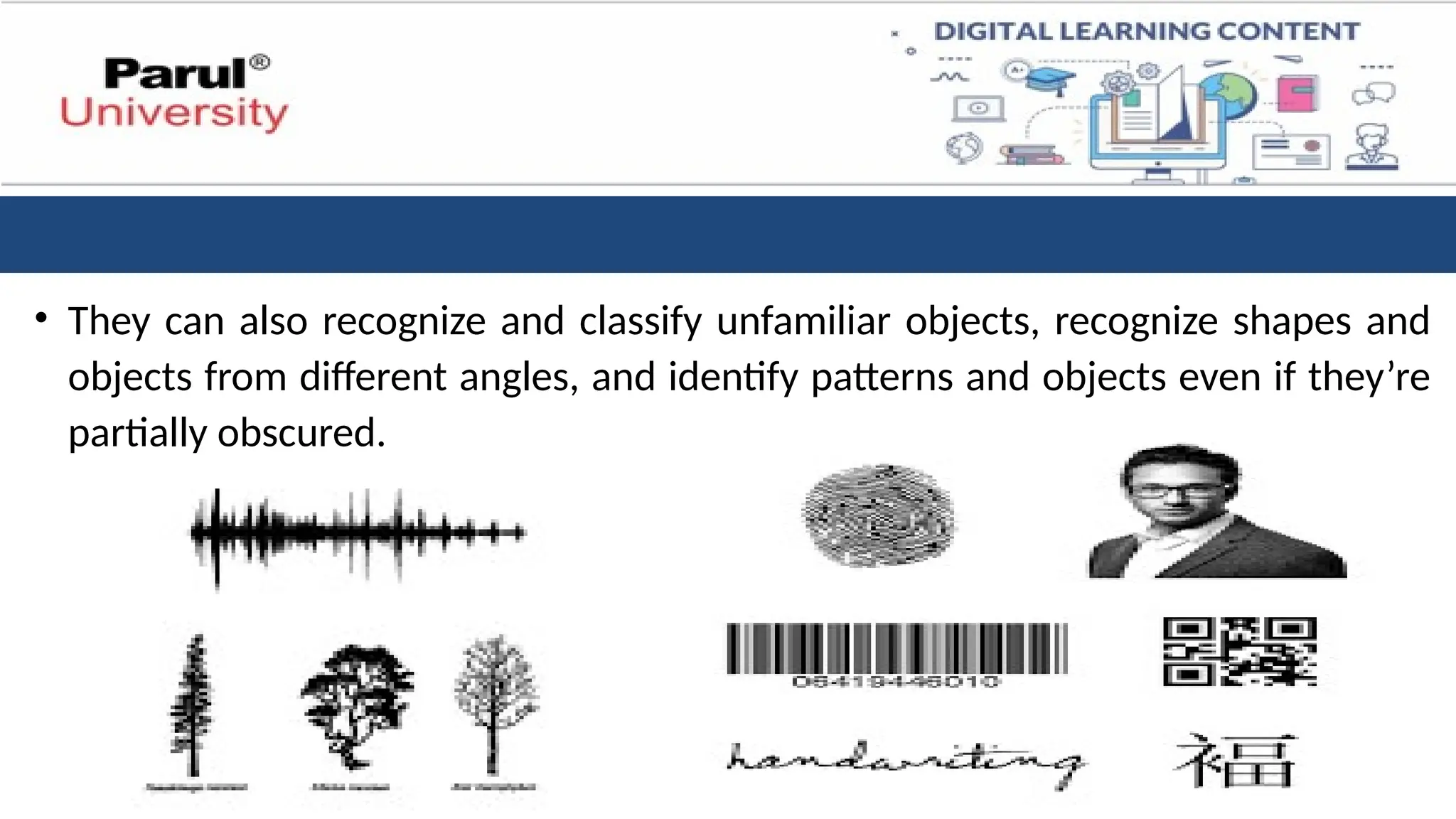
• They canalso recognize and classify unfamiliar objects, recognize shapes and
objects from different angles, and identify patterns and objects even if they’re
partially obscured.
6.
Examples of PRTasks
1. Character Recognition
• Pattern – Image.
• Class – identity of character
2. Speech Recognition
• Pattern – 1-D signal (or its sampled version)
• Class – identity of speech units
• Pattern can become a sequence of feature vectors.
7.
3 Fingerprint basedidentity verification
• Pattern – image plus a identity claim
• Class – Yes / No
4 Video-based Surveillance
• Pattern – video sequence
• Class – e.g., level of alertness
8.
5 Credit Screening
•Pattern – Details of an applicant (for, e.g., credit card)
• Class – Yes / No
• Features: income, job history, level of credit, credit history etc.
6 Imposter detection (of, e.g., credit card)
• Pattern – A sequence of transactions
• Class – Yes / No
• Features: Amount of money, locations oftransactions, times between
transactions etc.
9.
7 Document Classification
•Pattern – A document and a query
• Class – Relevant or not (in general, rank)
• Features – word occurrence counts, word context etc.
• Spam filtering,
• diagnostics of machinery etc..
10.
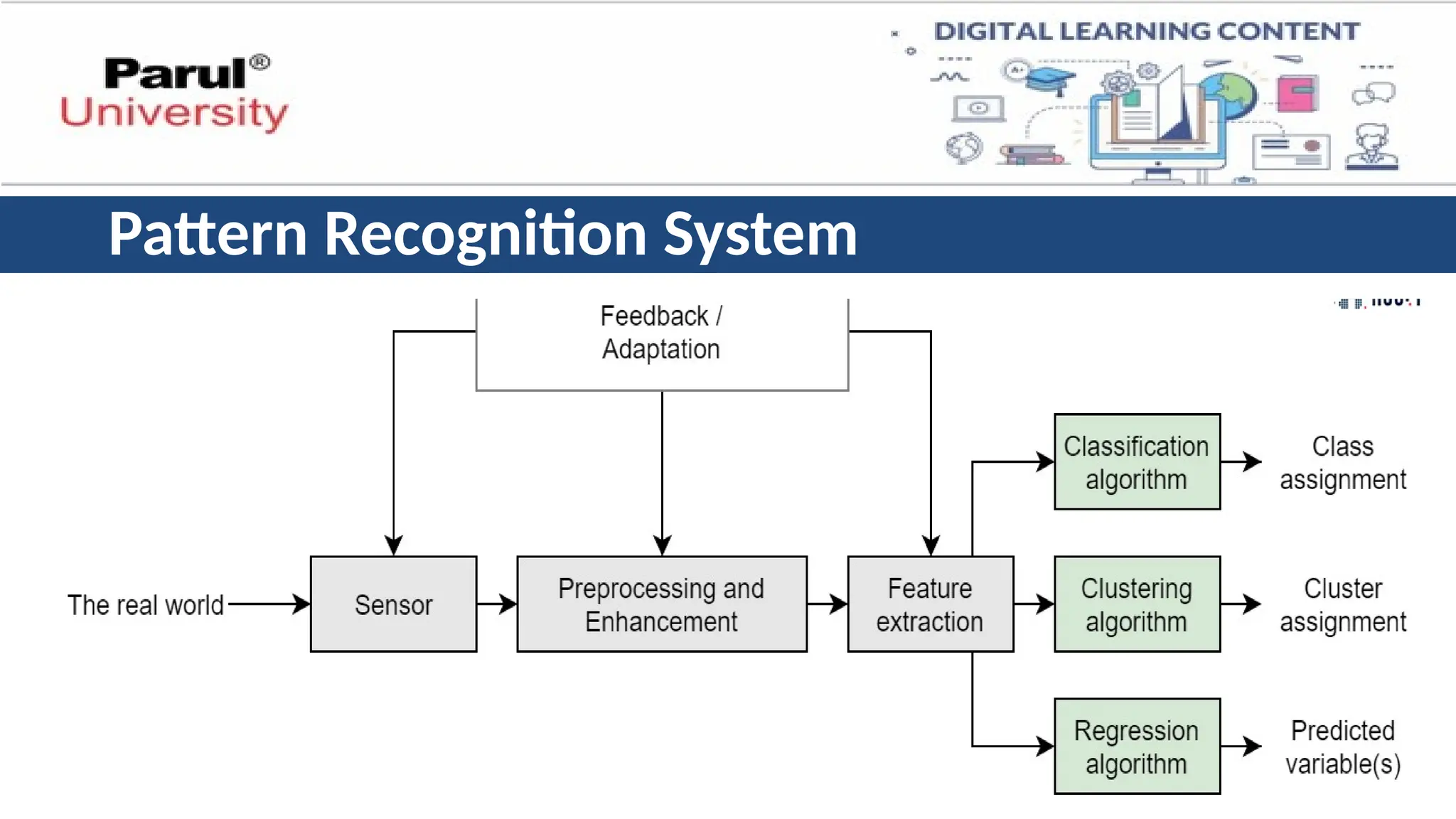
Pattern Recognition System
•The problem of pattern recognition is
🡪given some signal or information related to that pattern,
🡪then we need a machine to recognize a particular signal or information,
🡪extract it,
🡪classify it and
🡪to acquire and apply knowledge
Pattern 🡪 PR System 🡪 Class label
11.
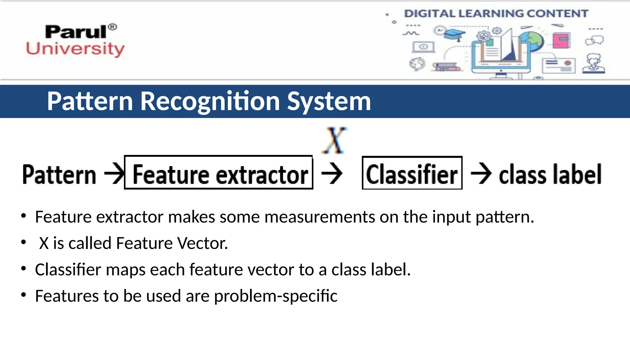
• Feature extractormakes some measurements on the input pattern.
• X is called Feature Vector.
• Classifier maps each feature vector to a class label.
• Features to be used are problem-specific
Pattern Recognition System
12.
• Features dependon the problem. Measure ‘relevant’ quantities.
• Some techniques available to extract ‘more relevant’ quantities from the
initial measurements. (e.g., PCA)
• After feature extraction each pattern is a vector
• Classifier is a function to map such vectors into class labels.
• Many general techniques of classifier design areavailable.
• Need to test and validate the final system.
Machine Perception
1. SensoryInput 🡪 Gathering data from various sensors like cameras,
microphones, or touch sensors.
2. Feature Extraction 🡪Analyzing the sensory data to identify relevant
patterns and characteristics.
3. Interpretation 🡪 Associating the extracted features with known concepts
or categories.
4. Decision Making 🡪 Using the interpreted information to make informed
decisions or take appropriate actions.
15.
Classification of PatternRecognition Systems
1. Supervised Learning
• The system is trained on labeled data to learn the mapping between
inputs and outputs.
2. Unsupervised Learning
• The system discovers patterns and structures in unlabeled data on its
own.
16.
3. Semi-Supervised Learning
•The system uses a combination of labeled and unlabeled data to
learn the patterns.
4. Reinforcement Learning
• The system learns by interacting with an environment and
receiving feedback on its actions.
17.
• This isthe most common approach for classification tasks.
• The system learns from labeled data, where each data point has a pre-defined category
(class label).
• Example: Image recognition using a supervised learning algorithm like a Convolutional
Neural Network (CNN).Training Data: A large collection of images labeled with their
content (e.g., cat, dog, car).
• Learning Process: The CNN analyzes the features (colors, shapes, textures) in the labeled
images and learns the patterns that differentiate between classes.
• Classification: When presented with a new, unseen image, the trained CNN uses its
learned knowledge to classify it into the most likely category (e.g., identifying a new
image as containing a dog).
1. Supervised Learning
18.
• Unlike supervisedlearning, the system doesn't have pre-defined class labels for the
data.
• It aims to find underlying patterns and group similar data points together without
prior knowledge of the categories.
• Example: Customer segmentation using a clustering algorithm like K-means.
• Data: Customer information like purchase history and demographics (age,
location).
• Learning Process: K-means analyzes the customer data and groups them into
clusters based on similarities in their purchase behavior and demographics.
• Applications: Identifying customer segments with similar characteristics for
targeted marketing campaigns.
2. Un-Supervised Learning
19.
• Semi-Supervised Classification:
•This approach combines labeled and unlabeled data for classification.
• It leverages the power of labeled data for guidance while utilizing the abundance
of unlabeled data to improve performance.
• Example: Sentiment analysis on social media posts.
• Data: A limited set of labeled posts (positive, negative, neutral) and a large
collection of unlabeled posts.
• Learning Process: The system first trains on the labeled data to learn basic
sentiment patterns. Then, it utilizes the unlabeled data to refine its
understanding of sentiment and improve classification accuracy.
3. Semi Supervised Learning
20.
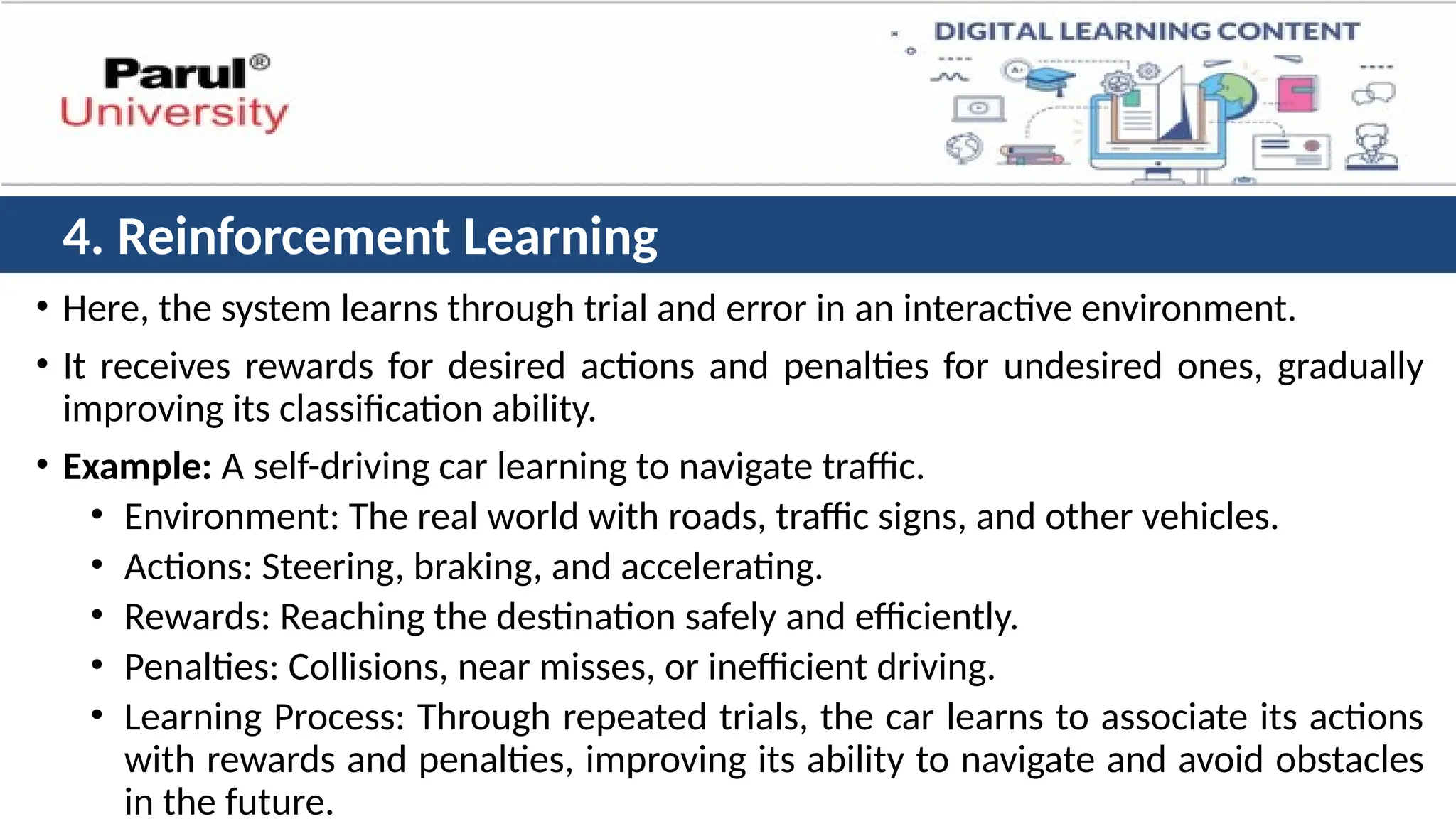
• Here, thesystem learns through trial and error in an interactive environment.
• It receives rewards for desired actions and penalties for undesired ones, gradually
improving its classification ability.
• Example: A self-driving car learning to navigate traffic.
• Environment: The real world with roads, traffic signs, and other vehicles.
• Actions: Steering, braking, and accelerating.
• Rewards: Reaching the destination safely and efficiently.
• Penalties: Collisions, near misses, or inefficient driving.
• Learning Process: Through repeated trials, the car learns to associate its actions
with rewards and penalties, improving its ability to navigate and avoid obstacles
in the future.
4. Reinforcement Learning
21.
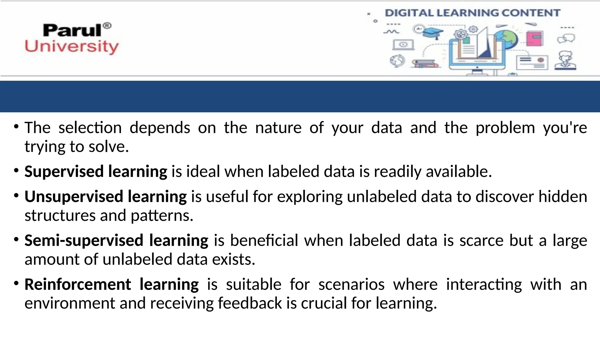
• The selectiondepends on the nature of your data and the problem you're
trying to solve.
• Supervised learning is ideal when labeled data is readily available.
• Unsupervised learning is useful for exploring unlabeled data to discover hidden
structures and patterns.
• Semi-supervised learning is beneficial when labeled data is scarce but a large
amount of unlabeled data exists.
• Reinforcement learning is suitable for scenarios where interacting with an
environment and receiving feedback is crucial for learning.
Step-1: Preprocessing:
• ProblemStatement: Clearly identify the task your system needs to perform.
For example, classifying handwritten digits (0-9) based on their image pixels.
• Data Characteristics: Understand the type of data you'll be working with
(images, text, sensor readings). Analyze its size, complexity, and potential
challenges (noise, missing values).
• Data Cleaning: Address inconsistencies and errors in your data. This might
involve handling missing values, outliers, and normalization (scaling data to a
specific range).
24.
Step-2: Feature Extraction:
•Identify and extract relevant features from the data that will be used for
classification. In our example, features might be pixel intensities at specific
locations in the image.
• Choose an appropriate classification algorithm based on the nature of your
problem and data. Popular options include:
• K-Nearest Neighbors (KNN): Classifies data points based on the majority class
of their nearest neighbors in the feature space.
25.
• Support VectorMachines (SVM): Finds the optimal hyperplane that separates
different classes with the maximum margin.
• Decision Trees: Learns a tree-like structure where decisions are made based on
feature values to classify data points.
• Deep Learning Models (CNNs): Utilize artificial neural networks specifically
designed for image recognition tasks.
26.
Step-3: Model Training:
•Train your chosen model on a labeled dataset.
• This dataset contains examples with pre-defined class labels (e.g., images of
handwritten digits labeled as 0, 1, 2, etc.).
• The model learns the relationships between features and class labels.
• Splitting Data: Divide your labeled data into training and testing sets.
• The training set is used to train the model, while the testing set is used to
evaluate its performance on unseen data.
27.
Step- 4. ModelEvaluation:
• Evaluate the performance of your trained model on the testing set. Common
metrics include:
• Accuracy: The percentage of correctly classified data points.
• Precision: The proportion of true positives among predicted positives (avoiding false
positives).
• Recall: The proportion of true positives identified out of all actual positives (avoiding
false negatives).
• Based on the evaluation, you might need to adjust the model parameters or try
a different classification algorithm if performance is unsatisfactory.
28.
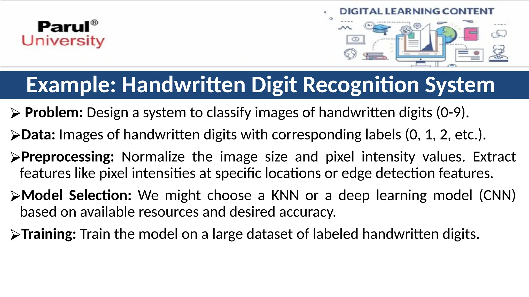
Example: Handwritten DigitRecognition System
⮚ Problem: Design a system to classify images of handwritten digits (0-9).
⮚Data: Images of handwritten digits with corresponding labels (0, 1, 2, etc.).
⮚Preprocessing: Normalize the image size and pixel intensity values. Extract
features like pixel intensities at specific locations or edge detection features.
⮚Model Selection: We might choose a KNN or a deep learning model (CNN)
based on available resources and desired accuracy.
⮚Training: Train the model on a large dataset of labeled handwritten digits.
29.
⮚Evaluation: Evaluate themodel's accuracy on a separate testing set. We might
need to adjust hyperparameters or try a different model if accuracy is low.
⮚Deployment: Deploy the model to classify new, unseen handwritten digits.
⮚Monitoring: Monitor the system's performance over time and retrain the
model if necessary.
30.
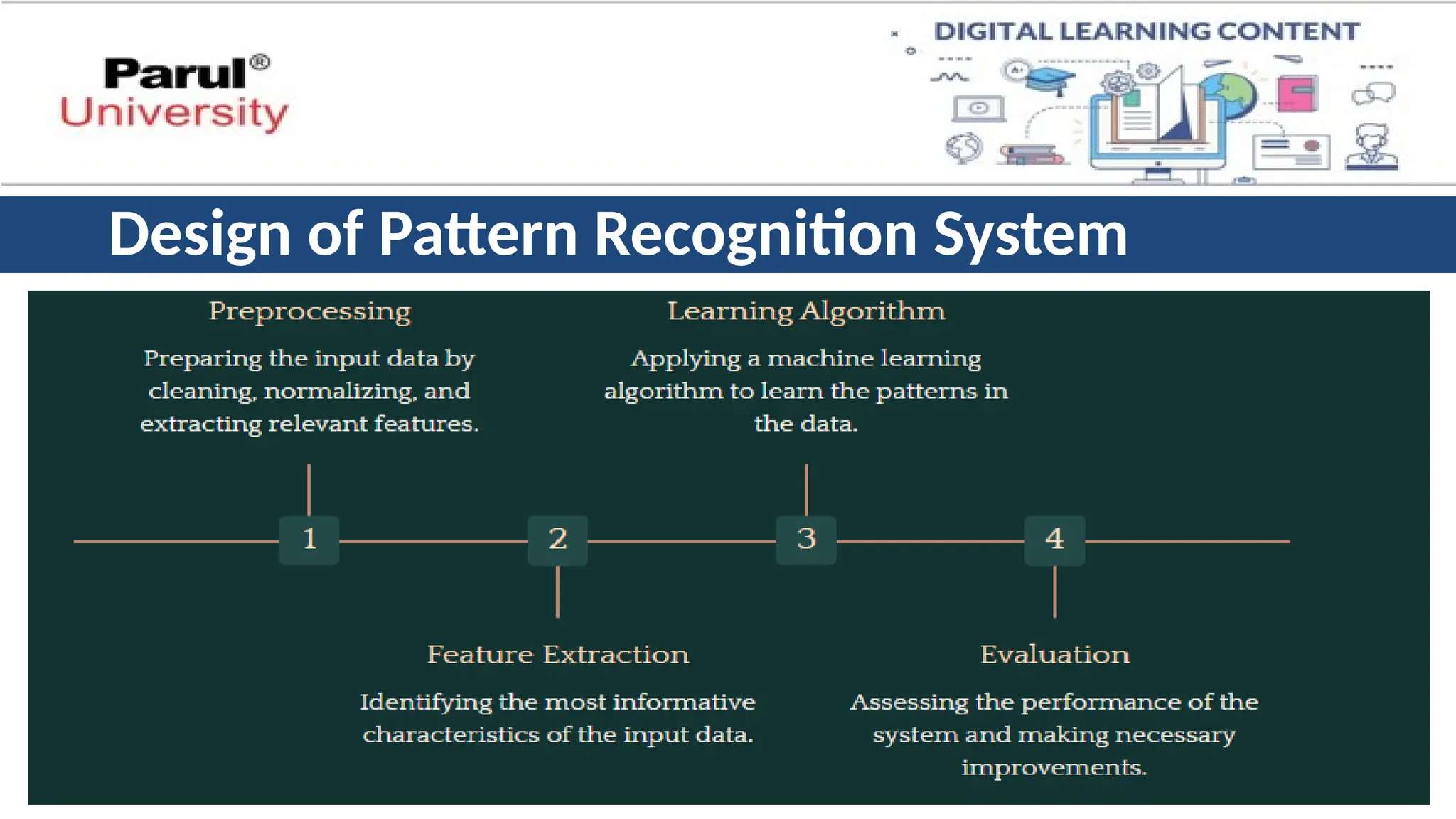
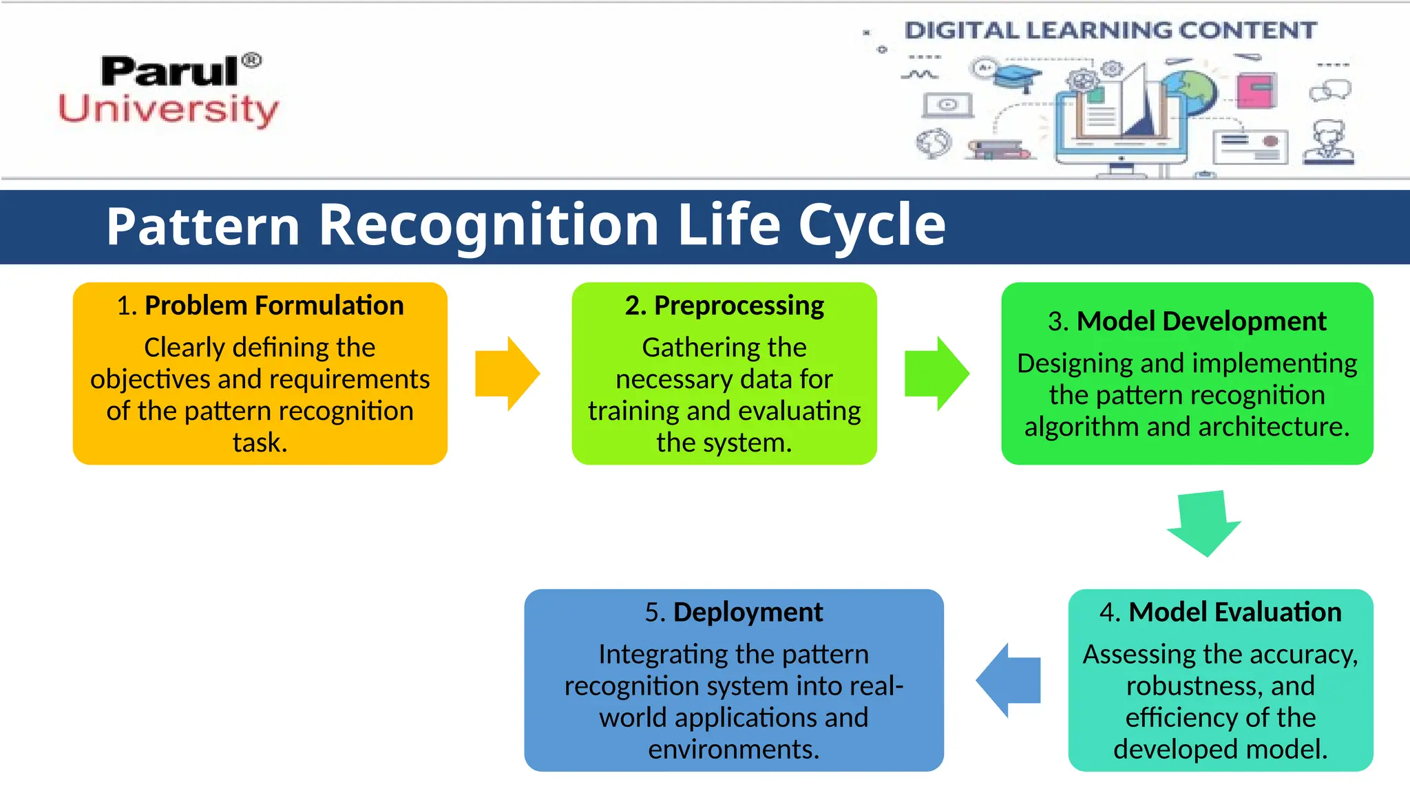
Pattern Recognition LifeCycle
1. Problem Formulation
Clearly defining the
objectives and requirements
of the pattern recognition
task.
2. Preprocessing
Gathering the
necessary data for
training and evaluating
the system.
3. Model Development
Designing and implementing
the pattern recognition
algorithm and architecture.
4. Model Evaluation
Assessing the accuracy,
robustness, and
efficiency of the
developed model.
5. Deployment
Integrating the pattern
recognition system into real-
world applications and
environments.
31.
• Pattern recognitionsystems evolve through a series of stages, transforming
raw data into meaningful classifications.
• Let's delve into the life cycle with an illustrative example:
Stage-1. Problem Definition and Data Acquisition (Example: Spam Filter):
• Problem: Build a system to automatically classify emails as spam or not spam.
• Data Acquisition: Collect a large corpus of labeled emails, including both
spam and legitimate emails. Here, each email is associated with a label (spam
or not spam).
32.
Stage-2. Preprocessing (Cleaningand Feature Extraction):
• Cleaning: Remove irrelevant information like email signatures or
advertisements.
• Address formatting inconsistencies and missing values.
• Feature Extraction: Identify and extract features that differentiate spam
from legitimate emails. These might include:
• Presence of certain keywords like "free" or "urgent"
• Sender address (known spammer list)
• Attachment types (executable files)
• Content analysis (suspicious links, unusual formatting)
33.
Stage - 3.Model Development and Training (Choosing the Right Weapon):
• Model Selection: Choose a classification algorithm suited for text
data. Options include:
• Naive Bayes: Effective for classifying text based on word probabilities.
• Support Vector Machines (SVM): Efficiently separates spam and legitimate
emails in a high-dimensional feature space.
• Training: Train the chosen model on the labeled email dataset. The model
learns the relationships between features (keywords, sender, etc.) and the
corresponding class label (spam or not spam).
34.
Stage - 4.Model Evaluation and Refinement (Testing and Tuning):
• Evaluation: Evaluate the model's performance on a separate testing
set of labeled emails. Calculate metrics like accuracy, precision, and
recall.
• Refinement: Analyze the evaluation results. If performance is
unsatisfactory, you might:
• Refine feature extraction techniques.
• Adjust model hyperparameters.
• Experiment with alternative classification algorithms.
35.
Stage - 5.Deployment and Monitoring (Putting it to Work and
Keeping an Eye Out):
• Deployment: Integrate the trained model into the spam filter system.
• Monitoring: Continuously monitor the system's performance over
time. This might involve analyzing false positives (legitimate emails
marked as spam) or false negatives (spam emails slipping through).
• Adaptation: As new spam tactics emerge, retrain the model with
updated data containing new keywords or sender addresses used by
spammers.
36.
• Improvement: Exploreadvanced techniques like ensemble learning
(combining multiple models) to further enhance the filter's accuracy.
• This life cycle is iterative. As new data becomes available and spam
tactics evolve, the system needs to be continuously refined and
improved to maintain its effectiveness.
37.
Statistical Pattern Recognition
•Statistical pattern recognition is a branch of pattern recognition that uses
statistical methods to analyze and classify patterns in data.
• Statistical pattern recognition is a powerful field that combines mathematics,
computer science, and real-world problem-solving.
• It relies heavily on probability theory and concepts like the Gaussian distribution
(normal distribution) to model the data and make classification decisions.
• This approach is particularly useful when the data exhibits inherent variability
and randomness.
• It provides the tools to analyze and make sense of complex data, enabling
insights and informed decision-making across various domains.
38.
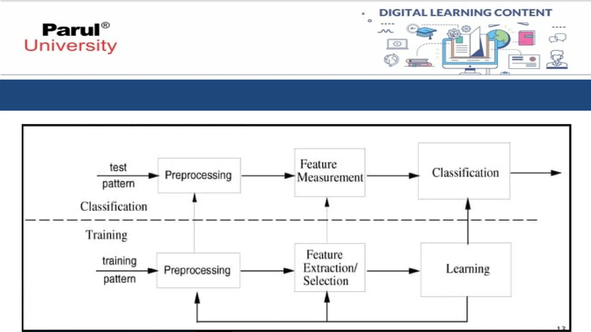
• In statisticalpattern recognition, a pattern is represented by a set of d
features, or attributes, viewed as a d-dimensional feature vector.
• Statistical decision theory are utilized to establish decision boundaries
between pattern classes.
• The recognition system is operated in two modes:
1. training (learning)
2. classification (testing)
40.
Probability Theory
• Akey concept in the field of pattern recognition is that of uncertainty.
• Probability theory is the foundation of statistical pattern recognition.
• It provides a framework for quantifying the likelihood of events occurring.
• It arises both through noise on measurements, as well as through the finite size
of data sets.
• Probability theory provides a consistent framework for the quantification and
manipulation of uncertainty and forms one of the central foundations for
pattern recognition
41.
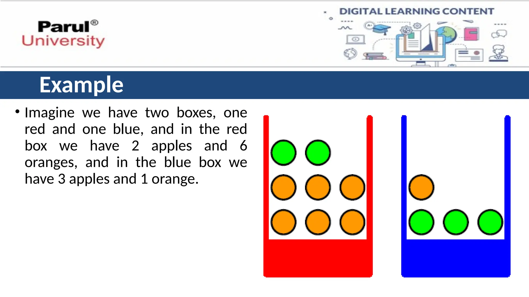
Example
• Imagine wehave two boxes, one
red and one blue, and in the red
box we have 2 apples and 6
oranges, and in the blue box we
have 3 apples and 1 orange.
42.
• Now supposewe randomly pick one of the boxes and from that box we
randomly select an item of fruit, and having observed which sort of fruit it is
we replace it in the box from which it came.
• We could imagine repeating this process many times.
• Let us suppose that in so doing we pick the red box 40% of the time and we
pick the blue box 60% of the time, and that when we remove an item of fruit
from a box we are equally likely to select any of the pieces of fruit in the box.
43.
• In thisexample, the identity of the box that will be chosen is a random
variable, which we shall denote by B.
• This random variable can take one of two possible values, namely r
(corresponding to the red box) or b (corresponding to the blue box).
• Similarly, the identity of the fruit is also a random variable and will be
denoted by F. It can take either of the values a (for apple) or o (for orange).
44.
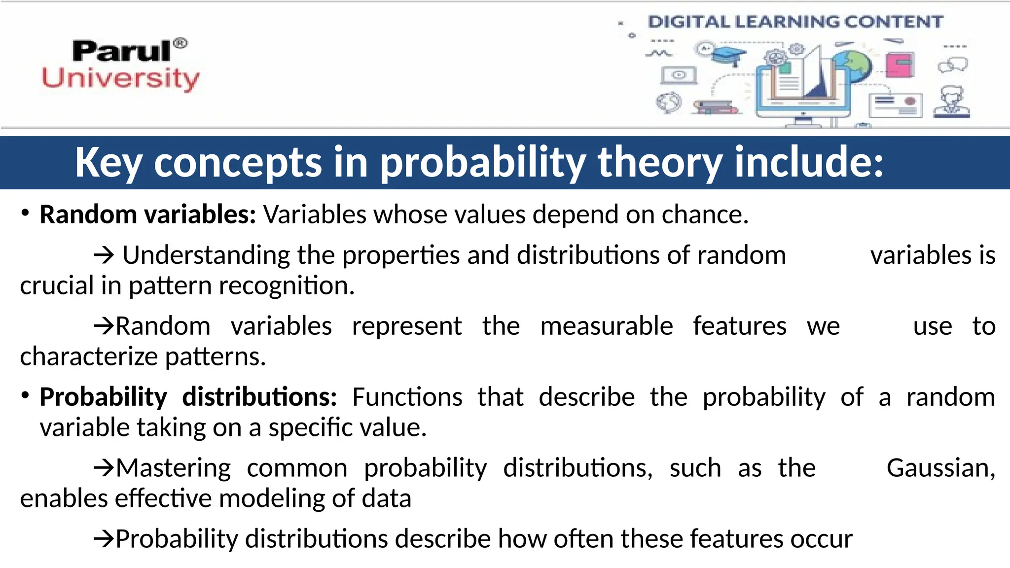
Key concepts inprobability theory include:
• Random variables: Variables whose values depend on chance.
🡪 Understanding the properties and distributions of random variables is
crucial in pattern recognition.
🡪Random variables represent the measurable features we use to
characterize patterns.
• Probability distributions: Functions that describe the probability of a random
variable taking on a specific value.
🡪Mastering common probability distributions, such as the Gaussian,
enables effective modeling of data
🡪Probability distributions describe how often these features occur
45.
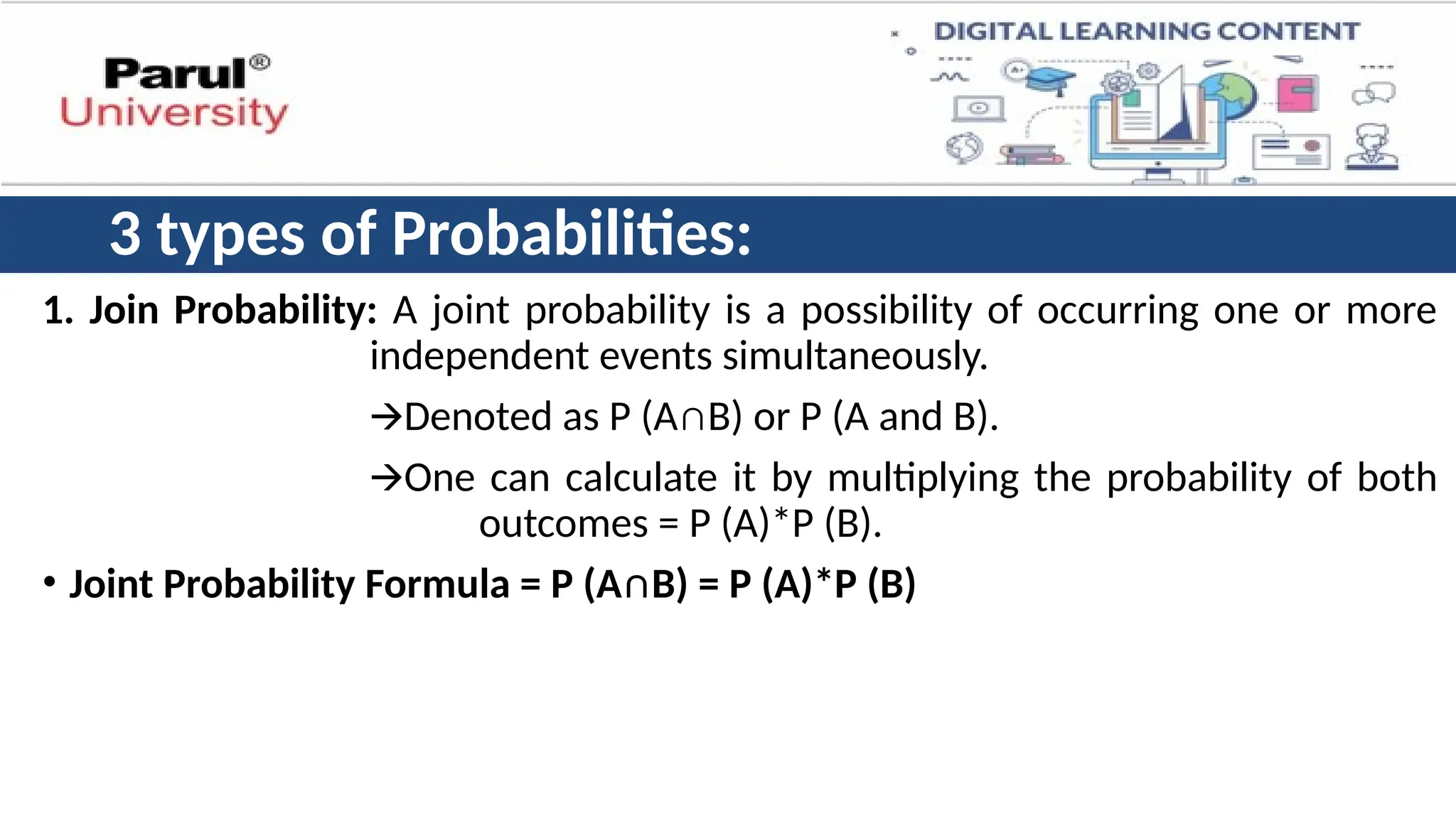
3 types ofProbabilities:
1. Join Probability: A joint probability is a possibility of occurring one or more
independent events simultaneously.
🡪Denoted as P (A∩B) or P (A and B).
🡪One can calculate it by multiplying the probability of both
outcomes = P (A)*P (B).
• Joint Probability Formula = P (A∩B) = P (A)*P (B)
46.
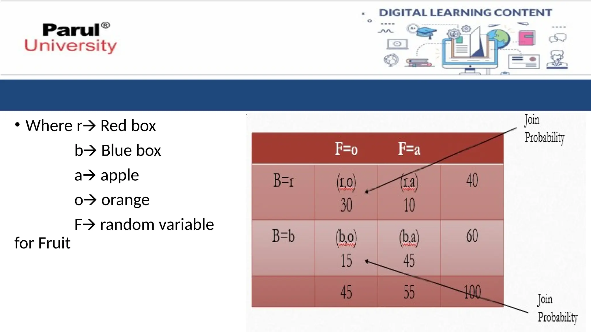
• Where rRed box
🡪
b Blue box
🡪
a apple
🡪
o orange
🡪
F random variable
🡪
for Fruit
47.
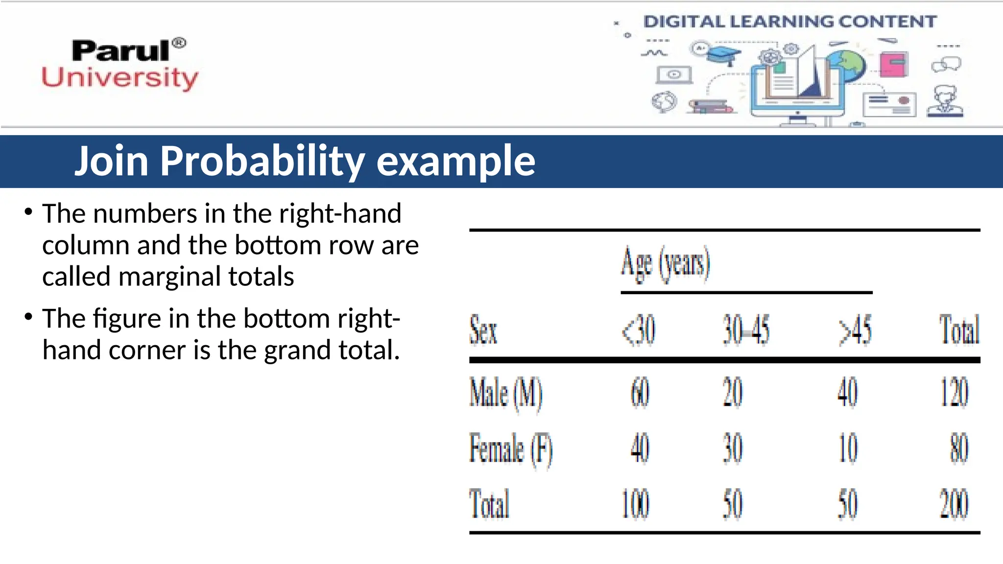
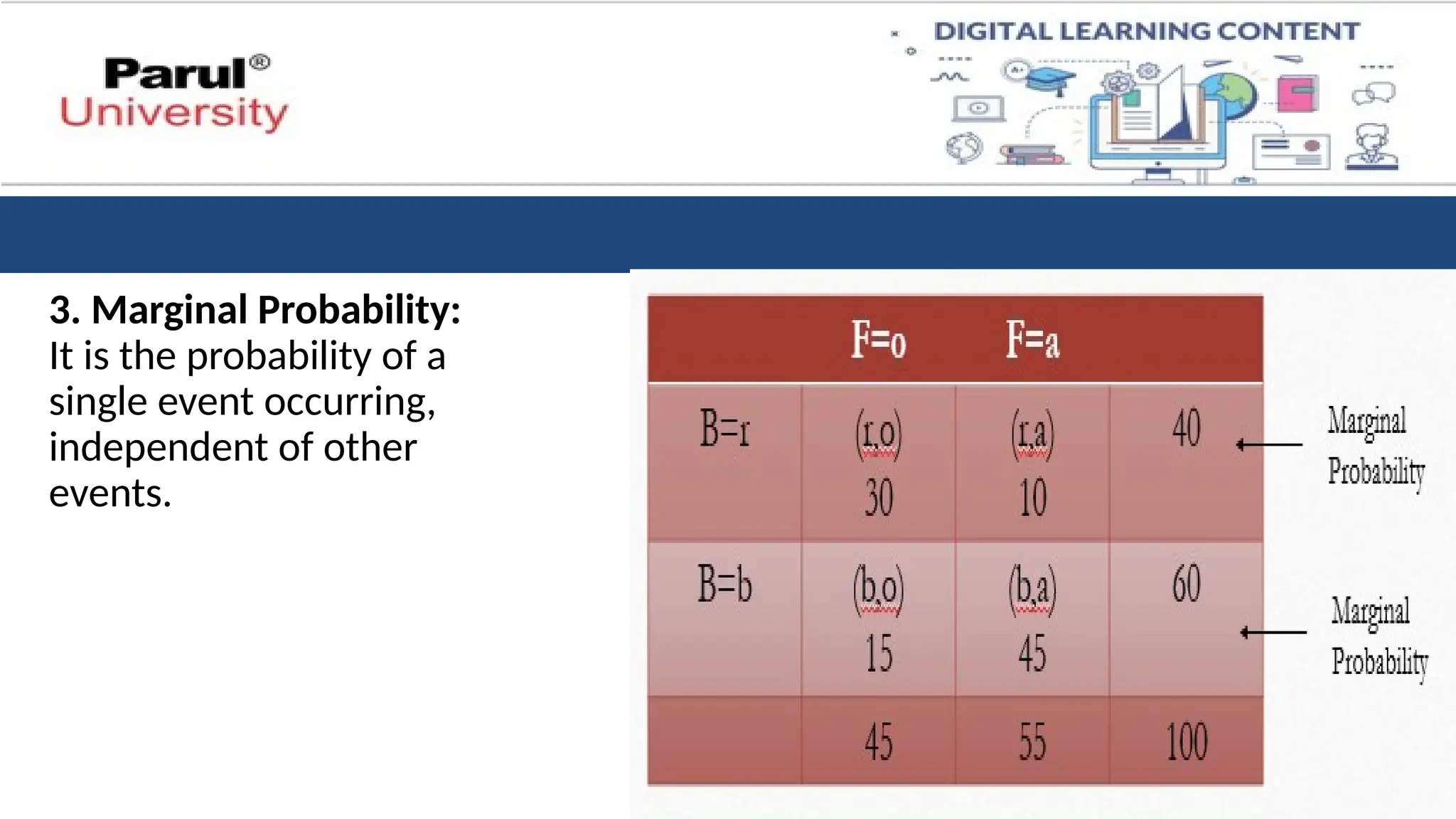
Join Probability example
•The numbers in the right-hand
column and the bottom row are
called marginal totals
• The figure in the bottom right-
hand corner is the grand total.
48.
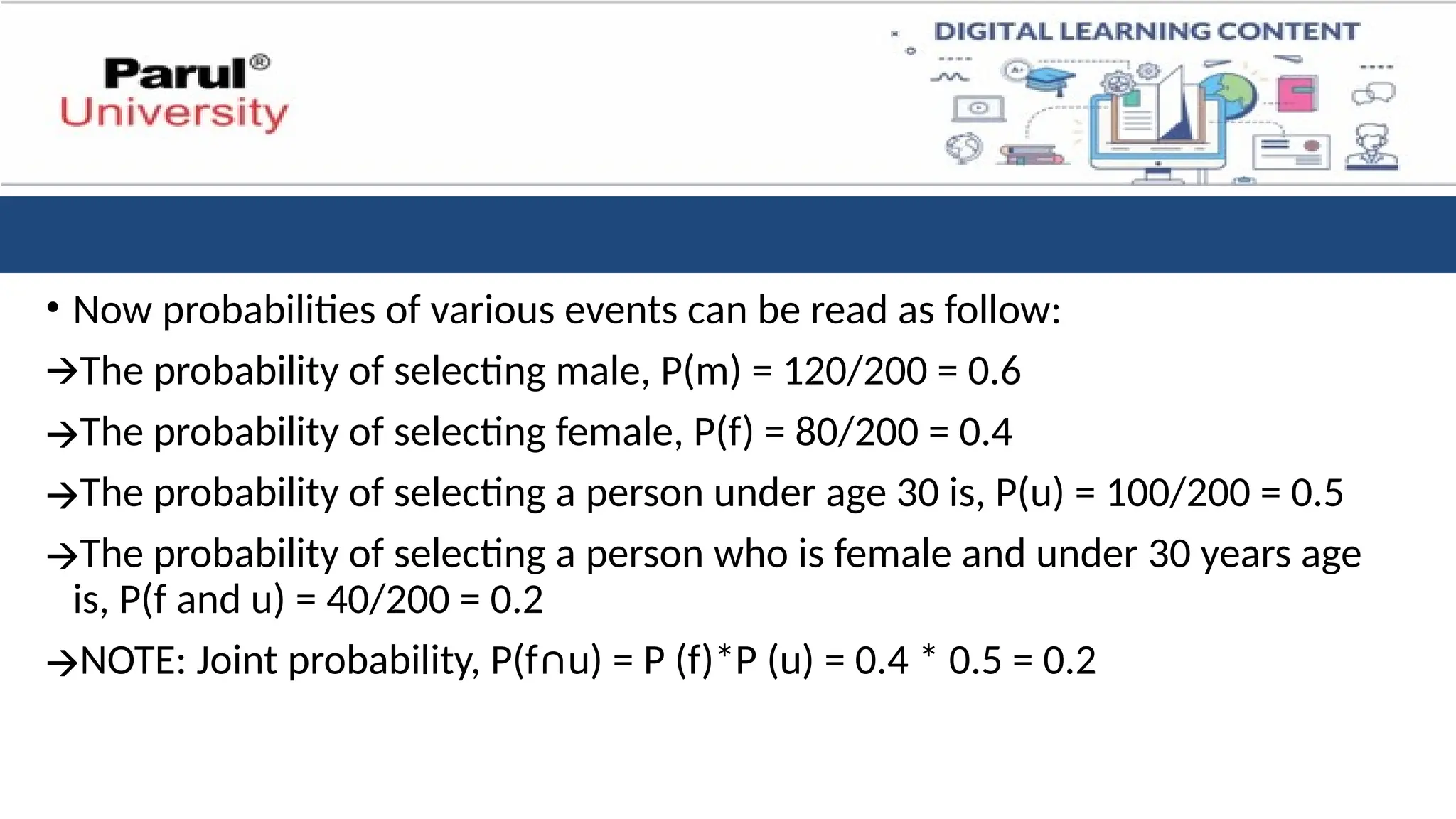
• Now probabilitiesof various events can be read as follow:
🡪The probability of selecting male, P(m) = 120/200 = 0.6
🡪The probability of selecting female, P(f) = 80/200 = 0.4
🡪The probability of selecting a person under age 30 is, P(u) = 100/200 = 0.5
🡪The probability of selecting a person who is female and under 30 years age
is, P(f and u) = 40/200 = 0.2
🡪NOTE: Joint probability, P(f∩u) = P (f)*P (u) = 0.4 * 0.5 = 0.2
49.
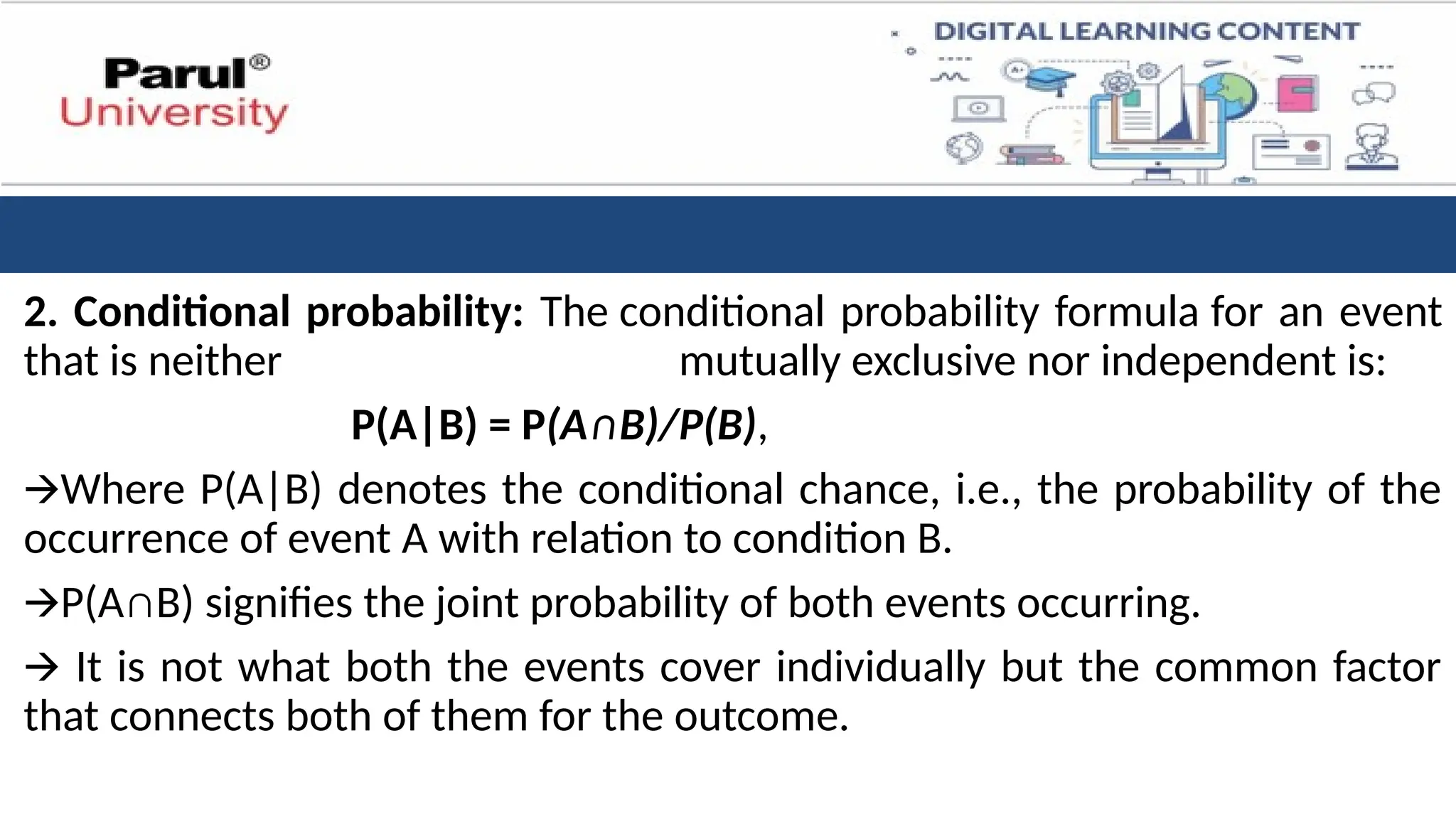
2. Conditional probability:The conditional probability formula for an event
that is neither mutually exclusive nor independent is:
P(A|B) = P(A∩B)/P(B),
🡪Where P(A|B) denotes the conditional chance, i.e., the probability of the
occurrence of event A with relation to condition B.
🡪P(A∩B) signifies the joint probability of both events occurring.
🡪 It is not what both the events cover individually but the common factor
that connects both of them for the outcome.
50.
🡪P(B) is theprobability of B.
🡪The probability of one event occurring given that another event has
already occurred.
🡪The ability to calculate the probability of an event given the occurrence
of another event is crucial.
🡪Conditional probability helps us understand how the occurrence of
one pattern influences the likelihood of another.
51.
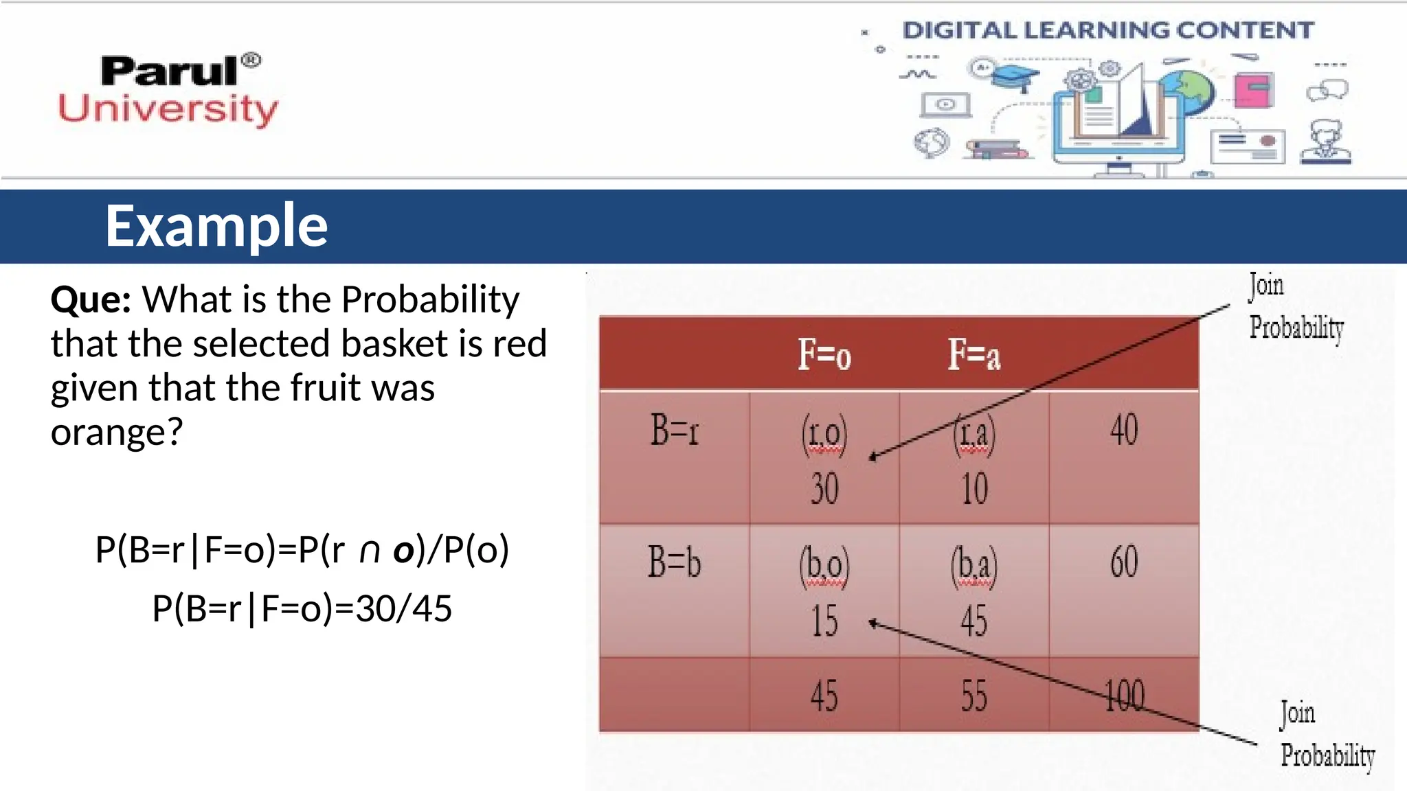
Example
Que: What isthe Probability
that the selected basket is red
given that the fruit was
orange?
P(B=r|F=o)=P(r ∩ o)/P(o)
P(B=r|F=o)=30/45
Gaussian Distribution
• TheGaussian distribution, also known as the normal distribution, is a
bell-shaped probability distribution.
• The Gaussian distribution is a fundamental concept in statistics and
pattern recognition.
• Many natural phenomena exhibit Gaussian-like behavior, making it a
suitable model for representing the variability observed in features used
for pattern classification.
• The mean indicates the average value of the feature, while the standard
deviation reflects the degree of spread around the mean.
54.
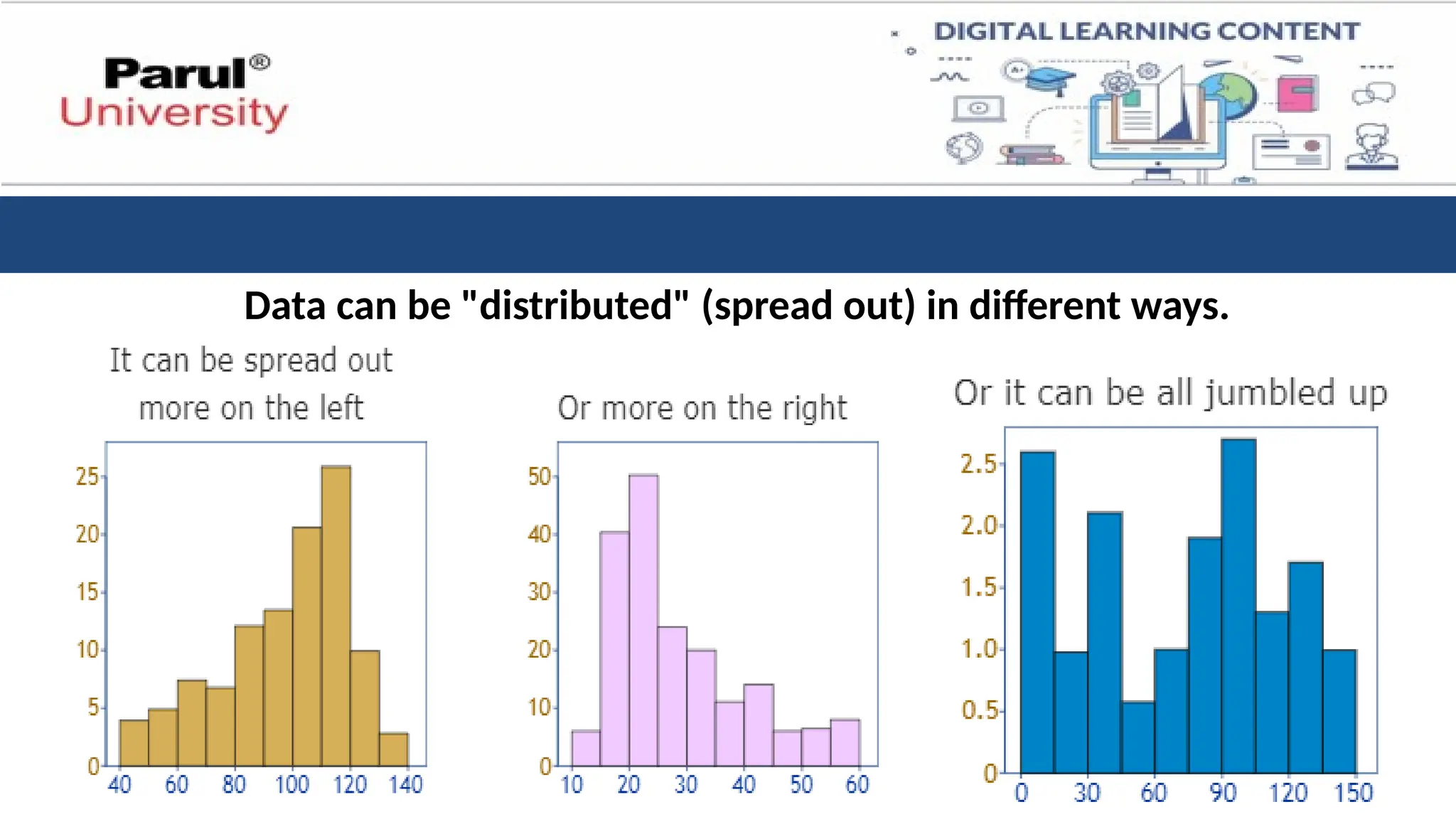
Data can be"distributed" (spread out) in different ways.
55.
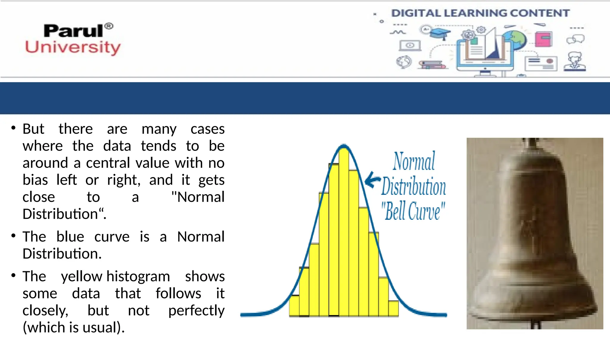
• But thereare many cases
where the data tends to be
around a central value with no
bias left or right, and it gets
close to a "Normal
Distribution“.
• The blue curve is a Normal
Distribution.
• The yellow histogram shows
some data that follows it
closely, but not perfectly
(which is usual).
56.
• It iswidely used in statistical pattern recognition due to its prevalence in
real-world data.
• Defining Characteristics: The Gaussian distribution is symmetrical around the
mean, with the peak corresponding to the most likely value and the tails tapering
off as the values move away from the center.
• Importance in Pattern Recognition: Many real-world data, such as
measurements, errors, and natural variations, can be modeled using the Gaussian
distribution, making it a fundamental tool in statistical pattern recognition.
57.
• Applications: TheGaussian distributions are widely used in areas such
as image processing, speech recognition, and bioinformatics.
• The Gaussian distribution is characterized by two parameters:
• Mean (μ): The center of the distribution.
• Standard deviation (σ): The spread of the distribution.
58.
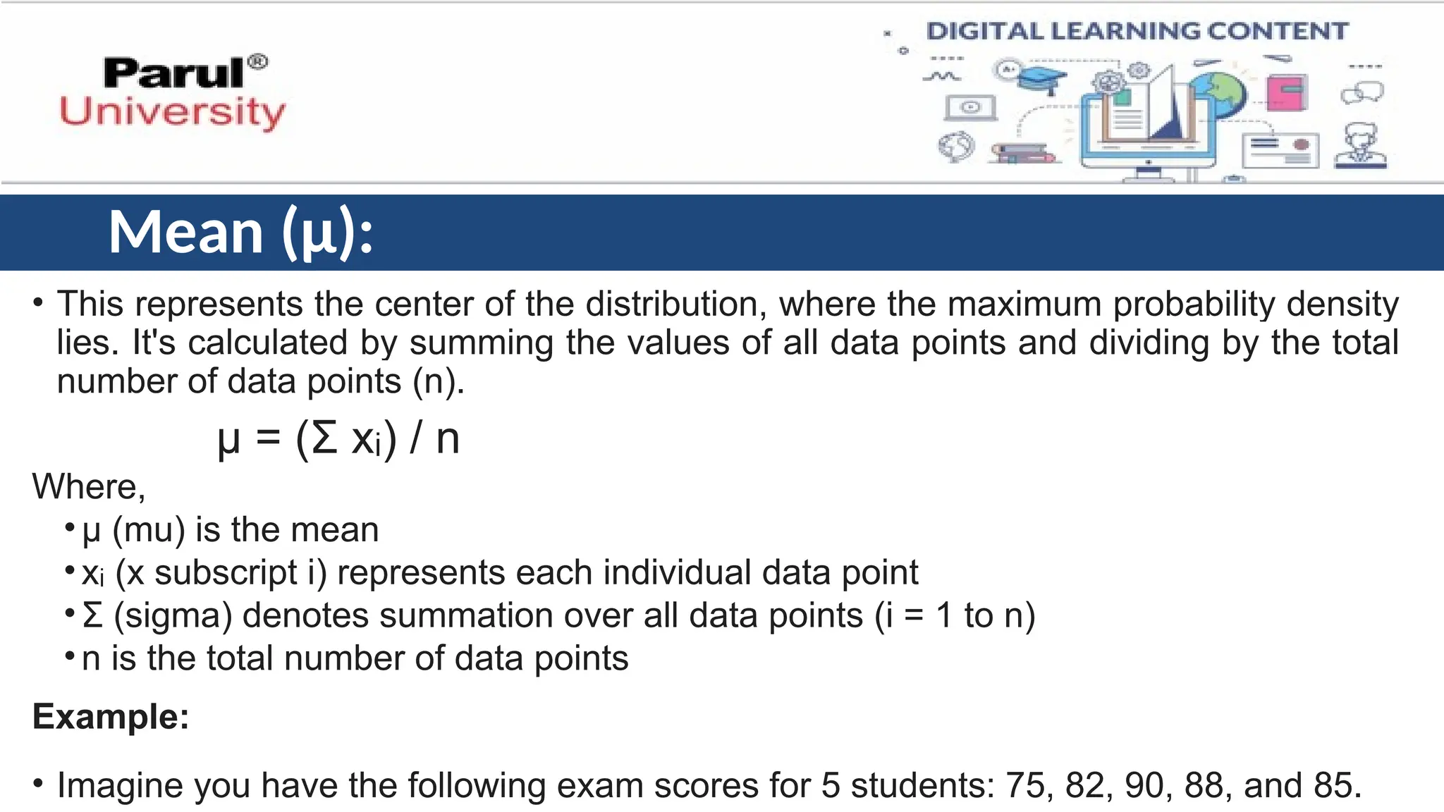
Mean (μ):
• Thisrepresents the center of the distribution, where the maximum probability density
lies. It's calculated by summing the values of all data points and dividing by the total
number of data points (n).
μ = (Σ x ) / n
ᵢ
Where,
•μ (mu) is the mean
•x (x subscript i) represents each individual data point
ᵢ
•Σ (sigma) denotes summation over all data points (i = 1 to n)
•n is the total number of data points
Example:
• Imagine you have the following exam scores for 5 students: 75, 82, 90, 88, and 85.
59.
• We saythe data is "normally
distributed":
• mean = median = mode
• symmetry about the center
• 50% of values less than the mean
and 50% greater than the mean
60.
Standard Deviation (σ):
•The Standard Deviation is a measure of how spread out numbers are.
• This signifies the spread of the data around the mean.
• There are two common ways to calculate standard deviation,
(i) depending on whether you want the population standard deviation (σ)
reflecting the entire population, or
(ii) the sample standard deviation (s) reflecting a specific sample:
1. Population Standard Deviation (σ):
σ = √[Σ (x - μ)² / n]
ᵢ
61.
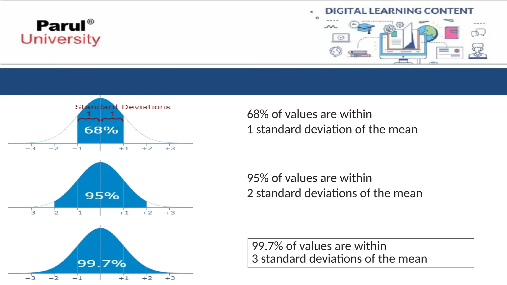
68% of valuesare within
1 standard deviation of the mean
95% of values are within
2 standard deviations of the mean
99.7% of values are within
3 standard deviations of the mean
62.
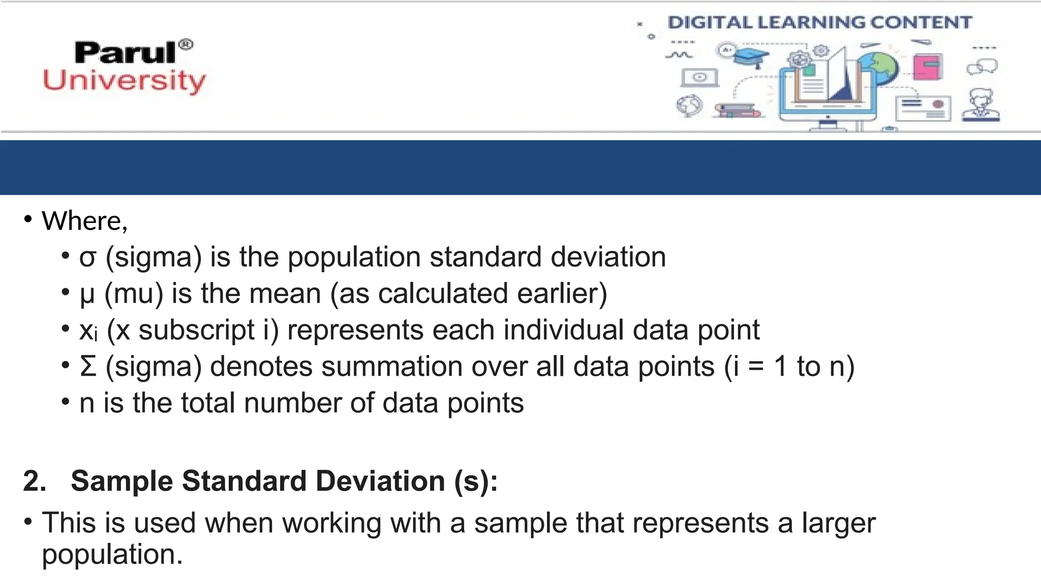
• Where,
• σ(sigma) is the population standard deviation
• μ (mu) is the mean (as calculated earlier)
• x (x subscript i) represents each individual data point
ᵢ
• Σ (sigma) denotes summation over all data points (i = 1 to n)
• n is the total number of data points
2. Sample Standard Deviation (s):
• This is used when working with a sample that represents a larger
population.
63.
s = √[Σ(xᵢ - μ)² / (n - 1)]
• where:
• s is the sample standard deviation
• μ (mu) is the mean (as calculated earlier)
• xᵢ (x subscript i) represents each individual data point
• Σ (sigma) denotes summation over all data points (i = 1 to n)
• n is the total number of data points
64.
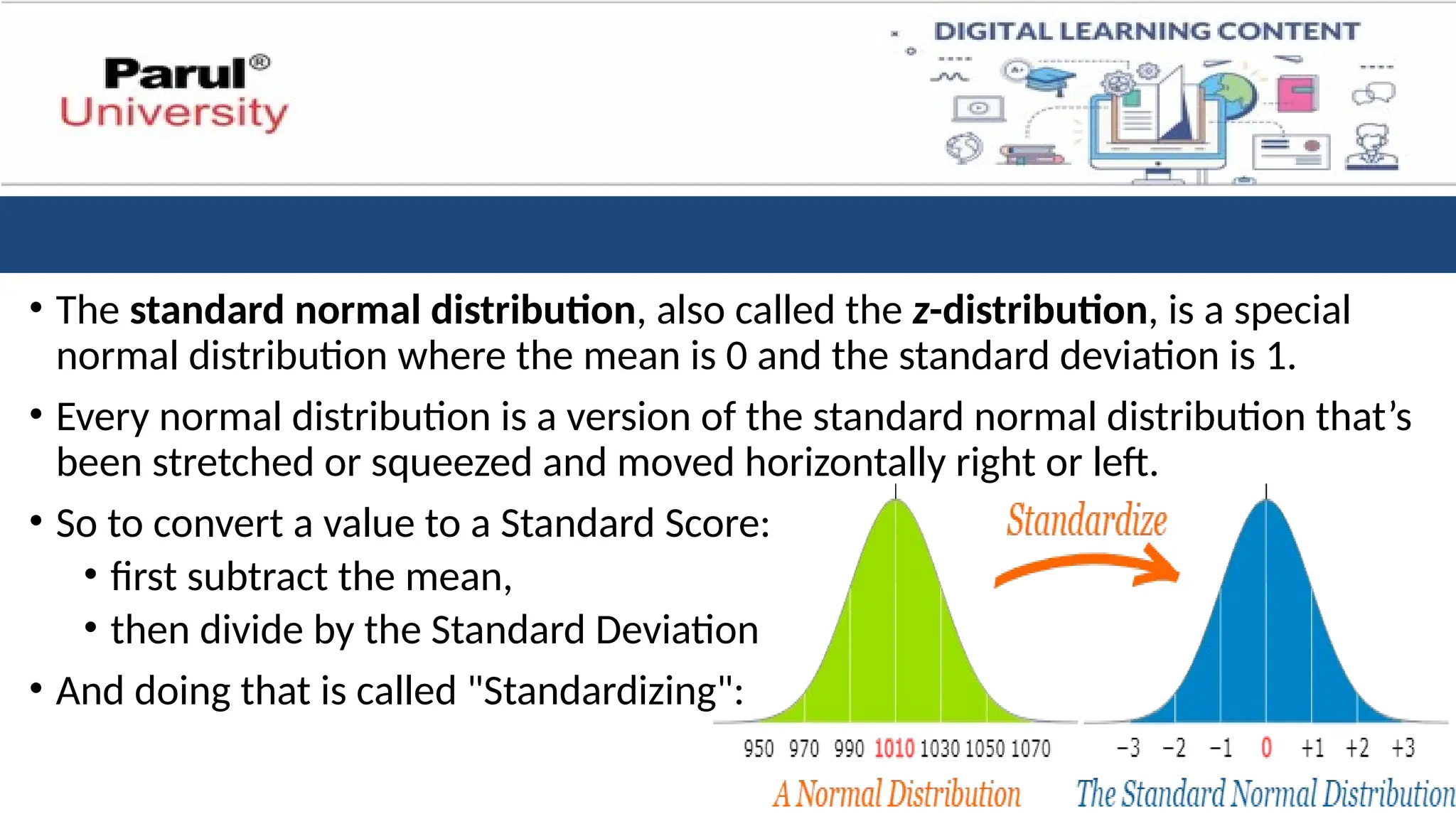
• The standardnormal distribution, also called the z-distribution, is a special
normal distribution where the mean is 0 and the standard deviation is 1.
• Every normal distribution is a version of the standard normal distribution that’s
been stretched or squeezed and moved horizontally right or left.
• So to convert a value to a Standard Score:
• first subtract the mean,
• then divide by the Standard Deviation
• And doing that is called "Standardizing":
65.
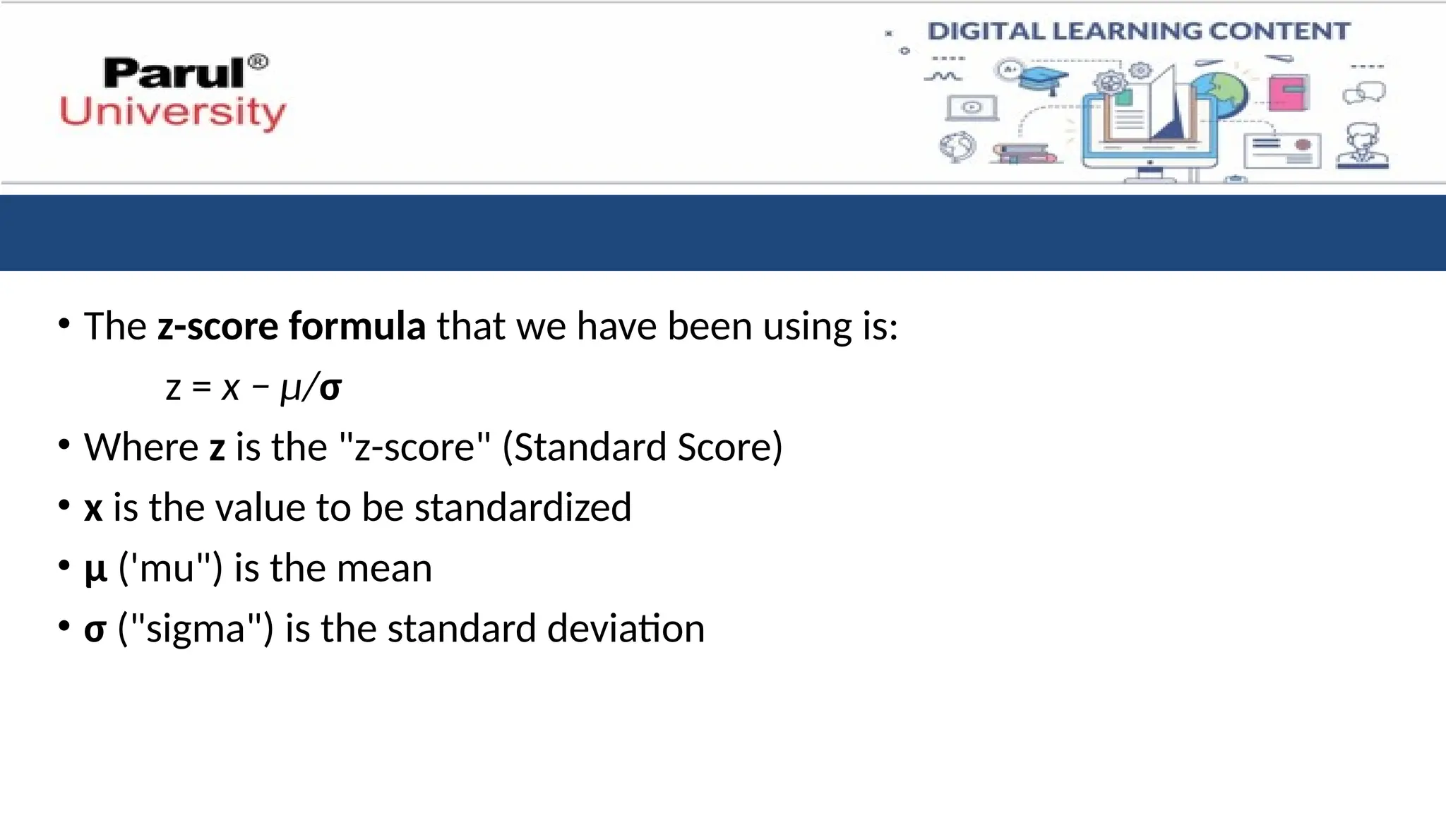
• The z-scoreformula that we have been using is:
z = x − μ/σ
• Where z is the "z-score" (Standard Score)
• x is the value to be standardized
• μ ('mu") is the mean
• σ ("sigma") is the standard deviation
66.
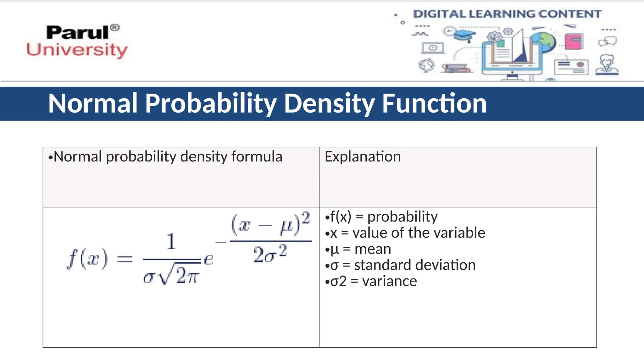
Normal Probability DensityFunction
•Normal probability density formula Explanation
•f(x) = probability
•x = value of the variable
•μ = mean
•σ = standard deviation
•σ2 = variance
67.
Bayes Decision Theoryand Classifiers
• Bayes' Decision Theory is a powerful statistical framework that enables
optimal decision-making by incorporating prior knowledge and new
evidence.
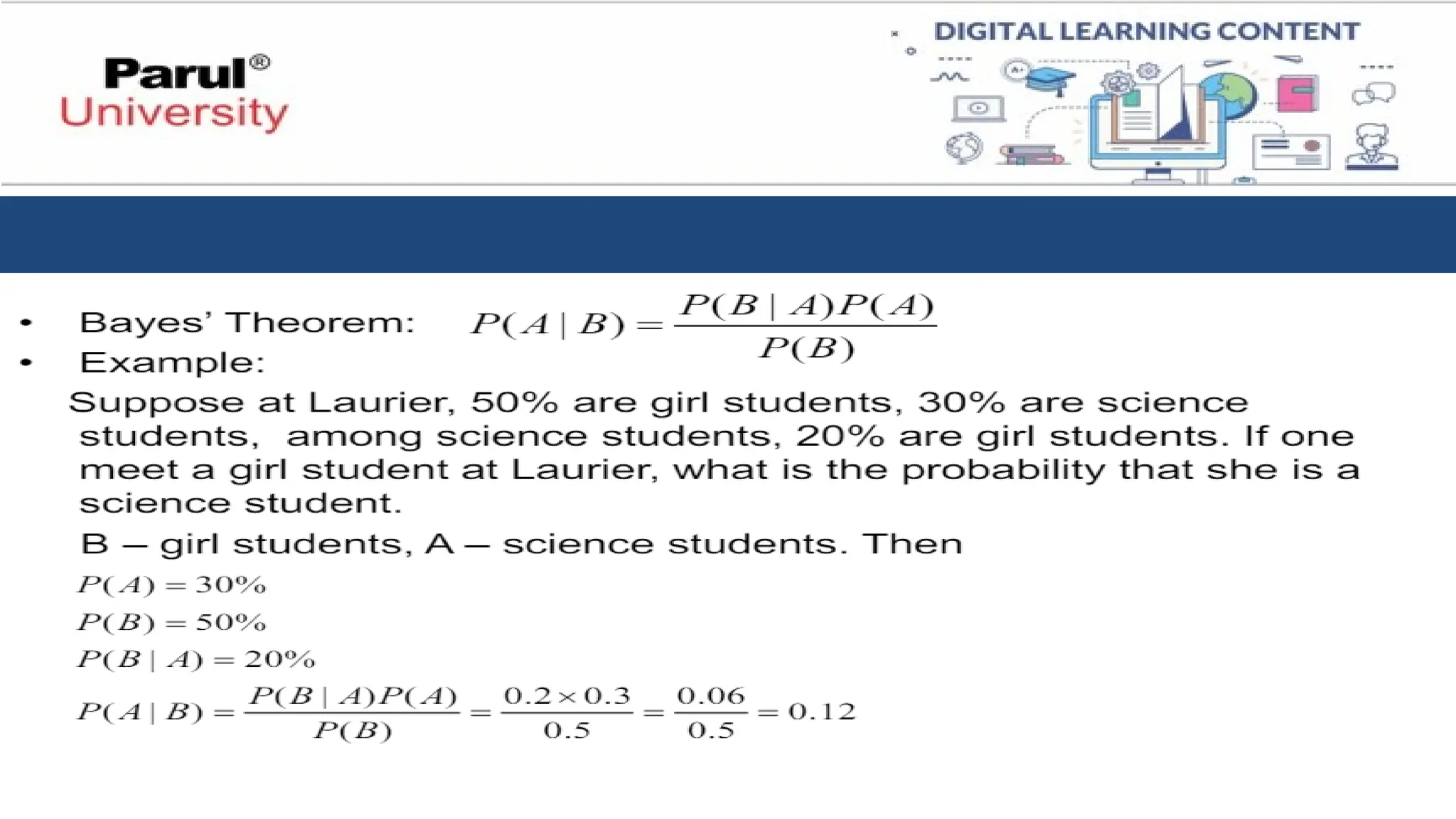
• It relies on the fundamental principle of Bayes' Theorem, which allows for
the calculation of posterior probabilities based on prior probabilities and
observed data.
• For example, in a medical diagnosis scenario, the prior probabilities could be
the known prevalence of a disease in the population. New evidence, such as
the results of a medical test, would then be used to update the probabilities
and determine the most likely diagnosis and optimal course of treatment.
68.
• The keysteps in Bayes' Decision Theory are:
1) defining prior probabilities,
🡪 which represent the initial beliefs about the likelihood of different
outcomes
2) incorporating new evidence
🡪 incorporating new evidence or data to update the prior probabilities
and calculate the posterior probabilities
3) making a decision that minimizes the overall expected cost or
maximizes the expected benefit.
69.
• Here wehave to consider two types of probabilities
1. Prior Probability
2. Likelihood Probability
70.
Prior Probability
• Theprobability is calculated according to the past occurrences of the
outcomes (i.e. events). This is called the prior probability ("prior" meaning
"before").
• In other words, the prior probability refers to the probability in the past.
• Assume that someone asks who will be the winner of a future match
between two teams. Let A and B refer to the first or second team winning,
respectively.
• In the last 10 cup matches, A occurred 4 times and B occurred the remaining
6 times. So, what is the probability that A occurs in the next match?
71.
• Based onthe experience (i.e., the events that occurred in the past), the prior
probability that the first team (A) wins in the next match is:
P(A)=4/10
=0.4
• But the past events may not always hold, because the situation or context may
change.
• For example, team A could have won only 4 matches because there were some
injured players.
• When the next match comes, all of these injured players will have recovered.
Based on the current situation, the first team may win the next match with a
higher probability than the one calculated based on past events only.
72.
• The priorprobability measures the probability of the next action without
taking into consideration a current observation (i.e. the current situation).
• It's like predicting that a patient has a given disease based only on past doctors
visits.
• In other words, because the prior probability is solely calculated based on past
events (without present information), this can degrade the prediction value
quality.
• The past predictions of the two outcomes A and B may have occurred while
some conditions were satisfied, but at the current moment, these conditions
may not hold.
73.
Likelihood Probability
• Thelikelihood helps to answer the question:
🡪given some conditions, what is the probability that an outcome occurs? It
is denoted as follows:
P(X Ci)
∣
• Where X refers to the conditions, and Ci refers to the outcome.
• Because there may be multiple outcomes, the variable C is given the
subscript i.
• Under a set of conditions X, what is the probability that the outcome is Ci?
74.
• A drawbackof using only the likelihood is that it neglects experience (prior
probability), which is useful in many cases. So, a better way to do a prediction is
to combine them both.
P(Ci
)P(X∣Ci
)
• Bayesian Decision Theory (i.e. the Bayesian Decision Rule) predicts the outcome
not only based on previous observations, but also by taking into account the
current situation.
• The rule describes the most reasonable action to take based on an
observation.
75.
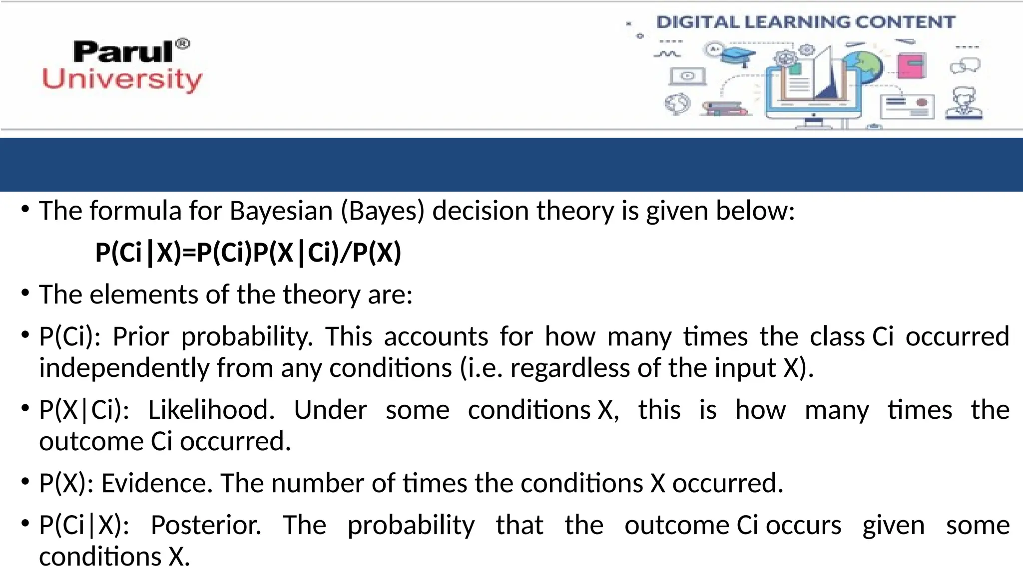
• The formulafor Bayesian (Bayes) decision theory is given below:
P(Ci X)=P(Ci)P(X Ci)/P(X)
∣ ∣
• The elements of the theory are:
• P(Ci): Prior probability. This accounts for how many times the class Ci occurred
independently from any conditions (i.e. regardless of the input X).
• P(X|Ci): Likelihood. Under some conditions X, this is how many times the
outcome Ci occurred.
• P(X): Evidence. The number of times the conditions X occurred.
• P(Ci|X): Posterior. The probability that the outcome Ci occurs given some
conditions X.
77.
• In classificationtasks, we strive for models that make the fewest
mistakes.
• However, there are two key ways to measure these mistakes:
• minimum error and
• minimum error rate.
• While they might sound similar, they have subtle differences, and the
optimal solution can vary depending on the chosen criterion.
78.
Gradient Descent Optimizer
•It is an iterative algorithm that is used to minimize a function by finding the
optimal parameters.
• Gradient Descent (GD) is a popular optimization algorithm used in machine
learning to minimize the loss function.
• It iteratively adjusts the model's parameters to find the optimal values that
minimize the difference between predicted and actual outputs.
• To implement a gradient descent algorithm, we require a cost function that needs
to be minimized, the number of iterations, a learning rate to determine the step
size at each iteration while moving towards the minimum, partial derivatives for
weight & bias to update the parameters at each iteration, and a prediction
function.
79.
Example
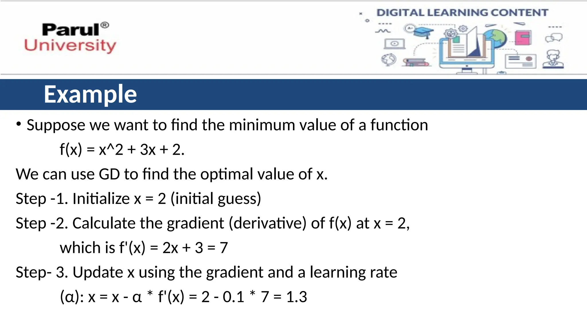
• Suppose wewant to find the minimum value of a function
f(x) = x^2 + 3x + 2.
We can use GD to find the optimal value of x.
Step -1. Initialize x = 2 (initial guess)
Step -2. Calculate the gradient (derivative) of f(x) at x = 2,
which is f'(x) = 2x + 3 = 7
Step- 3. Update x using the gradient and a learning rate
(α): x = x - α * f'(x) = 2 - 0.1 * 7 = 1.3
80.
Minimum Error RateCriterion
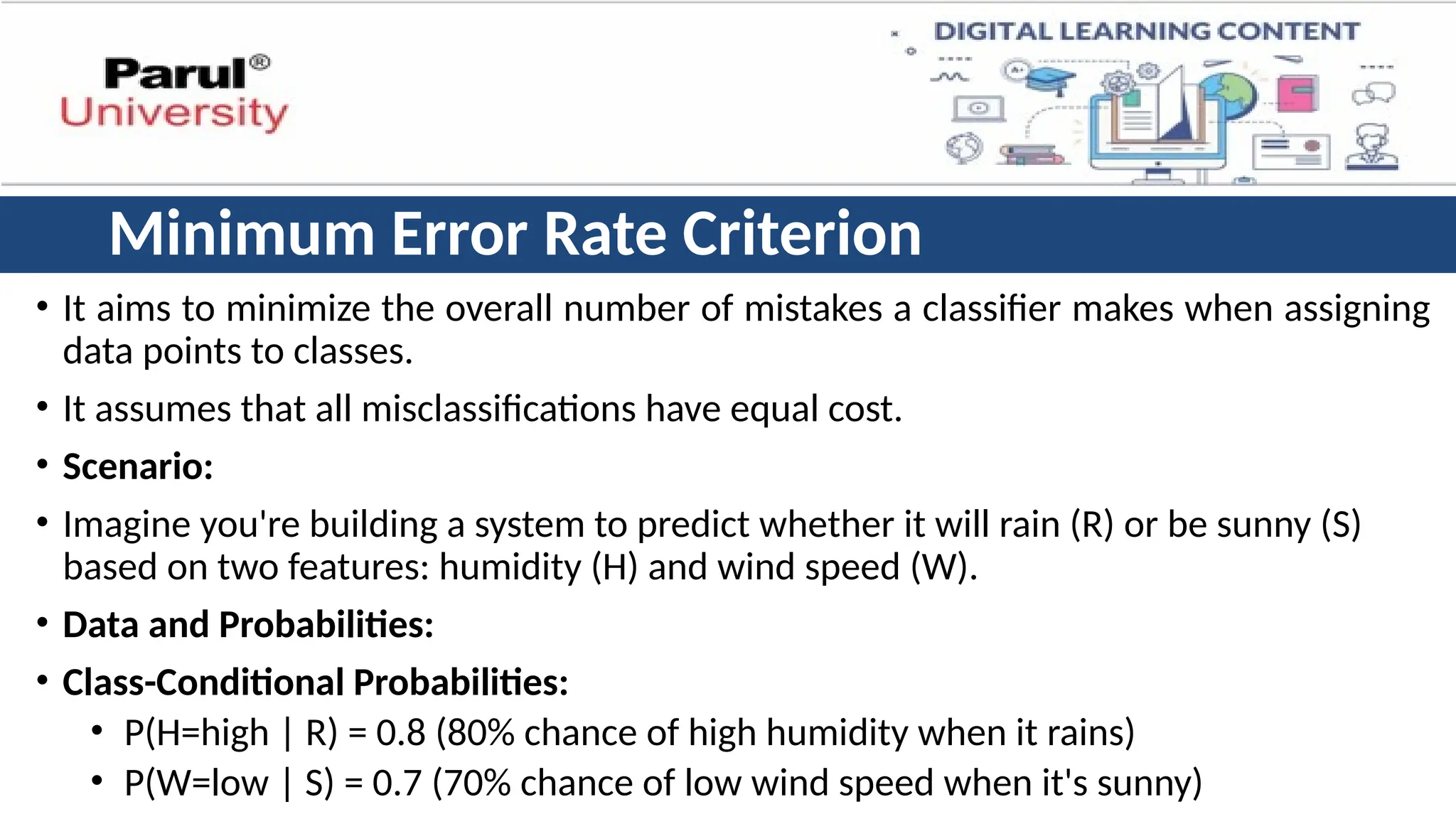
• It aims to minimize the overall number of mistakes a classifier makes when assigning
data points to classes.
• It assumes that all misclassifications have equal cost.
• Scenario:
• Imagine you're building a system to predict whether it will rain (R) or be sunny (S)
based on two features: humidity (H) and wind speed (W).
• Data and Probabilities:
• Class-Conditional Probabilities:
• P(H=high | R) = 0.8 (80% chance of high humidity when it rains)
• P(W=low | S) = 0.7 (70% chance of low wind speed when it's sunny)
81.
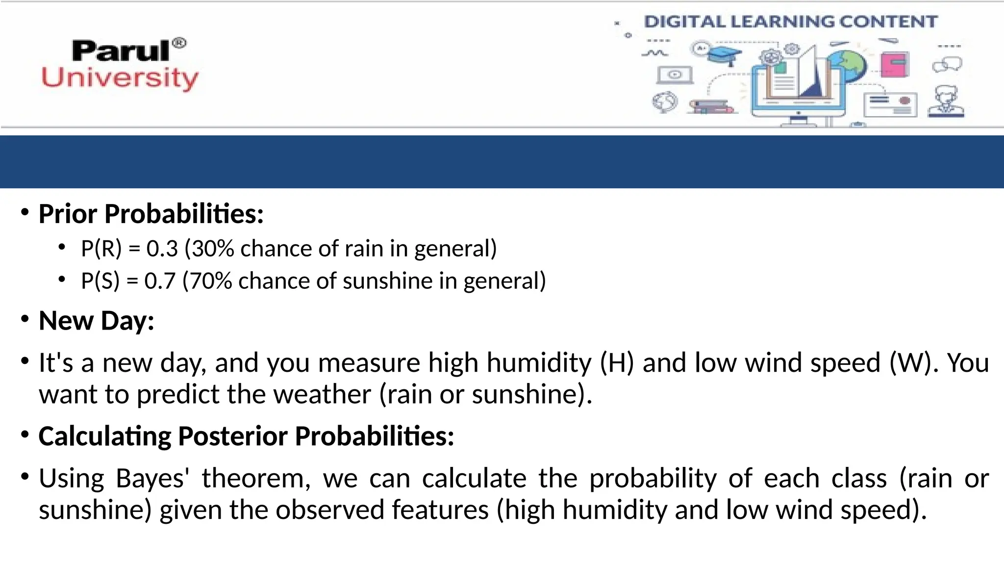
• Prior Probabilities:
•P(R) = 0.3 (30% chance of rain in general)
• P(S) = 0.7 (70% chance of sunshine in general)
• New Day:
• It's a new day, and you measure high humidity (H) and low wind speed (W). You
want to predict the weather (rain or sunshine).
• Calculating Posterior Probabilities:
• Using Bayes' theorem, we can calculate the probability of each class (rain or
sunshine) given the observed features (high humidity and low wind speed).
82.
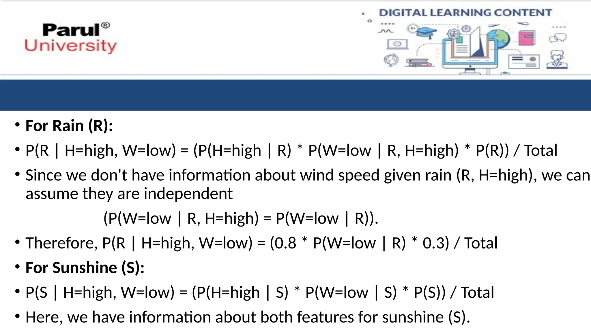
• For Rain(R):
• P(R | H=high, W=low) = (P(H=high | R) * P(W=low | R, H=high) * P(R)) / Total
• Since we don't have information about wind speed given rain (R, H=high), we can
assume they are independent
(P(W=low | R, H=high) = P(W=low | R)).
• Therefore, P(R | H=high, W=low) = (0.8 * P(W=low | R) * 0.3) / Total
• For Sunshine (S):
• P(S | H=high, W=low) = (P(H=high | S) * P(W=low | S) * P(S)) / Total
• Here, we have information about both features for sunshine (S).
83.
• Decision UnderMinimum Error Rate:
• Now, we compare the calculated posterior probabilities for rain (P(R | H=high,
W=low)) and sunshine (P(S | H=high, W=low)).
• If P(R | H=high, W=low) > P(S | H=high, W=low), we predict rain (R) as it has the
higher probability of occurring given the observed features.
• If P(R | H=high, W=low) < P(S | H=high, W=low), we predict sunshine (S).
• Minimizing Error Rate:
• By choosing the class with the highest posterior probability, we minimize the
expected number of incorrect predictions over time.
84.
• Key Points:
•Minimum error rate assumes all misclassifications (predicting rain when it's
sunny or vice versa) have equal cost.
• It works well when classes are well-separated by features (high humidity for
rain, low wind speed for sunshine) and prior probabilities are informative.
• However, the minimum error rate might not be ideal if the cost of
misclassification is not equal.
85.
• Example Limitation:
•Imagine going on a picnic. While a little rain might be manageable, getting
caught in a downpour would ruin the day.
• In this scenario, misclassifying sunshine as rain would be less severe than
vice versa.
• Here, the minimum risk criterion, which considers the cost of
misclassification, might be a better choice.
86.
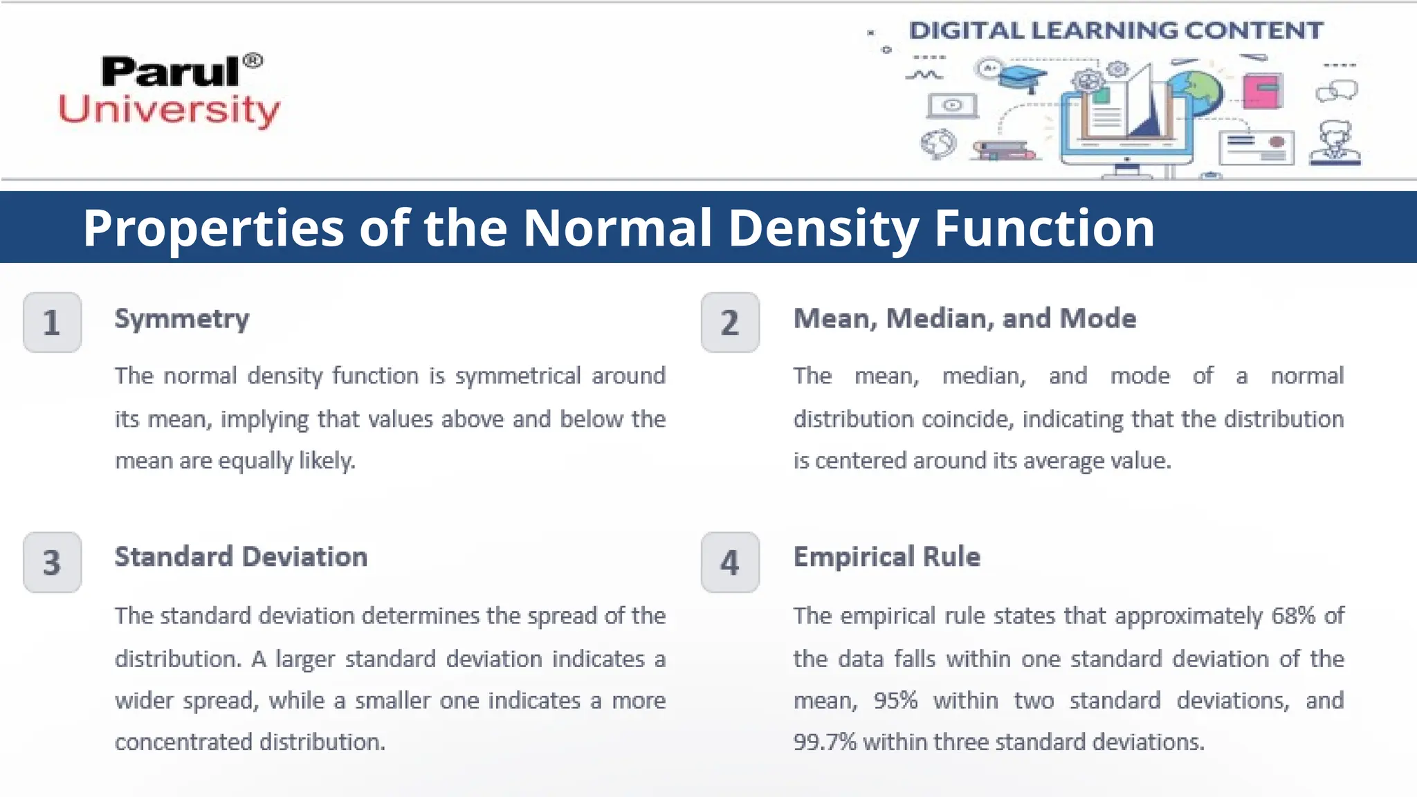
• The normaldensity function, often called the Gaussian distribution, is
a fundamental concept in probability and statistics.
• It describes the probability of a continuous random variable occurring
within a specific range.
• It's characterized by a bell-shaped curve where data points are more
likely to be near the average (mean) and less likely as they deviate
further in either direction.
Normal Density (Gaussian Distribution):
• Key Parameters:
•Mean (μ): Represents the center of the bell curve, indicating the average
value of the data.
• Standard Deviation (σ): Controls the spread of the curve. A larger standard
deviation indicates a wider distribution of data points around the mean.
• Example: Imagine measuring the heights of students in a class.
• The normal density function can model the probability of finding a student
with a specific height.
• Students with heights close to the average class height (mean) will be more
likely, while very short or very tall students will be less likely.
89.
Discriminant Functions inClassification:
• In Bayes' theorem classification, discriminant functions play a crucial
role in separating classes based on their features.
• They utilize the class-conditional probabilities (P(F|C)), which
represent the probability of observing a set of features (F) given a
particular class (C).
• The discriminant function is a mathematical formula that helps classify
observations into different groups based on their characteristics.
• It assigns a score to each observation, and the group with the highest
score is chosen as the most likely classification.
Types of DiscriminantFunctions:
1. Linear Discriminant Function (LDF)
2. Non-Linear (Quadratic) Discriminant Function
92.
Linear Discriminant Function(LDF)
• This function is a linear combination of the features, often used when the
class-conditional probabilities follow a normal distribution with equal
covariance matrices.
• It takes the form:
• g(x) = w^T * x + b
where:
• g(x) is the discriminant score for class C
• w is a weight vector learned from the data
• x is the feature vector of a new data point
• b is a bias term
93.
Non-Linear (Quadratic) DiscriminantFunction
• When the class-conditional distributions are not well-represented by
a single normal distribution or the covariance matrices are different,
non-linear functions might be used.
• The non linear or quadratic discriminant function provides a more
flexible approach, allowing for non-linear decision boundaries.
• It uses a quadratic equation to compute the discriminant score.
• Examples include polynomial functions, support vector machines
(SVMs), or neural networks.
94.
• Discriminant functionsare often used in conjunction with Bayes'
theorem to make classification decisions. Here's how:
1.We calculate the posterior probability (P(C|F)) for each class using
Bayes' theorem.
2.We utilize the class-conditional probabilities (P(F|C)) within the
discriminant function to represent these probabilities.
3.We compare the discriminant scores (g(x)) for each class, which
effectively capture the posterior probabilities based on the features.
4.We assign the new data point to the class with the highest discriminant
score (or highest posterior probability).
95.
• Example:
• Continuingfrom the handwritten digit classification example, an LDF
could be used to separate the classes.
• By calculating the discriminant score for each digit class based on the
features (pixel intensities), we can classify a new handwritten digit into
the class with the highest score.
• Normal density helps model the distribution of features within each
class, while discriminant functions leverage these class-conditional
probabilities to separate classes and make optimal classification
decisions using Bayes' theorem.
96.
• Imagine you'resorting fruits at a grocery store.
• You want to separate oranges from apples, but they're all mixed up in a
bin.
• Discriminant functions are like special rules you can use to make this
sorting process faster and more accurate.
• Here's how it works:
1.Fruit Features: You consider two main features of the fruits: weight
(heavy or light) and color (red or orange).
97.
2. Discriminant Function:This function is like a decision-making rule
based on these features.
It could be something simple like: "If the fruit is heavy AND red, classify
it as an apple; otherwise, classify it as an orange." This is a very basic
example, and more complex functions can be used in real-world
scenarios.
Benefits of Discriminant Functions:
• Faster Sorting: By using the discriminant function, you can quickly
decide which basket to put each fruit in based on its weight and color.
You don't have to spend time carefully examining every single fruit.
98.
• Reduced Errors:Having a clear rule helps you avoid mistakes. You're
less likely to accidentally put an orange in the apple basket (or vice
versa).
Limitations:
• Oversimplification: This example uses a simple function with clear-cut
rules. In real life, fruits might have more variations in color and weight,
and the discriminant function might need to be more complex to handle
these variations.
• Not Perfect: There might still be some errors, especially for fruits that
fall on the edge (e.g., a very light, slightly reddish apple).
99.
Decision Surfaces –Visualizing Classification Boundary
• Decision surfaces are a fundamental concept in classification tasks within machine
learning.
• They offer a visual representation of how a classification model separates different
classes based on their features by using discriminant functions.
Building Blocks of Decision Surfaces:
• Features: These are the characteristics used to describe and differentiate data
points. In our fruit sorting example, size and weight were the features.
• Data Points: Each data point represents an individual instance you want to
classify. It's characterized by its feature values.
• Classification Model: This is the algorithm that learns to categorize data points
based on their features.
100.
Difference between Decisionboundary and Decision surfaces
• Decision Boundary (Lower Dimensions): In simple classification
problems with two features, a decision boundary is a line in a two-
dimensional space that separates the classes.
• Imagine separating apples and oranges based on size and weight.
• It is also known as linear decision surface.
• Decision Surface (Higher Dimensions): In problems with more than two
features, the decision boundary becomes a higher-dimensional surface.
• It separates the feature space into regions, where each region corresponds
to a specific class. This surface is called the decision surface.
• It is also known as non - linear decision surface.
101.
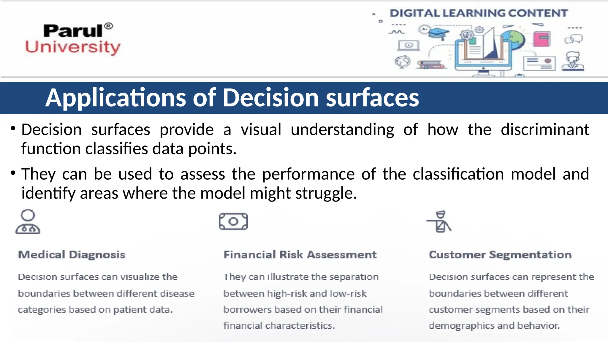
Applications of Decisionsurfaces
• Decision surfaces provide a visual understanding of how the discriminant
function classifies data points.
• They can be used to assess the performance of the classification model and
identify areas where the model might struggle.
102.
Parameter estimation
• Parameterestimation is a fundamental aspect of statistical modeling,
involving the process of determining the values of unknown parameters
within a statistical model.
• This process is crucial for understanding and interpreting data, allowing us to
draw inferences and make predictions.
• Parameter estimation is the process of finding the values of unknown
parameters in a model that best fit the observed data.
103.
Maximum Likelihood estimationmethod
• MLE aims to find the parameter values that maximize the likelihood of
observing the actual data.
• In simpler terms, it estimates the parameters that make the observed
data most probable given the model.
Advantages:
• Widely used and efficient for many models.
• Provides a single "best" estimate for each parameter.
Disadvantages:
• Sensitive to outliers in the data.
• May not perform well with small datasets or complex models.
Properties of MLE
•Asymptotic Consistency 🡪 As the sample size grows, MLE estimates converge
to the true parameter values.
• Asymptotic Efficiency🡪 MLE estimates have the lowest possible variance
among all consistent estimators under certain conditions.
• Asymptotic Normality 🡪MLE estimates are asymptotically normally
distributed, allowing for the construction of confidence intervals and hypothesis
testing.
106.
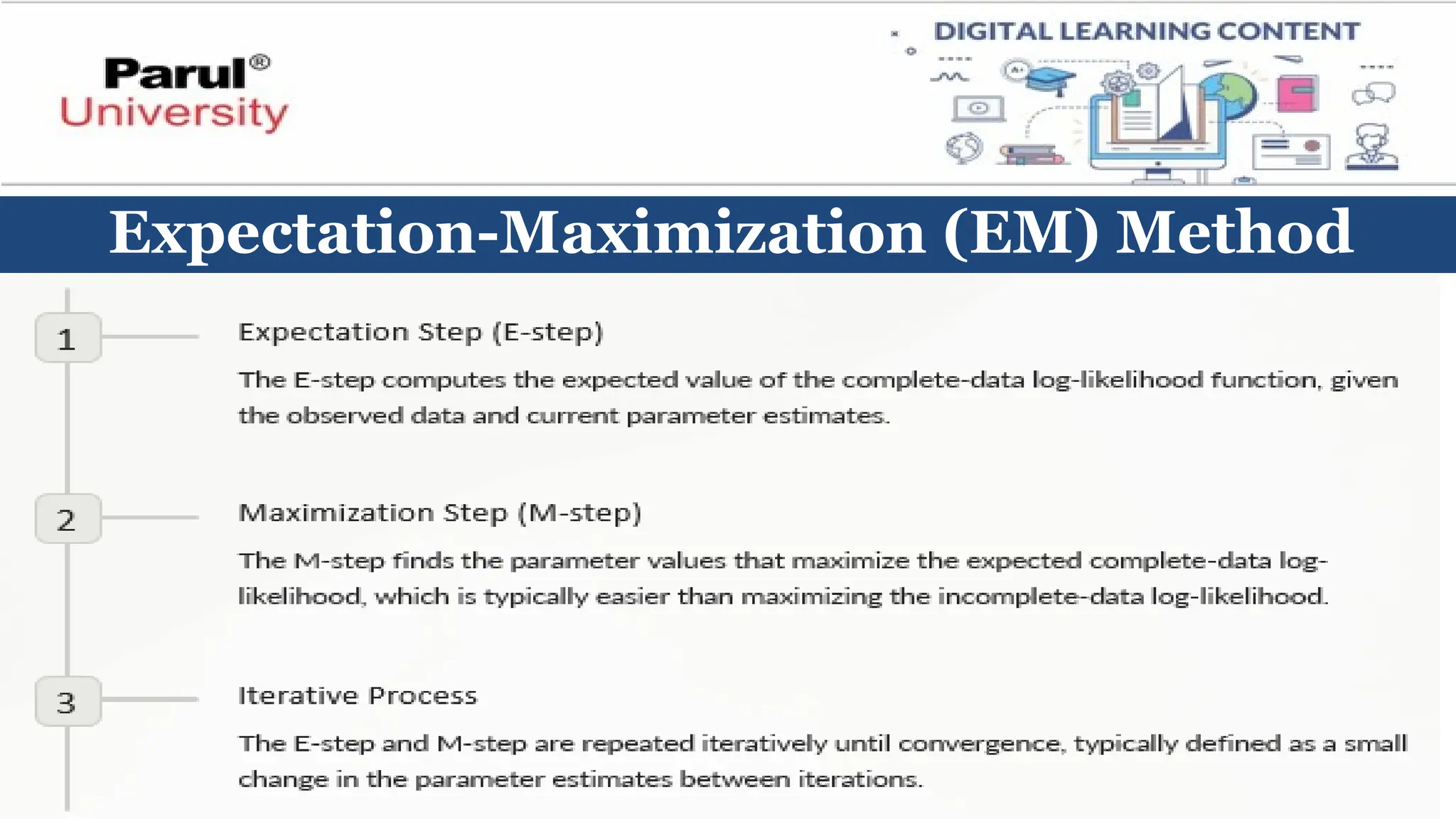
Expectation-Maximization (EM) Method
•The EM algorithm is an iterative approach used to estimate parameters
in models with latent variables.
• Latent variables are hidden or unobserved variables that influence the
observed data.
Process
1.Define a model with observed data and latent variables. (e.g., model for
customer segmentation with hidden buying habits)
2.Initialize the parameter values with educated guesses.
Advantages:
• Capable ofhandling models with latent variables.
• Often converges well even with complex models.
Disadvantages:
• Requires careful initialization of parameters.
• Convergence can be slow in some cases.
109.
Bayesian Parameter Estimation
•This approach incorporates prior knowledge or beliefs about the
parameters into the estimation process.
• It uses Bayes' theorem to calculate the posterior distribution of the
parameters, which represents the probability of the parameters given
the observed data and prior knowledge.
110.
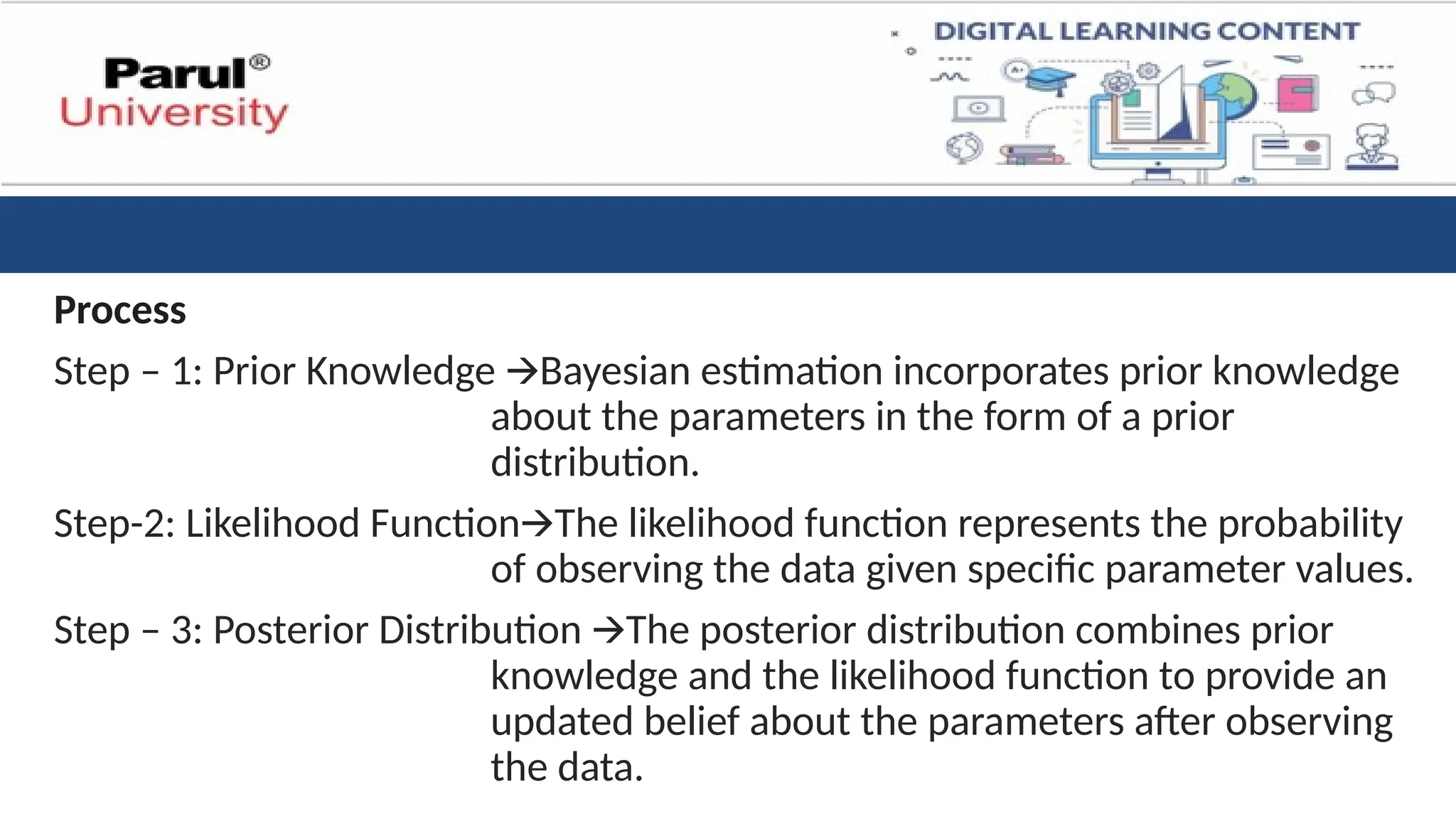
Process
Step – 1:Prior Knowledge Bayesian estimation incorporates prior knowledge
🡪
about the parameters in the form of a prior
distribution.
Step-2: Likelihood Function The likelihood function represents the probability
🡪
of observing the data given specific parameter values.
Step – 3: Posterior Distribution The posterior distribution combines prior
🡪
knowledge and the likelihood function to provide an
updated belief about the parameters after observing
the data.
111.
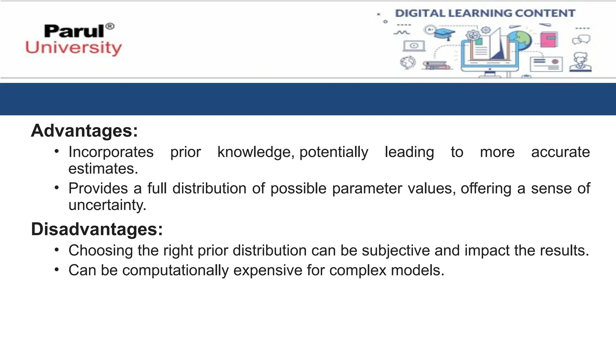
Advantages:
• Incorporates priorknowledge, potentially leading to more accurate
estimates.
• Provides a full distribution of possible parameter values, offering a sense of
uncertainty.
Disadvantages:
• Choosing the right prior distribution can be subjective and impact the results.
• Can be computationally expensive for complex models.
112.
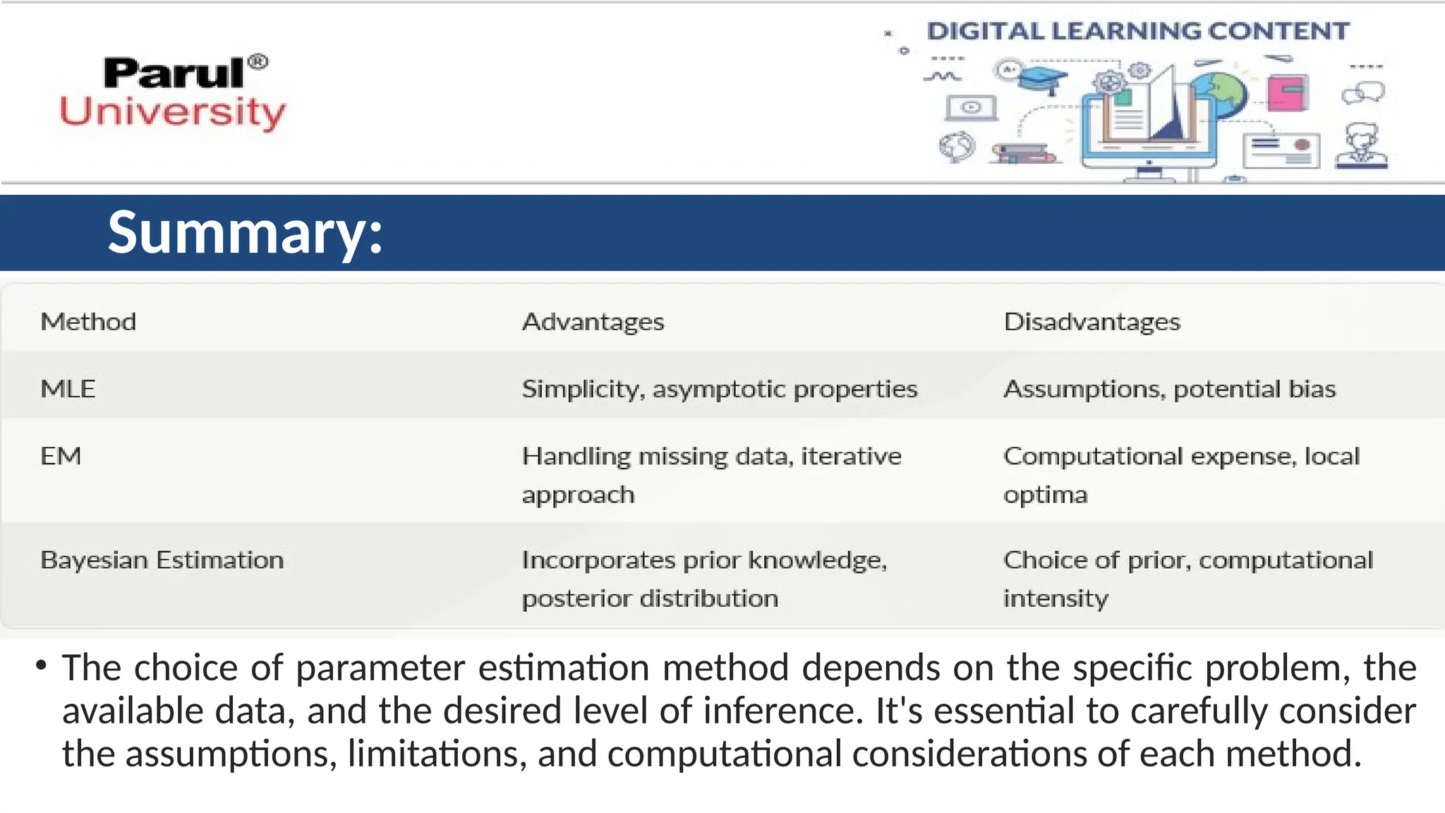
Summary:
• The choiceof parameter estimation method depends on the specific problem, the
available data, and the desired level of inference. It's essential to carefully consider
the assumptions, limitations, and computational considerations of each method.


![Standard Deviation (σ):
• The Standard Deviation is a measure of how spread out numbers are.
• This signifies the spread of the data around the mean.
• There are two common ways to calculate standard deviation,
(i) depending on whether you want the population standard deviation (σ)
reflecting the entire population, or
(ii) the sample standard deviation (s) reflecting a specific sample:
1. Population Standard Deviation (σ):
σ = √[Σ (x - μ)² / n]
ᵢ](https://image.slidesharecdn.com/unit1-1-250824082423-94db5acf/75/Image-processing-technology-and-introduction-60-2048.jpg)
![s = √[Σ (xᵢ - μ)² / (n - 1)]
• where:
• s is the sample standard deviation
• μ (mu) is the mean (as calculated earlier)
• xᵢ (x subscript i) represents each individual data point
• Σ (sigma) denotes summation over all data points (i = 1 to n)
• n is the total number of data points](https://image.slidesharecdn.com/unit1-1-250824082423-94db5acf/75/Image-processing-technology-and-introduction-63-2048.jpg)


![Standard Deviation (σ):
• The Standard Deviation is a measure of how spread out numbers are.
• This signifies the spread of the data around the mean.
• There are two common ways to calculate standard deviation,
(i) depending on whether you want the population standard deviation (σ)
reflecting the entire population, or
(ii) the sample standard deviation (s) reflecting a specific sample:
1. Population Standard Deviation (σ):
σ = √[Σ (x - μ)² / n]
ᵢ](https://crownmelresort.com/image.slidesharecdn.com/unit1-1-250824082423-94db5acf/75/Image-processing-technology-and-introduction-60-2048.jpg)


![s = √[Σ (xᵢ - μ)² / (n - 1)]
• where:
• s is the sample standard deviation
• μ (mu) is the mean (as calculated earlier)
• xᵢ (x subscript i) represents each individual data point
• Σ (sigma) denotes summation over all data points (i = 1 to n)
• n is the total number of data points](https://crownmelresort.com/image.slidesharecdn.com/unit1-1-250824082423-94db5acf/75/Image-processing-technology-and-introduction-63-2048.jpg)