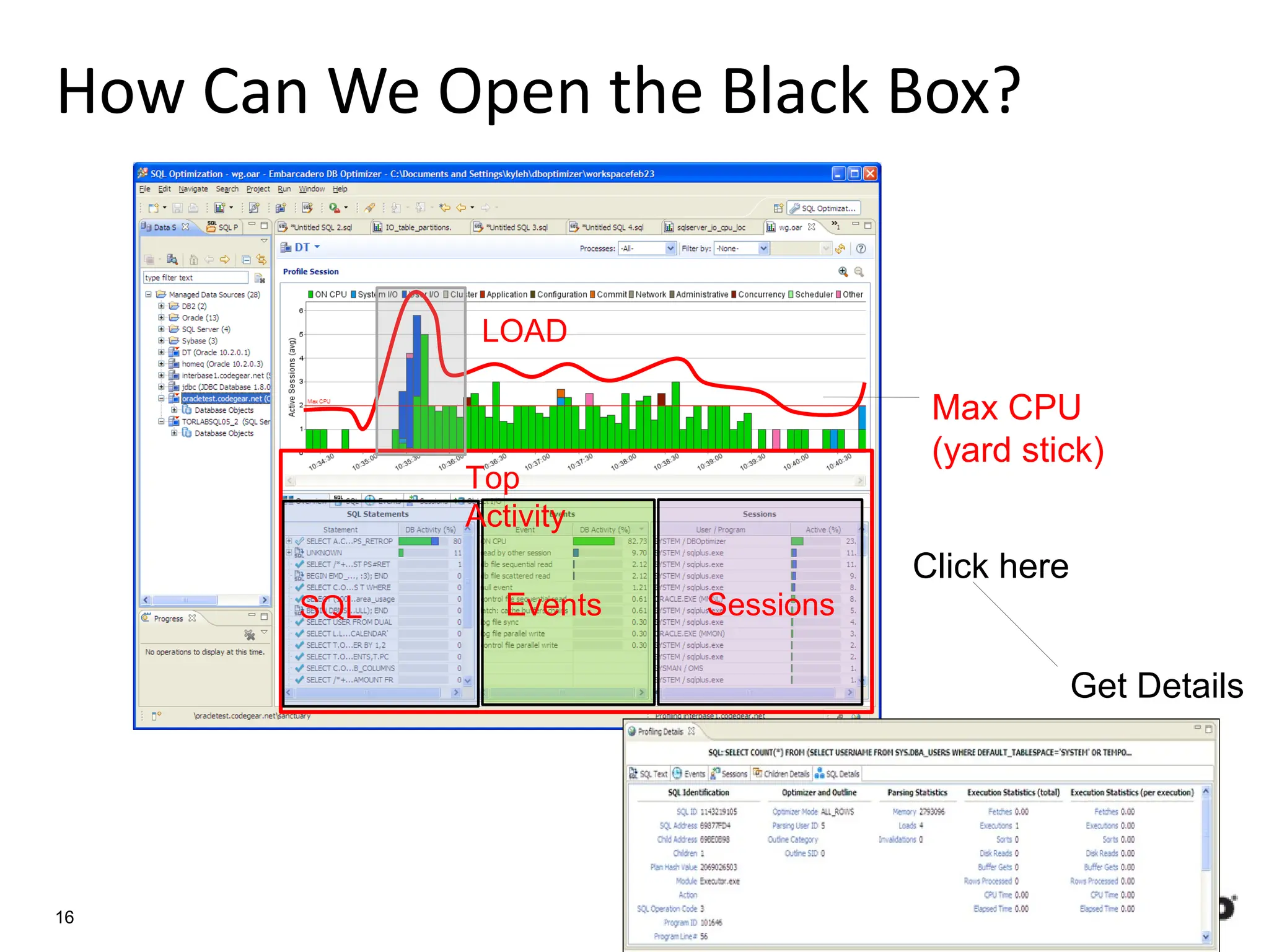
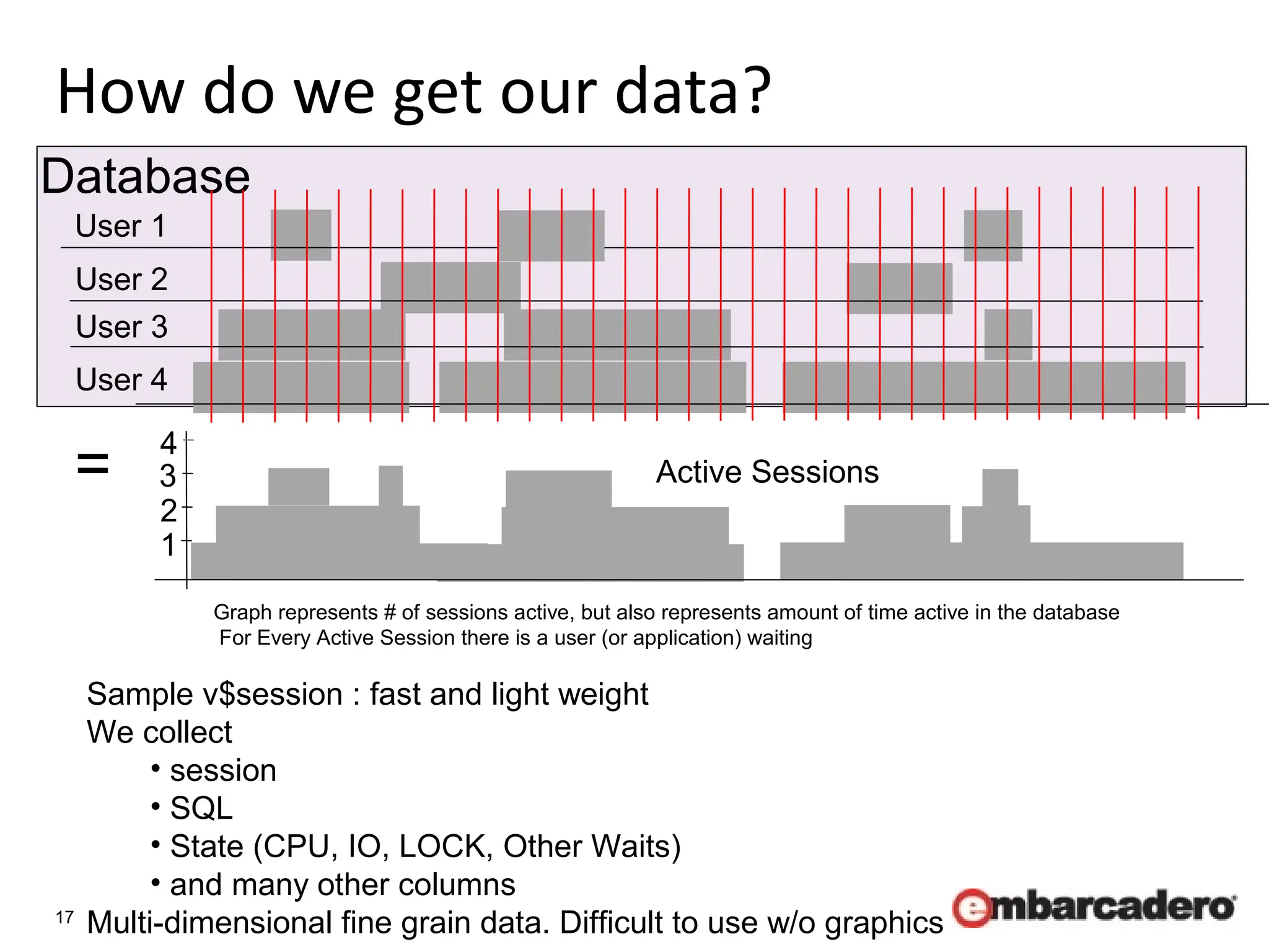
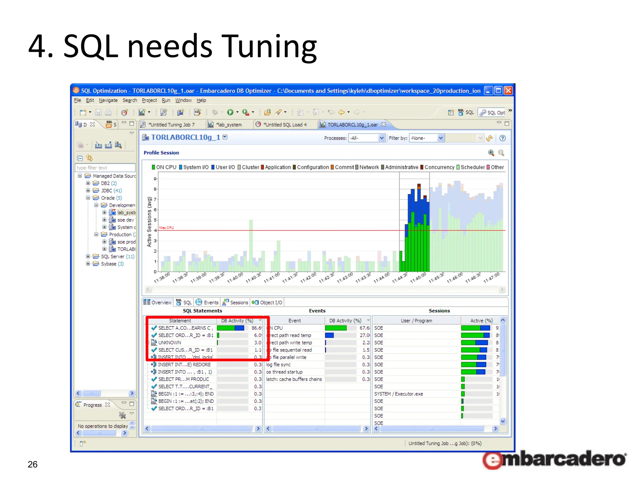
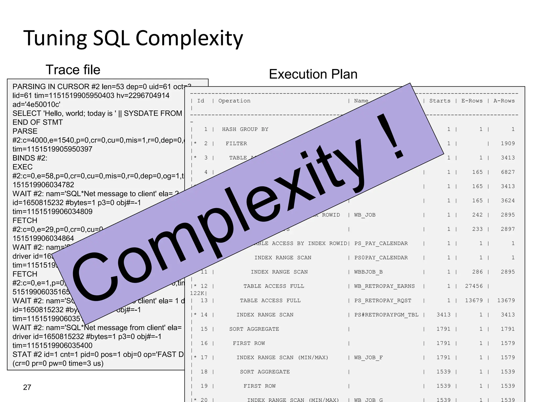
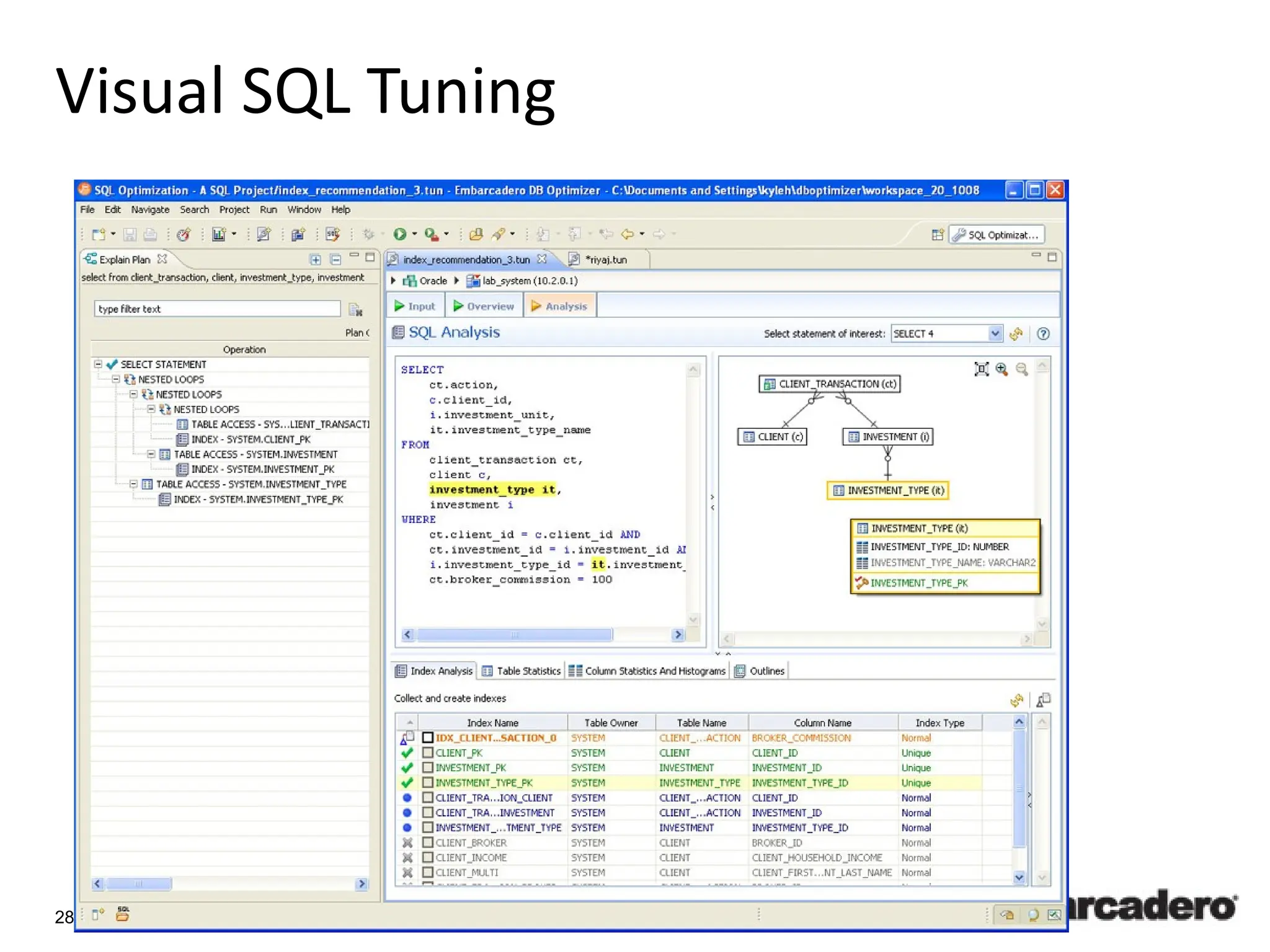
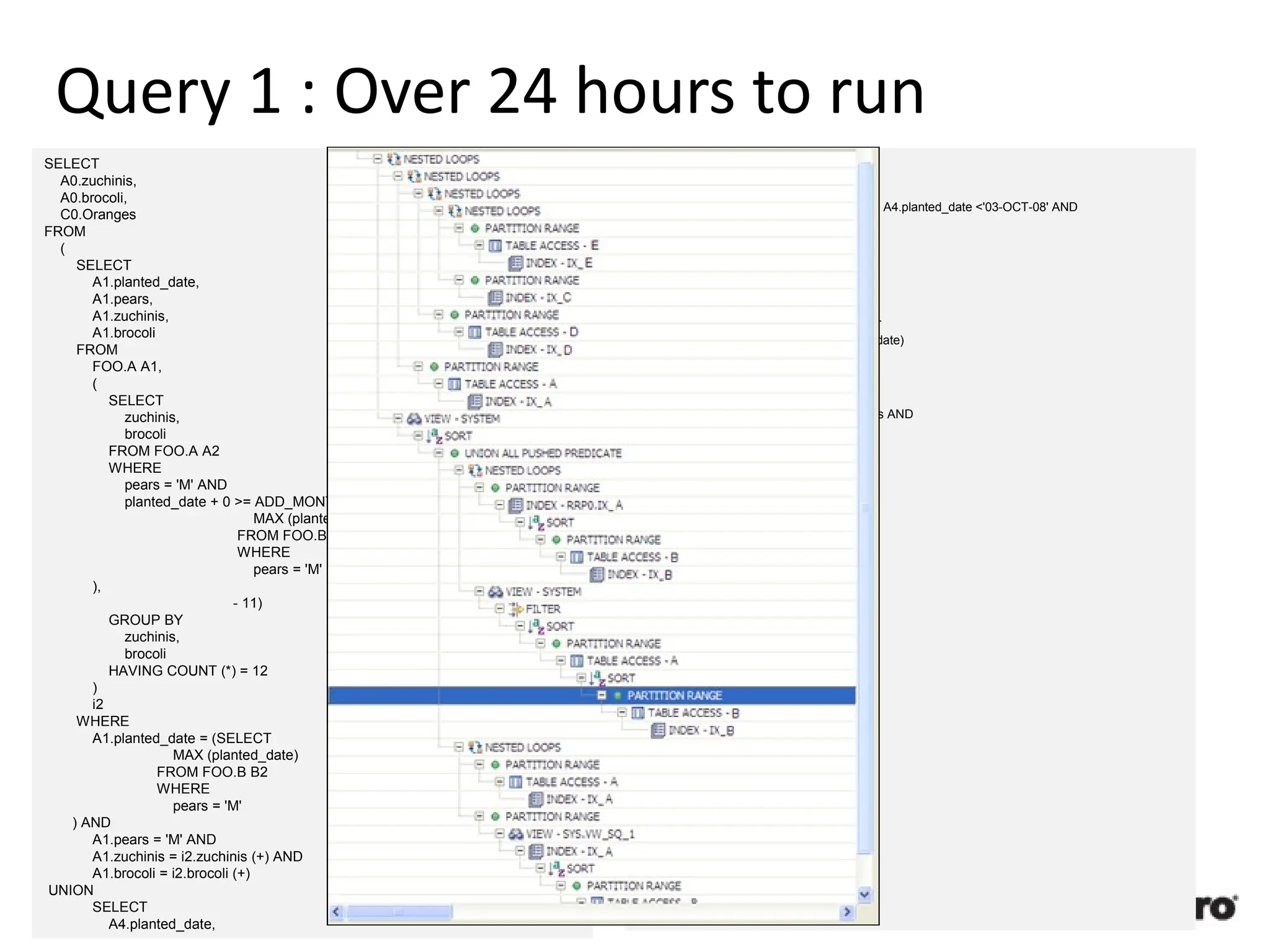
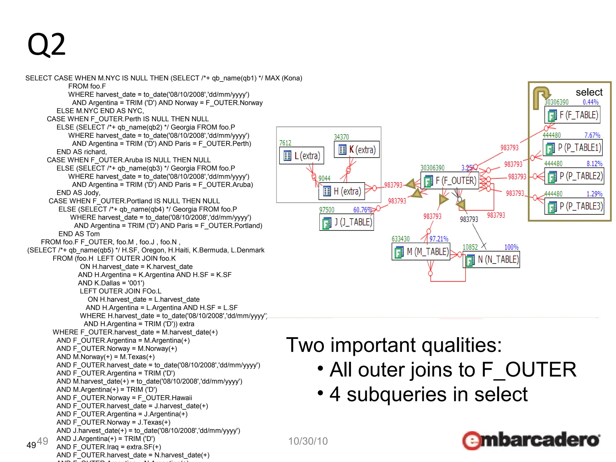
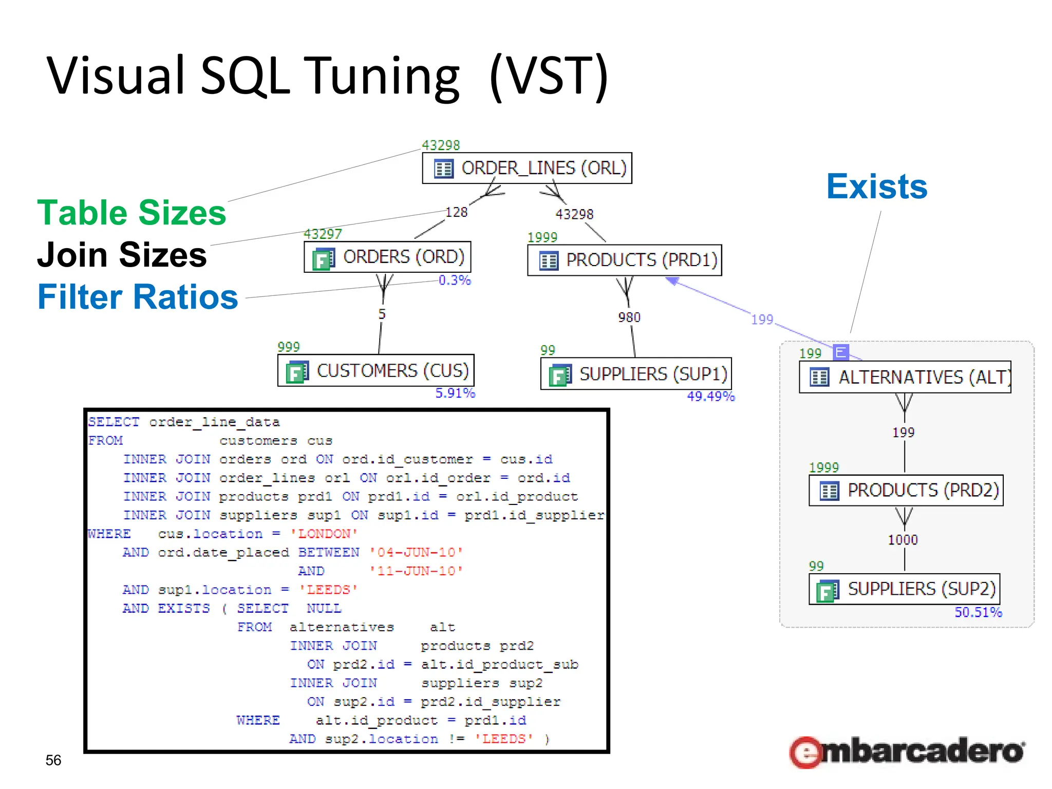
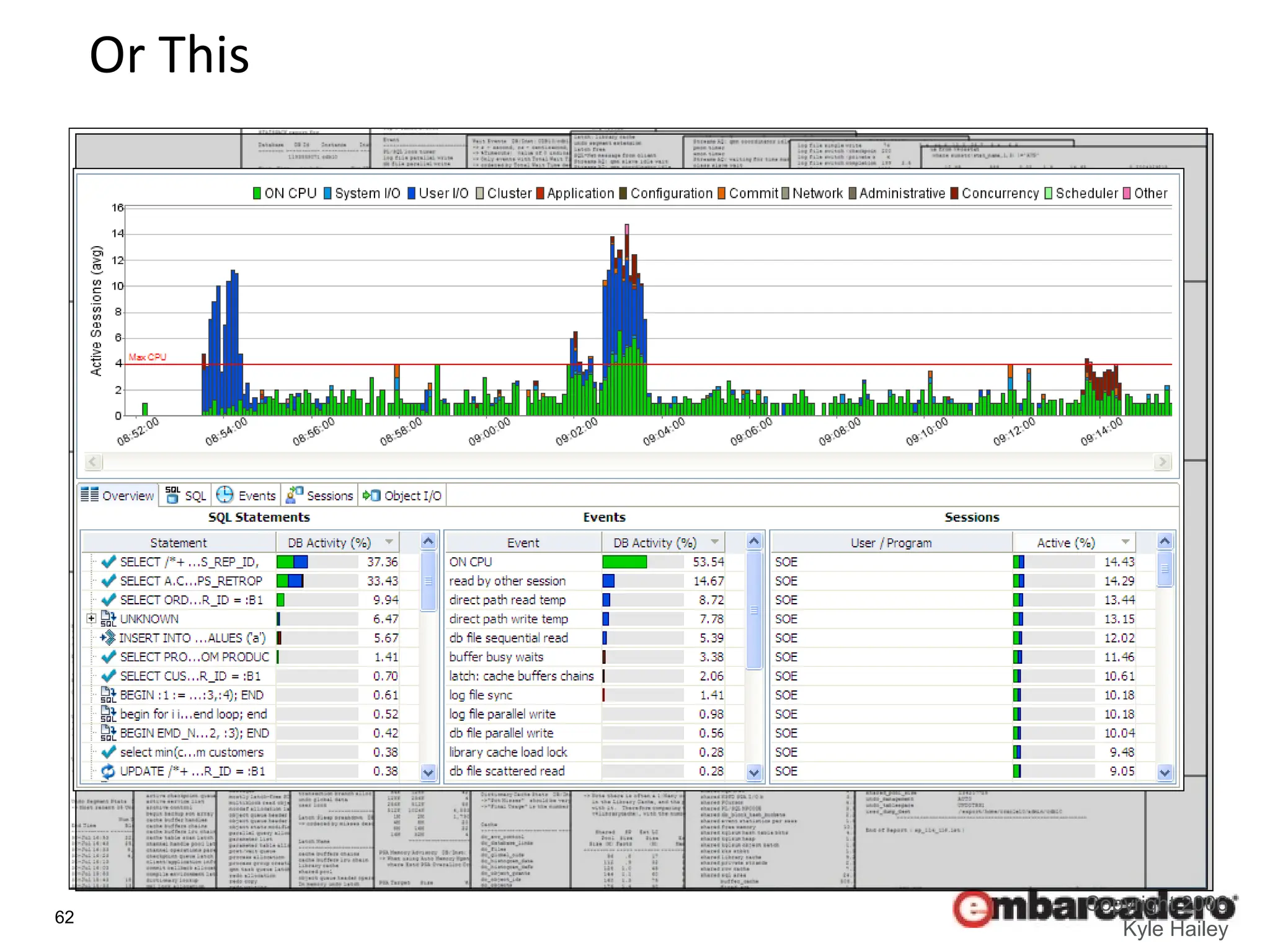
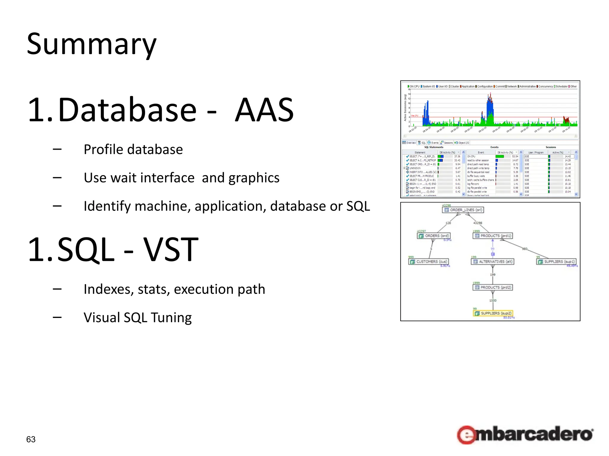
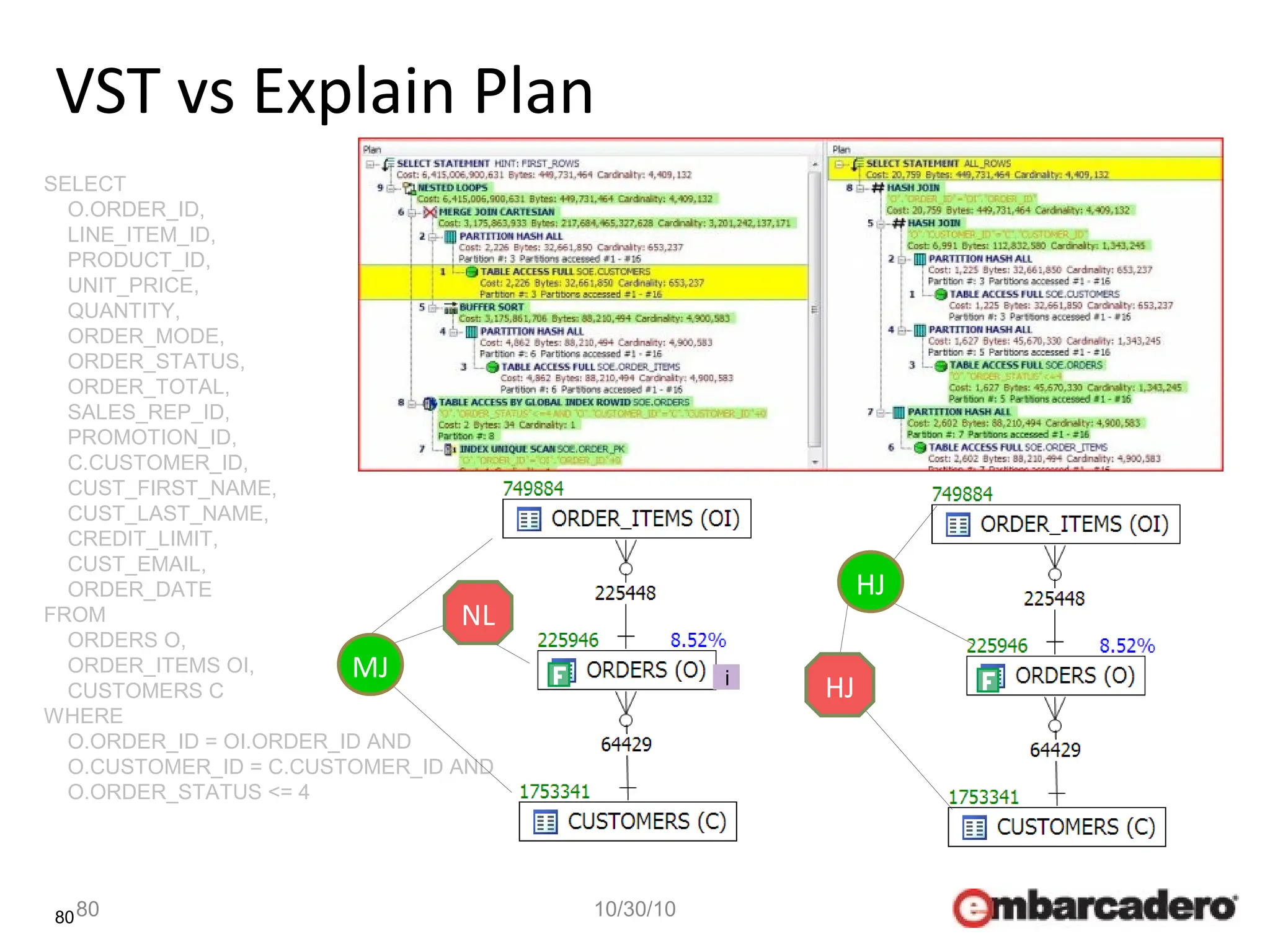
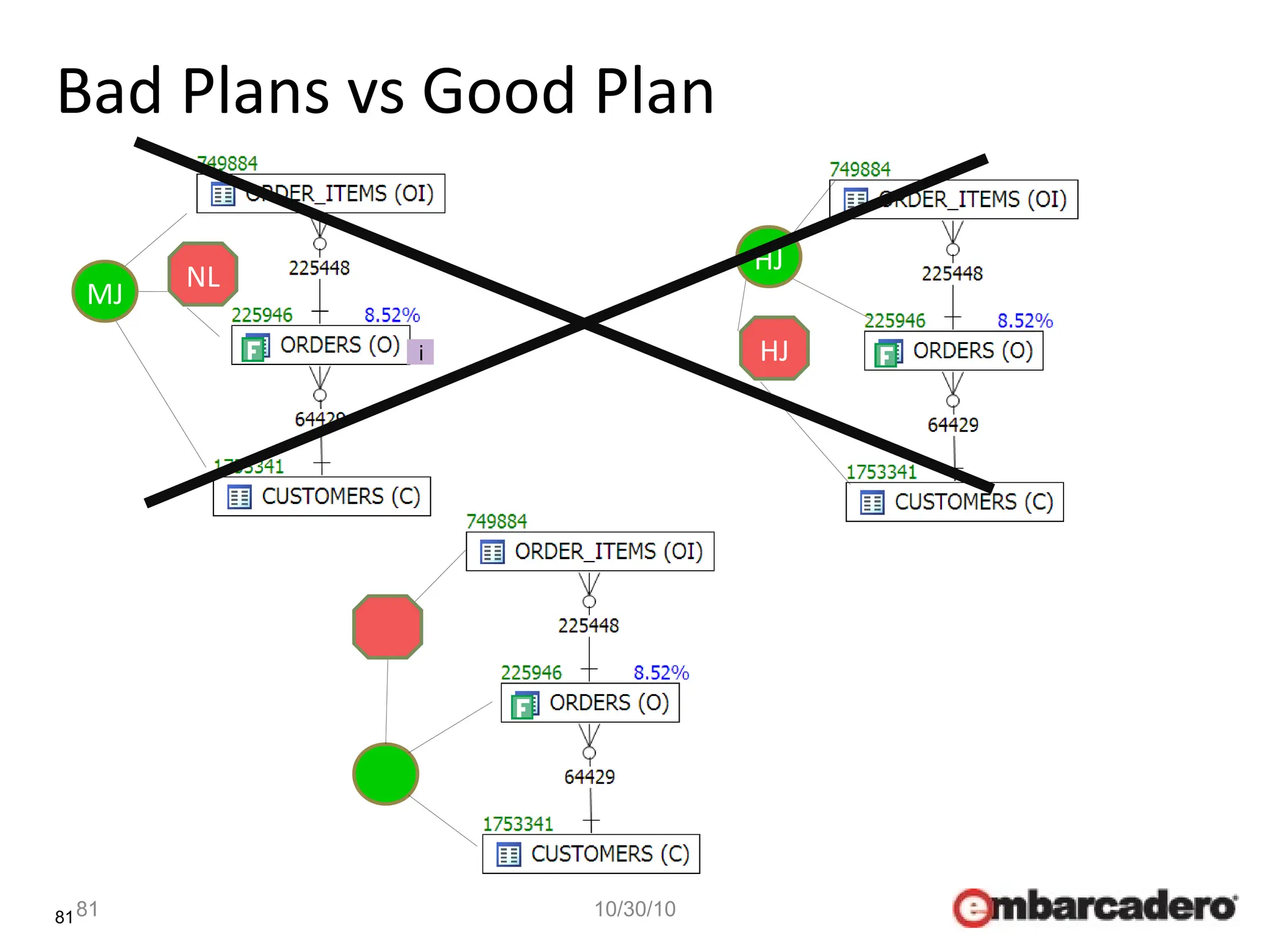
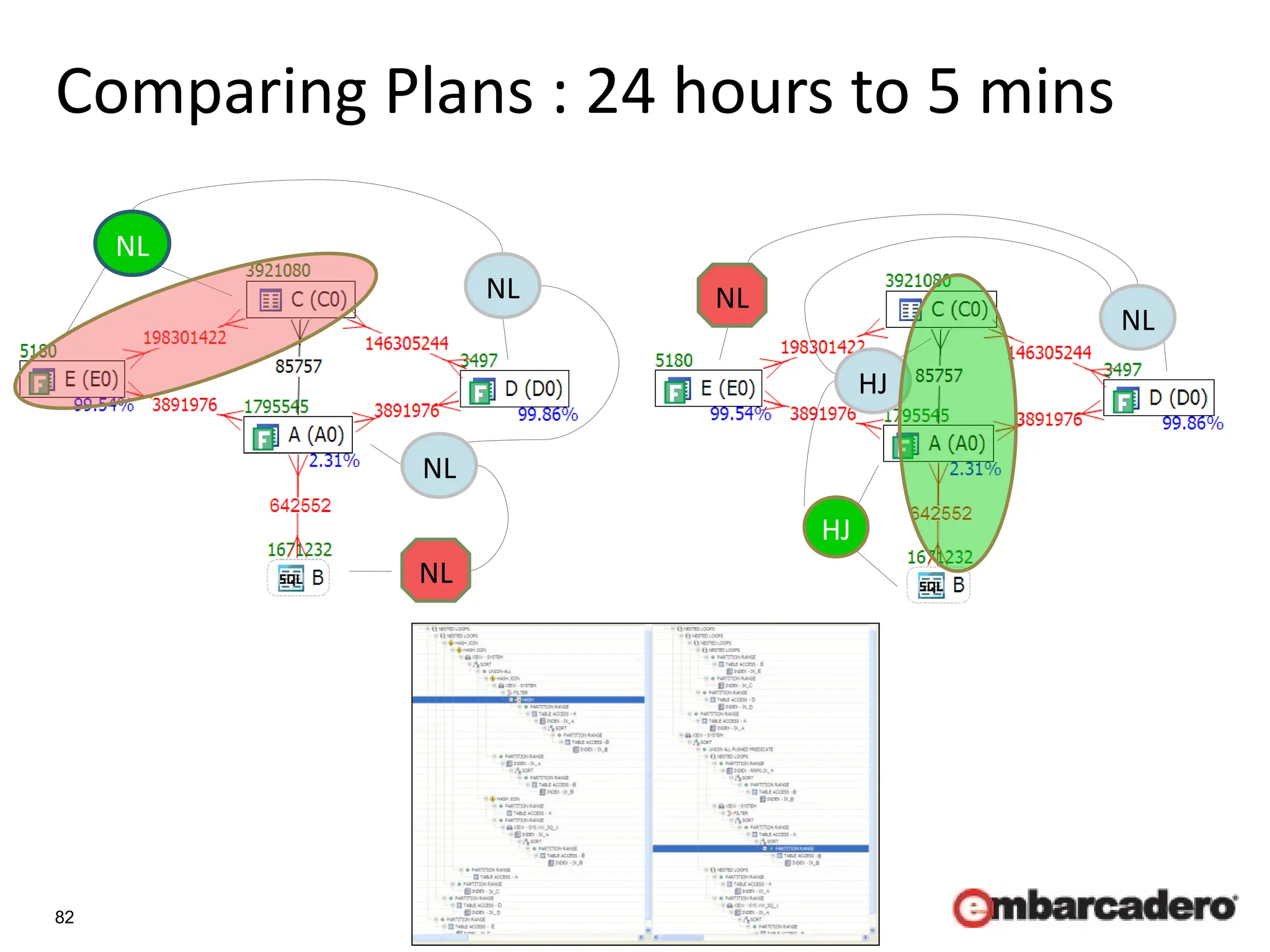
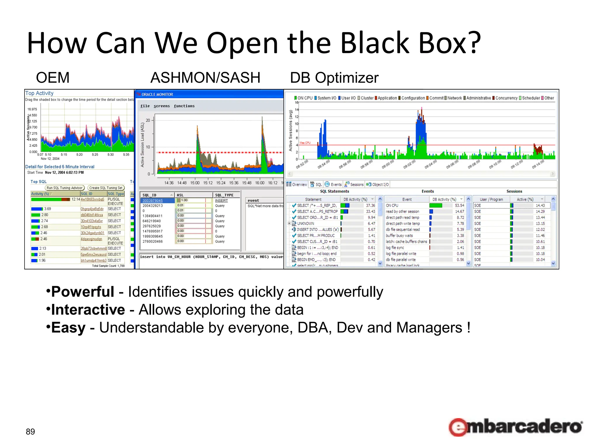
1. The document discusses using graphics and data visualization to improve understanding of database performance issues and SQL tuning. It provides examples of how visualizations can clearly show relationships in complex SQL queries and data that are difficult to understand from text or code alone.
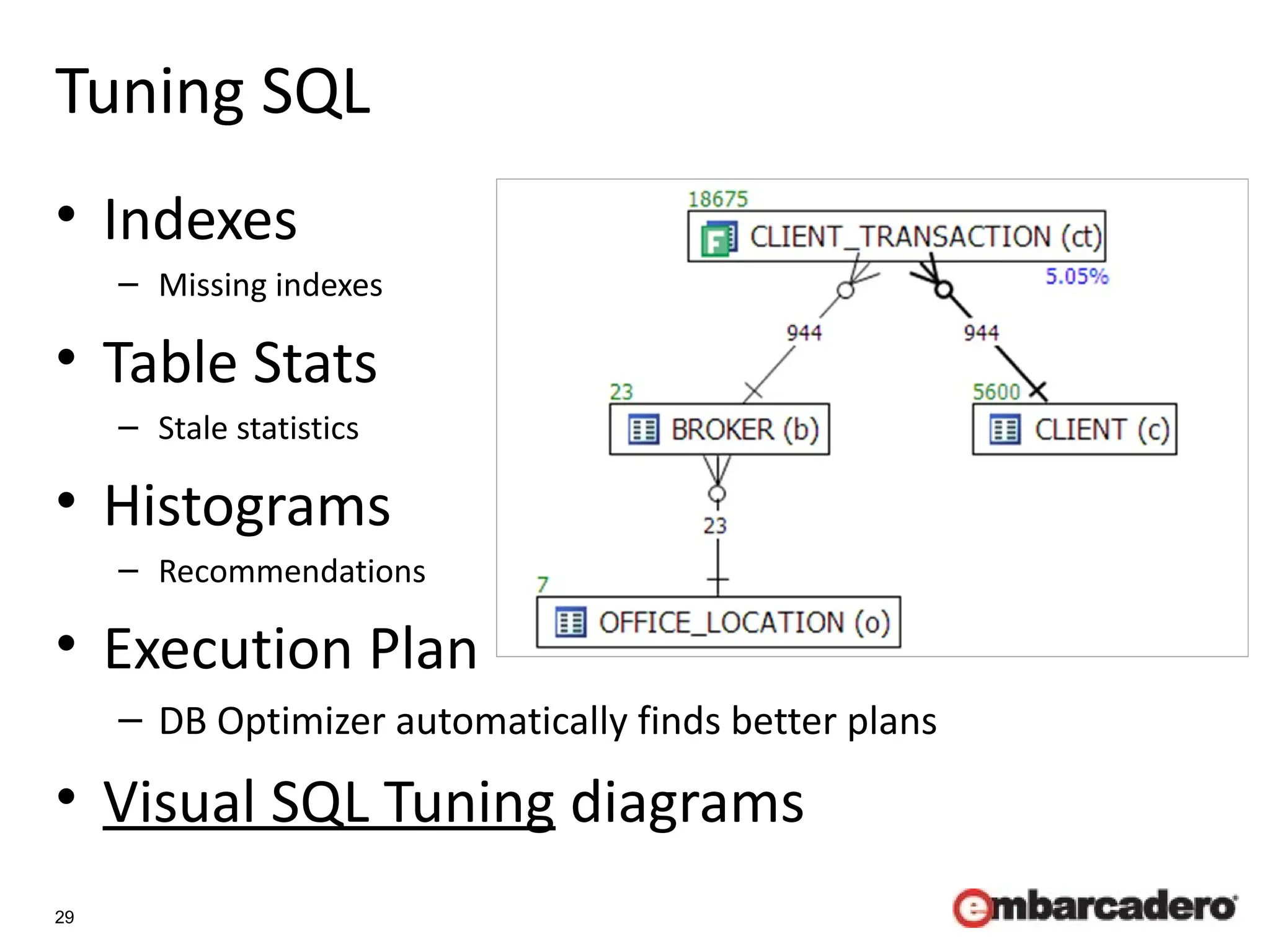
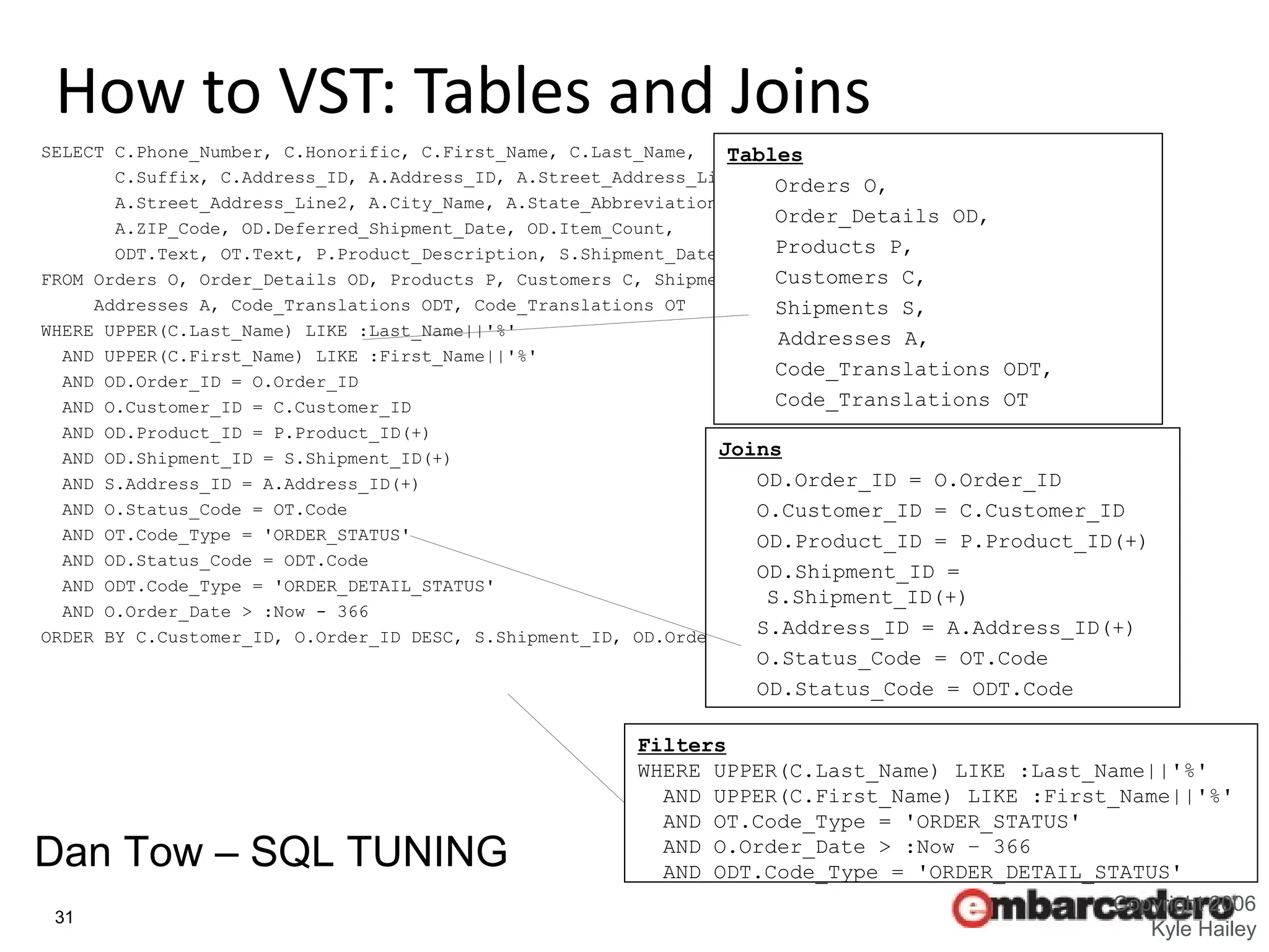
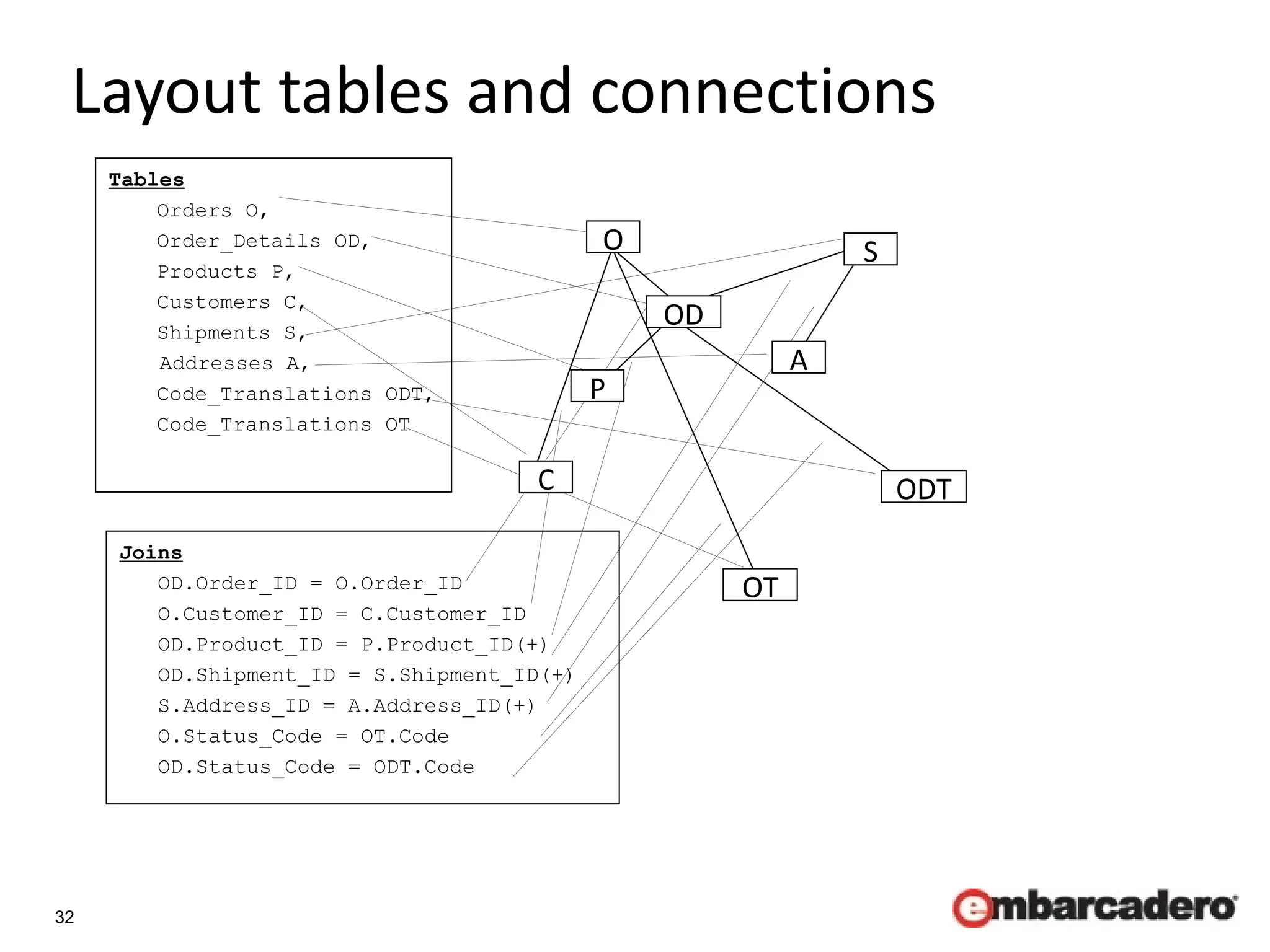
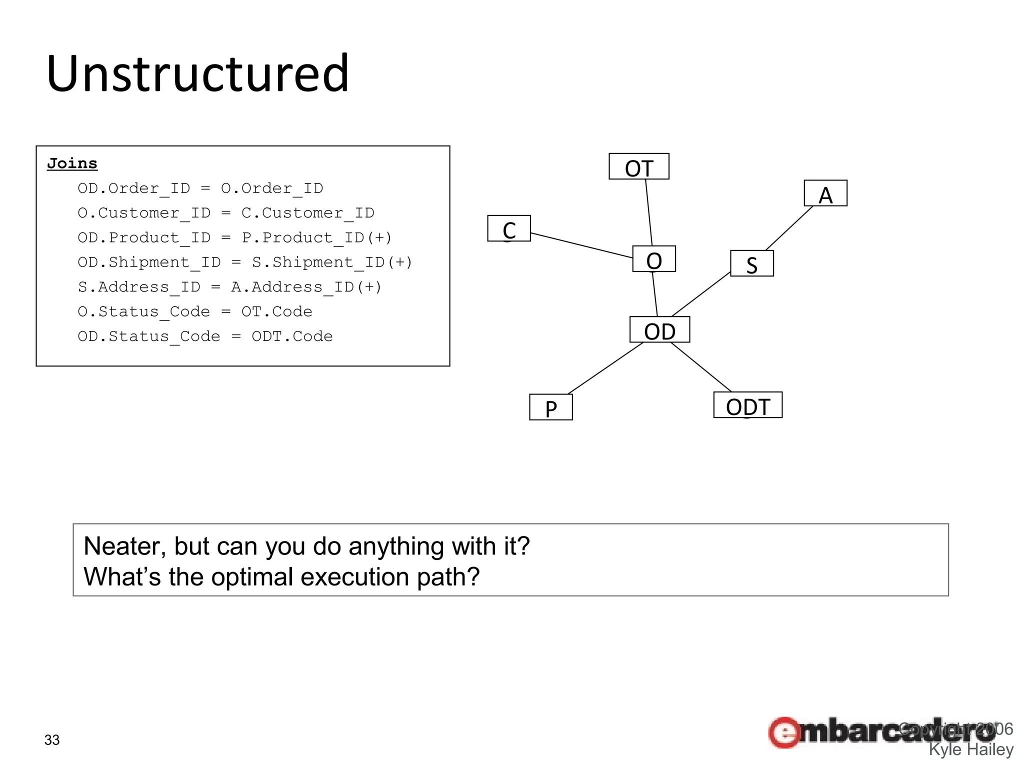
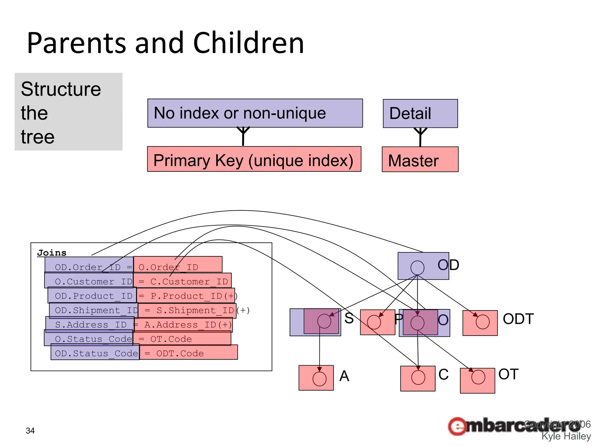
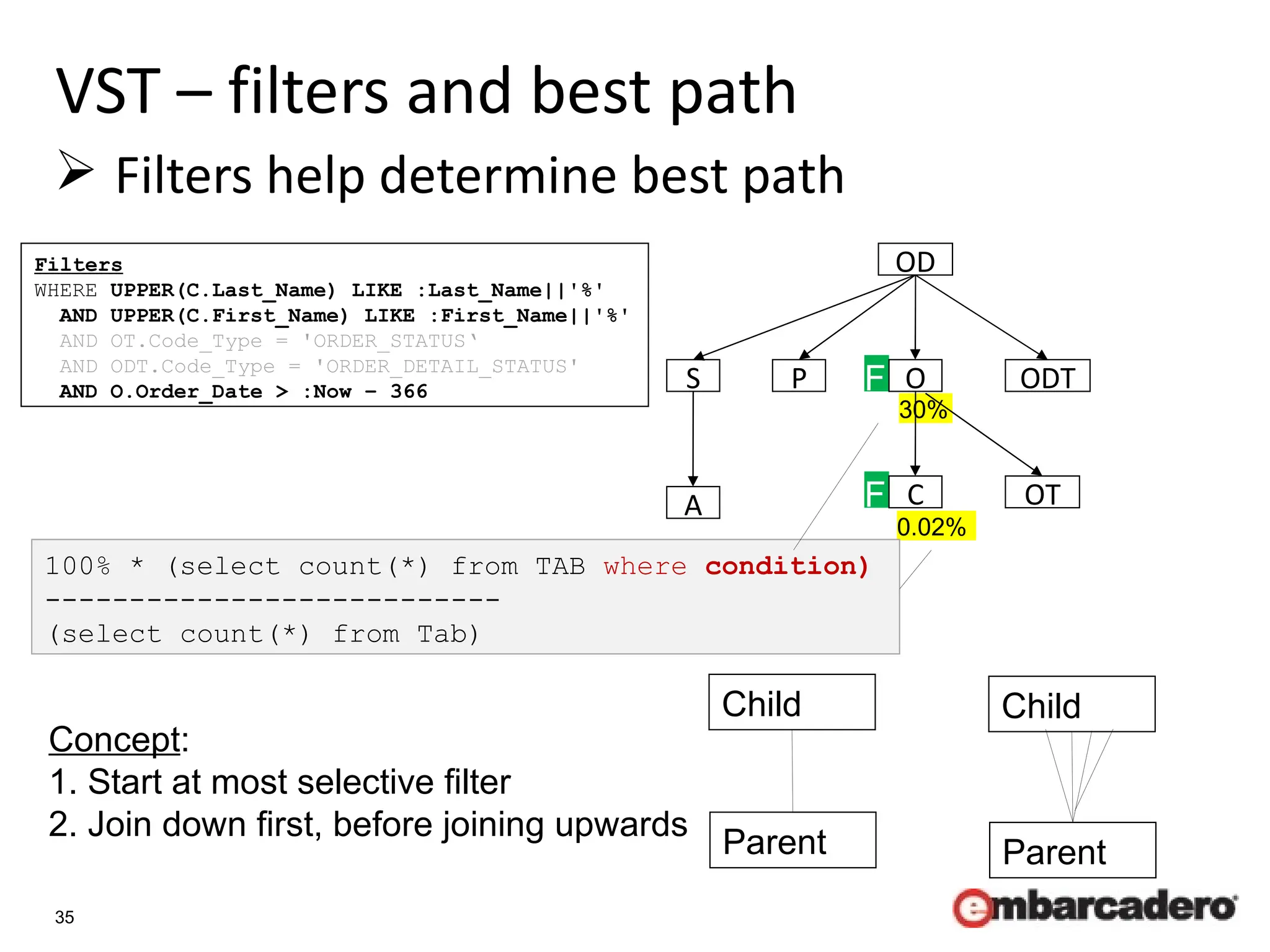
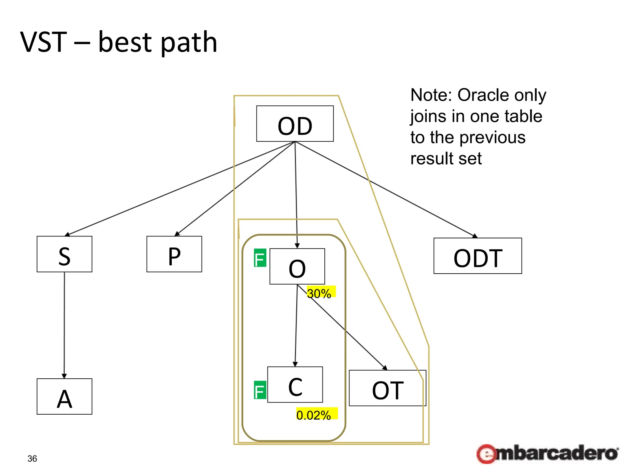
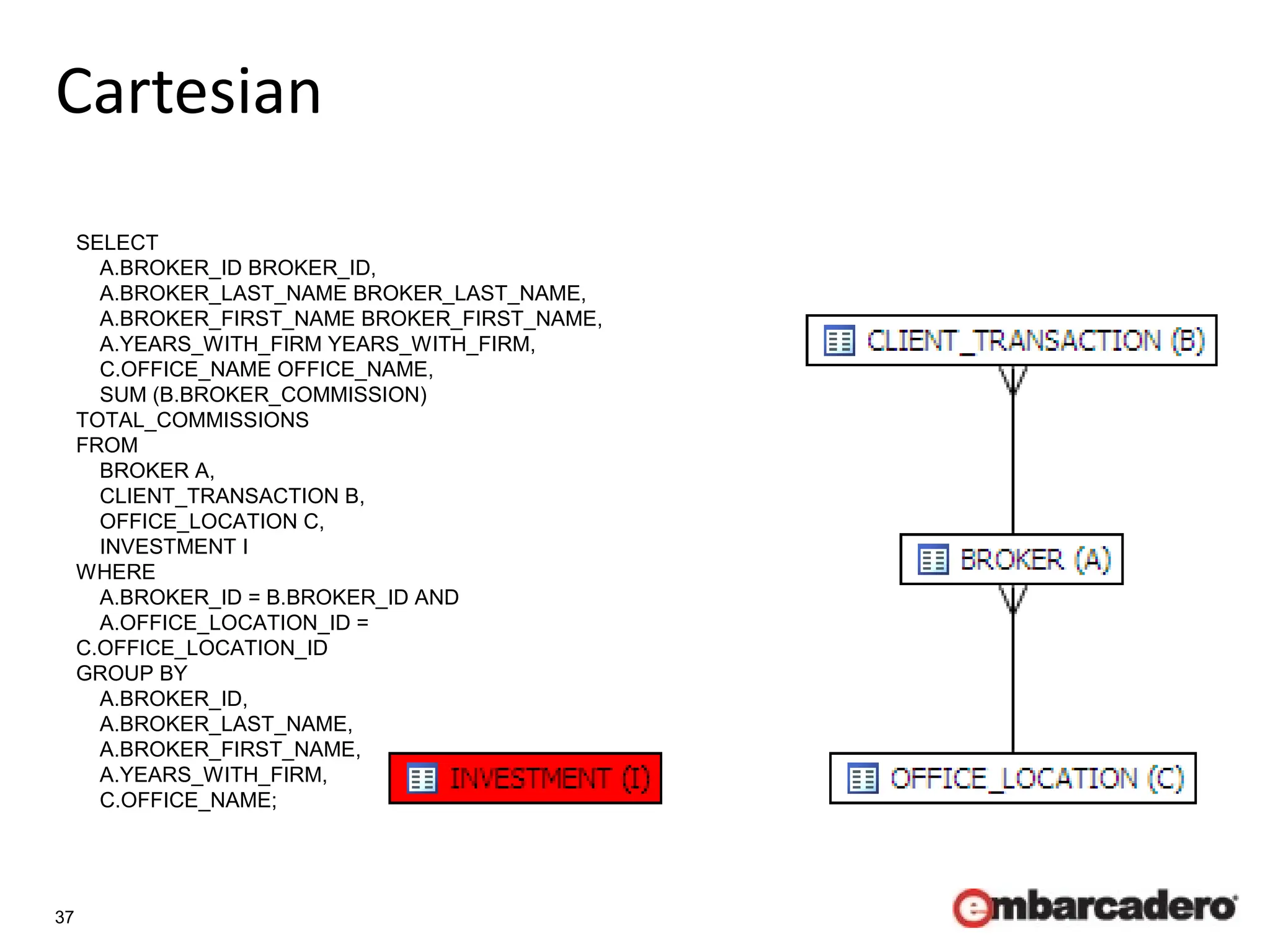
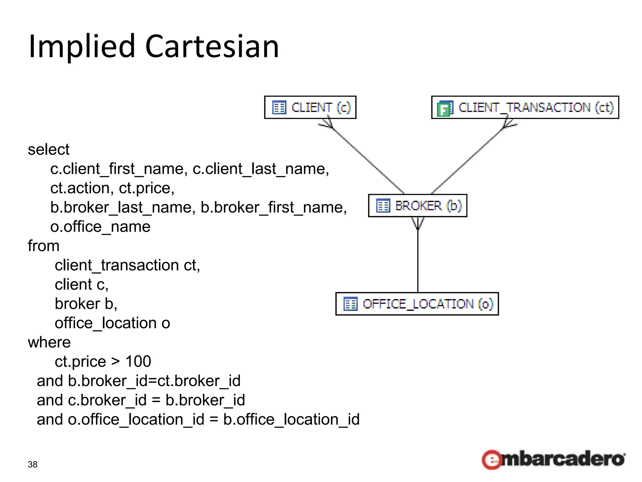
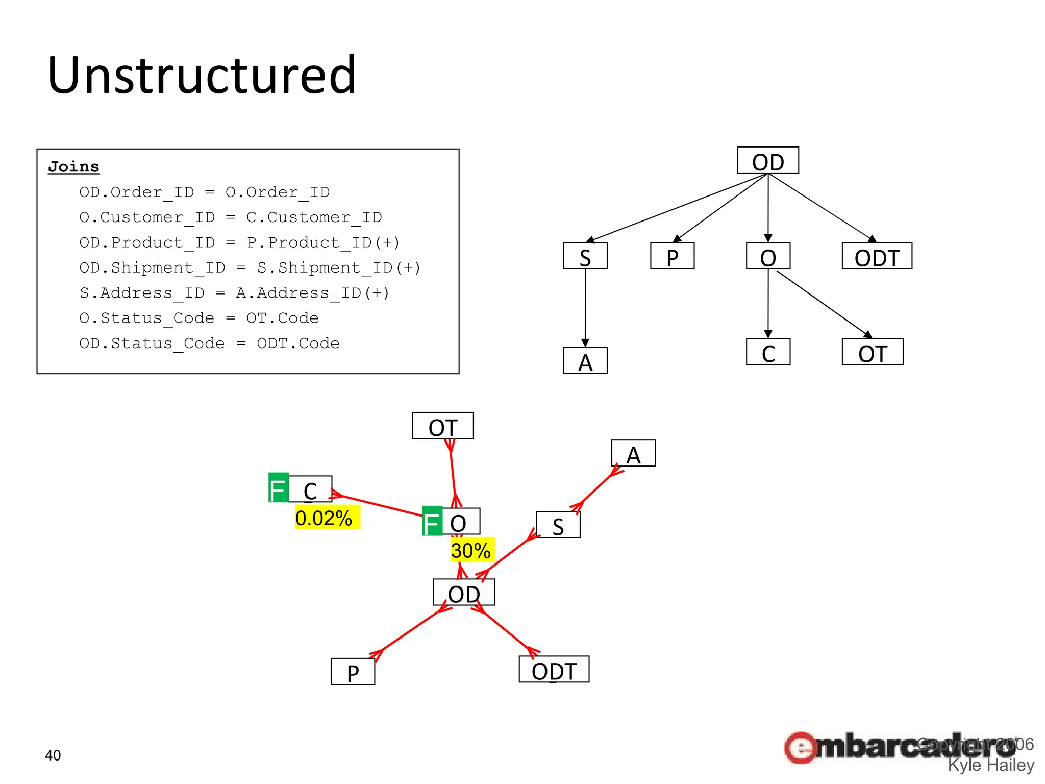
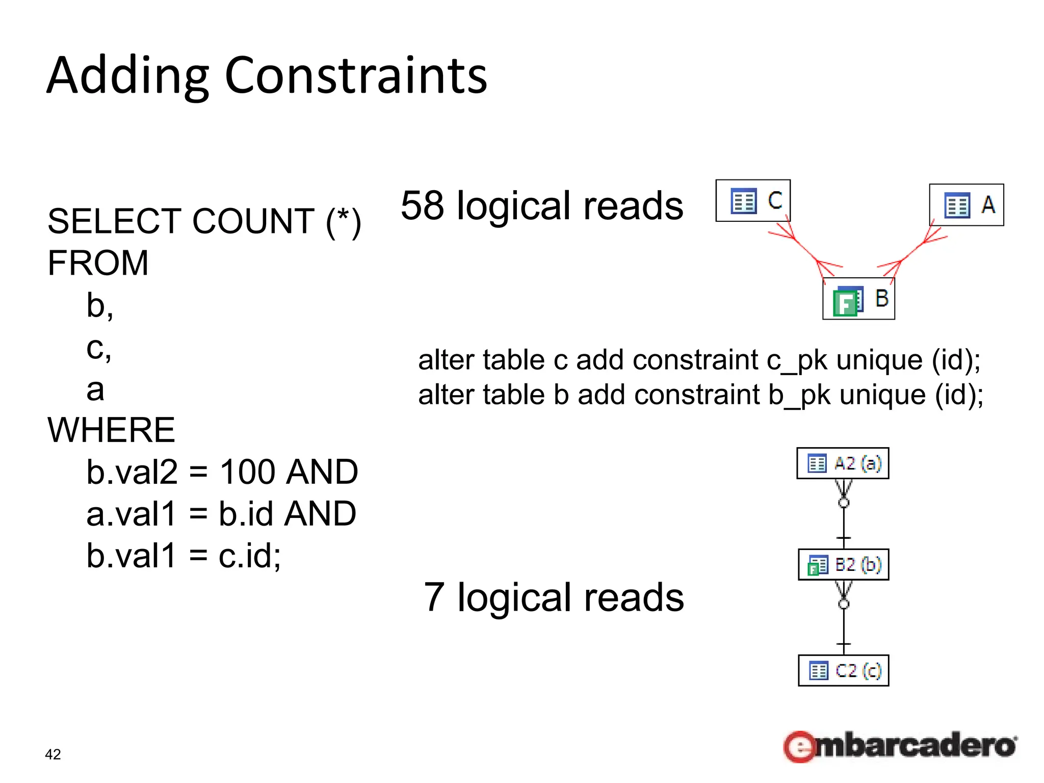
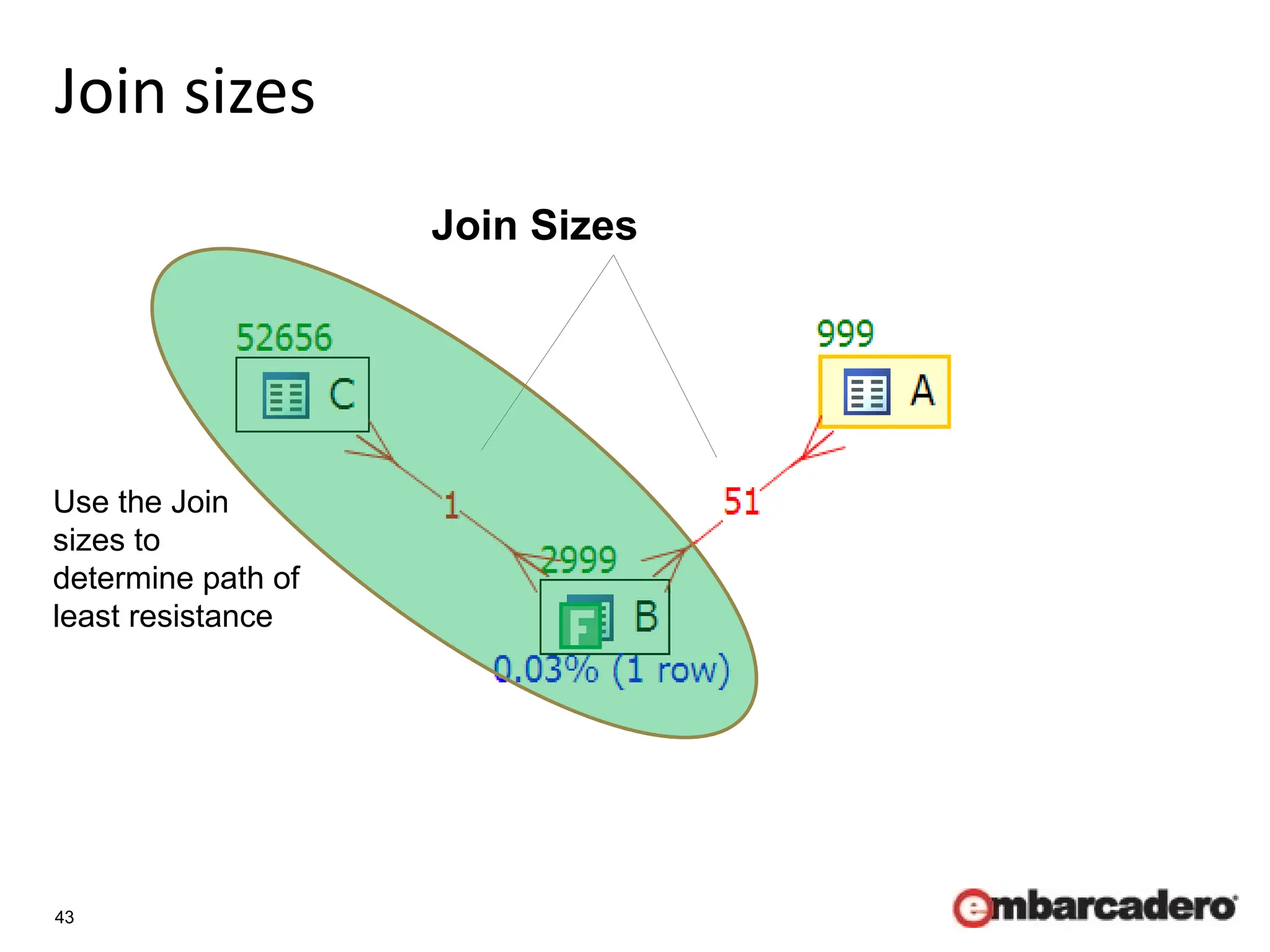
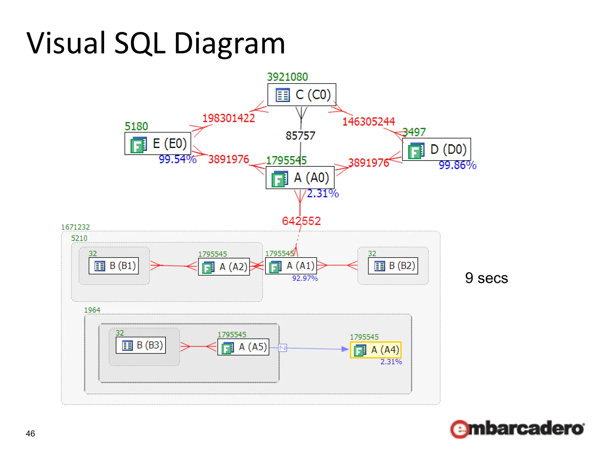
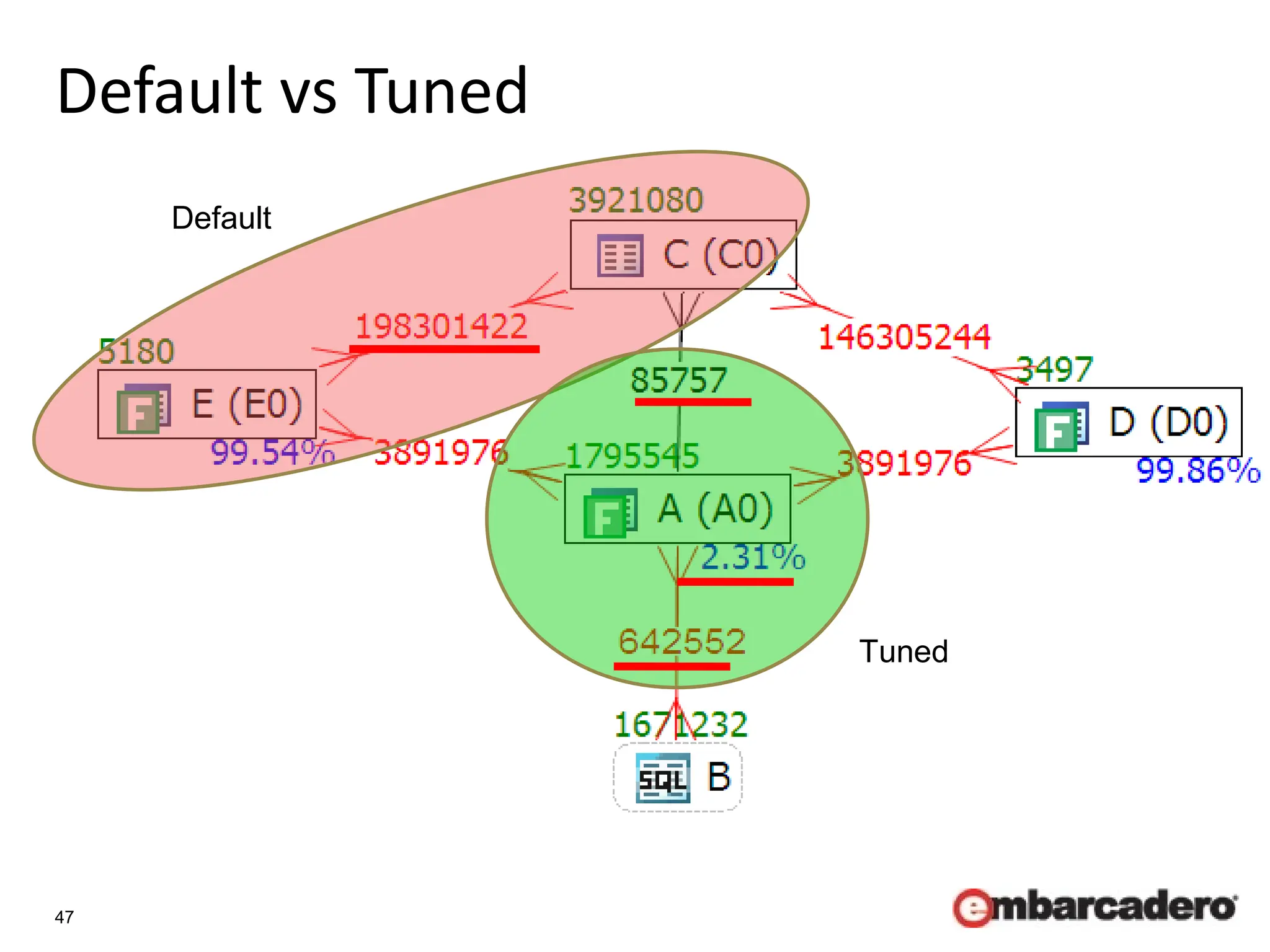
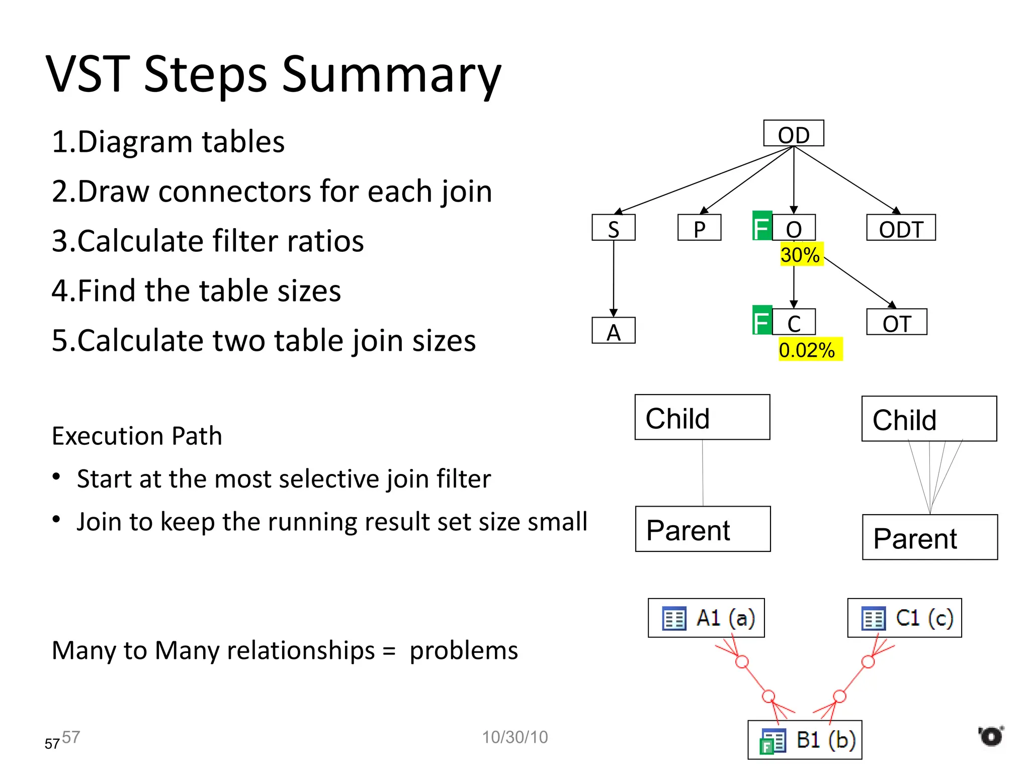
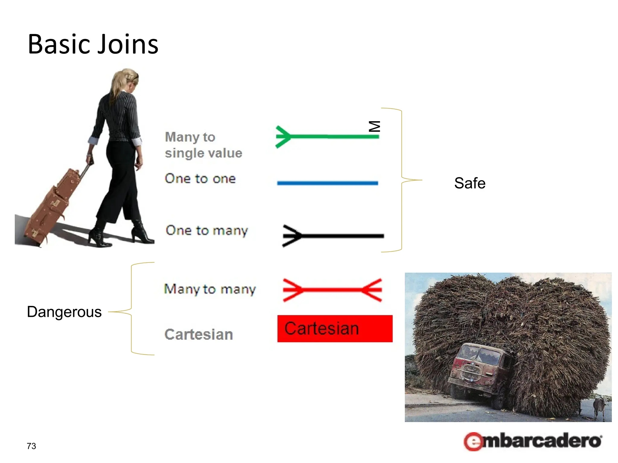
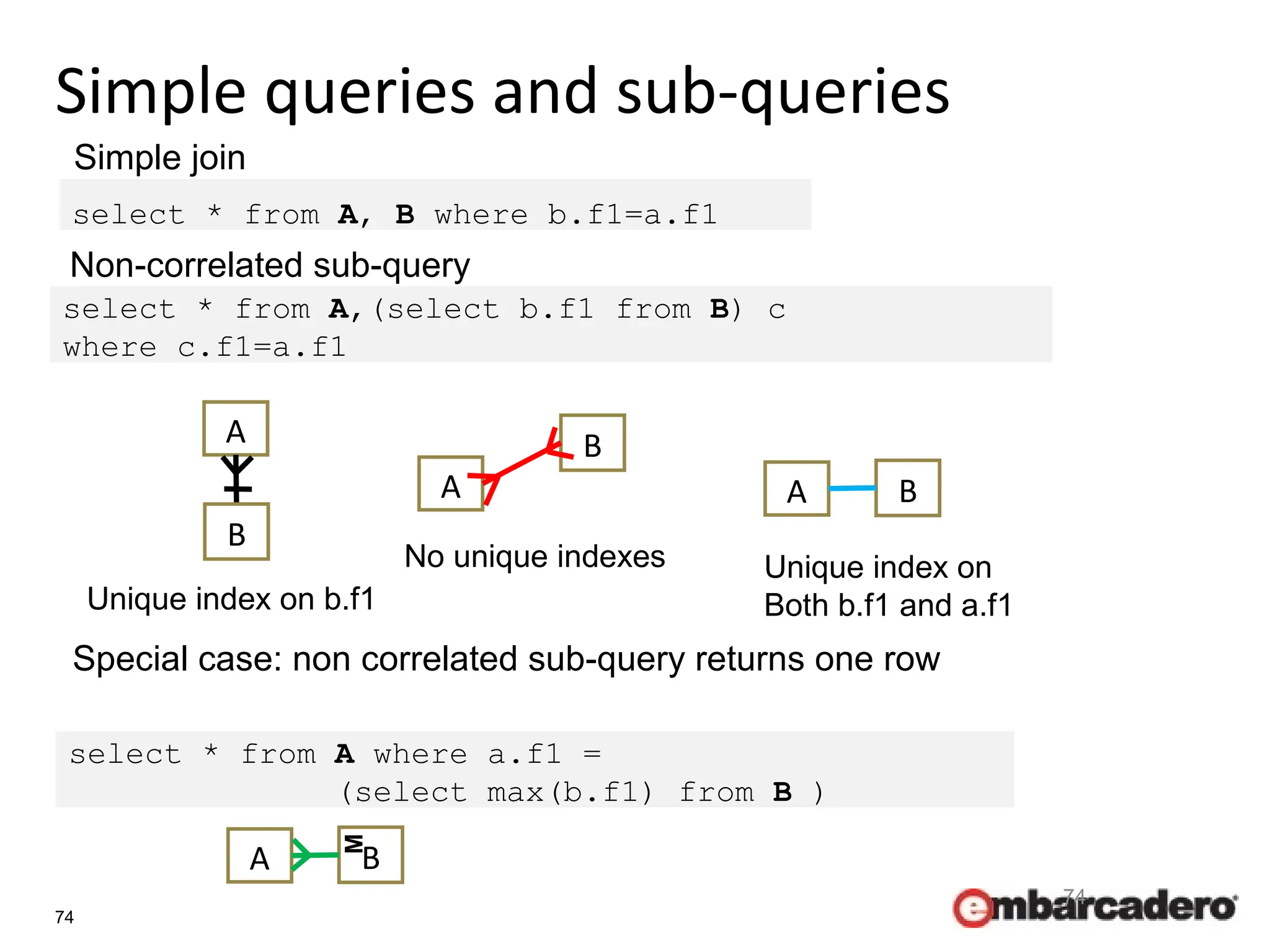
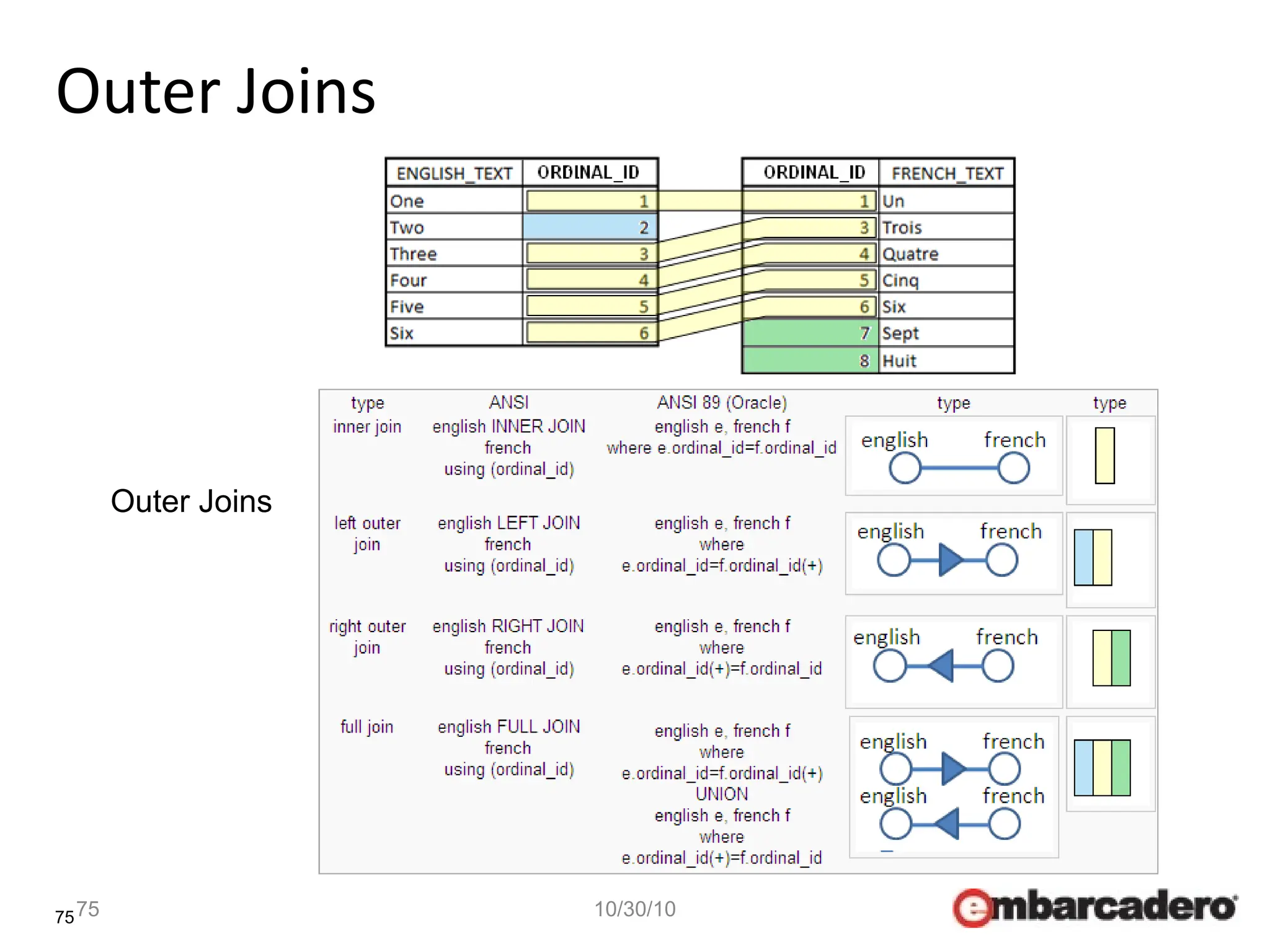
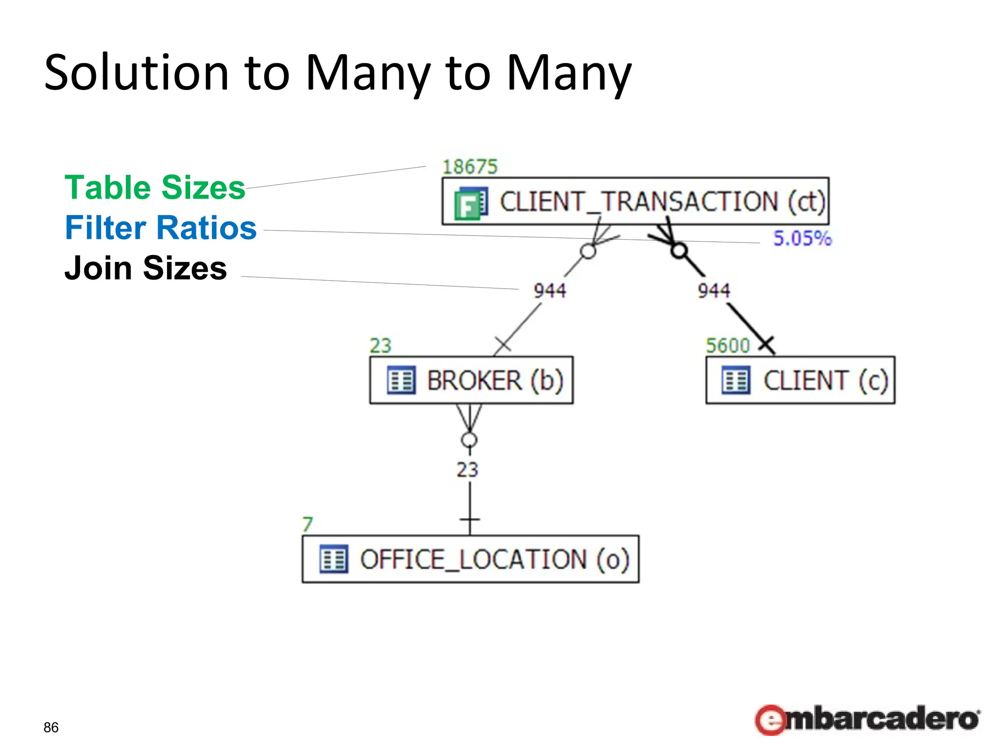
2. Key steps in visual SQL tuning are laid out, including drawing tables as nodes, joins as connection lines, and filters as markings on tables. This helps identify optimization opportunities like missing indexes or stale statistics.
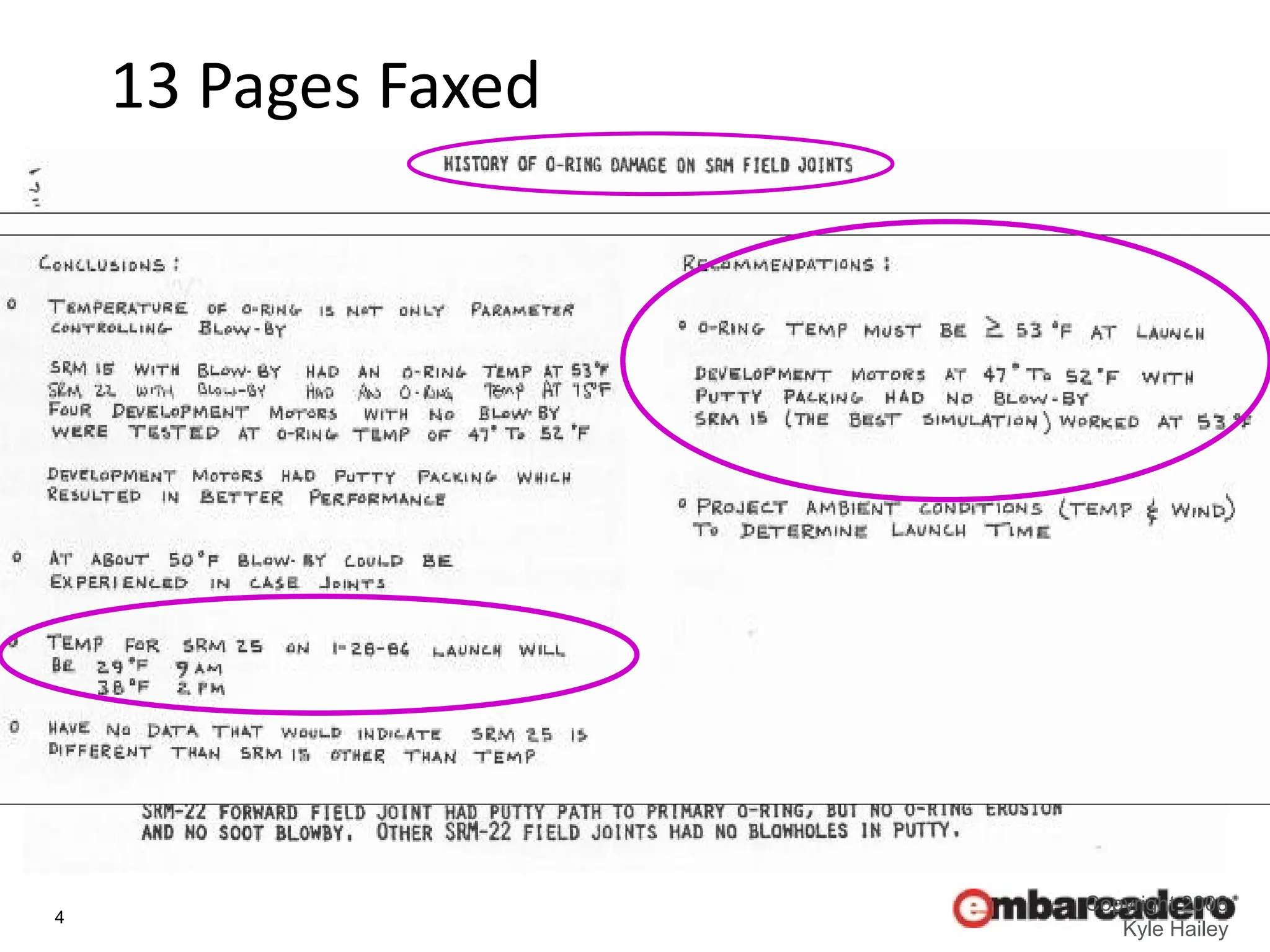
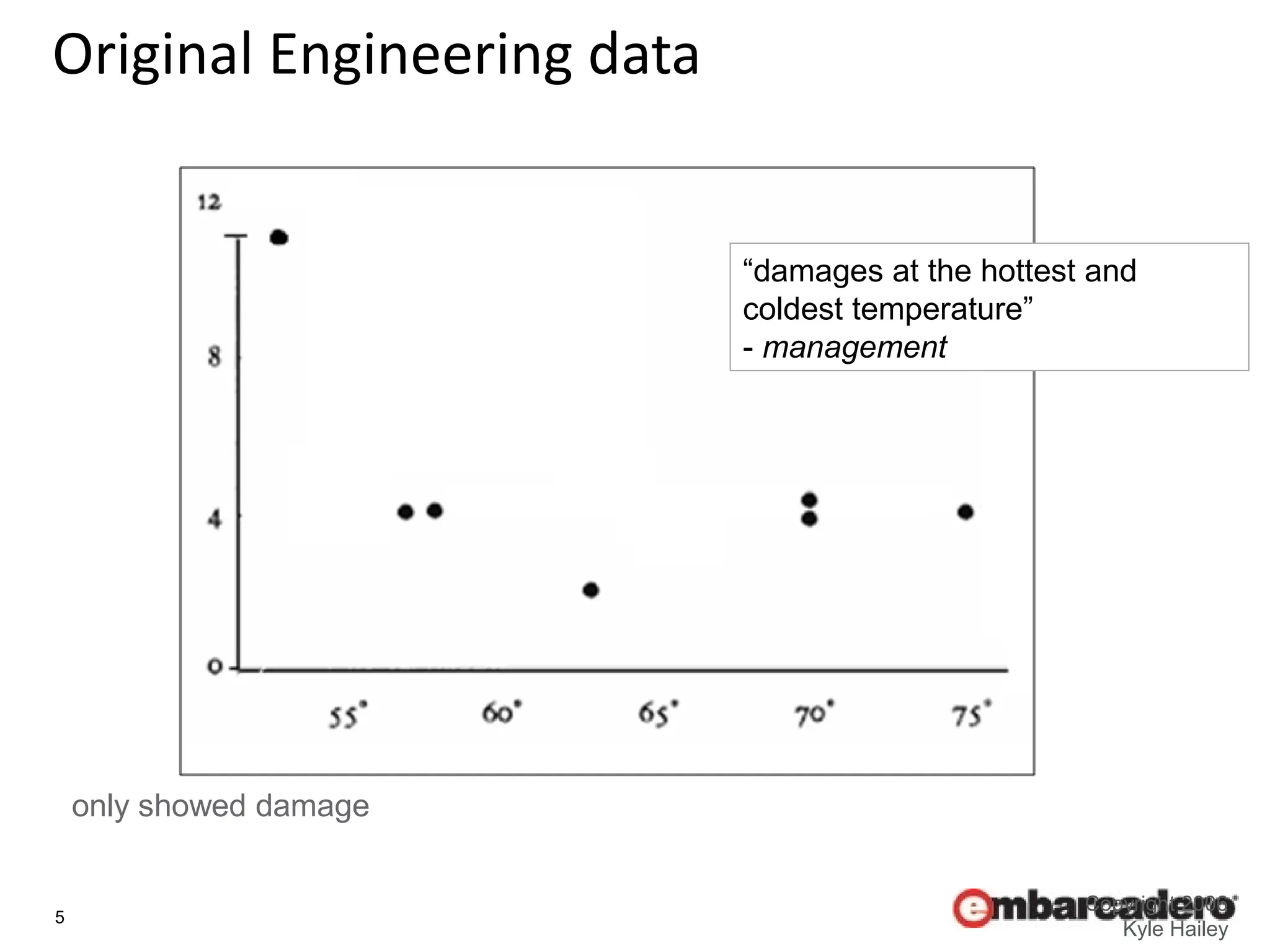
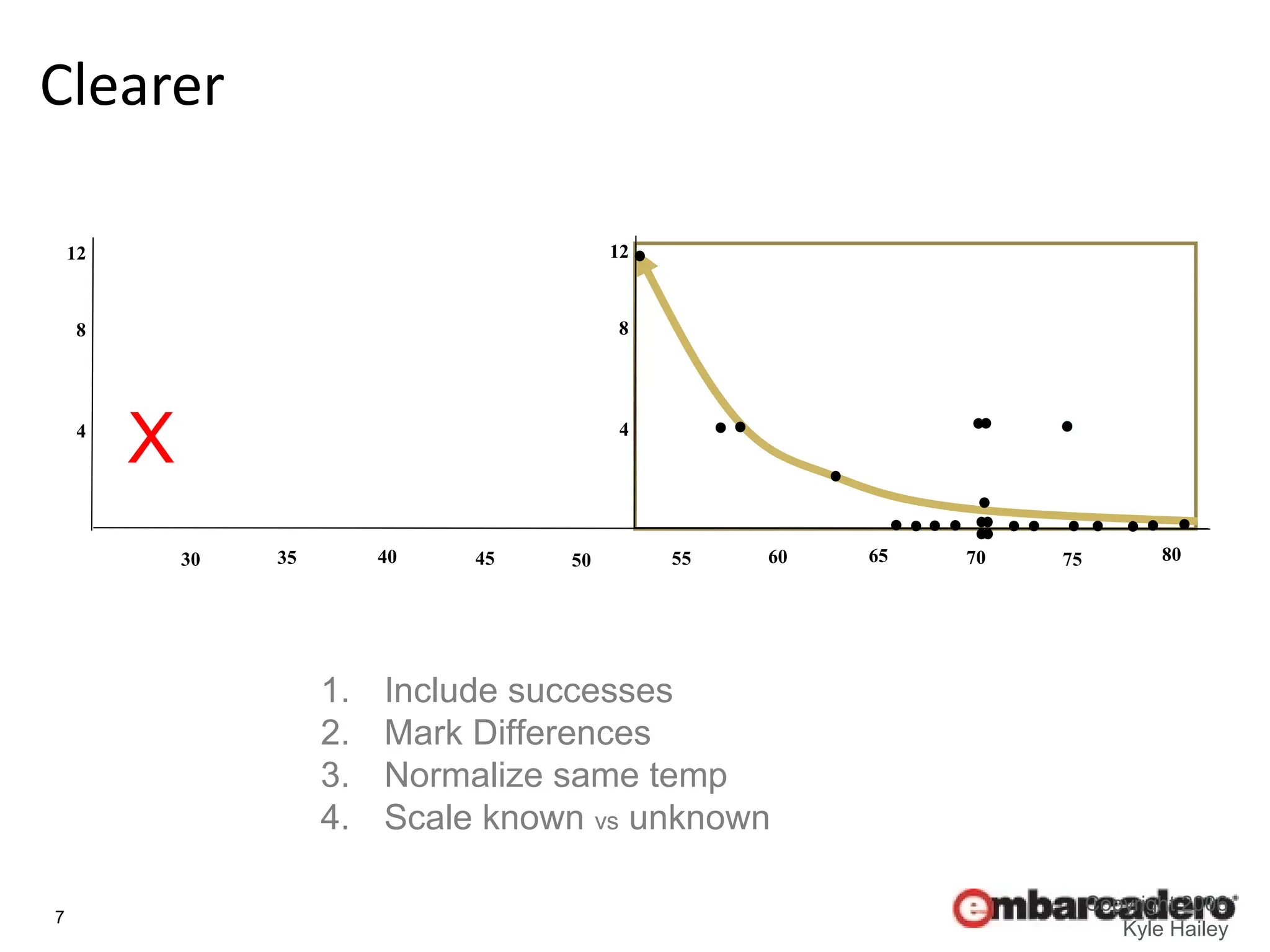
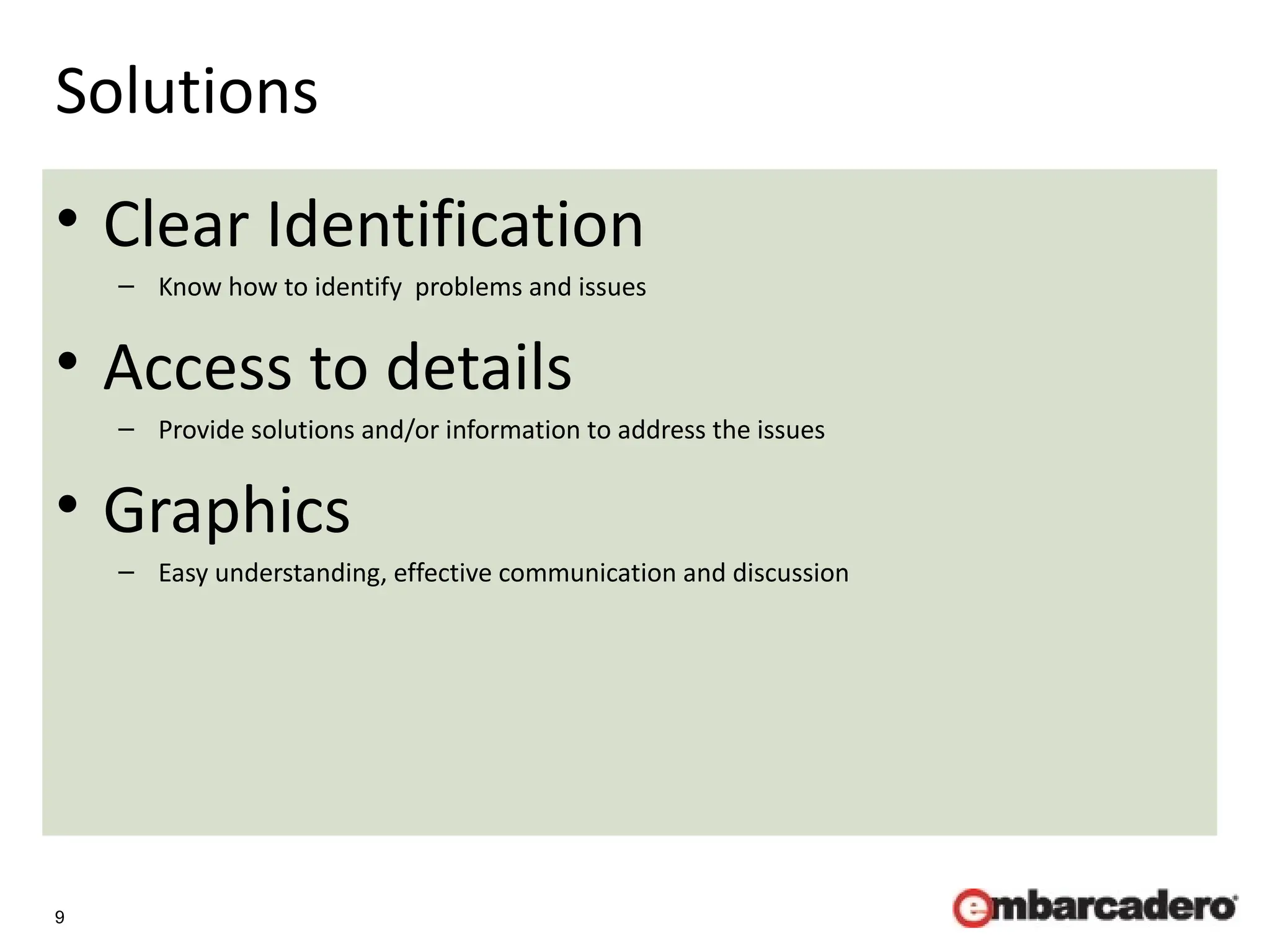
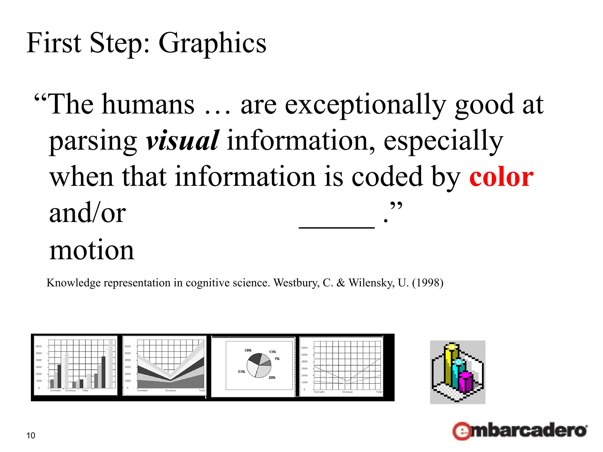
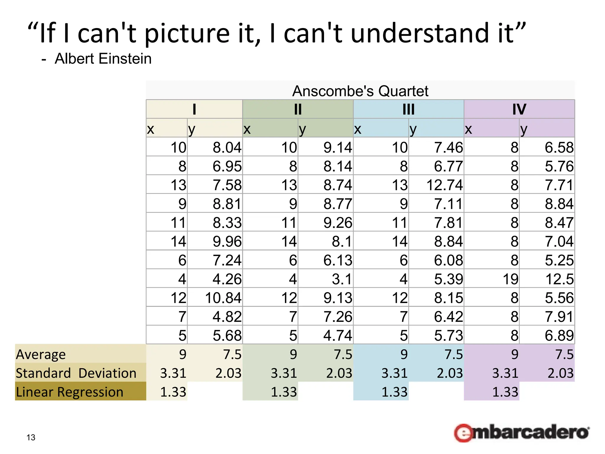
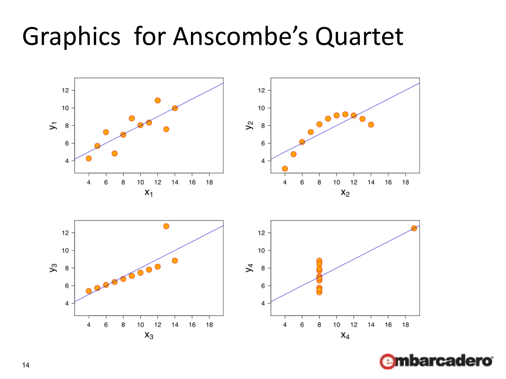
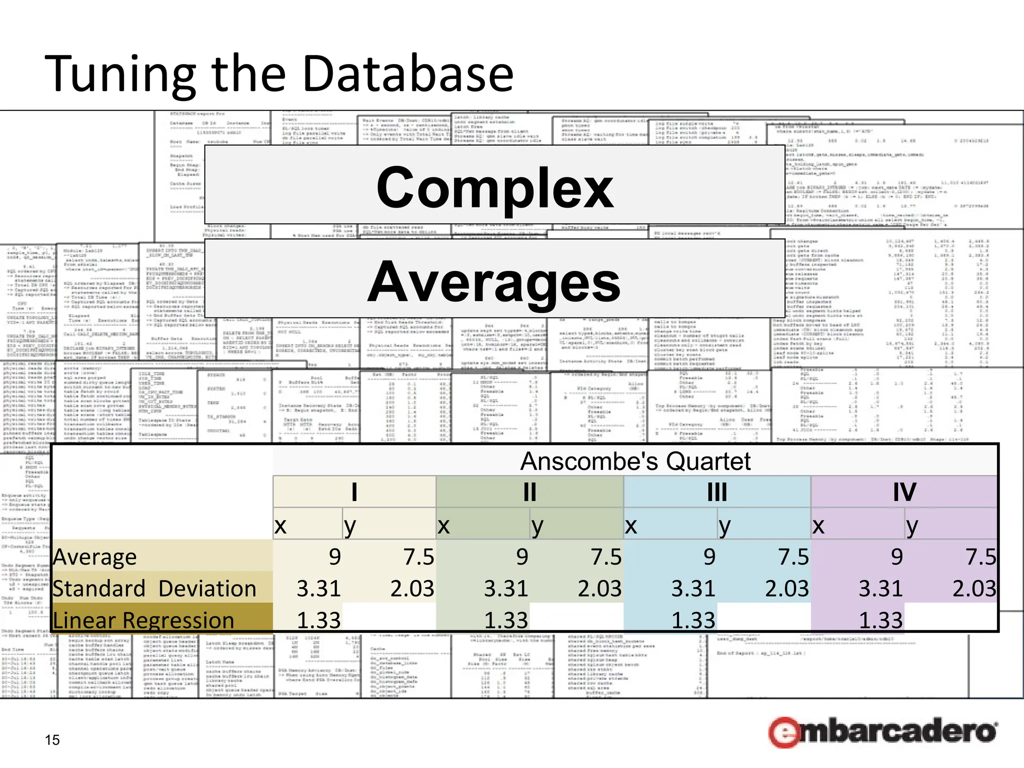
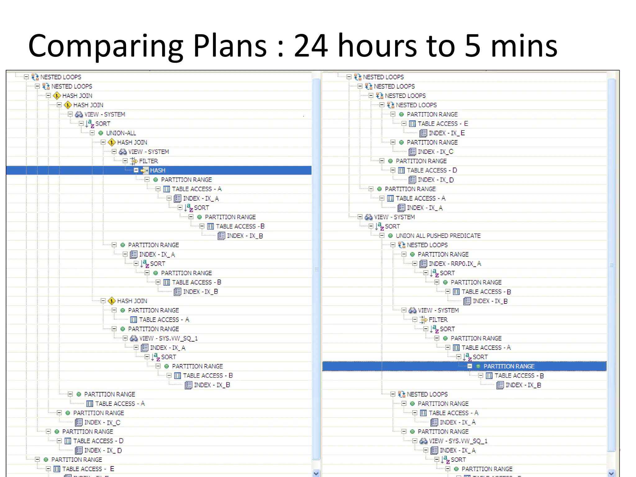
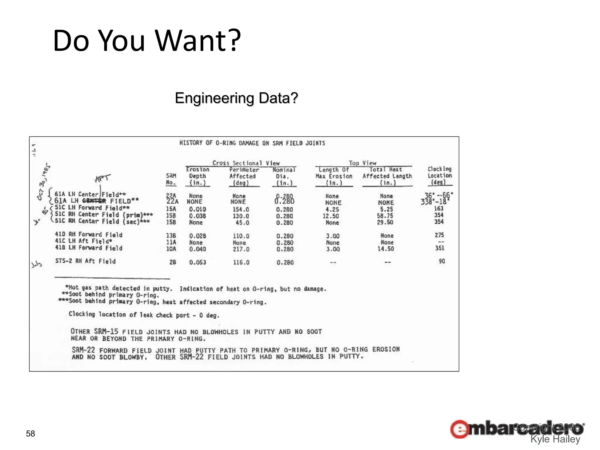
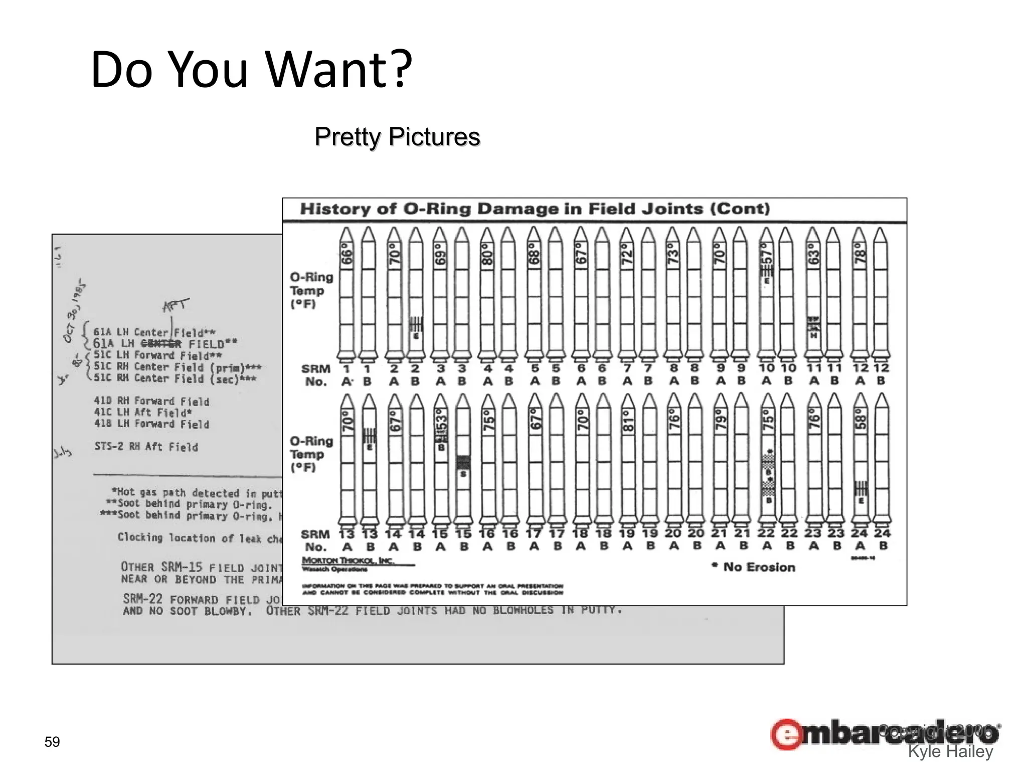
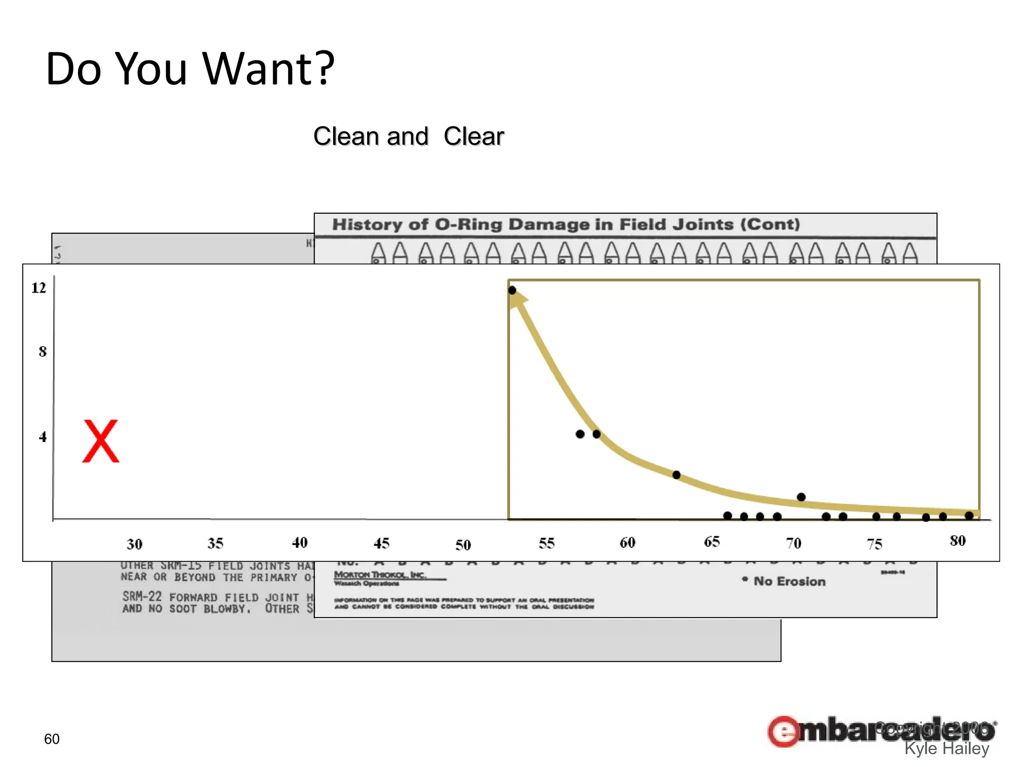
3. The document emphasizes that a lack of clarity in visualizing complex data and queries can have devastating consequences, while graphics enable easy understanding and effective problem-solving.