The document summarizes the amortized analysis of several data structures and algorithms:
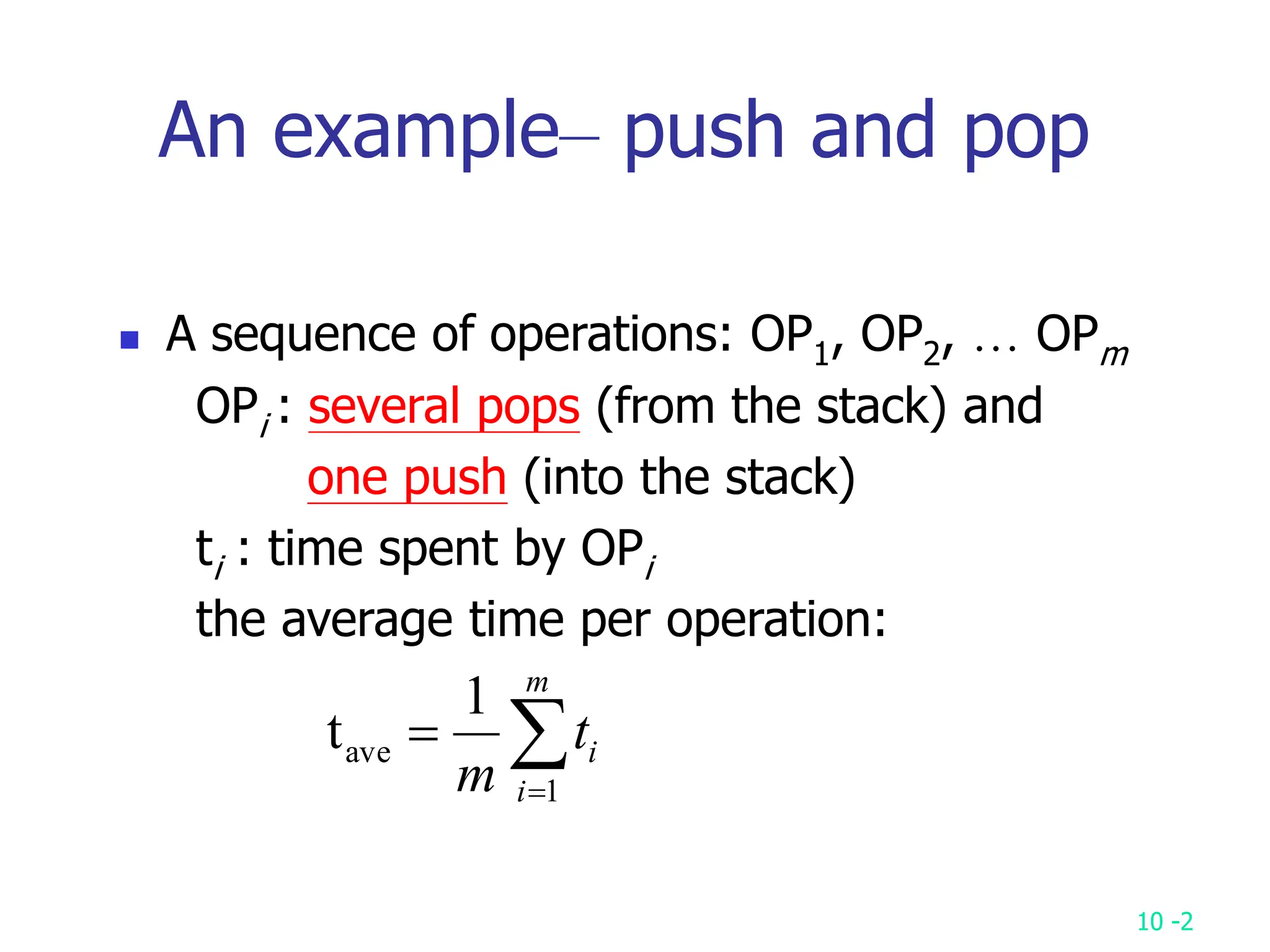
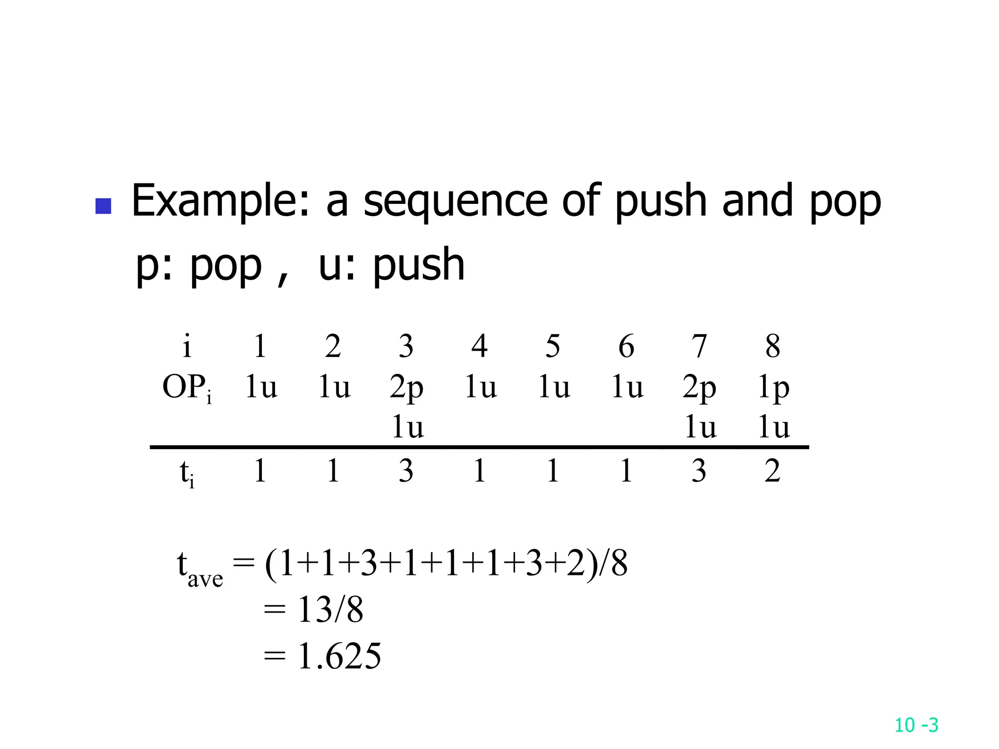
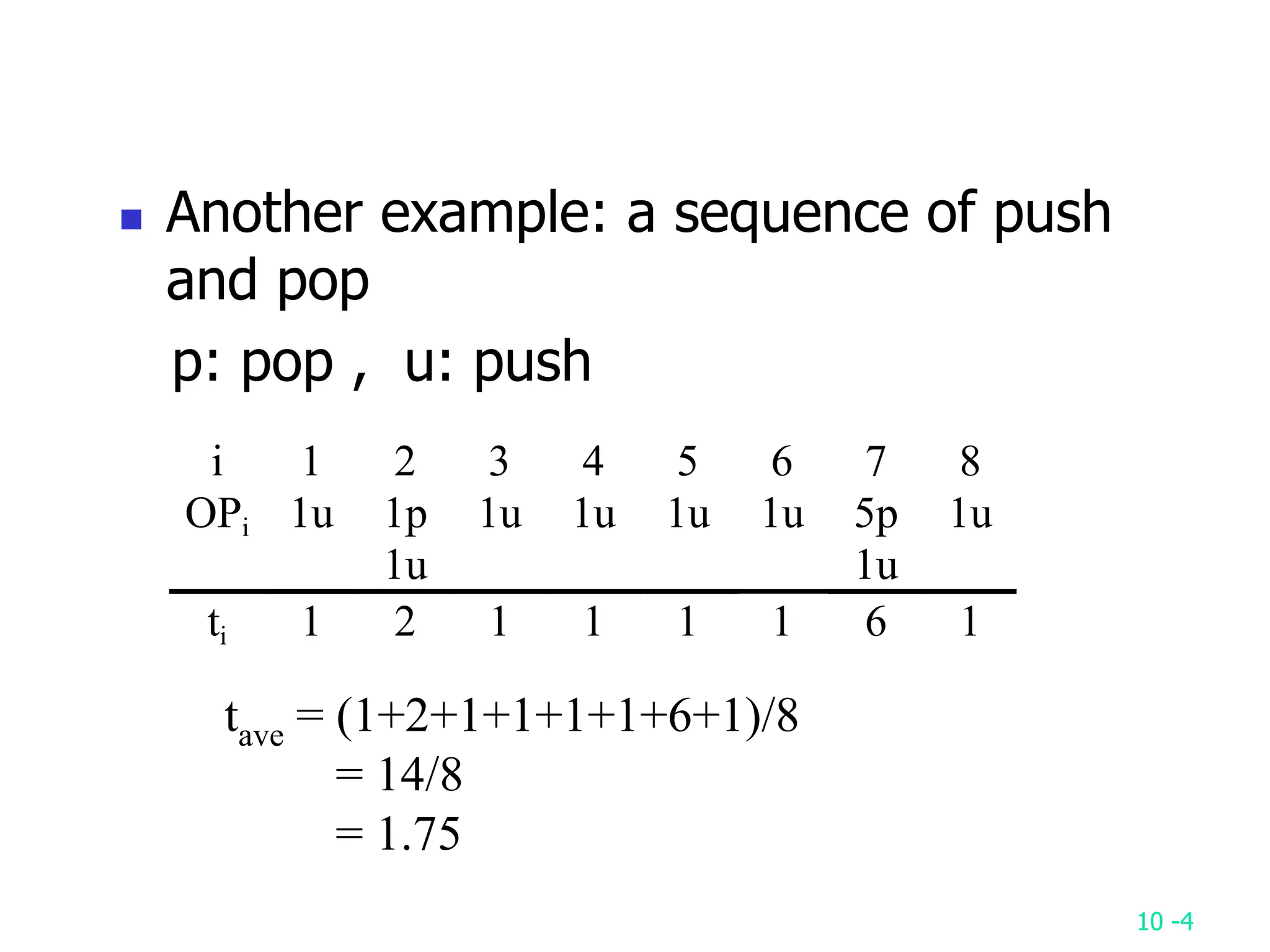
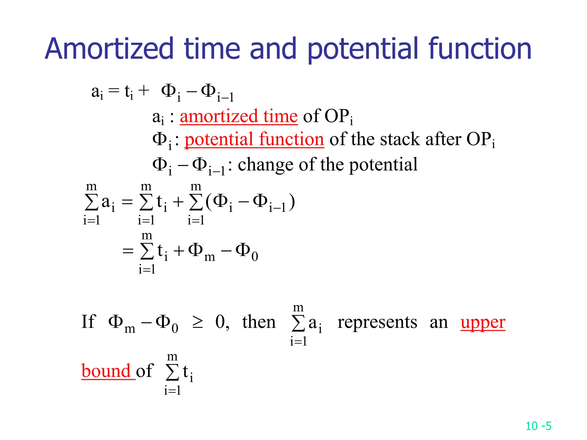
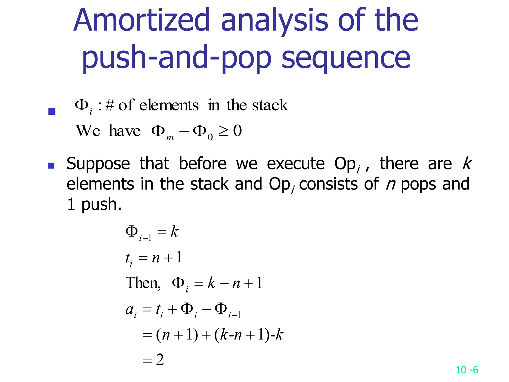
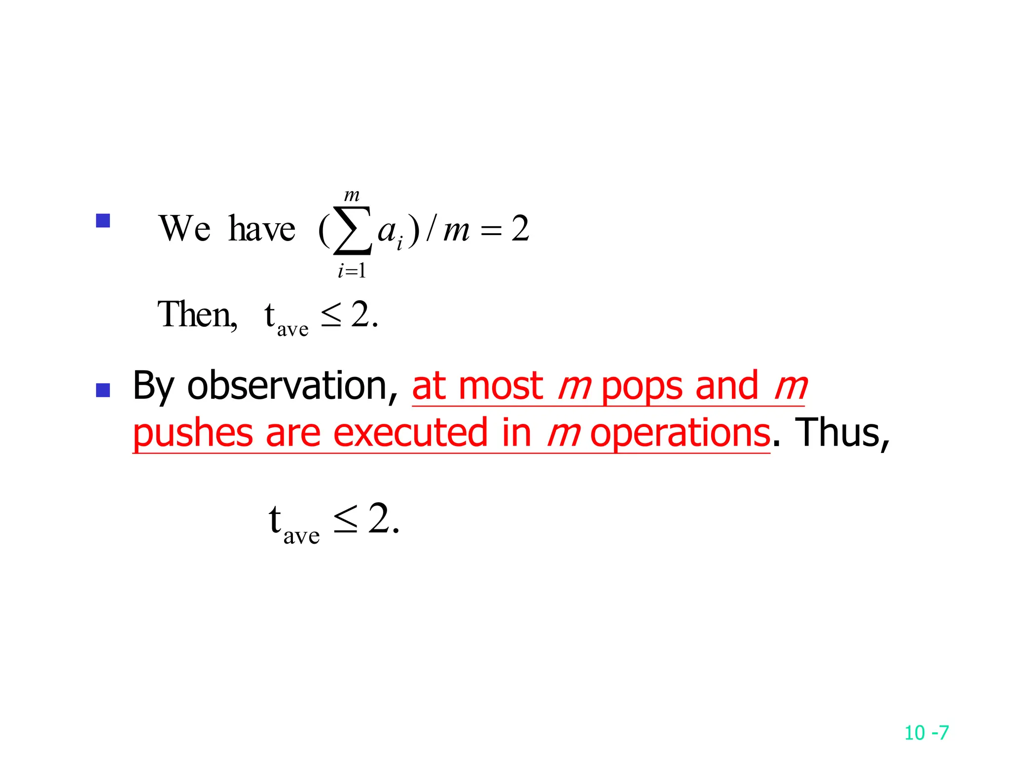
1. It introduces the concept of amortized analysis and uses examples of push and pop operations on a stack to show how to calculate the amortized time per operation.
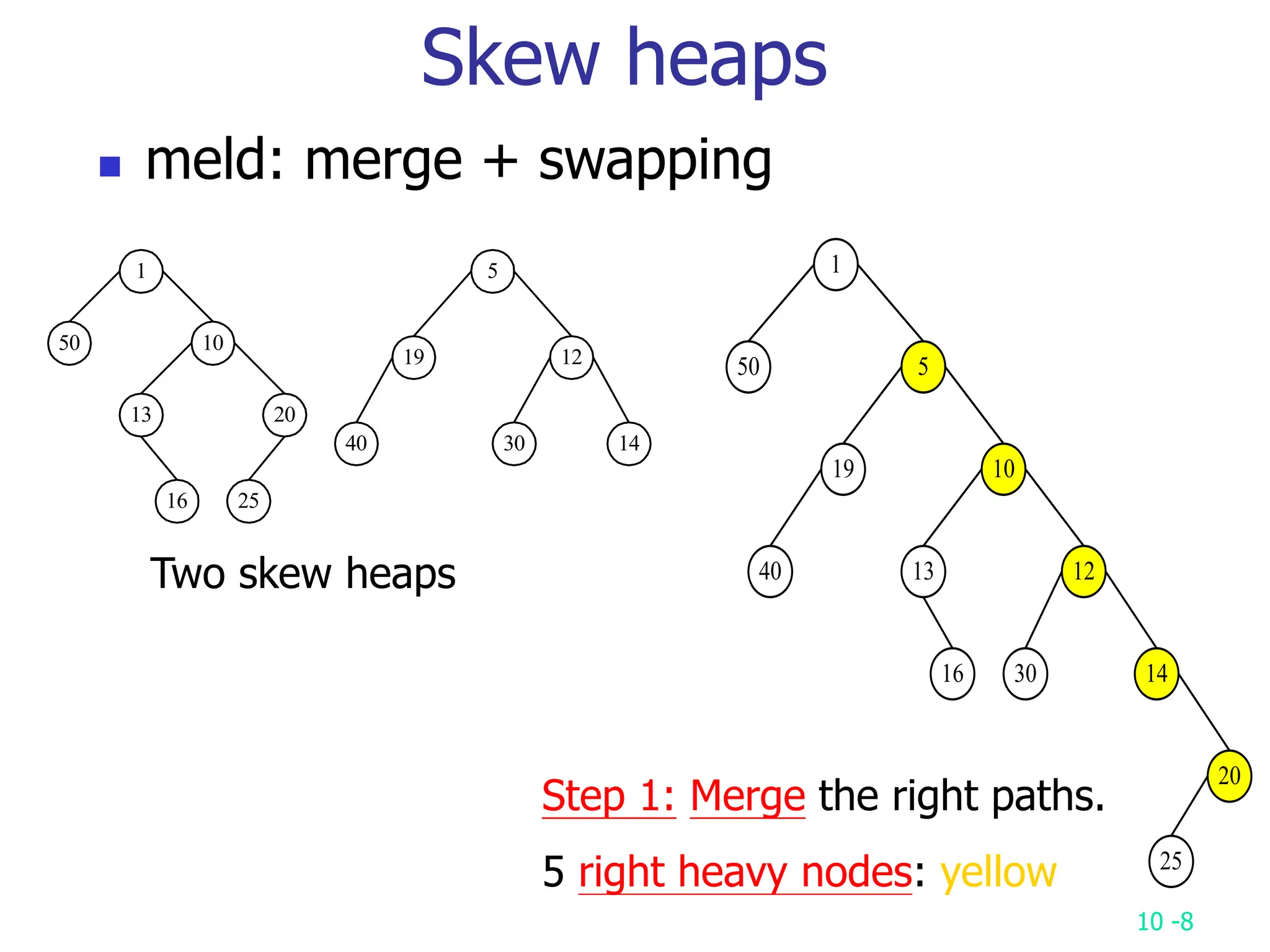
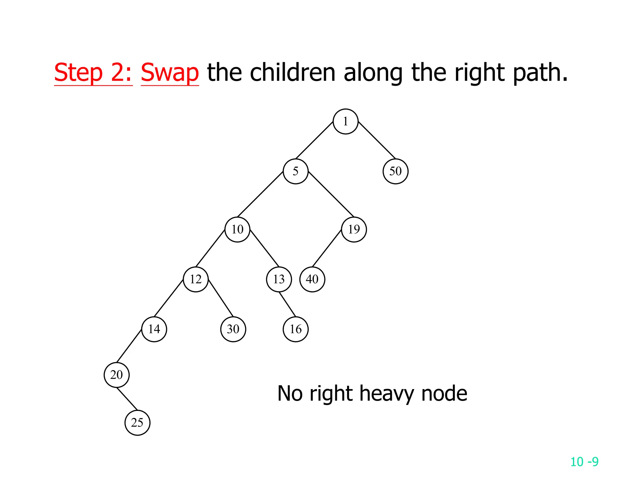
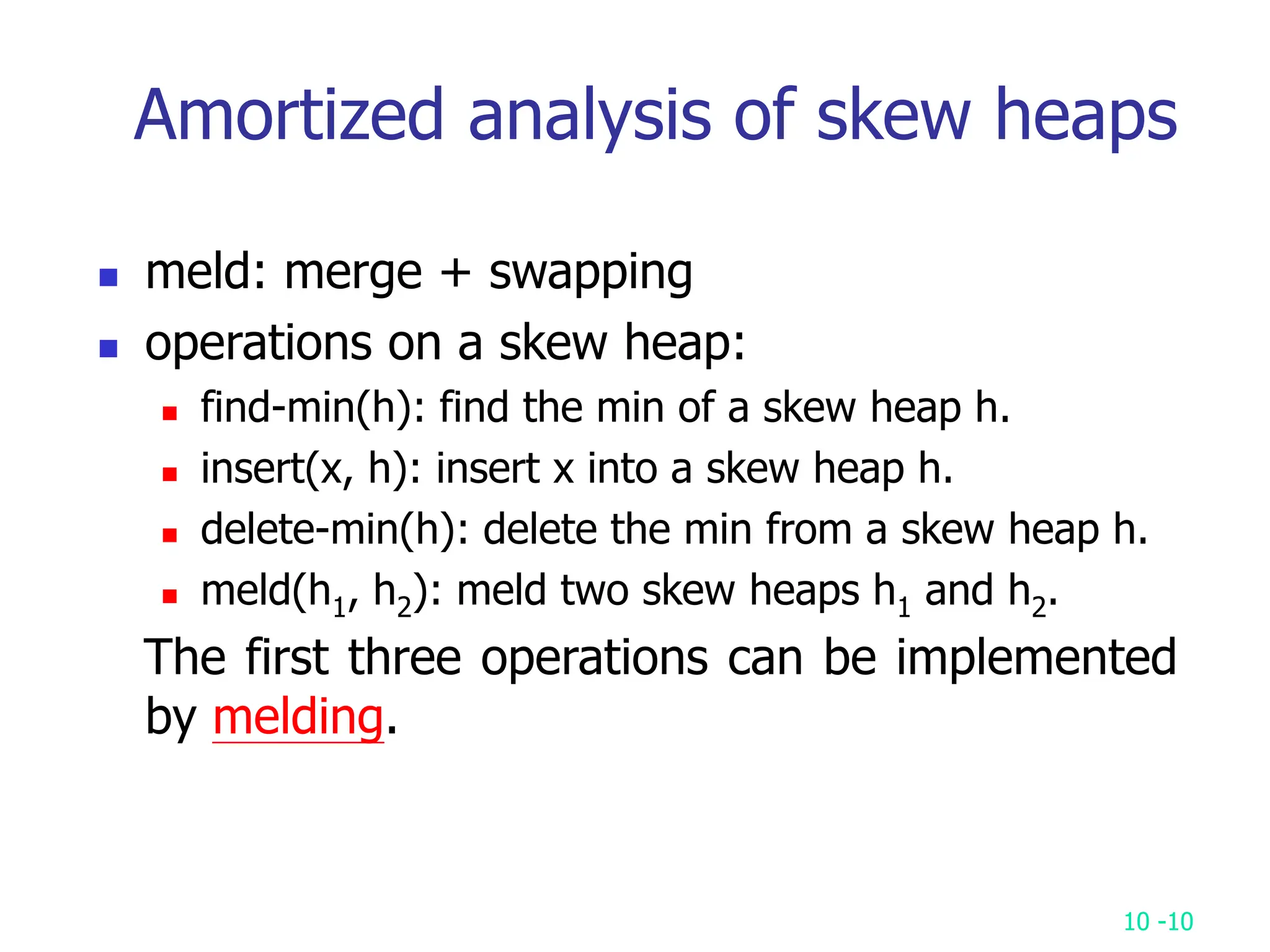
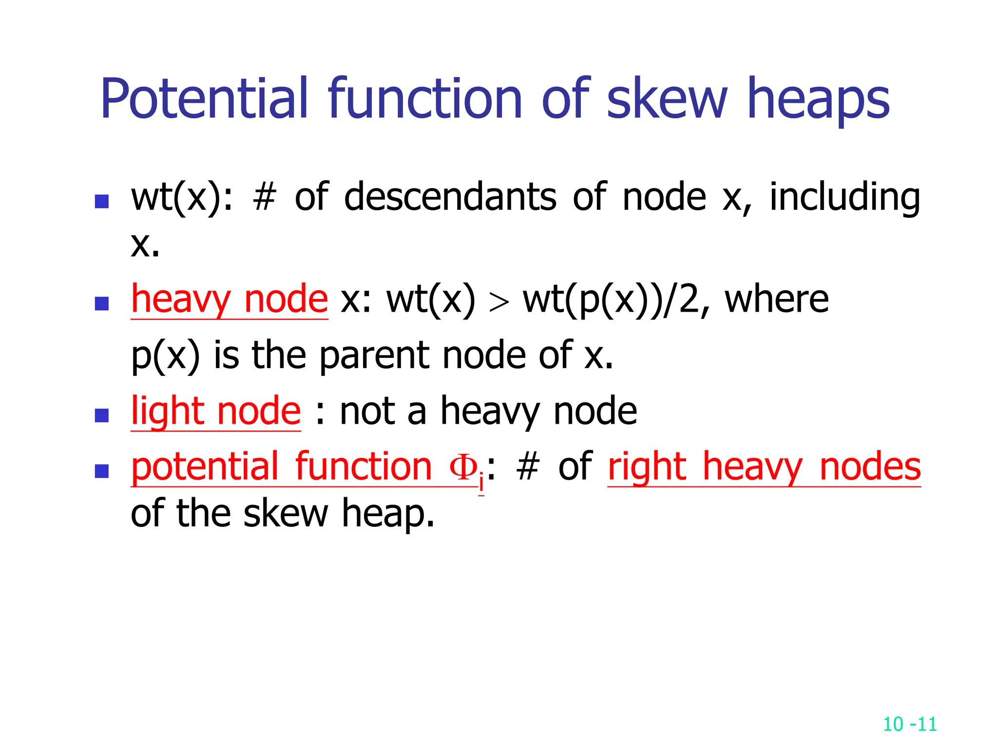
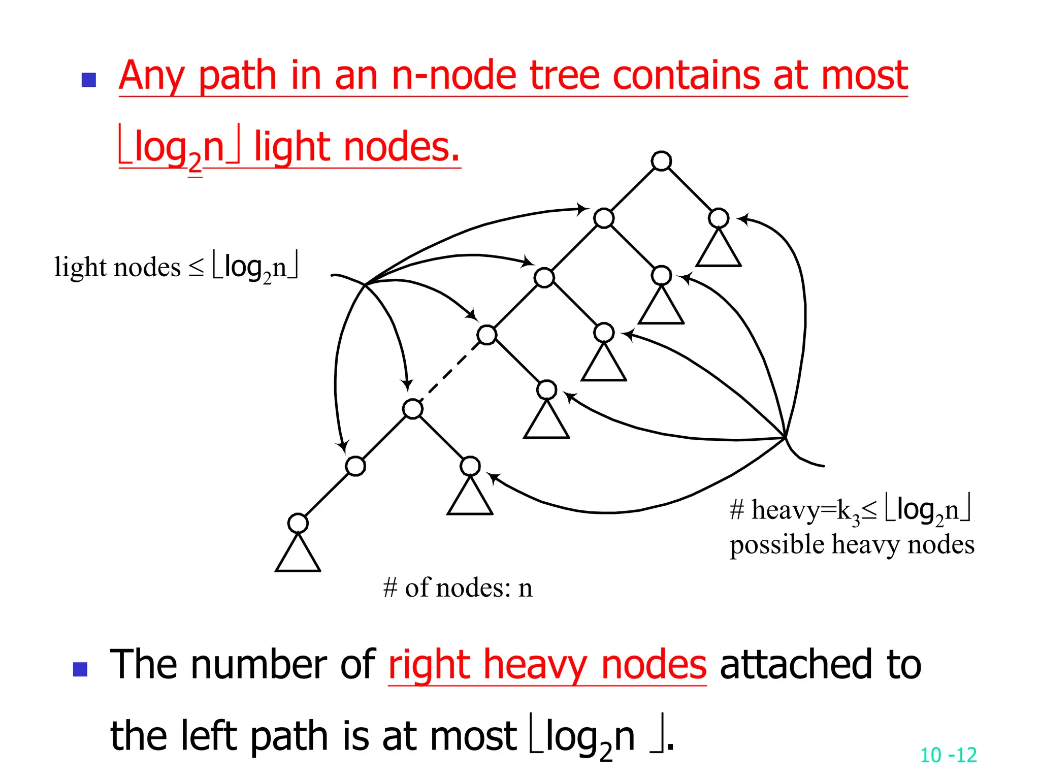
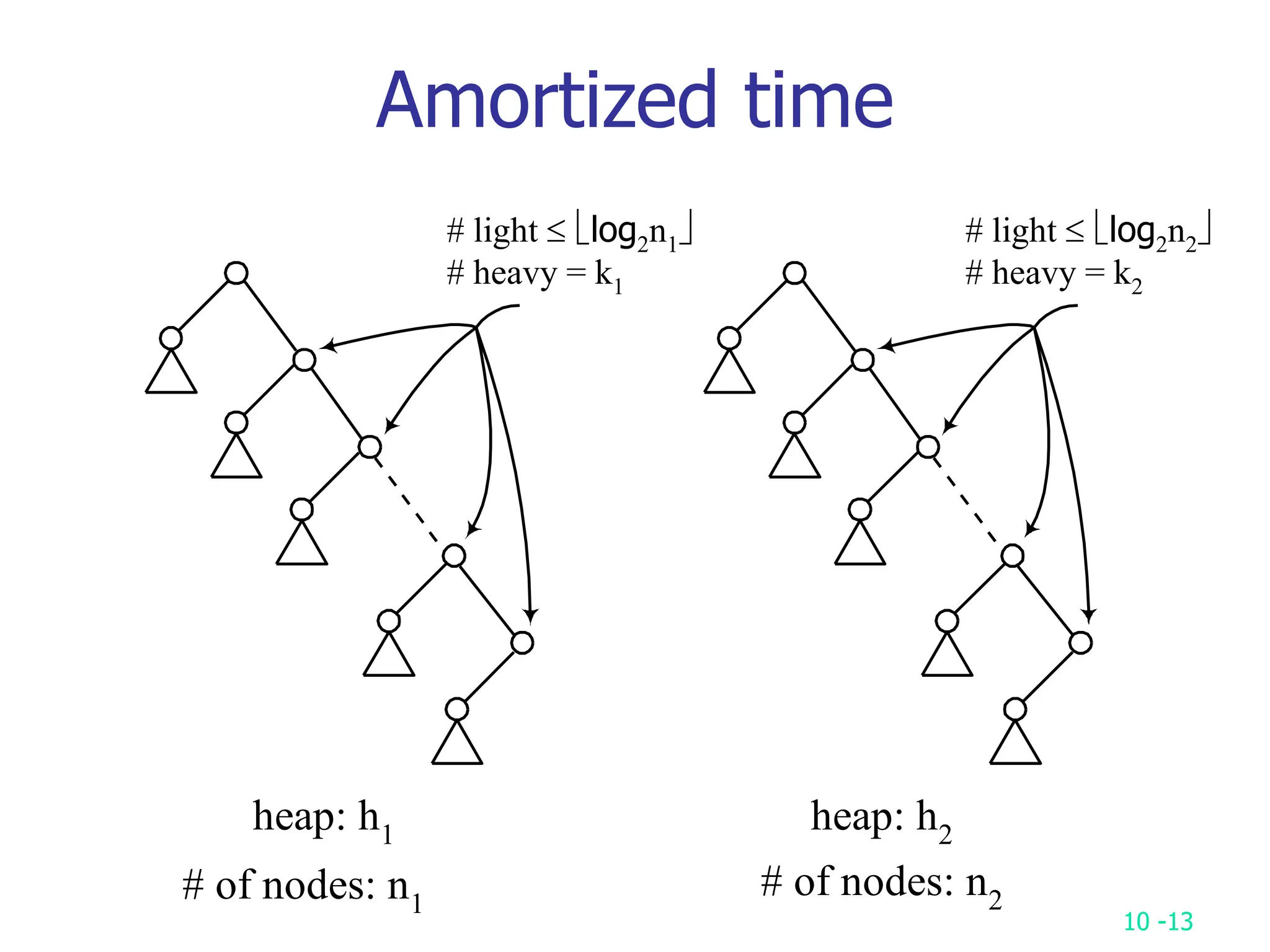
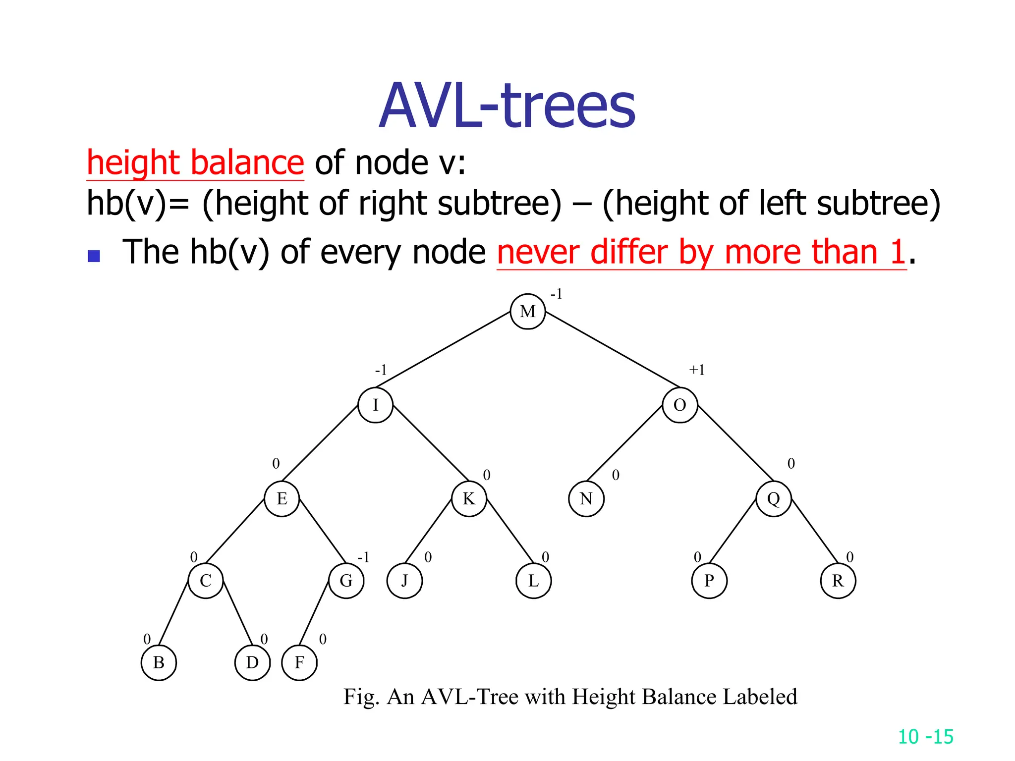
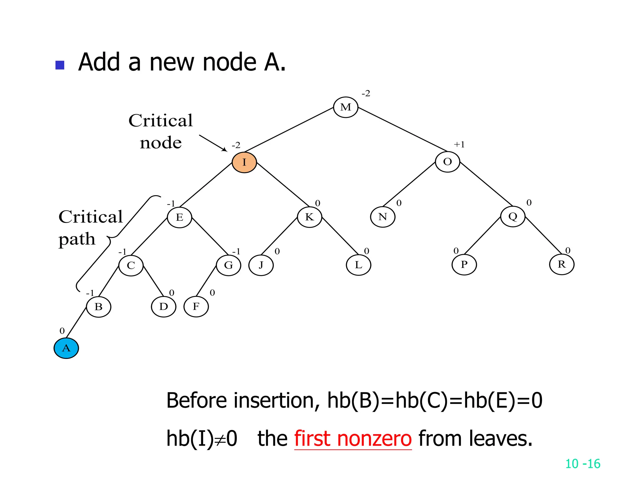
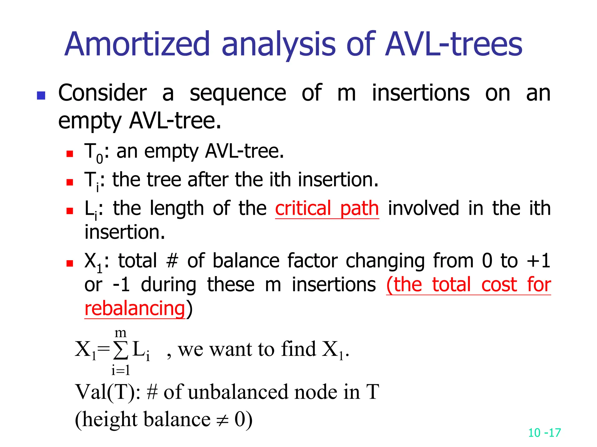
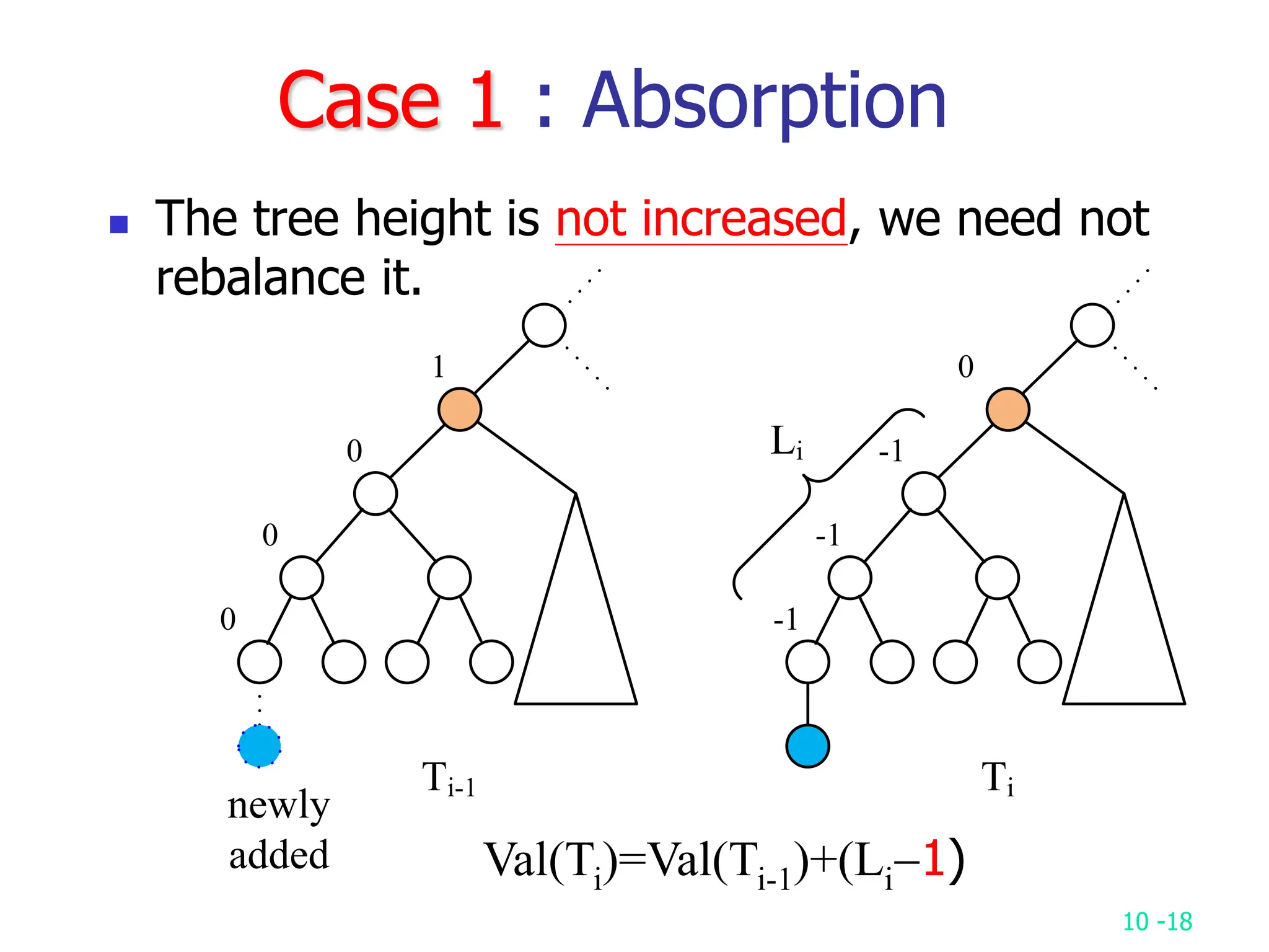
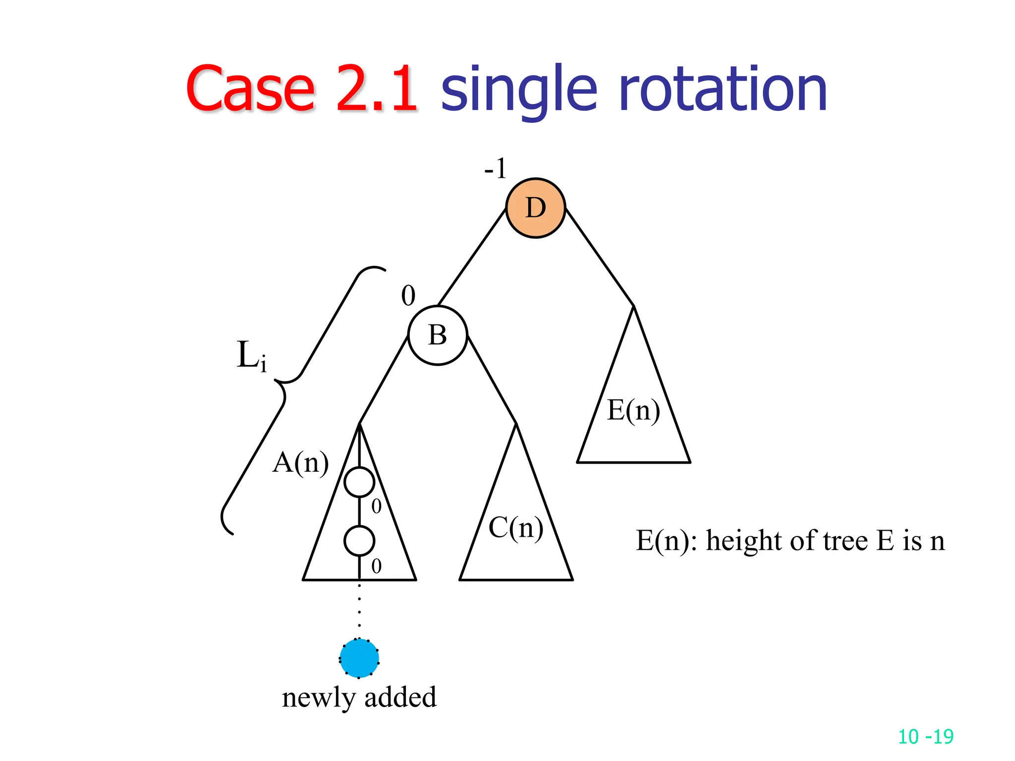
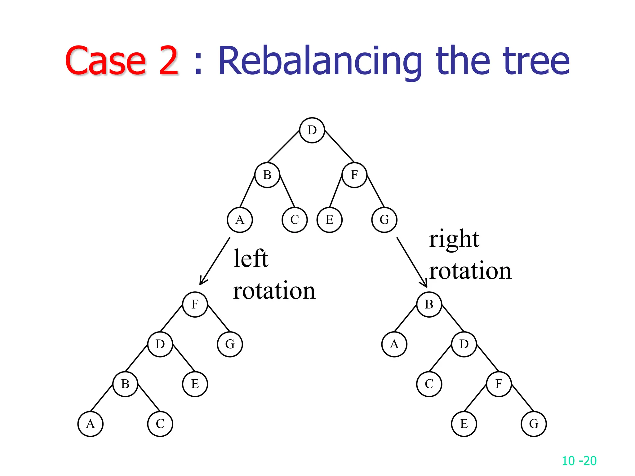
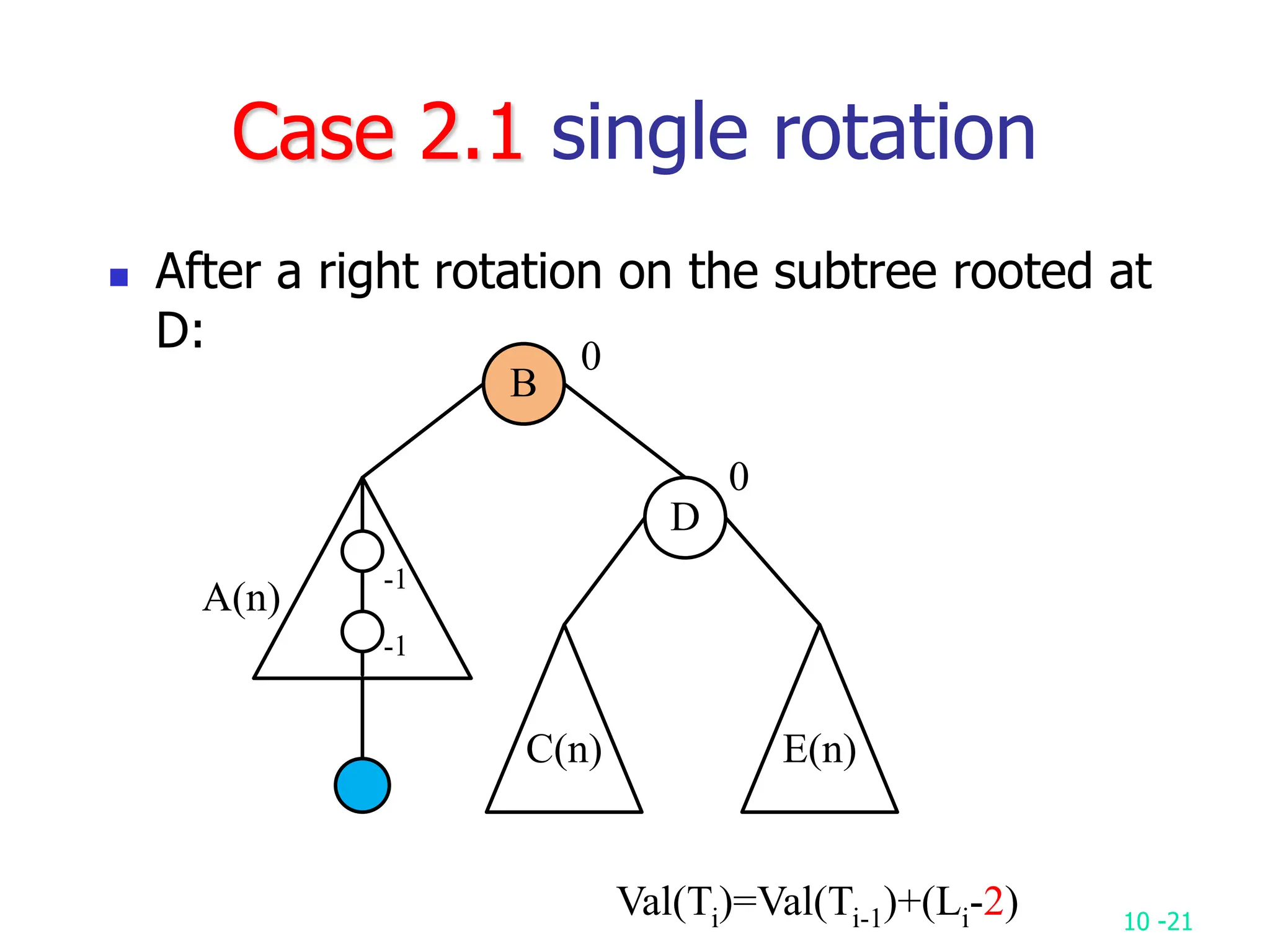
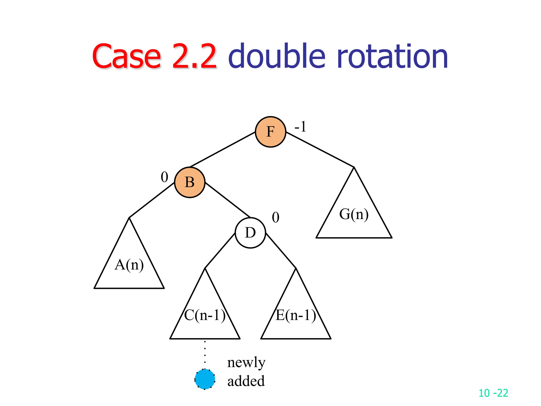
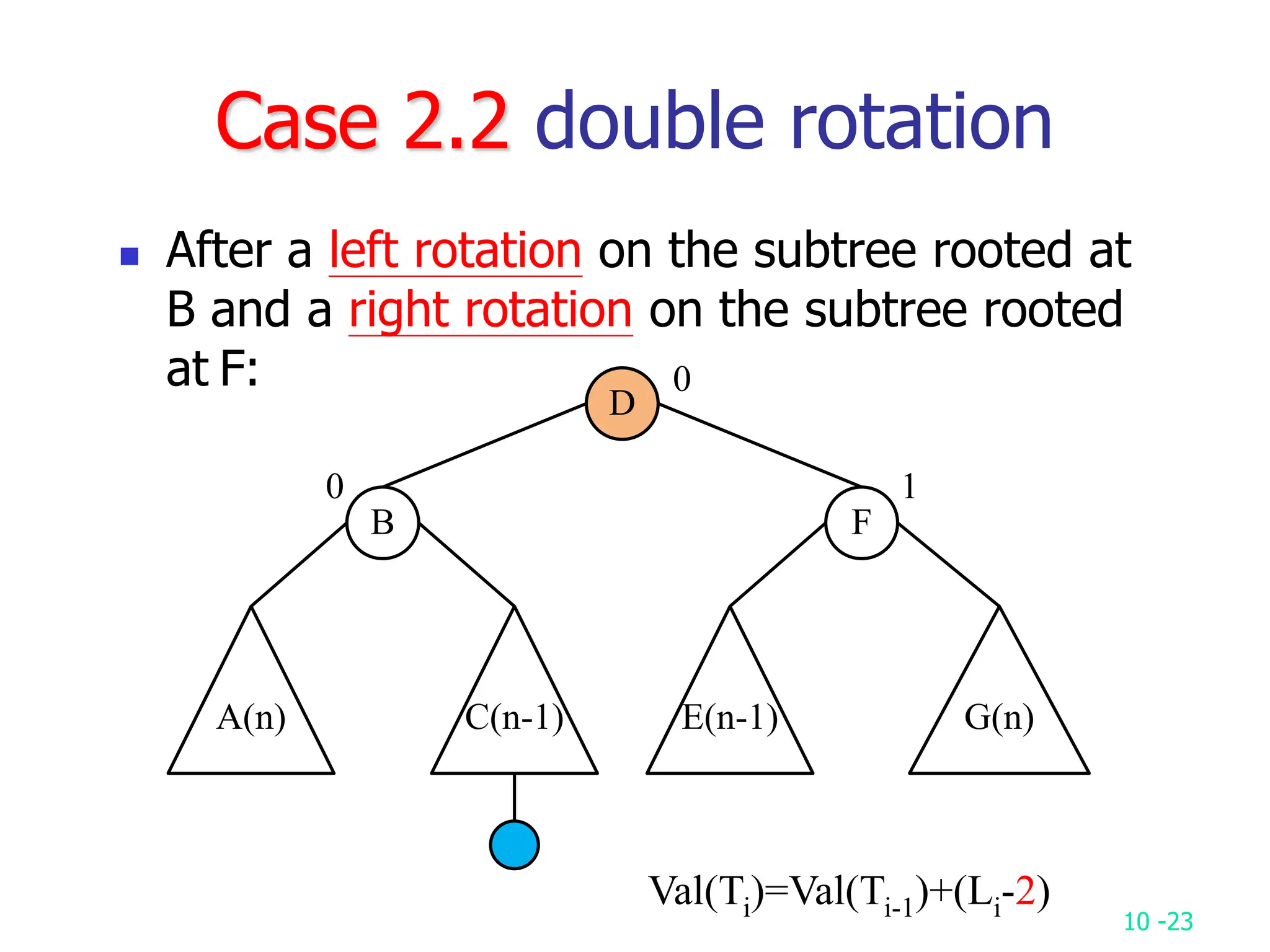
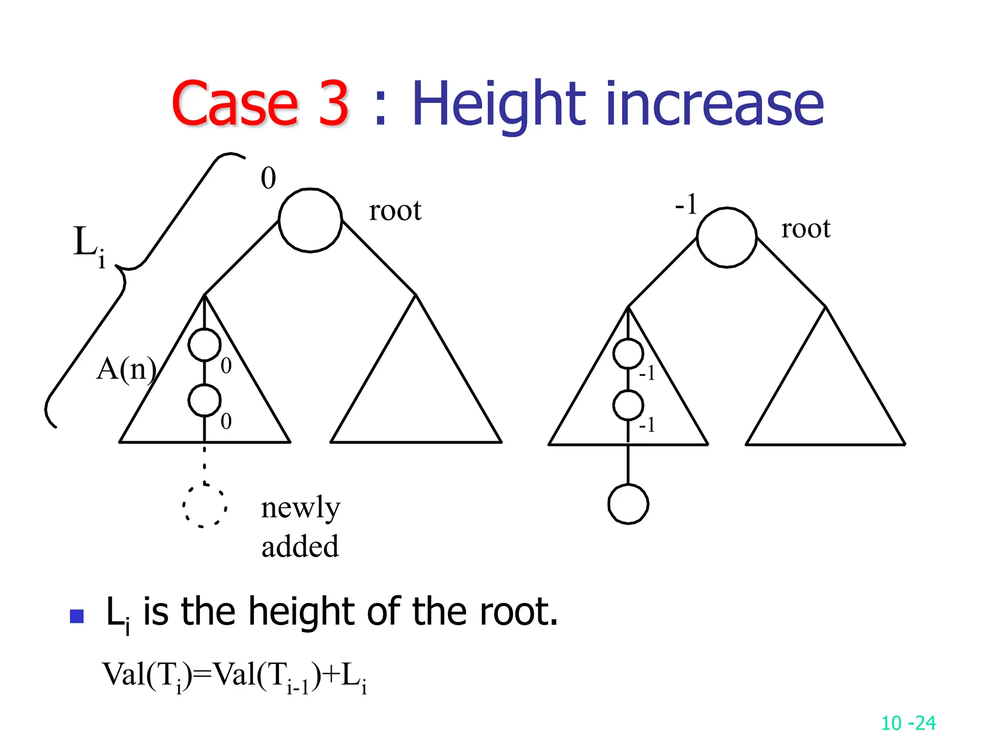
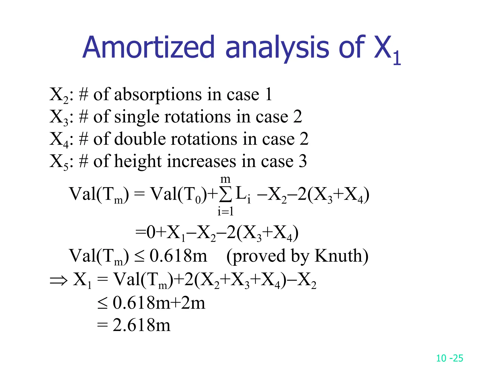
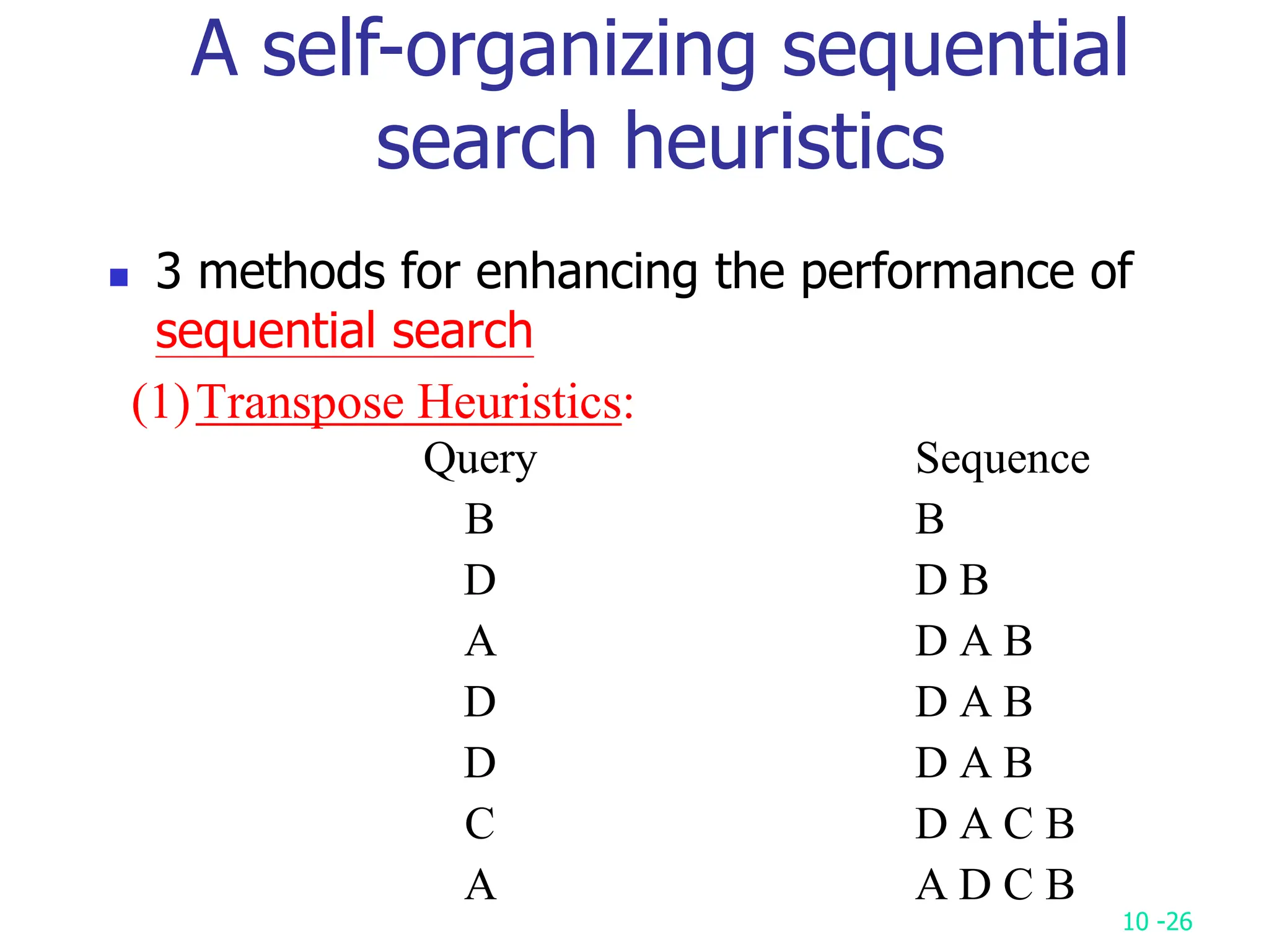
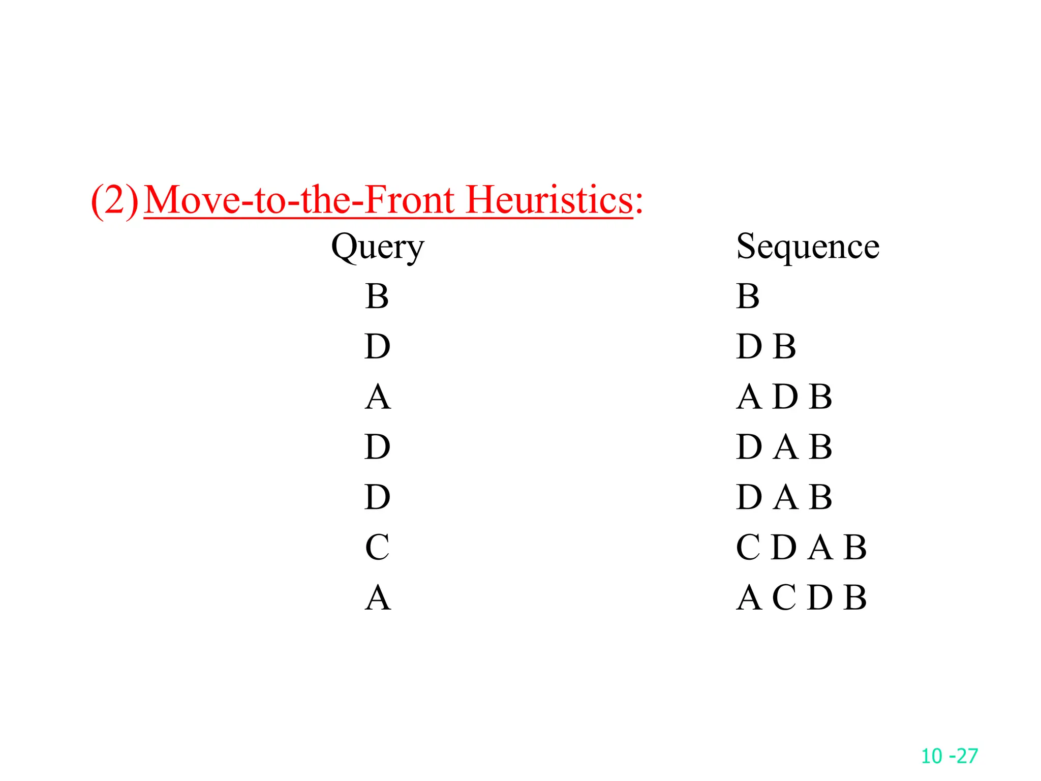
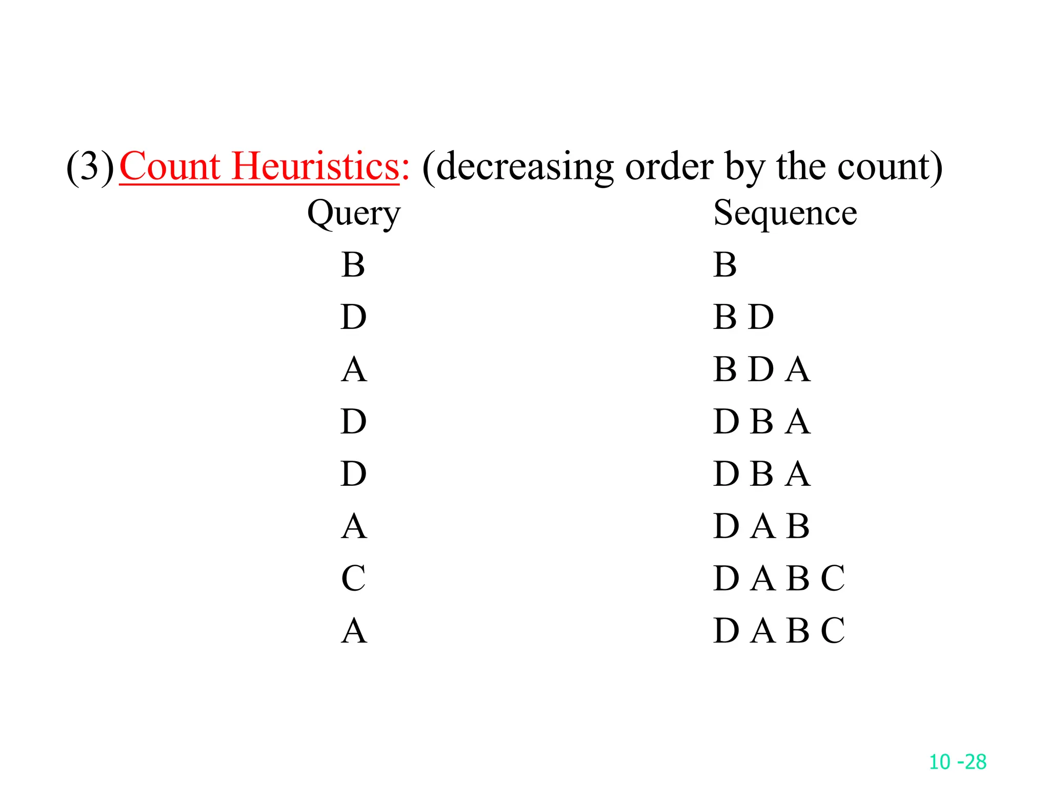
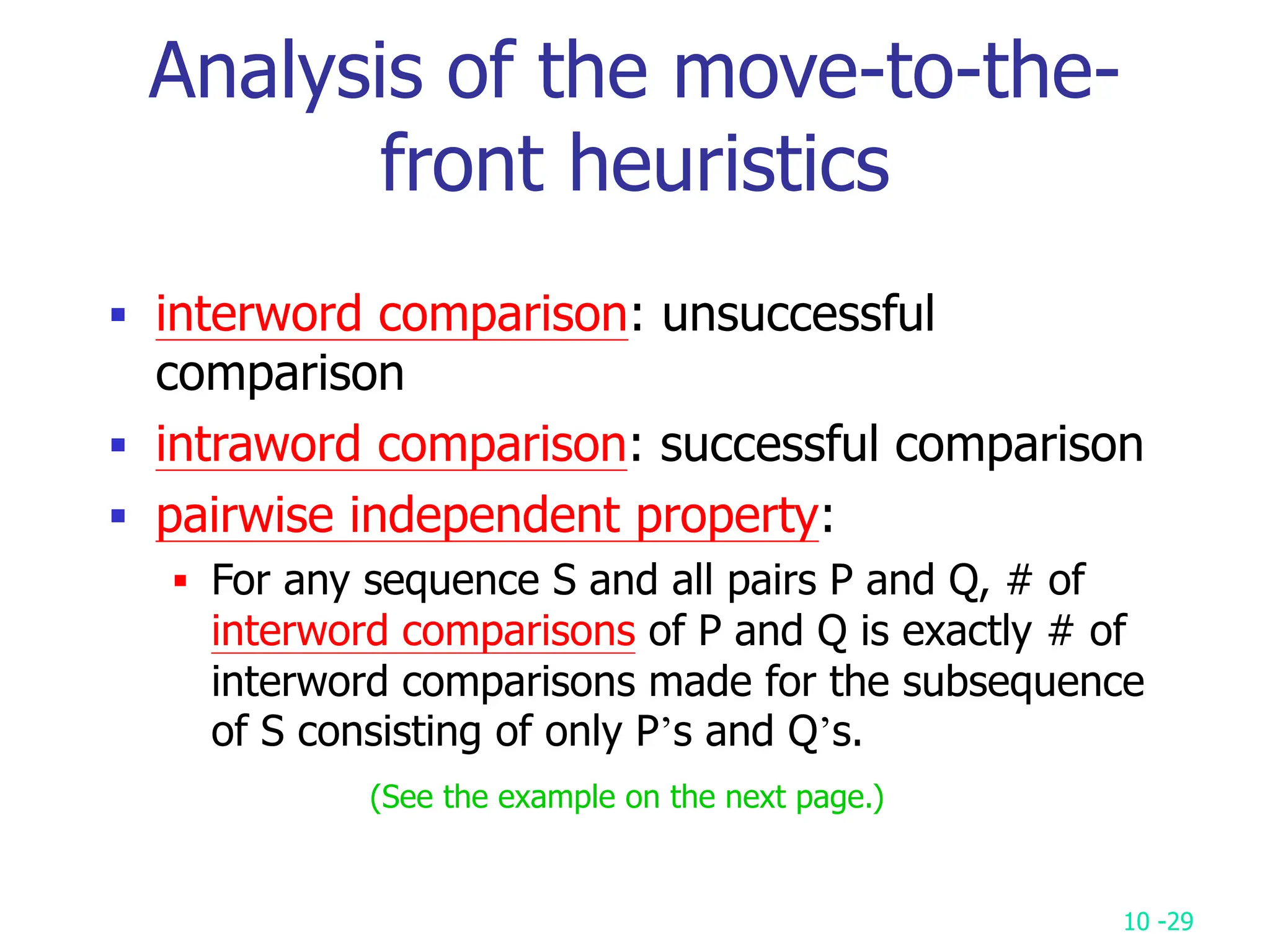
2. It analyzes skew heaps, AVL trees, and several self-organizing sequential search heuristics using amortized analysis. For skew heaps and AVL trees, it defines a potential function to bound the total cost.
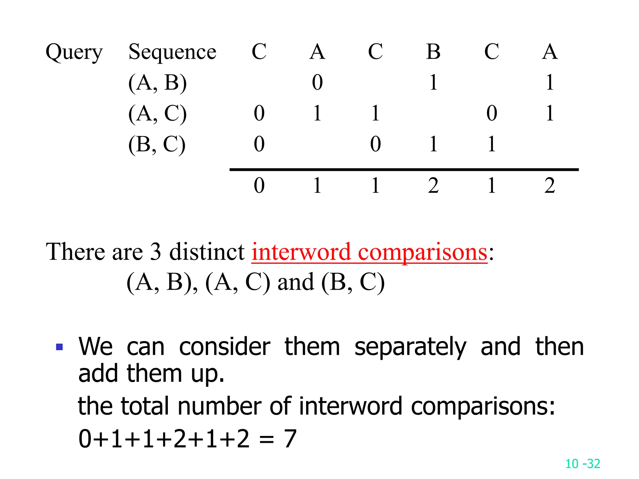
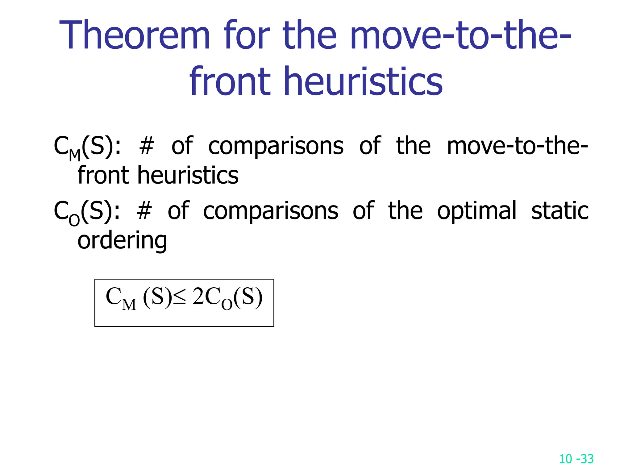
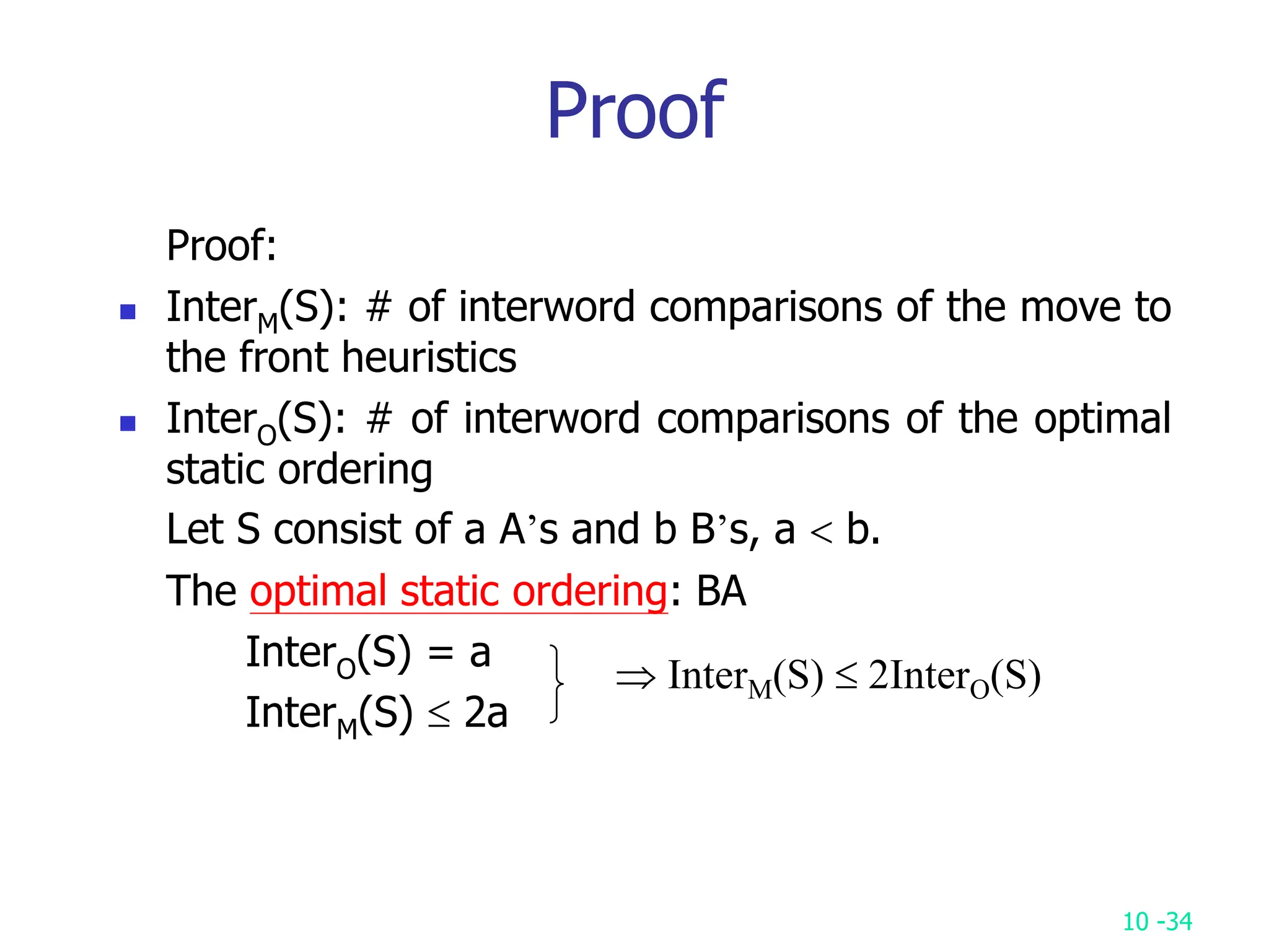
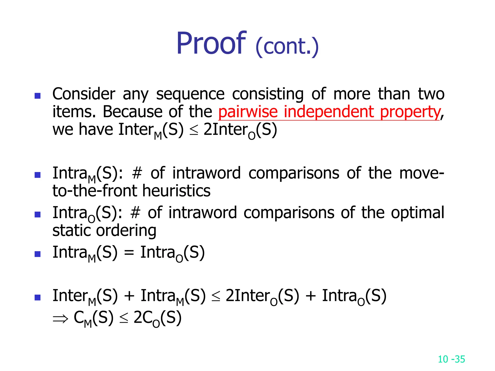
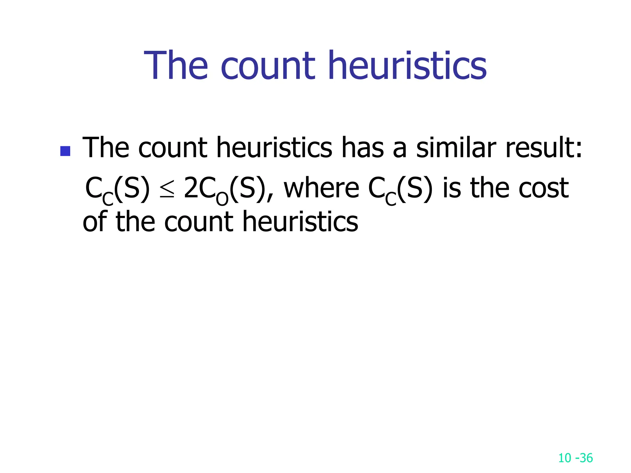
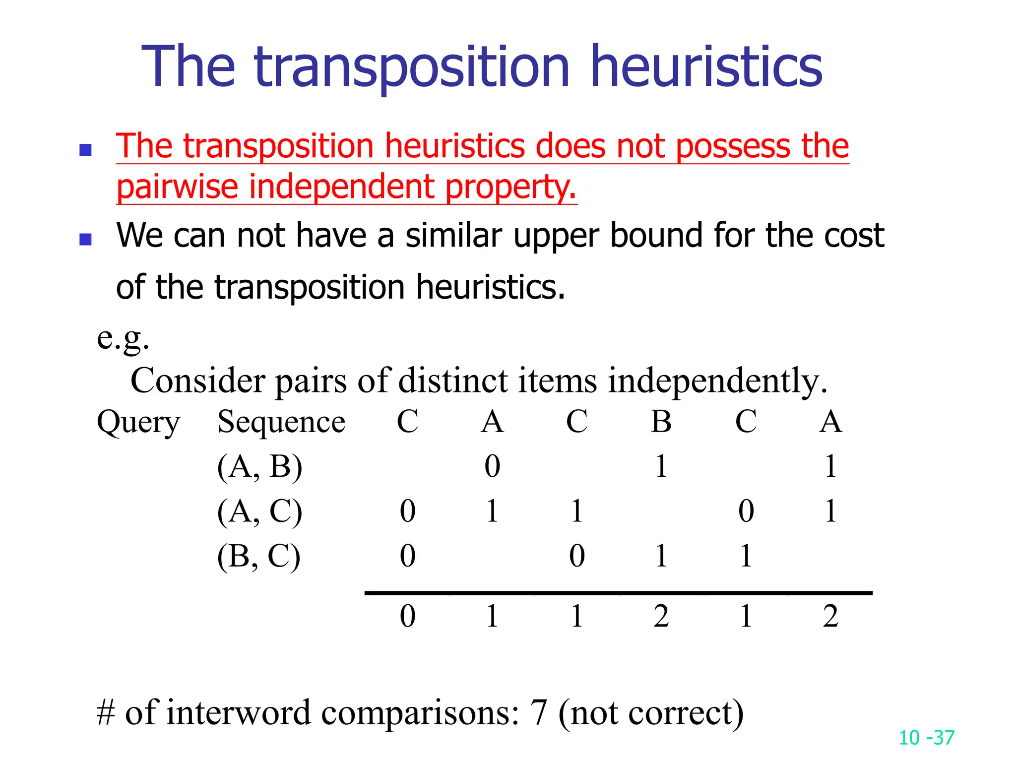
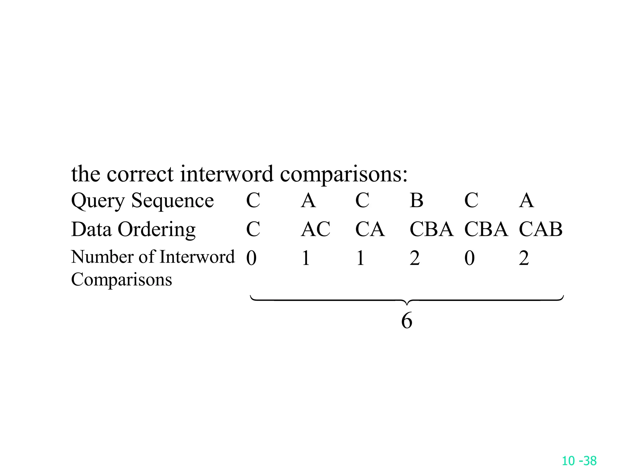
3. It proves that the move-to-front and count heuristics have amortized costs that are at most twice the optimal static ordering, but the transposition heuristic does not have such a