Download to read offline
![UNIT-II
kishore.mamidala@gmail.com
2
UNIT- II
Contents:
Association Rules:
Problem Definition
Frequent Item set Generation
The APRIORI Principle, Support and Confidence Measures,
Association Rule Generation; APRIORI Algorithm,
The Partition Algorithms, FP-Growth Algorithms,
Compact Representation of Frequent Item set – Maximal
Frequent Item set, Closed Frequent Item set.
Mining Frequent Patterns
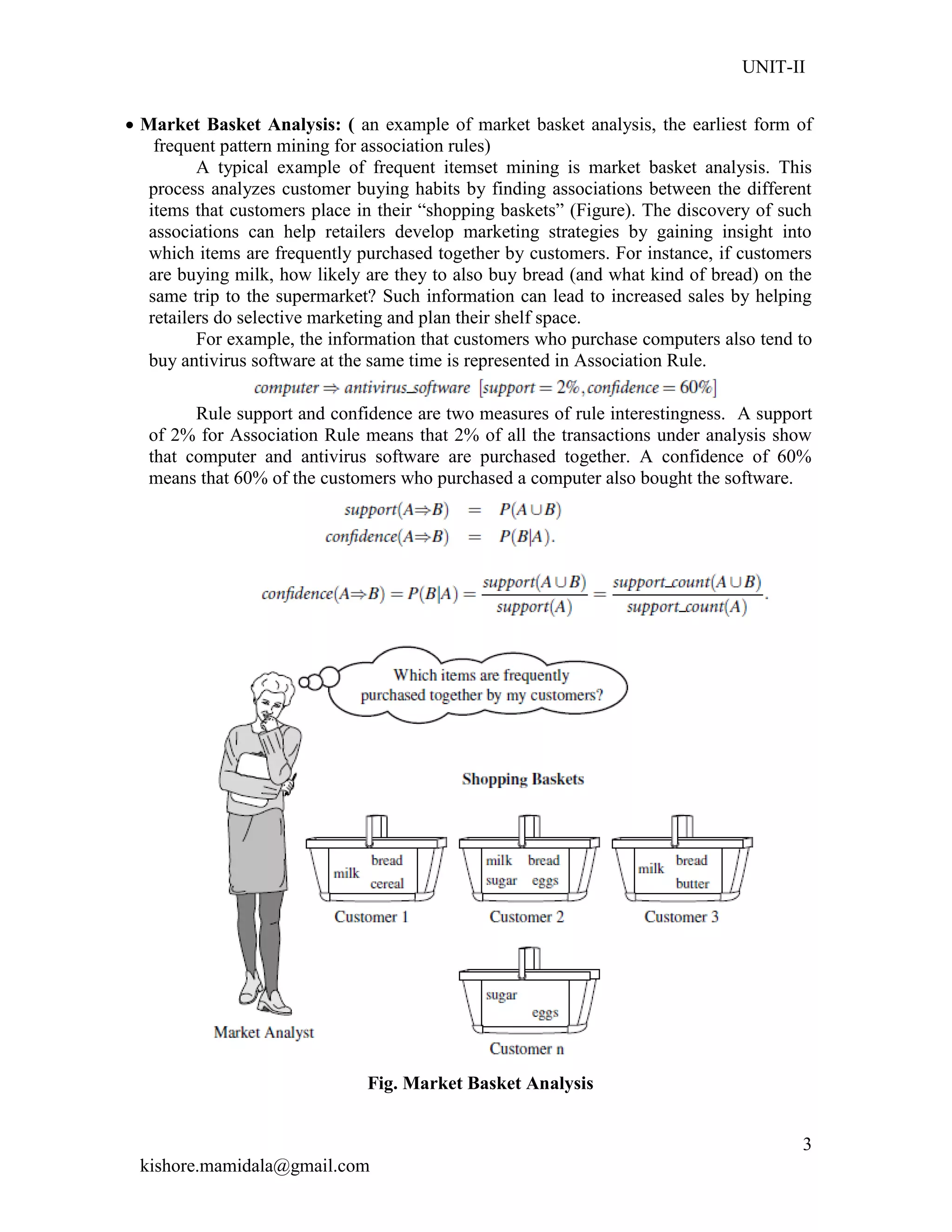
Frequent patterns are patterns (such as itemsets, subsequences, or substructures)
that appear in a data set frequently. For example, a set of items, such as milk and bread,
that appear frequently together in a transaction data set is a frequent itemset. A
subsequence, such as buying first a PC, then a digital camera, and then a memory card, if
it occurs frequently in a shopping history database, is a (frequent) sequential pattern.
Finding such frequent patterns plays an essential role in mining associations,
correlations, and many other interesting relationships among data.
Frequent pattern mining searches for recurring relationships in a given data set.
The basic concepts of frequent pattern mining for the discovery of interesting
associations and correlations between itemsets in transactional and relational databases.
Association rule mining: Finding frequent patterns, associations, correlations, or
causal structures among sets of items or objects in transaction databases, relational
databases, and other information repositories.
―Body -> Head [support, confidence]‖.
Applications:
Basket data analysis, cross-marketing, catalog design, loss-leader analysis,
clustering, classification, etc.
Example.
major(x, ―CS‖) ^ takes(x, ―DB‖) -> grade(x, ―A‖) [1%, 75%]](https://image.slidesharecdn.com/dmunit-iir16-200826020543/75/Dm-unit-ii-r16-2-2048.jpg)

![UNIT-II
kishore.mamidala@gmail.com
2
UNIT- II
Contents:
Association Rules:
Problem Definition
Frequent Item set Generation
The APRIORI Principle, Support and Confidence Measures,
Association Rule Generation; APRIORI Algorithm,
The Partition Algorithms, FP-Growth Algorithms,
Compact Representation of Frequent Item set – Maximal
Frequent Item set, Closed Frequent Item set.
Mining Frequent Patterns
Frequent patterns are patterns (such as itemsets, subsequences, or substructures)
that appear in a data set frequently. For example, a set of items, such as milk and bread,
that appear frequently together in a transaction data set is a frequent itemset. A
subsequence, such as buying first a PC, then a digital camera, and then a memory card, if
it occurs frequently in a shopping history database, is a (frequent) sequential pattern.
Finding such frequent patterns plays an essential role in mining associations,
correlations, and many other interesting relationships among data.
Frequent pattern mining searches for recurring relationships in a given data set.
The basic concepts of frequent pattern mining for the discovery of interesting
associations and correlations between itemsets in transactional and relational databases.
Association rule mining: Finding frequent patterns, associations, correlations, or
causal structures among sets of items or objects in transaction databases, relational
databases, and other information repositories.
―Body -> Head [support, confidence]‖.
Applications:
Basket data analysis, cross-marketing, catalog design, loss-leader analysis,
clustering, classification, etc.
Example.
major(x, ―CS‖) ^ takes(x, ―DB‖) -> grade(x, ―A‖) [1%, 75%]](https://crownmelresort.com/image.slidesharecdn.com/dmunit-iir16-200826020543/75/Dm-unit-ii-r16-2-2048.jpg)


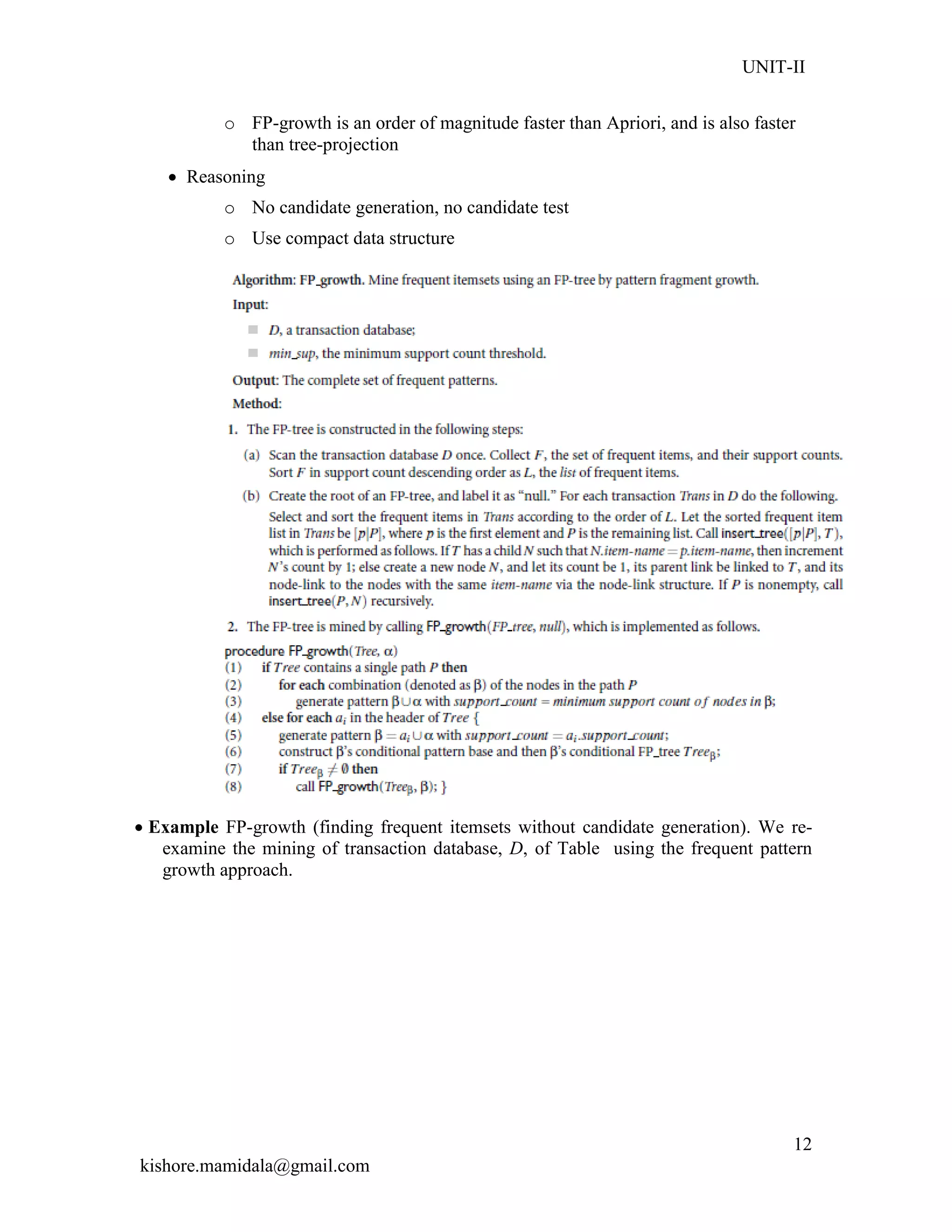
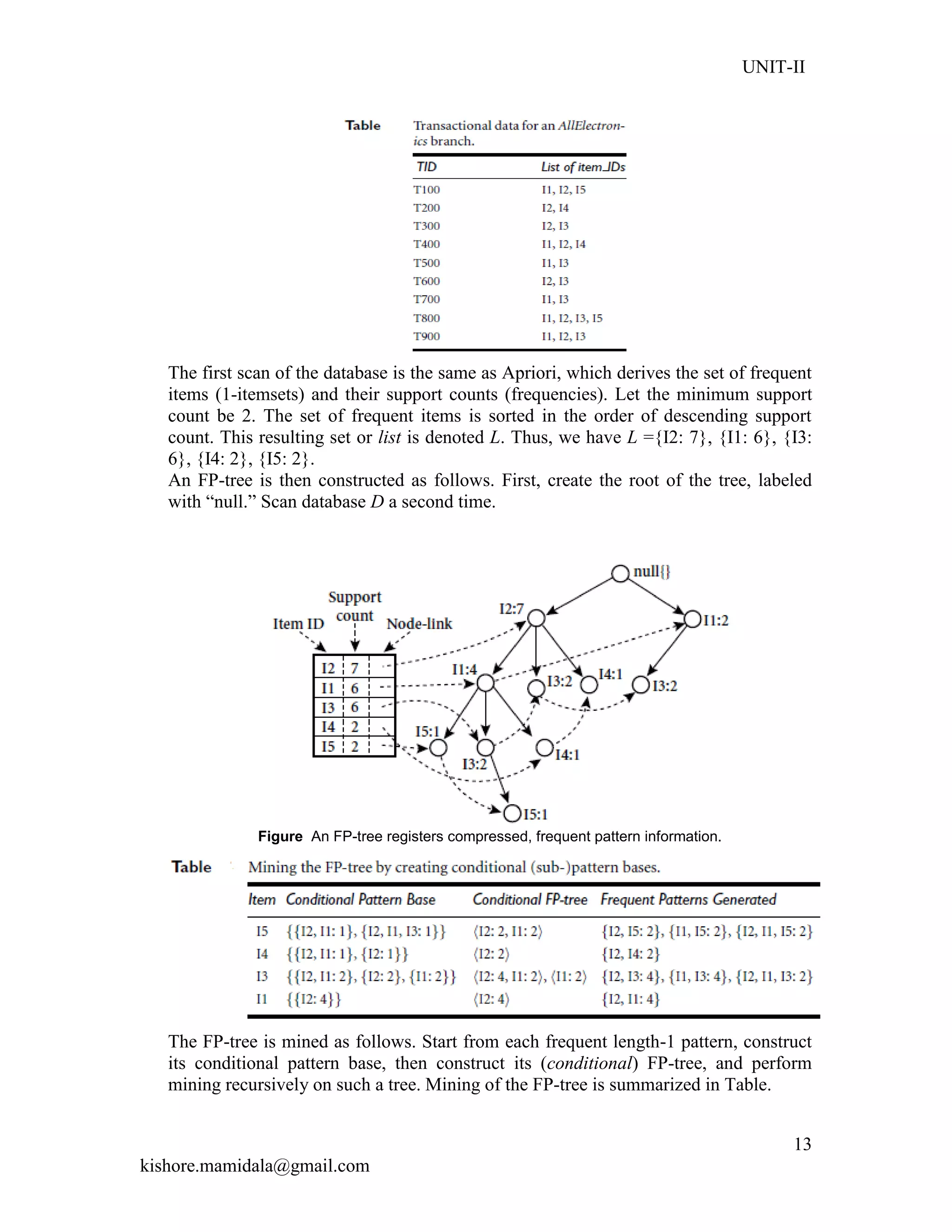
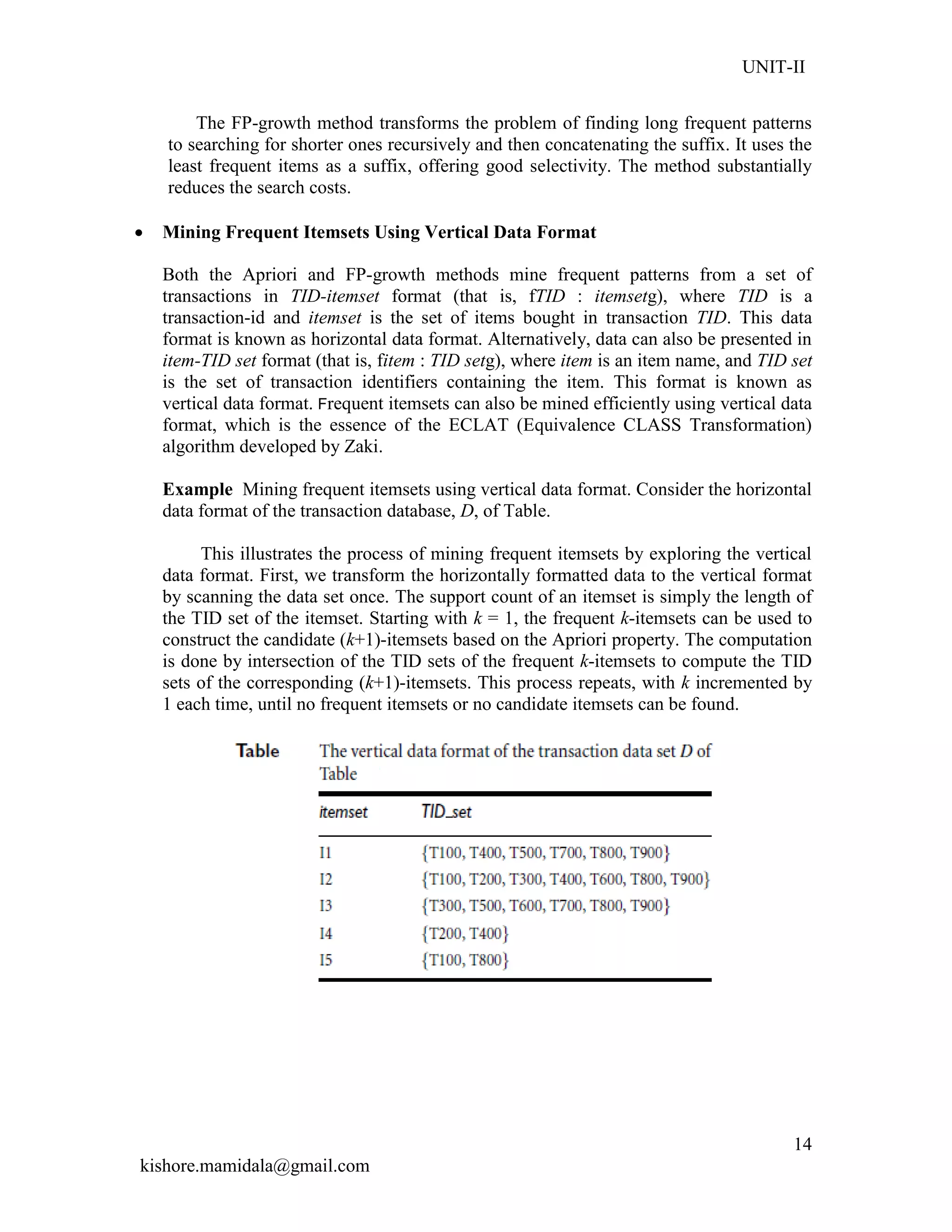
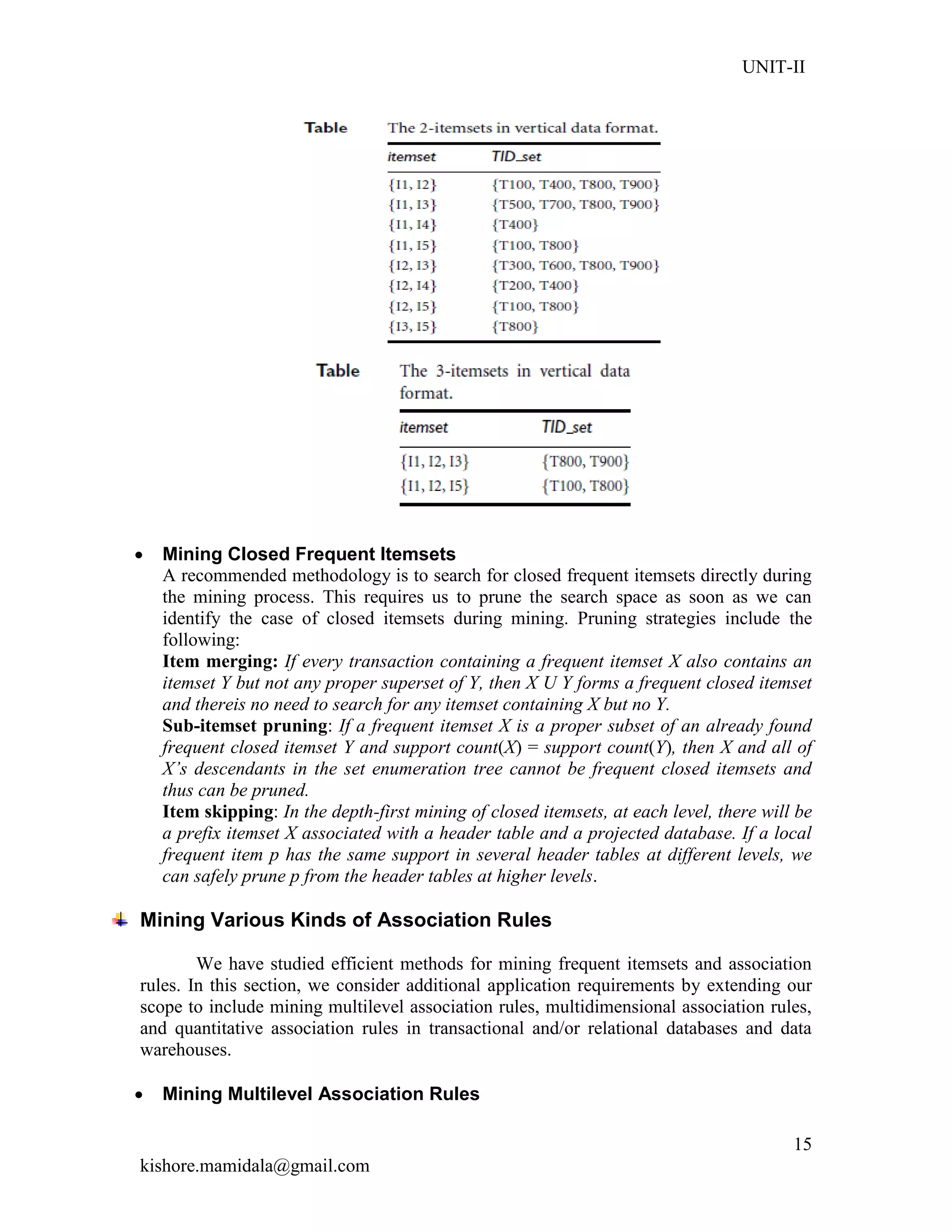
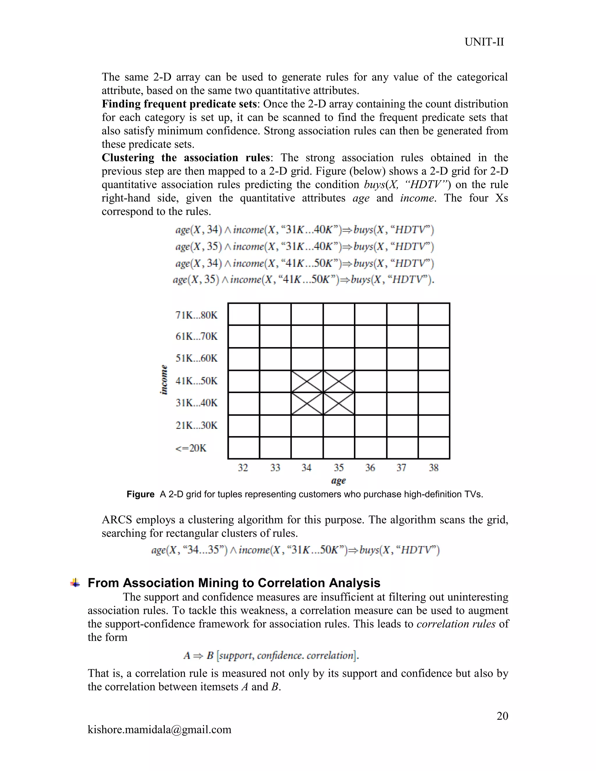
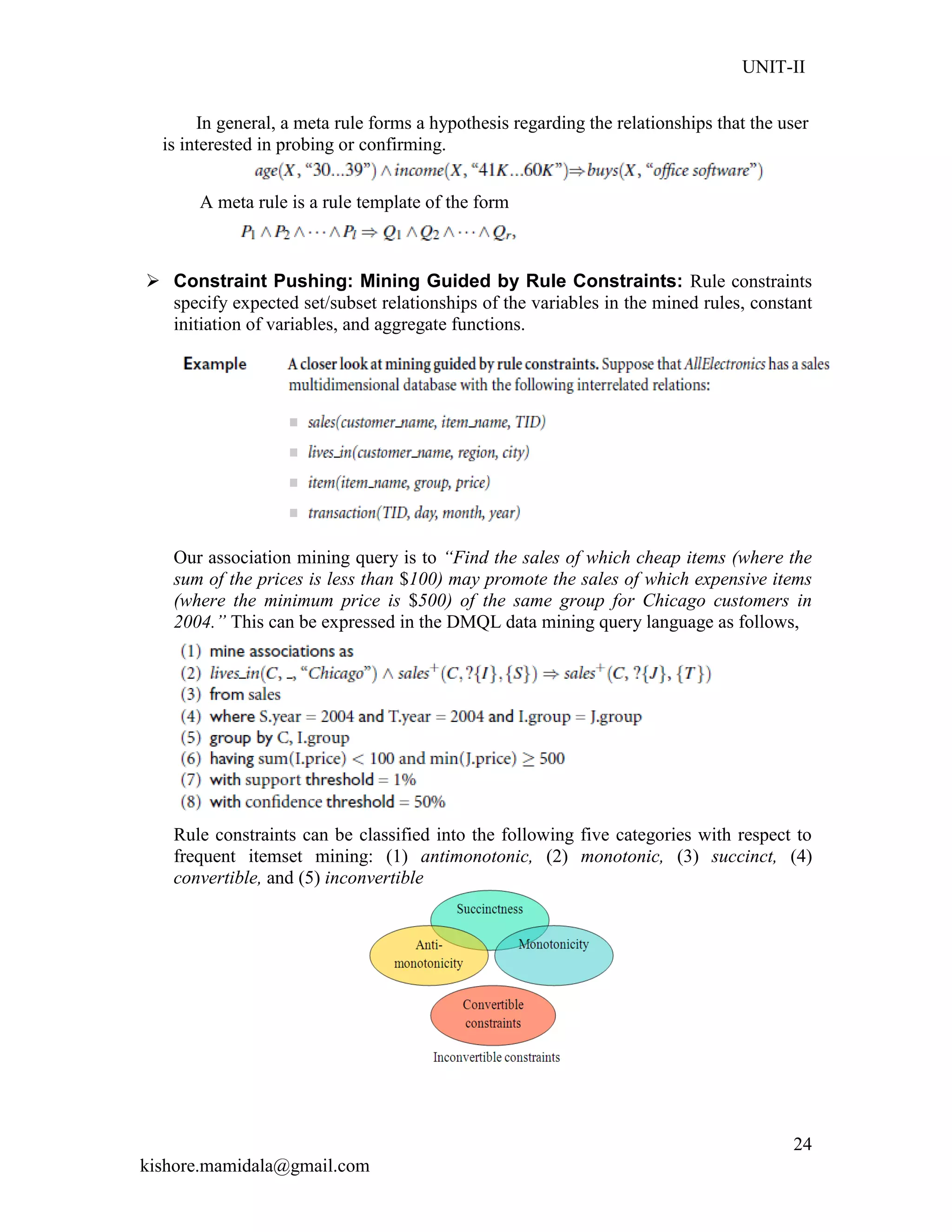
This document discusses frequent pattern mining and association rule mining. It begins by defining frequent patterns as patterns that appear frequently in a dataset, such as frequently purchased itemsets. It then describes the Apriori algorithm for finding frequent itemsets, which uses multiple passes over the data and candidate generation. The document also introduces FP-Growth, an alternative algorithm that avoids candidate generation by compressing the database into a frequent-pattern tree. Finally, it discusses generating association rules from frequent itemsets and techniques for improving the efficiency of frequent pattern mining.