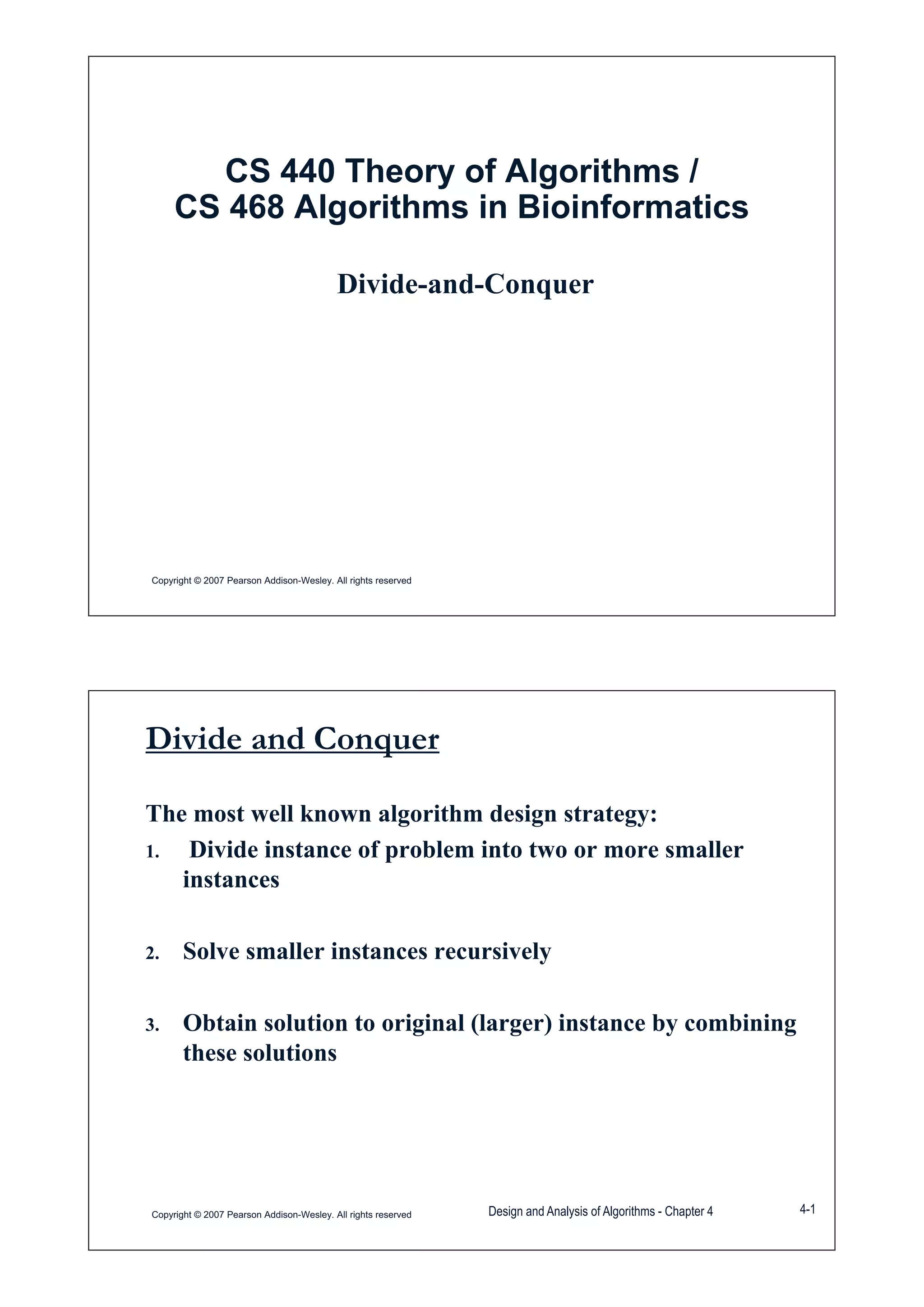
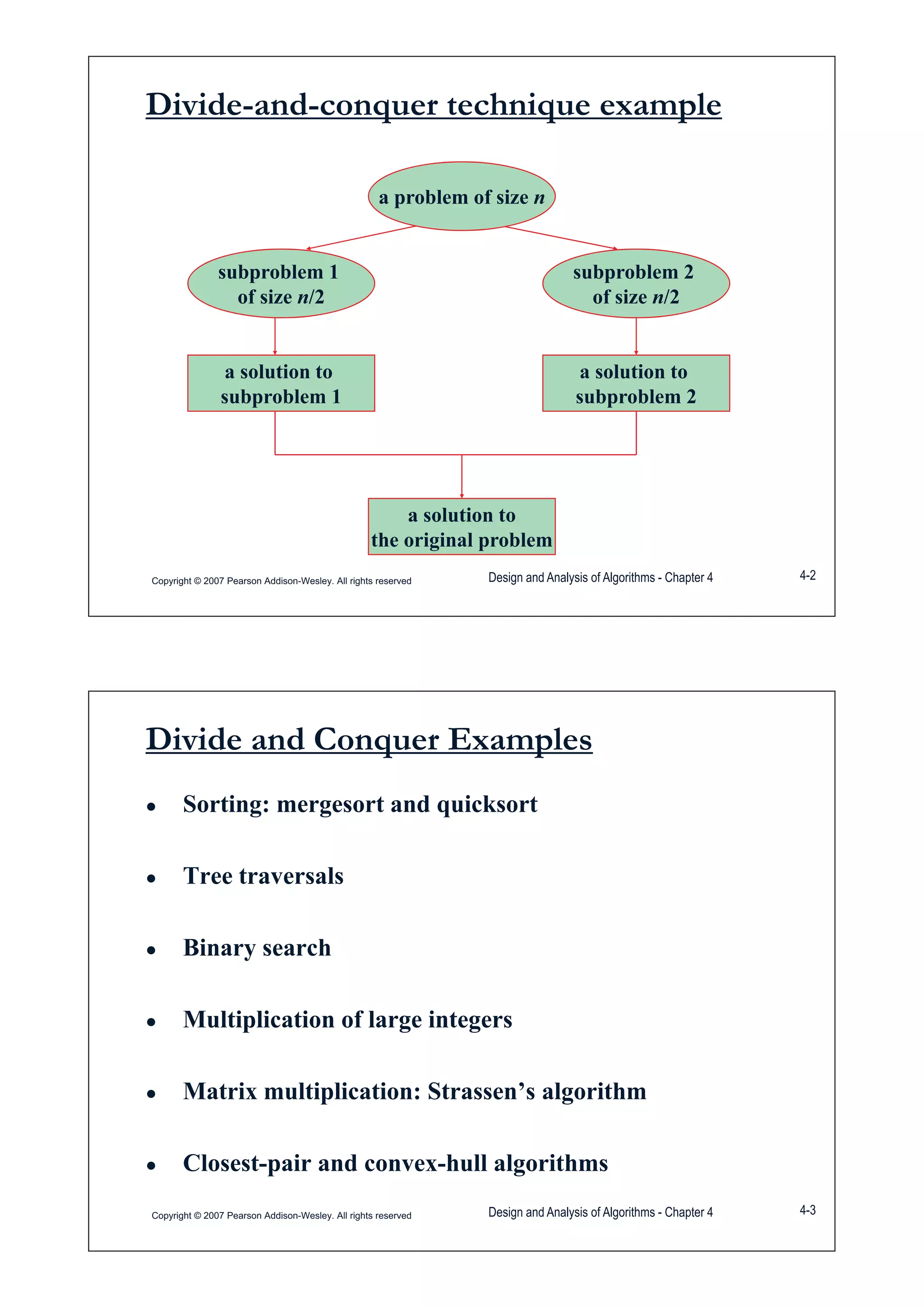
This document discusses the divide-and-conquer algorithm design strategy. It begins by defining divide-and-conquer as dividing a problem into smaller subproblems, solving those subproblems recursively, and combining the solutions. Examples covered include sorting algorithms like mergesort and quicksort, tree traversals, binary search, integer multiplication, matrix multiplication using Strassen's algorithm, and closest pair problems. Analysis techniques like recursion trees and the master theorem are introduced.
![General Divide and Conquer recurrence:
T(n) = aT(n/b) + f (n) where f (n) Ĭ(nd)T(n) aT(n/b) + f (n) where f (n) Ĭ(n )
Master Theorem
d d• a < bd T(n) Ĭ(nd)
• a = bd T(n) Ĭ(nd lg n )
• a > bd T(n) Ĭ(nlog b a)
Note: the same results hold with O instead of Ĭ.Note: the same results hold with O instead of Ĭ.
Examples: T(n) = 4T(n/3) + n Ÿ T(n) ?Examples: T(n) 4T(n/3) + n Ÿ T(n) ?
T(n) = 2T(n/2) + n2 Ÿ T(n) ?
T(n) = 8T(n/2) + n3 Ÿ T(n) ?
Copyright © 2007 Pearson Addison-Wesley. All rights reserved Design and Analysis of Algorithms - Chapter 4 4-4
T(n) = 8T(n/2) + n Ÿ T(n) ?
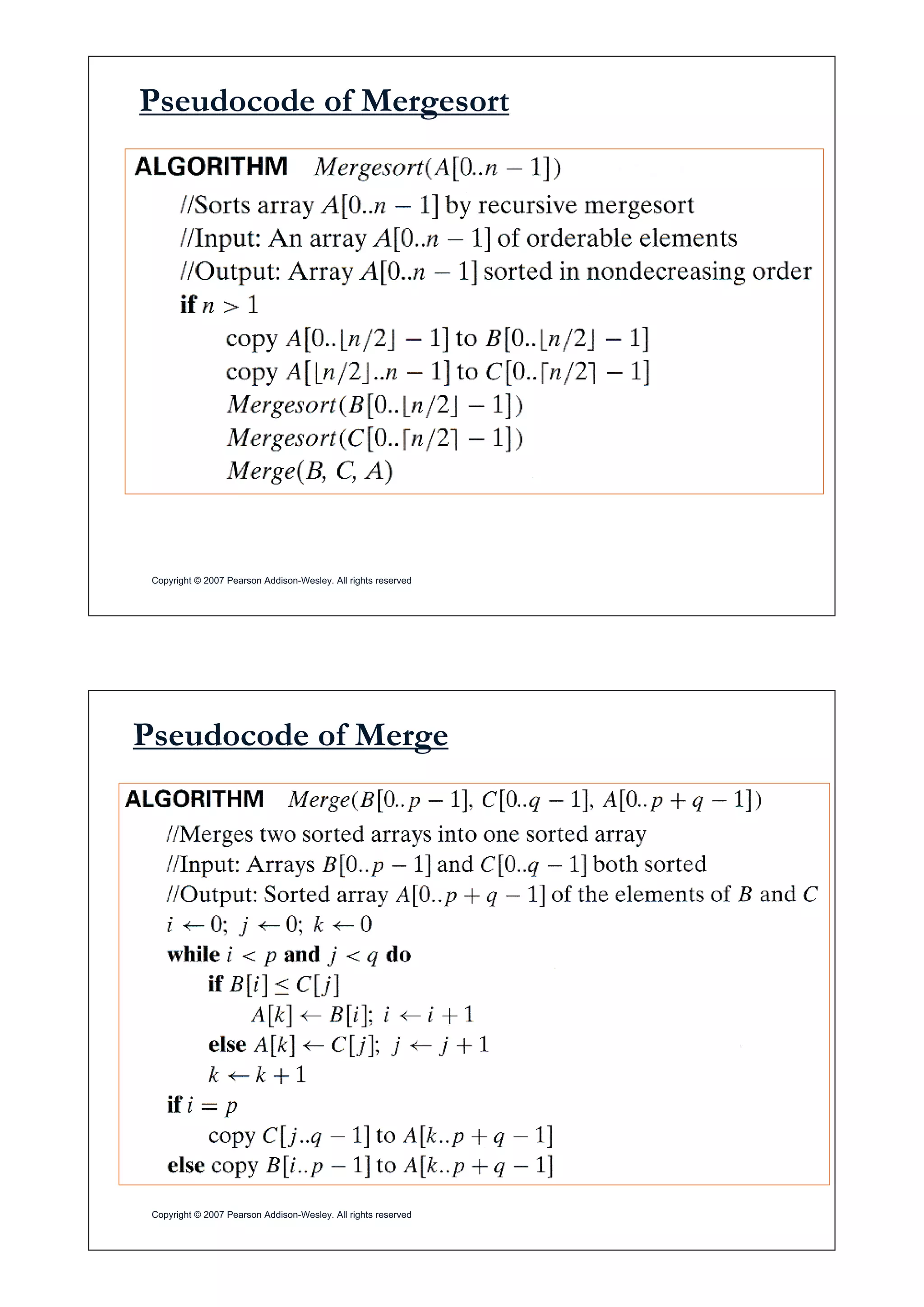
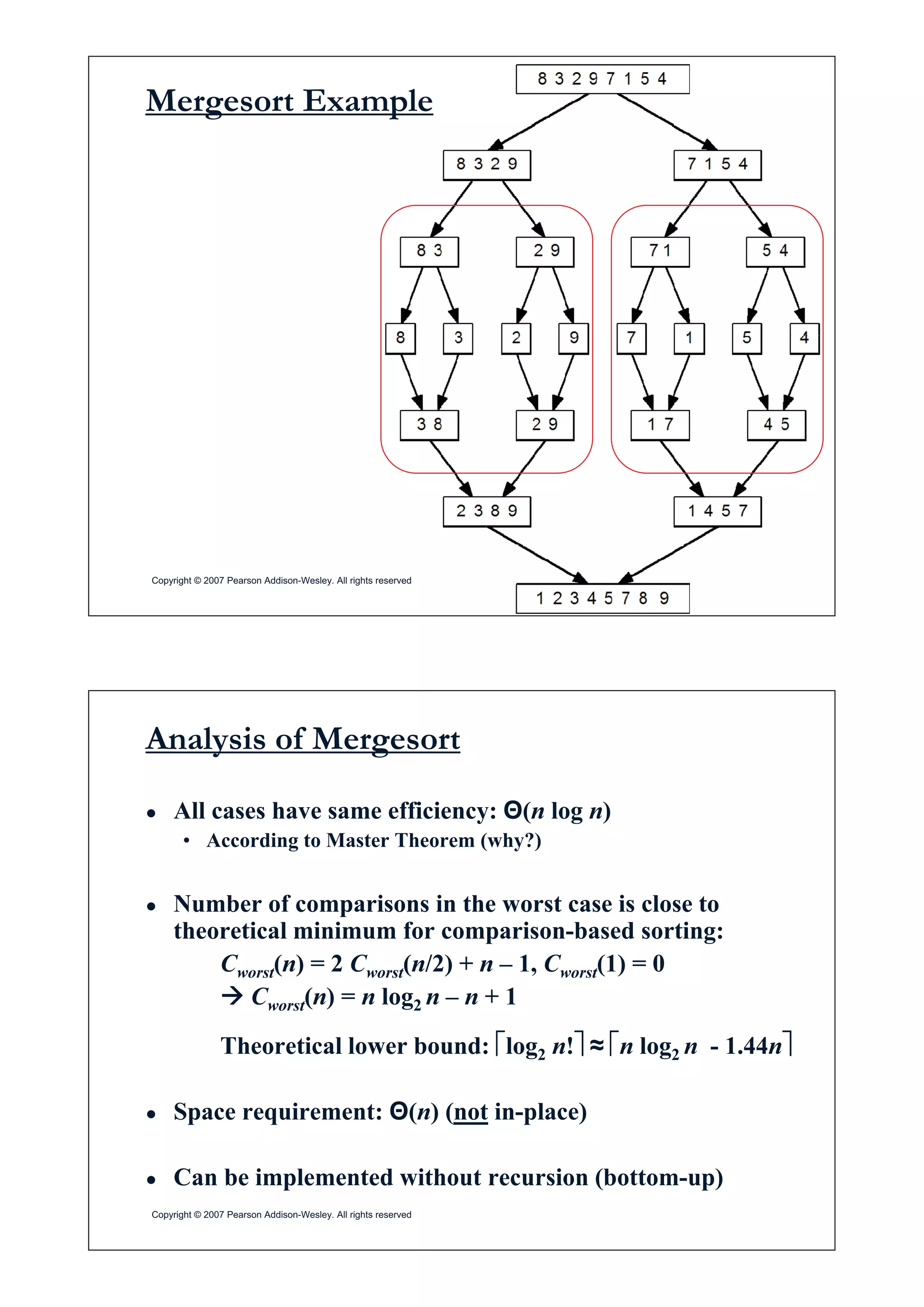
Mergesort
Ɣ Split array A[0..n-1] in two about equal halves and make
copies of each half in arrays B and Ccopies of each half in arrays B and C
Ɣ Sort arrays B and C recursively
Ɣ Merge sorted arrays B and C into array A as follows:Ɣ Merge sorted arrays B and C into array A as follows:
• Repeat the following until no elements remain in one of
the arrays:y
– compare the first elements in the remaining
unprocessed portions of the arrays
– copy the smaller of the two into A, while
incrementing the index indicating the unprocessed
portion of that arrayportion of that array
• Once all elements in one of the arrays are processed,
copy the remaining unprocessed elements from the other
Copyright © 2007 Pearson Addison-Wesley. All rights reserved
array into A.](https://image.slidesharecdn.com/divideandconquer-190317183448/75/Divide-and-conquer-3-2048.jpg)
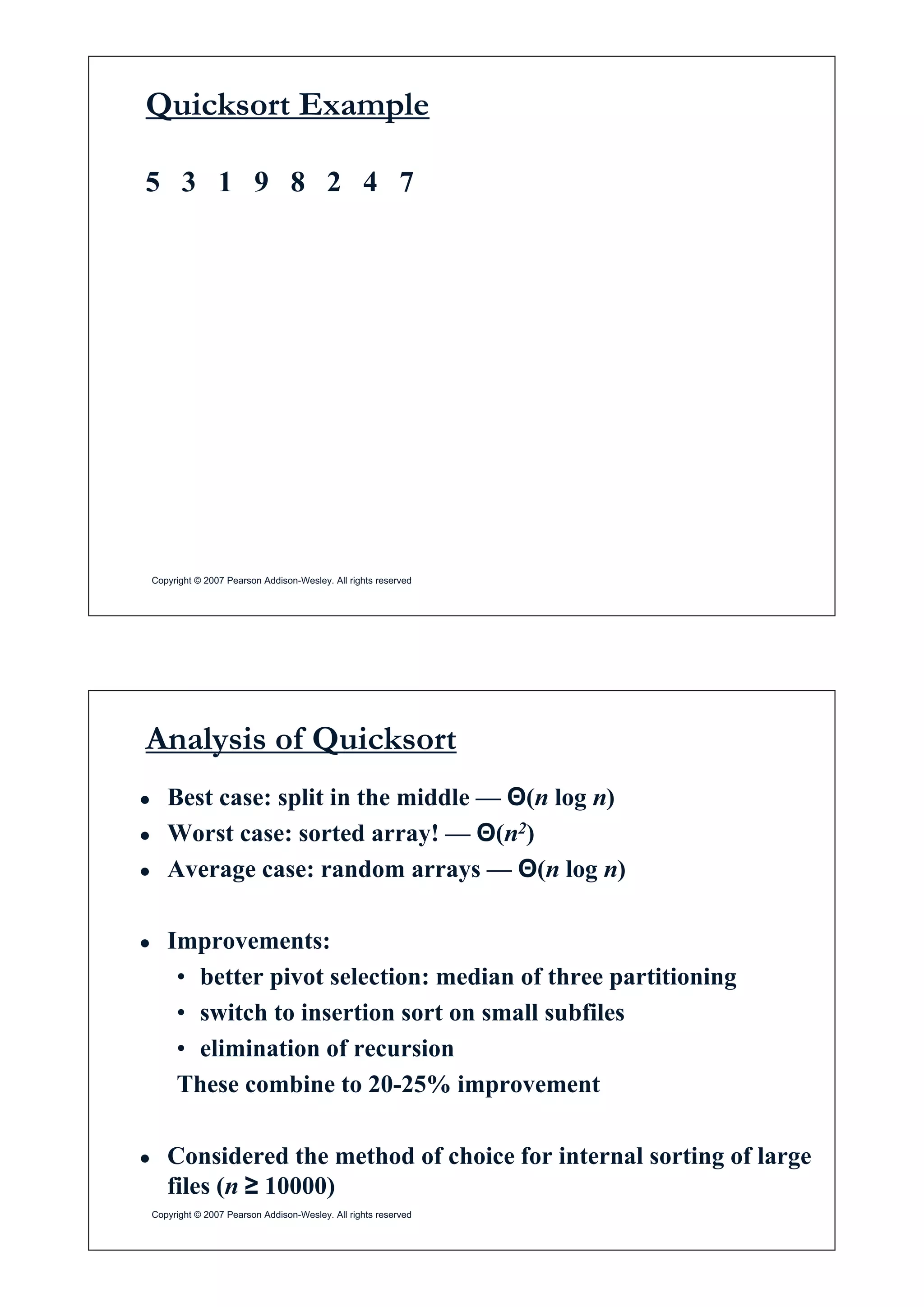
![Quicksort
Ɣ Select a pivot (partitioning element) – here, the first element
Ɣ Rearrange the list so that all the elements in the first s
positions are smaller than or equal to the pivot and all the
i i i i ielements in the remaining n-s positions are larger than or
equal to the pivot (see next slide for an algorithm)
p
A[i]dp A[i]tp
Ɣ Exchange the pivot with the last element in the first (i.e., d)
subarray — the pivot is now in its final position
Copyright © 2007 Pearson Addison-Wesley. All rights reserved
Ɣ Sort the two subarrays recursively
Partitioning Algorithm
dd
The index i can
go out of thego out of the
subarray bound
and it needs to
Copyright © 2007 Pearson Addison-Wesley. All rights reserved
be taken care of.](https://image.slidesharecdn.com/divideandconquer-190317183448/75/Divide-and-conquer-6-2048.jpg)
![Binary Search
Very efficient algorithm for searching in sorted array:
K
vs
A[0] . . . A[m] . . . A[n-1]
If K = A[m], stop (successful search); otherwise, continue
searching by the same method in A[0..m-1] if K < A[m]
and in A[m+1 n 1] if K > A[m]and in A[m+1..n-1] if K > A[m]
l m 0; r m n-1
while l d r do
m m ¬(l+r)/2¼
if K = A[m] return mif K = A[m] return m
else if K < A[m] r m m-1
else l m m+1
Copyright © 2007 Pearson Addison-Wesley. All rights reserved
return -1
Analysis of Binary Search
Ɣ Time efficiency
• worst-case recurrence: Cw (n) = 1 + Cw( ¬n/2¼ ), Cw (1) = 1w ( ) w( ¬ ¼ ), w ( )
solution: Cw(n) = ªlog2(n+1)º
This is VERY fast: e g C (106) = 20This is VERY fast: e.g., Cw(106) = 20
Ɣ Optimal for searching a sorted arrayp g y
Ɣ Limitations: must be a sorted array (not linked list)
Ɣ Degenerate example of divide-and-conquer
Copyright © 2007 Pearson Addison-Wesley. All rights reserved](https://image.slidesharecdn.com/divideandconquer-190317183448/75/Divide-and-conquer-8-2048.jpg)
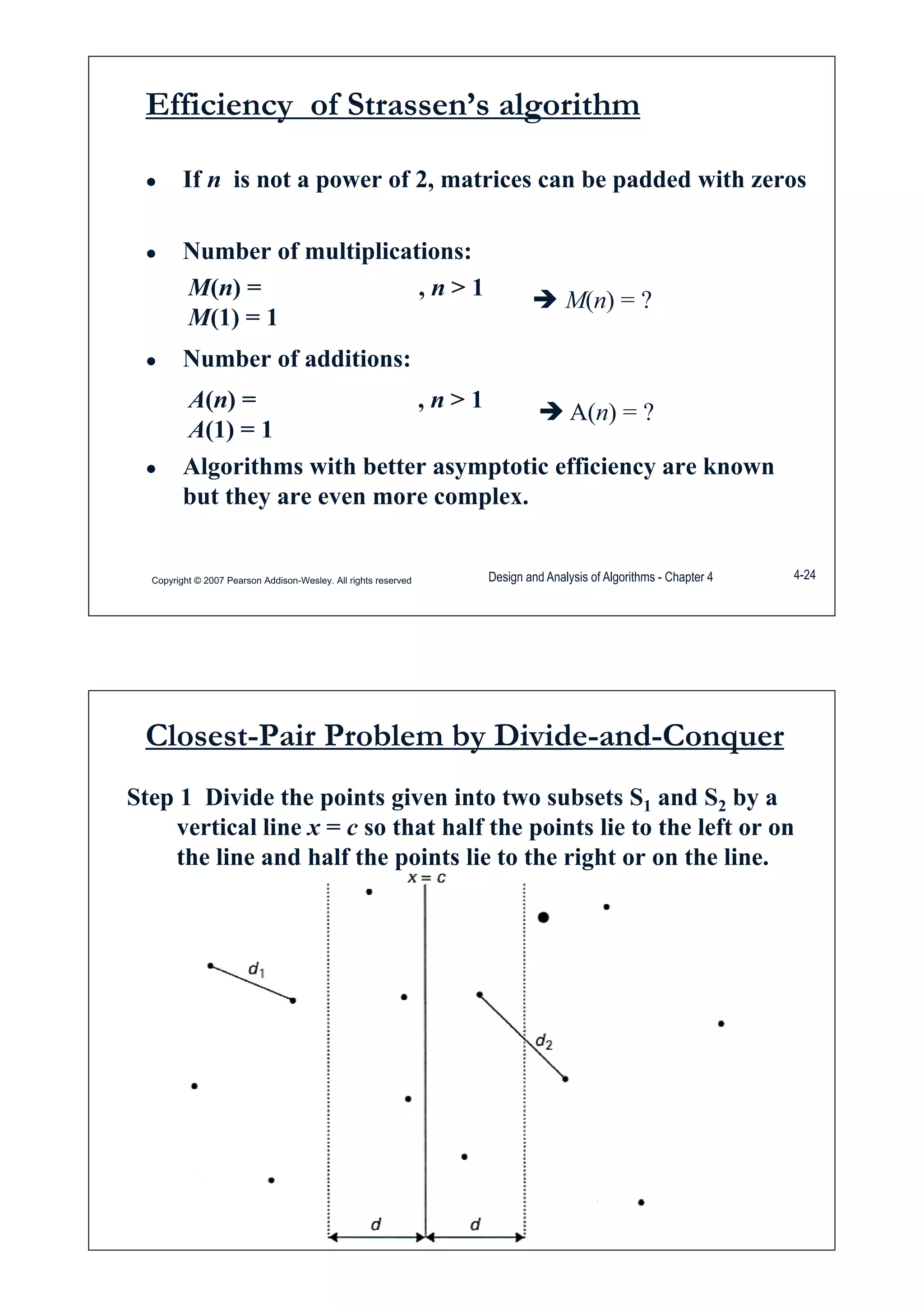
![Strassen’s matrix multiplication
Ɣ Strassen observed [1969] that the product of two matrices
can be computed as follows:
C00 C01 A00 A01 B00 B01
= *
C C A A B BC10 C11 A10 A11 B10 B11
M + M M + M M + MM1 + M4 - M5 + M7 M3 + M5
=
M2 + M4 M1 + M3 - M2 + M62 4 1 3 2 6
Copyright © 2007 Pearson Addison-Wesley. All rights reserved Design and Analysis of Algorithms - Chapter 4 4-22
Submatrices:
Ɣ M1 = (A00 + A11) * (B00 + B11)
Ɣ M2 = (A10 + A11) * B00
Ɣ M3 = A00 * (B01 - B11)
M = A * (B B )Ɣ M4 = A11 * (B10 - B00)
Ɣ M5 = (A00 + A01) * B11
Ɣ M6 = (A10 - A00) * (B00 + B01)
Ɣ M7 = (A01 - A11) * (B10 + B11)
Copyright © 2007 Pearson Addison-Wesley. All rights reserved Design and Analysis of Algorithms - Chapter 4 4-23](https://image.slidesharecdn.com/divideandconquer-190317183448/75/Divide-and-conquer-12-2048.jpg)


![General Divide and Conquer recurrence:
T(n) = aT(n/b) + f (n) where f (n) Ĭ(nd)T(n) aT(n/b) + f (n) where f (n) Ĭ(n )
Master Theorem
d d• a < bd T(n) Ĭ(nd)
• a = bd T(n) Ĭ(nd lg n )
• a > bd T(n) Ĭ(nlog b a)
Note: the same results hold with O instead of Ĭ.Note: the same results hold with O instead of Ĭ.
Examples: T(n) = 4T(n/3) + n Ÿ T(n) ?Examples: T(n) 4T(n/3) + n Ÿ T(n) ?
T(n) = 2T(n/2) + n2 Ÿ T(n) ?
T(n) = 8T(n/2) + n3 Ÿ T(n) ?
Copyright © 2007 Pearson Addison-Wesley. All rights reserved Design and Analysis of Algorithms - Chapter 4 4-4
T(n) = 8T(n/2) + n Ÿ T(n) ?
Mergesort
Ɣ Split array A[0..n-1] in two about equal halves and make
copies of each half in arrays B and Ccopies of each half in arrays B and C
Ɣ Sort arrays B and C recursively
Ɣ Merge sorted arrays B and C into array A as follows:Ɣ Merge sorted arrays B and C into array A as follows:
• Repeat the following until no elements remain in one of
the arrays:y
– compare the first elements in the remaining
unprocessed portions of the arrays
– copy the smaller of the two into A, while
incrementing the index indicating the unprocessed
portion of that arrayportion of that array
• Once all elements in one of the arrays are processed,
copy the remaining unprocessed elements from the other
Copyright © 2007 Pearson Addison-Wesley. All rights reserved
array into A.](https://crownmelresort.com/image.slidesharecdn.com/divideandconquer-190317183448/75/Divide-and-conquer-3-2048.jpg)


![Quicksort
Ɣ Select a pivot (partitioning element) – here, the first element
Ɣ Rearrange the list so that all the elements in the first s
positions are smaller than or equal to the pivot and all the
i i i i ielements in the remaining n-s positions are larger than or
equal to the pivot (see next slide for an algorithm)
p
A[i]dp A[i]tp
Ɣ Exchange the pivot with the last element in the first (i.e., d)
subarray — the pivot is now in its final position
Copyright © 2007 Pearson Addison-Wesley. All rights reserved
Ɣ Sort the two subarrays recursively
Partitioning Algorithm
dd
The index i can
go out of thego out of the
subarray bound
and it needs to
Copyright © 2007 Pearson Addison-Wesley. All rights reserved
be taken care of.](https://crownmelresort.com/image.slidesharecdn.com/divideandconquer-190317183448/75/Divide-and-conquer-6-2048.jpg)

![Binary Search
Very efficient algorithm for searching in sorted array:
K
vs
A[0] . . . A[m] . . . A[n-1]
If K = A[m], stop (successful search); otherwise, continue
searching by the same method in A[0..m-1] if K < A[m]
and in A[m+1 n 1] if K > A[m]and in A[m+1..n-1] if K > A[m]
l m 0; r m n-1
while l d r do
m m ¬(l+r)/2¼
if K = A[m] return mif K = A[m] return m
else if K < A[m] r m m-1
else l m m+1
Copyright © 2007 Pearson Addison-Wesley. All rights reserved
return -1
Analysis of Binary Search
Ɣ Time efficiency
• worst-case recurrence: Cw (n) = 1 + Cw( ¬n/2¼ ), Cw (1) = 1w ( ) w( ¬ ¼ ), w ( )
solution: Cw(n) = ªlog2(n+1)º
This is VERY fast: e g C (106) = 20This is VERY fast: e.g., Cw(106) = 20
Ɣ Optimal for searching a sorted arrayp g y
Ɣ Limitations: must be a sorted array (not linked list)
Ɣ Degenerate example of divide-and-conquer
Copyright © 2007 Pearson Addison-Wesley. All rights reserved](https://crownmelresort.com/image.slidesharecdn.com/divideandconquer-190317183448/75/Divide-and-conquer-8-2048.jpg)


![Strassen’s matrix multiplication
Ɣ Strassen observed [1969] that the product of two matrices
can be computed as follows:
C00 C01 A00 A01 B00 B01
= *
C C A A B BC10 C11 A10 A11 B10 B11
M + M M + M M + MM1 + M4 - M5 + M7 M3 + M5
=
M2 + M4 M1 + M3 - M2 + M62 4 1 3 2 6
Copyright © 2007 Pearson Addison-Wesley. All rights reserved Design and Analysis of Algorithms - Chapter 4 4-22
Submatrices:
Ɣ M1 = (A00 + A11) * (B00 + B11)
Ɣ M2 = (A10 + A11) * B00
Ɣ M3 = A00 * (B01 - B11)
M = A * (B B )Ɣ M4 = A11 * (B10 - B00)
Ɣ M5 = (A00 + A01) * B11
Ɣ M6 = (A10 - A00) * (B00 + B01)
Ɣ M7 = (A01 - A11) * (B10 + B11)
Copyright © 2007 Pearson Addison-Wesley. All rights reserved Design and Analysis of Algorithms - Chapter 4 4-23](https://crownmelresort.com/image.slidesharecdn.com/divideandconquer-190317183448/75/Divide-and-conquer-12-2048.jpg)