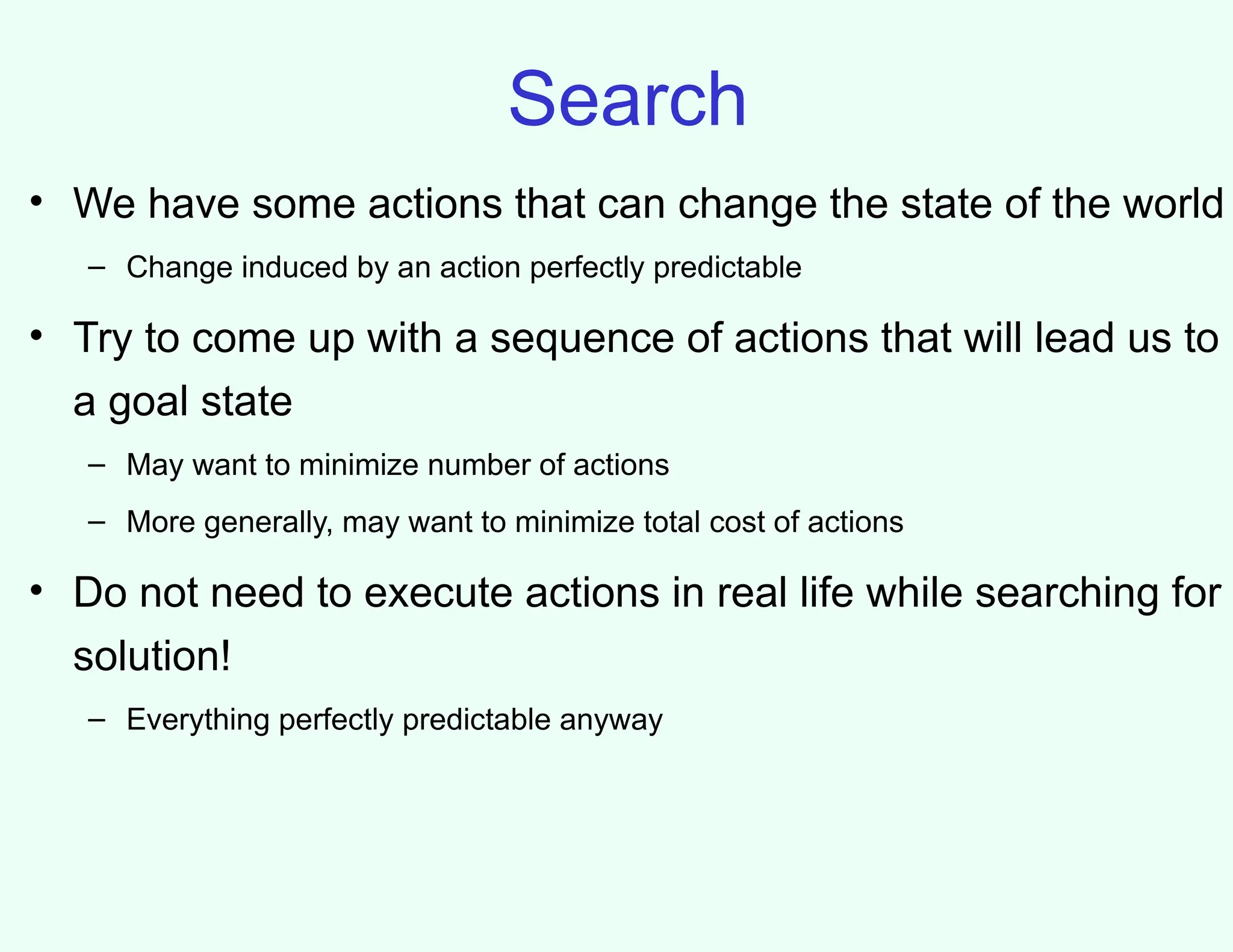
Search
• We havesome actions that can change the state of the world
– Change induced by an action perfectly predictable
• Try to come up with a sequence of actions that will lead us to
a goal state
– May want to minimize number of actions
– More generally, may want to minimize total cost of actions
• Do not need to execute actions in real life while searching for
solution!
– Everything perfectly predictable anyway
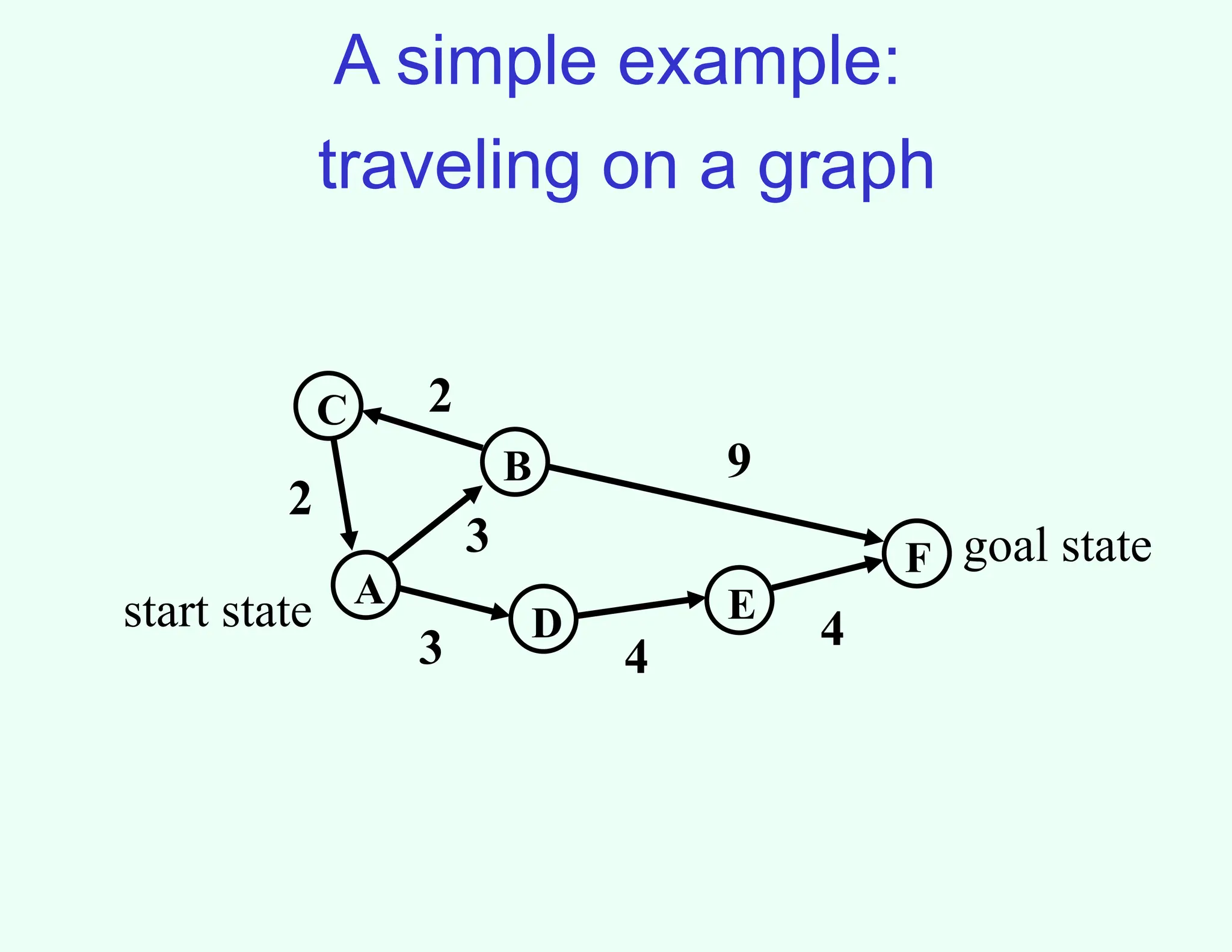
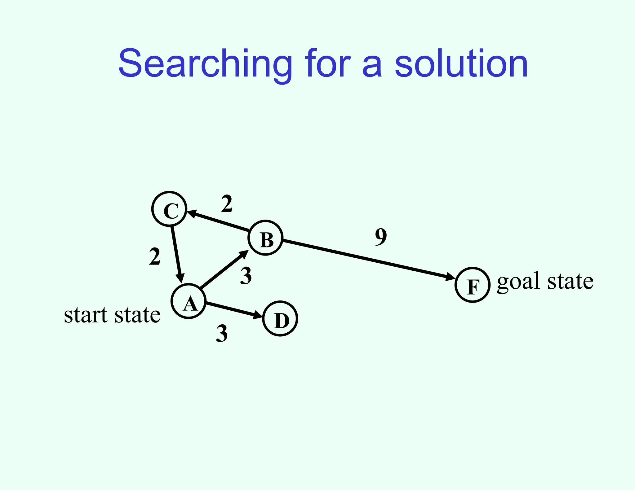
Searching for asolution
A
B
C
F
D
3
3
9
2
2
start state
goal state
5.
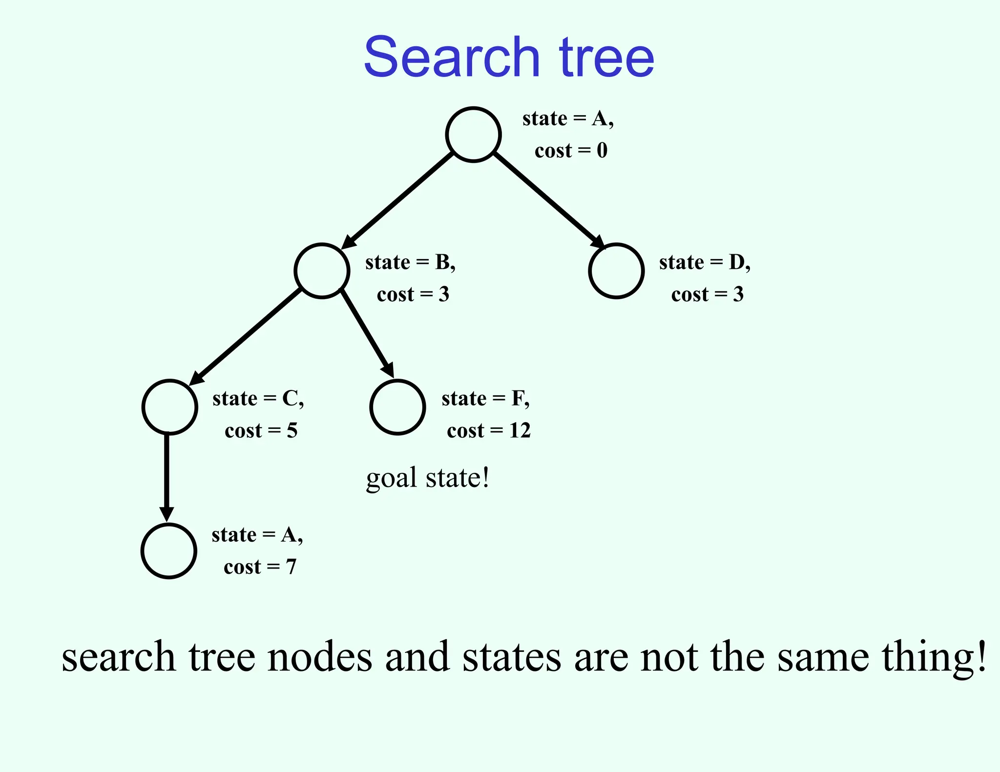
Search tree
state =A,
cost = 0
state = B,
cost = 3
state = D,
cost = 3
state = C,
cost = 5
state = F,
cost = 12
state = A,
cost = 7
goal state!
search tree nodes and states are not the same thing!
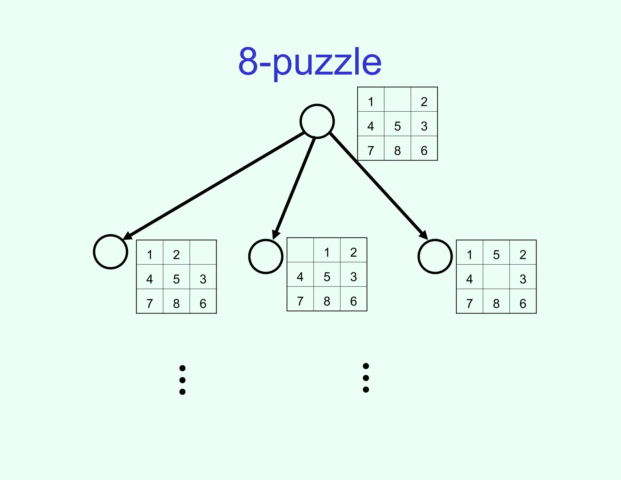
6.
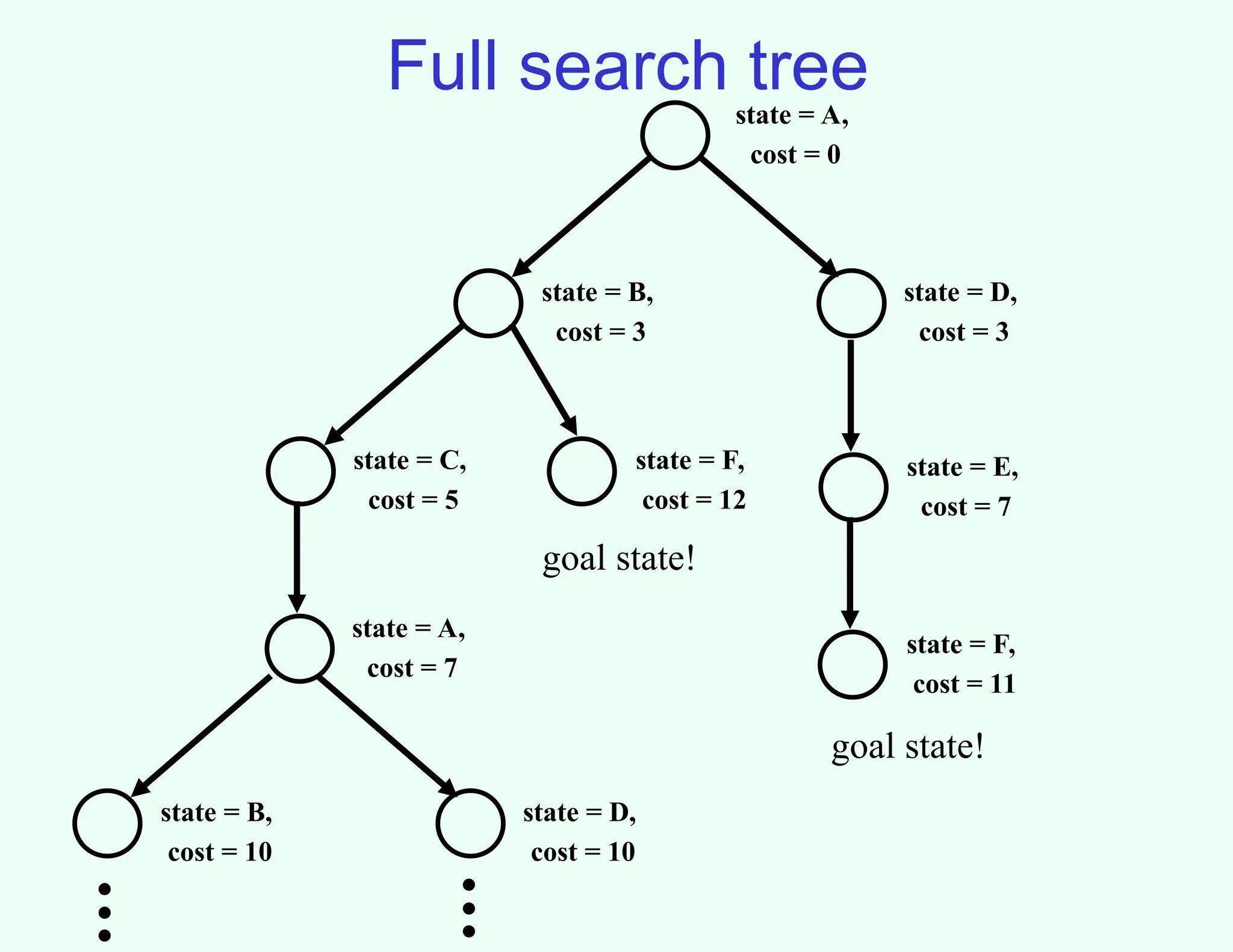
Full search tree
state= A,
cost = 0
state = B,
cost = 3
state = D,
cost = 3
state = C,
cost = 5
state = F,
cost = 12
state = A,
cost = 7
goal state!
state = E,
cost = 7
state = F,
cost = 11
goal state!
state = B,
cost = 10
state = D,
cost = 10
.
.
.
.
.
.
7.
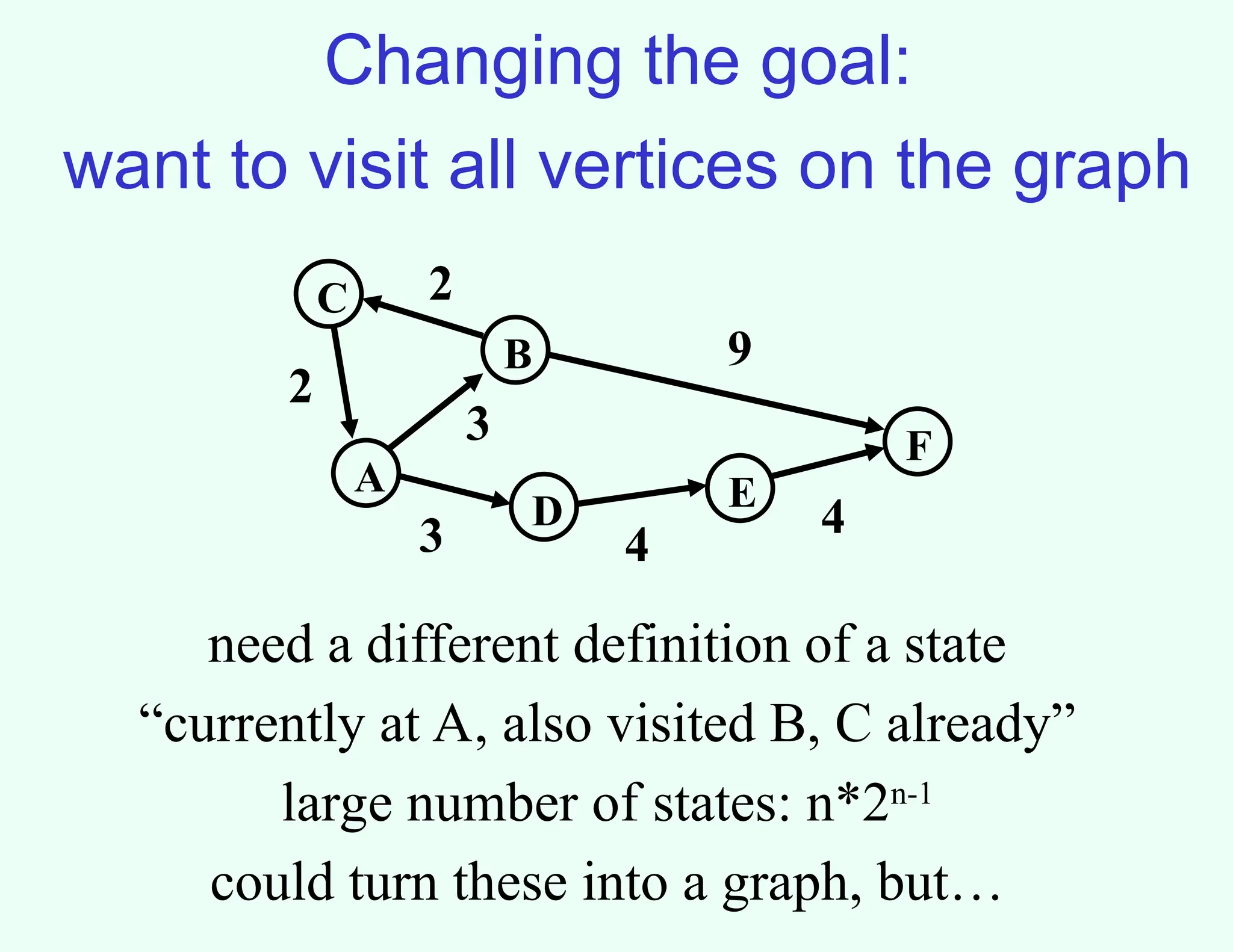
Changing the goal:
wantto visit all vertices on the graph
A
B
C
F
D E
3 4
4
3
9
2
2
need a different definition of a state
“currently at A, also visited B, C already”
large number of states: n*2n-1
could turn these into a graph, but…
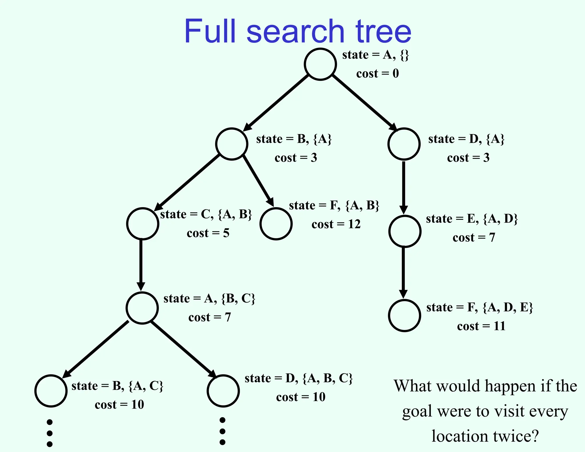
8.
Full search tree
state= A, {}
cost = 0
state = B, {A}
cost = 3
state = D, {A}
cost = 3
state = C, {A, B}
cost = 5
state = F, {A, B}
cost = 12
state = A, {B, C}
cost = 7
state = E, {A, D}
cost = 7
state = F, {A, D, E}
cost = 11
state = B, {A, C}
cost = 10
state = D, {A, B, C}
cost = 10
.
.
.
.
.
.
What would happen if the
goal were to visit every
location twice?
9.
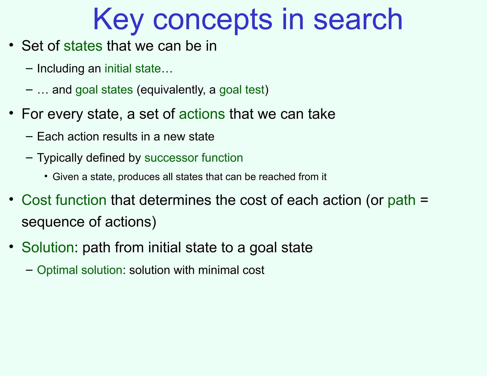
Key concepts insearch
• Set of states that we can be in
– Including an initial state…
– … and goal states (equivalently, a goal test)
• For every state, a set of actions that we can take
– Each action results in a new state
– Typically defined by successor function
• Given a state, produces all states that can be reached from it
• Cost function that determines the cost of each action (or path =
sequence of actions)
• Solution: path from initial state to a goal state
– Optimal solution: solution with minimal cost
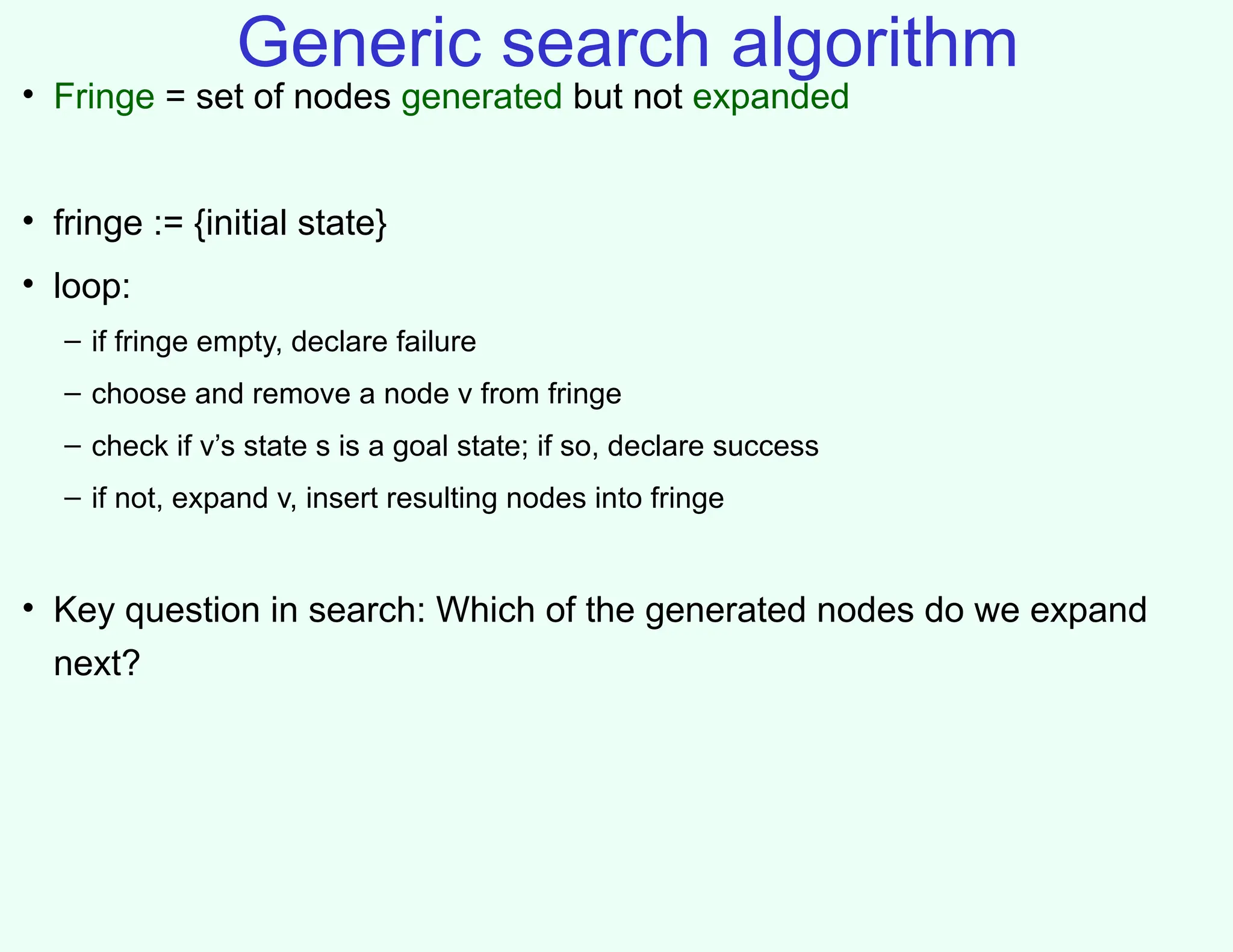
Generic search algorithm
•Fringe = set of nodes generated but not expanded
• fringe := {initial state}
• loop:
– if fringe empty, declare failure
– choose and remove a node v from fringe
– check if v’s state s is a goal state; if so, declare success
– if not, expand v, insert resulting nodes into fringe
• Key question in search: Which of the generated nodes do we expand
next?
13.
Uninformed search
• Givena state, we only know whether it is a goal
state or not
• Cannot say one nongoal state looks better than
another nongoal state
• Can only traverse state space blindly in hope of
somehow hitting a goal state at some point
– Also called blind search
– Blind does not imply unsystematic!
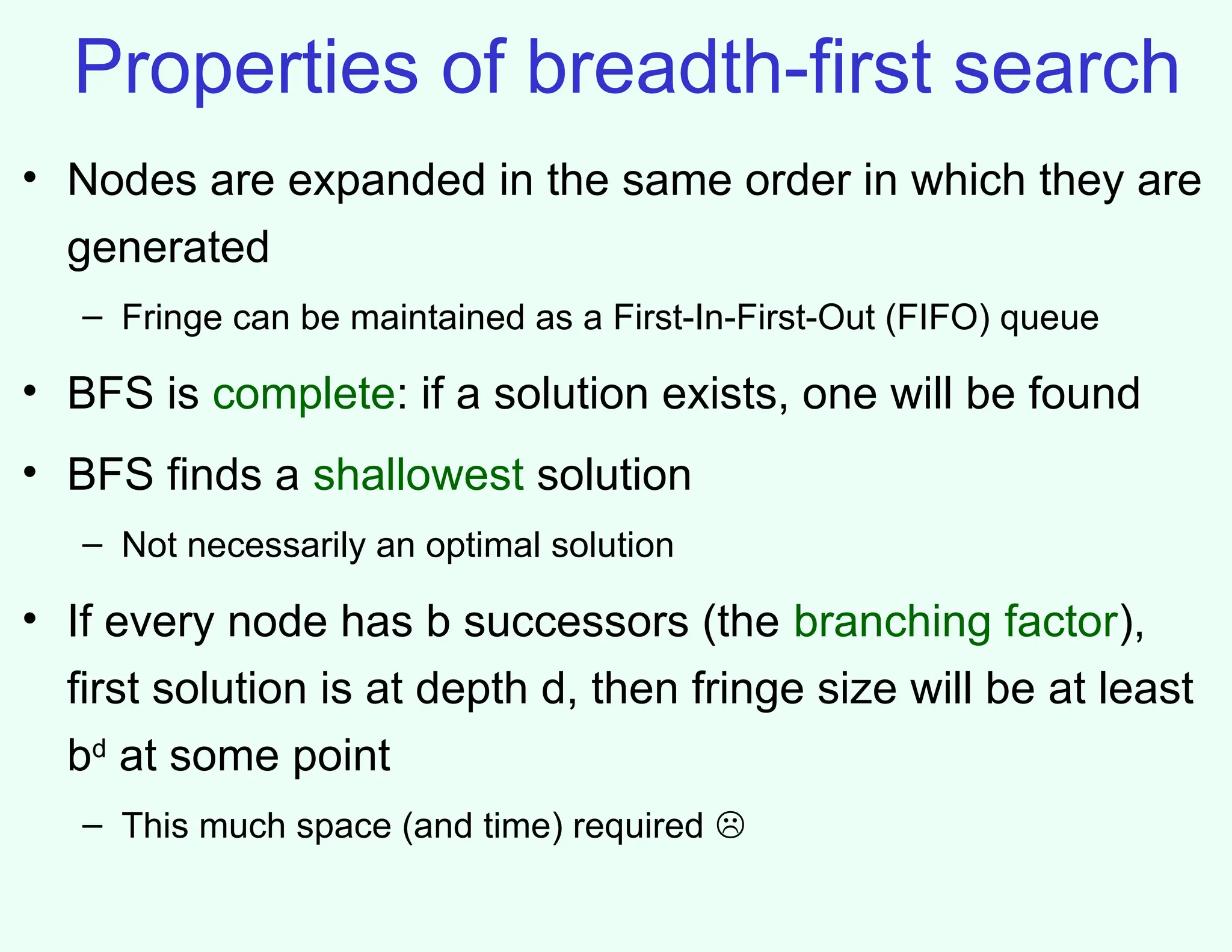
Properties of breadth-firstsearch
• Nodes are expanded in the same order in which they are
generated
– Fringe can be maintained as a First-In-First-Out (FIFO) queue
• BFS is complete: if a solution exists, one will be found
• BFS finds a shallowest solution
– Not necessarily an optimal solution
• If every node has b successors (the branching factor),
first solution is at depth d, then fringe size will be at least
bd
at some point
– This much space (and time) required
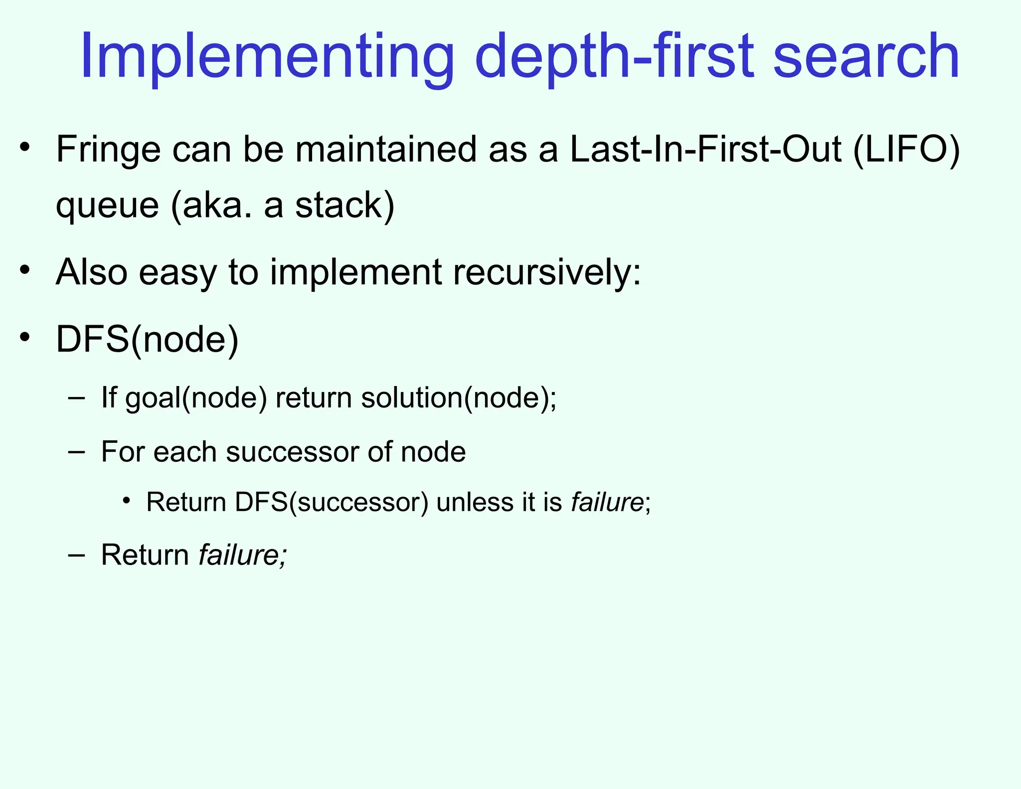
Implementing depth-first search
•Fringe can be maintained as a Last-In-First-Out (LIFO)
queue (aka. a stack)
• Also easy to implement recursively:
• DFS(node)
– If goal(node) return solution(node);
– For each successor of node
• Return DFS(successor) unless it is failure;
– Return failure;
18.
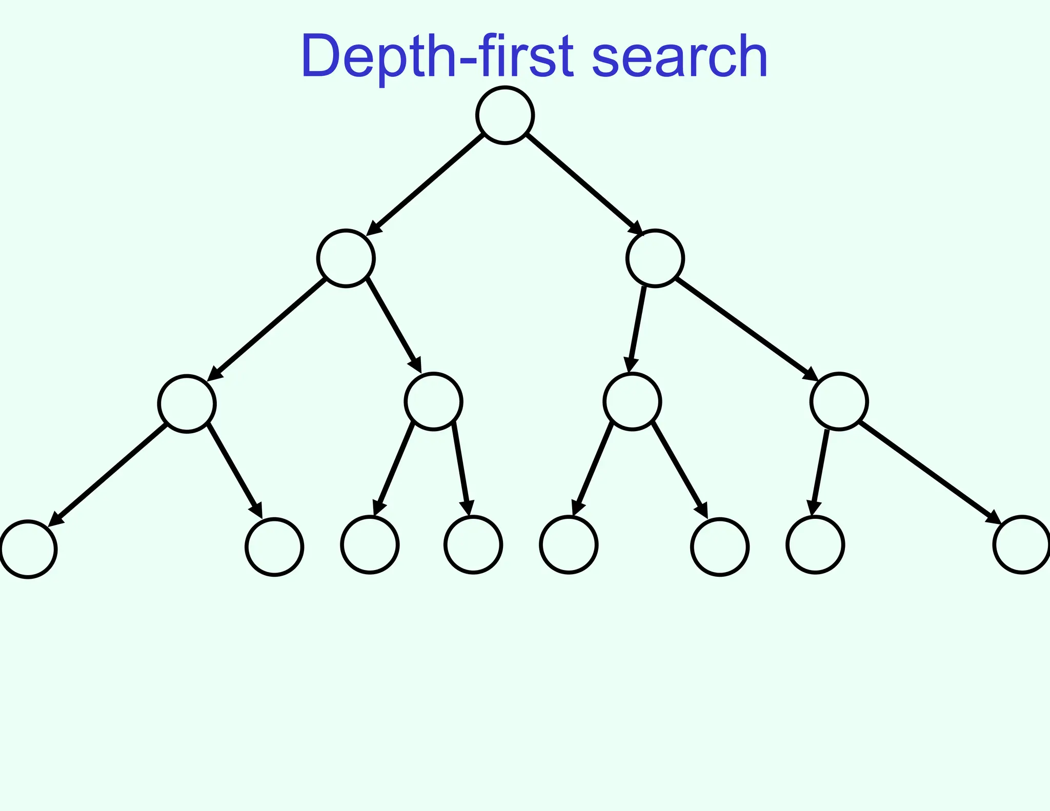
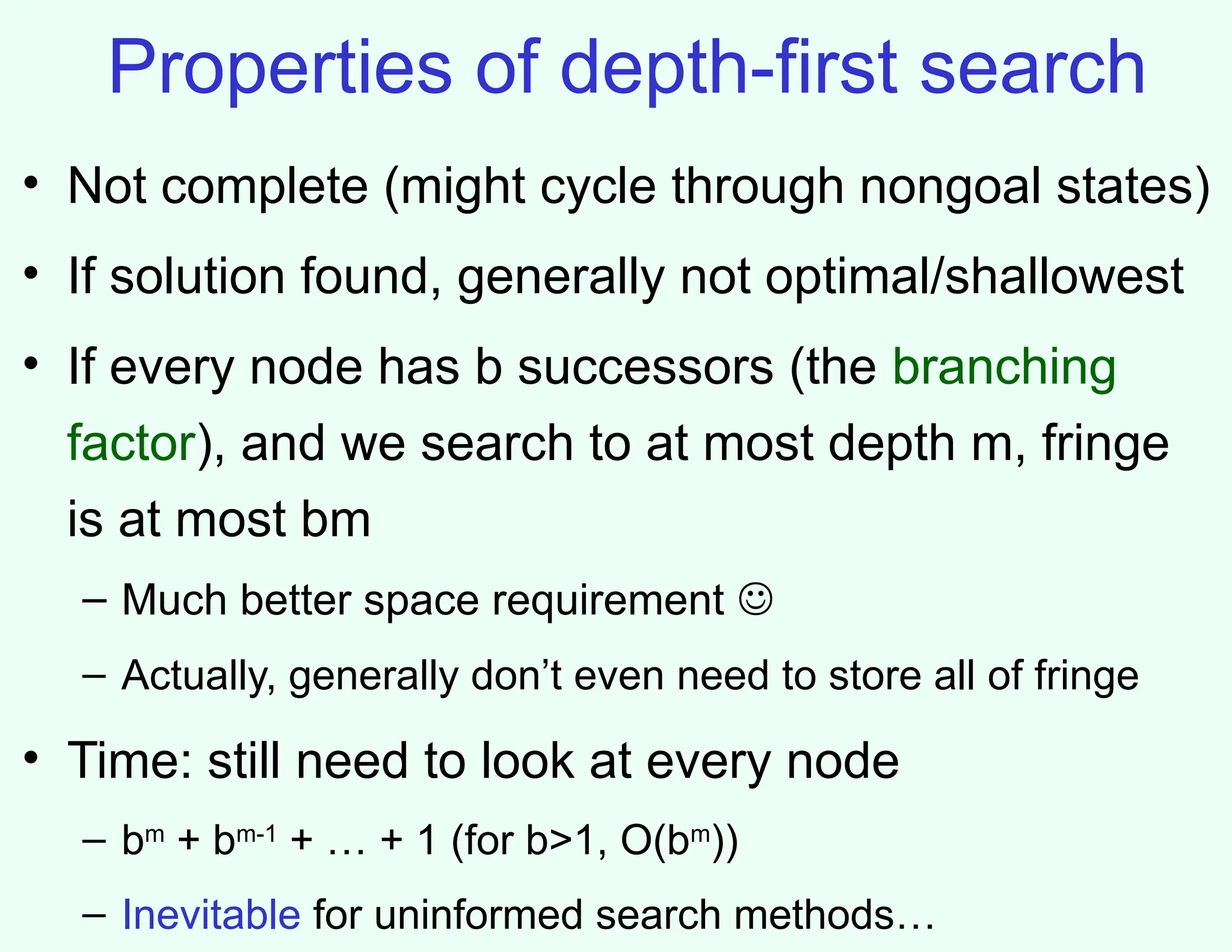
Properties of depth-firstsearch
• Not complete (might cycle through nongoal states)
• If solution found, generally not optimal/shallowest
• If every node has b successors (the branching
factor), and we search to at most depth m, fringe
is at most bm
– Much better space requirement
– Actually, generally don’t even need to store all of fringe
• Time: still need to look at every node
– bm
+ bm-1
+ … + 1 (for b>1, O(bm
))
– Inevitable for uninformed search methods…
19.
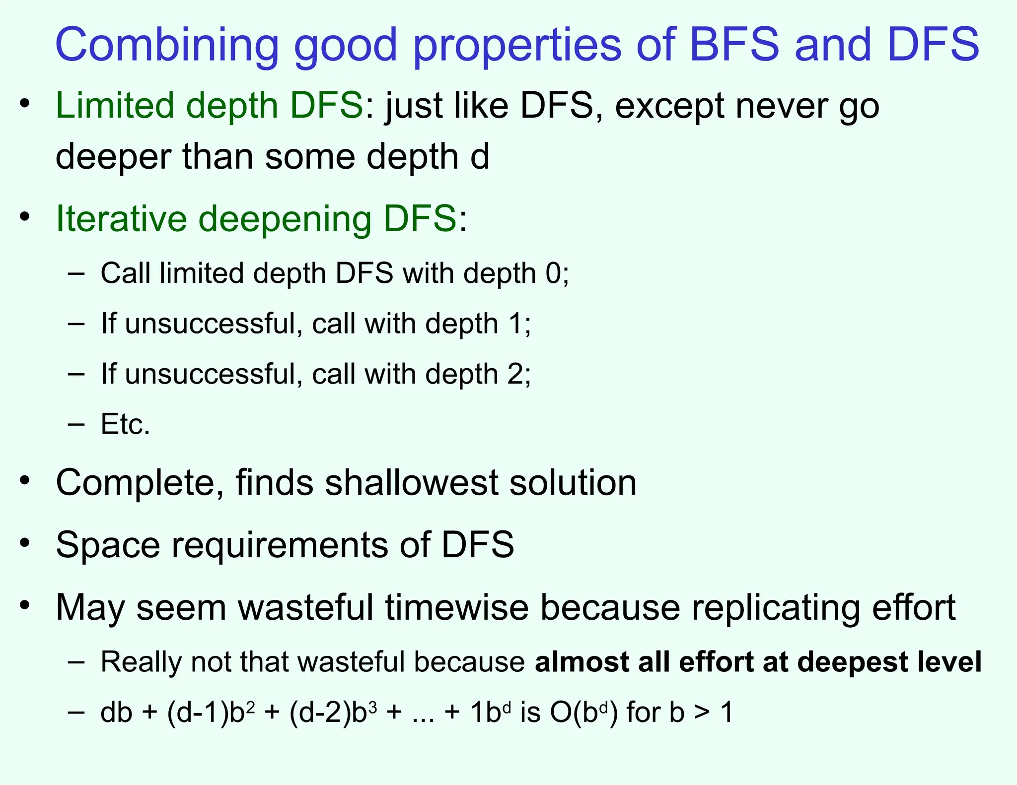
Combining good propertiesof BFS and DFS
• Limited depth DFS: just like DFS, except never go
deeper than some depth d
• Iterative deepening DFS:
– Call limited depth DFS with depth 0;
– If unsuccessful, call with depth 1;
– If unsuccessful, call with depth 2;
– Etc.
• Complete, finds shallowest solution
• Space requirements of DFS
• May seem wasteful timewise because replicating effort
– Really not that wasteful because almost all effort at deepest level
– db + (d-1)b2
+ (d-2)b3
+ ... + 1bd
is O(bd
) for b > 1
20.
Let’s start thinkingabout cost
• BFS finds shallowest solution because always works on
shallowest nodes first
• Similar idea: always work on the lowest-cost node first
(uniform-cost search)
• Will find optimal solution (assuming costs increase by at
least constant amount along path)
• Will often pursue lots of short steps first
• If optimal cost is C, and cost increases by at least L each
step, we can go to depth C/L
• Similar memory problems as BFS
– Iterative lengthening DFS does DFS up to increasing costs
21.
Searching backwards fromthe goal
• Sometimes can search backwards from the goal
– Maze puzzles
– Eights puzzle
– Reaching location F
– What about the goal of “having visited all locations”?
• Need to be able to compute predecessors instead
of successors
• What’s the point?
22.
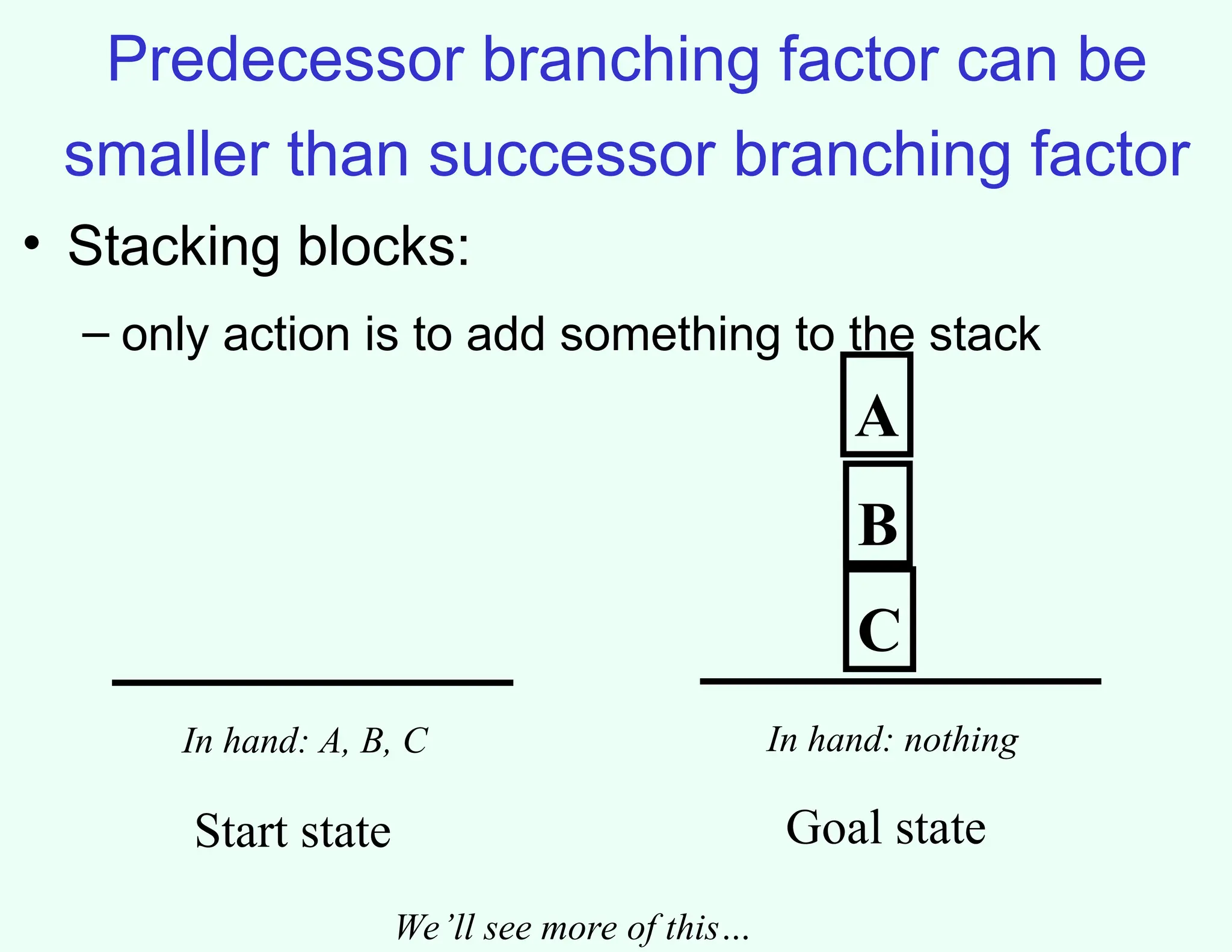
Predecessor branching factorcan be
smaller than successor branching factor
• Stacking blocks:
– only action is to add something to the stack
A
B
C
In hand: nothing
In hand: A, B, C
Start state Goal state
We’ll see more of this…
23.
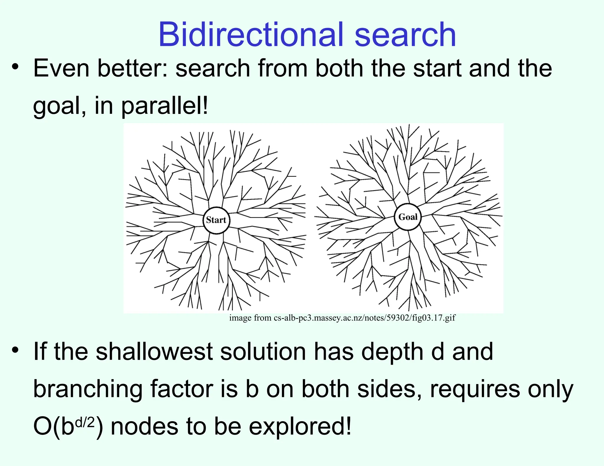
Bidirectional search
• Evenbetter: search from both the start and the
goal, in parallel!
• If the shallowest solution has depth d and
branching factor is b on both sides, requires only
O(bd/2
) nodes to be explored!
image from cs-alb-pc3.massey.ac.nz/notes/59302/fig03.17.gif
24.
Making bidirectional searchwork
• Need to be able to figure out whether the fringes
intersect
– Need to keep at least one fringe in memory…
• Other than that, can do various kinds of search on
either tree, and get the corresponding optimality
etc. guarantees
• Not possible (feasible) if backwards search not
possible (feasible)
– Hard to compute predecessors
– High predecessor branching factor
– Too many goal states
25.
Repeated states
• Repeatedstates can cause incompleteness or enormous
runtimes
• Can maintain list of previously visited states to avoid this
– If new path to the same state has greater cost, don’t pursue it further
– Leads to time/space tradeoff
• “Algorithms that forget their history are doomed to repeat
it” [Russell and Norvig]
A
B
C
3
2
2
cycles exponentially large search trees (try it!)
26.
Informed search
• Sofar, have assumed that no nongoal state looks
better than another
• Unrealistic
– Even without knowing the road structure, some locations
seem closer to the goal than others
– Some states of the 8s puzzle seem closer to the goal than
others
• Makes sense to expand closer-seeming nodes
first
27.
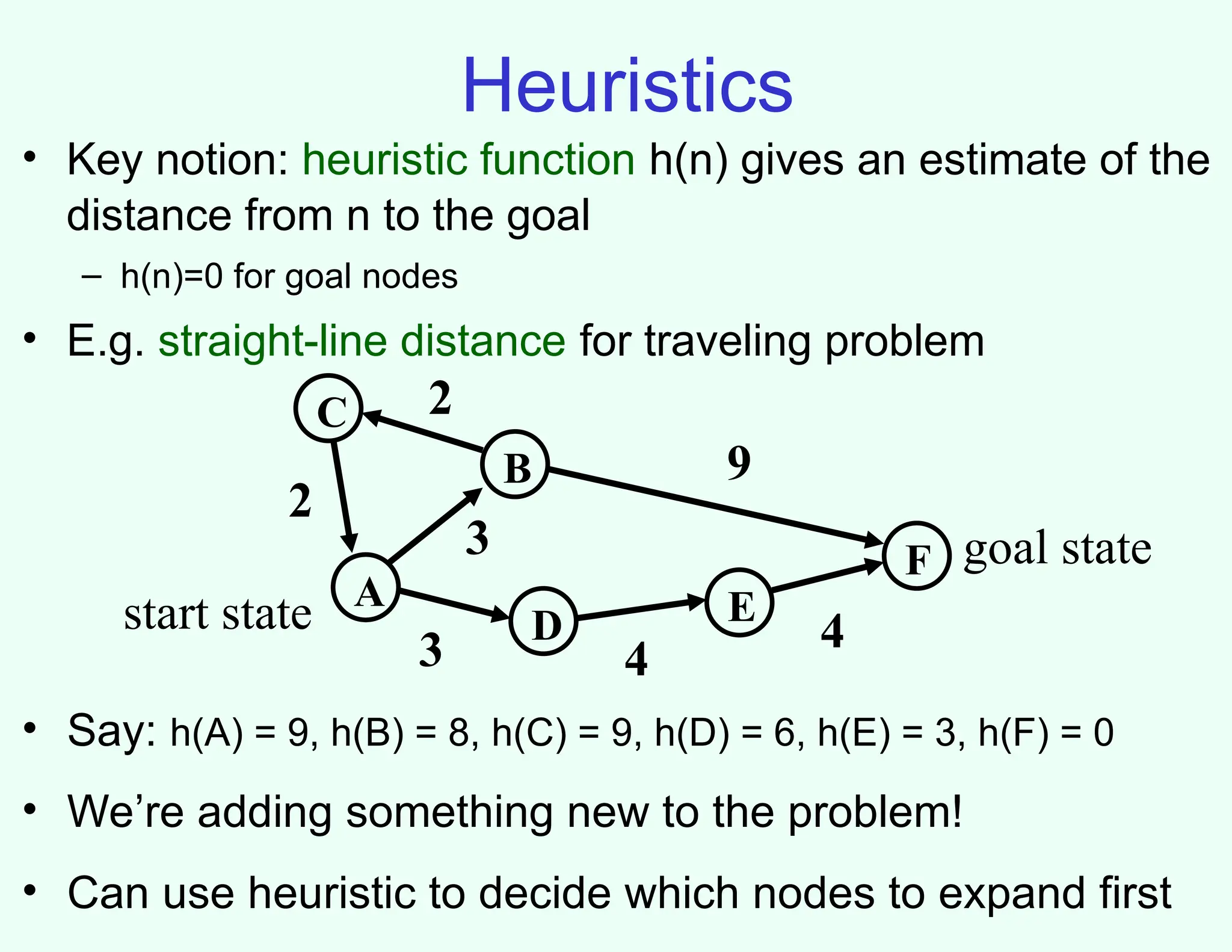
Heuristics
• Key notion:heuristic function h(n) gives an estimate of the
distance from n to the goal
– h(n)=0 for goal nodes
• E.g. straight-line distance for traveling problem
A
B
C
F
D E
3 4
4
3
9
2
2
start state
goal state
• Say: h(A) = 9, h(B) = 8, h(C) = 9, h(D) = 6, h(E) = 3, h(F) = 0
• We’re adding something new to the problem!
• Can use heuristic to decide which nodes to expand first
28.
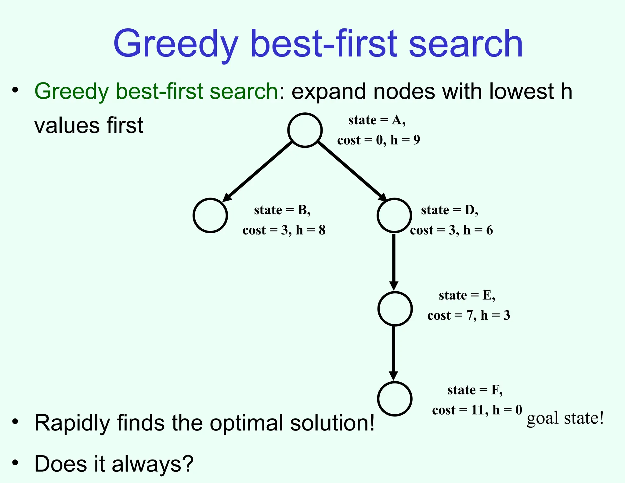
Greedy best-first search
•Greedy best-first search: expand nodes with lowest h
values first
• Rapidly finds the optimal solution!
• Does it always?
state = A,
cost = 0, h = 9
state = B,
cost = 3, h = 8
state = D,
cost = 3, h = 6
goal state!
state = E,
cost = 7, h = 3
state = F,
cost = 11, h = 0
29.
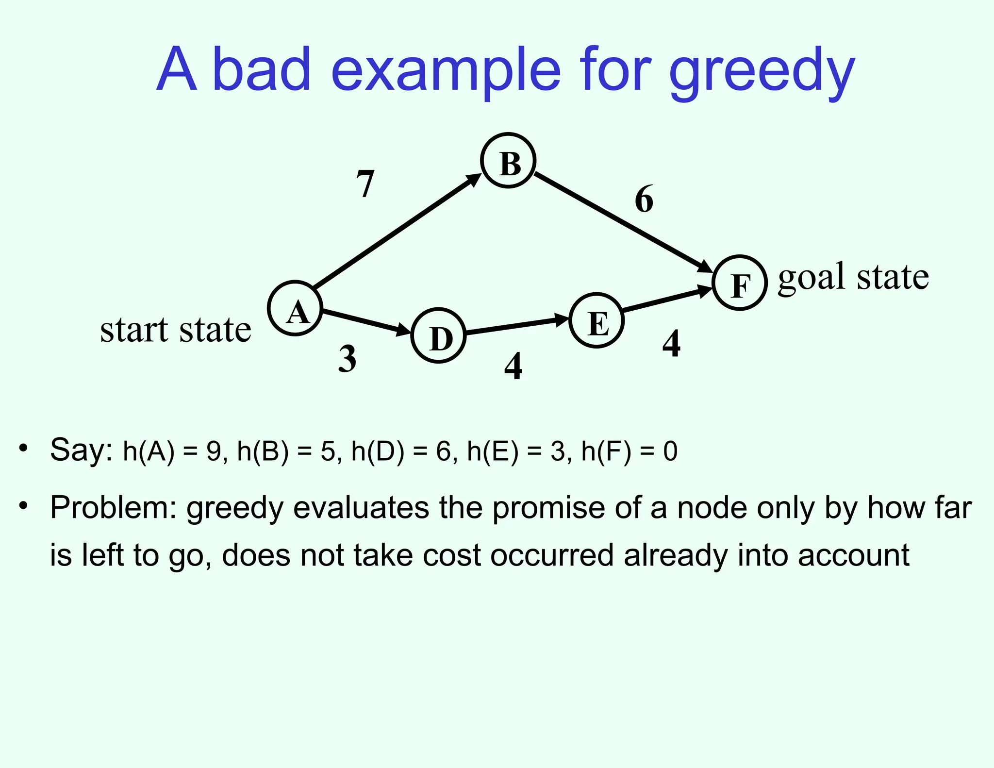
A bad examplefor greedy
A
B
F
D E
3 4
4
7 6
start state
goal state
• Say: h(A) = 9, h(B) = 5, h(D) = 6, h(E) = 3, h(F) = 0
• Problem: greedy evaluates the promise of a node only by how far
is left to go, does not take cost occurred already into account
30.
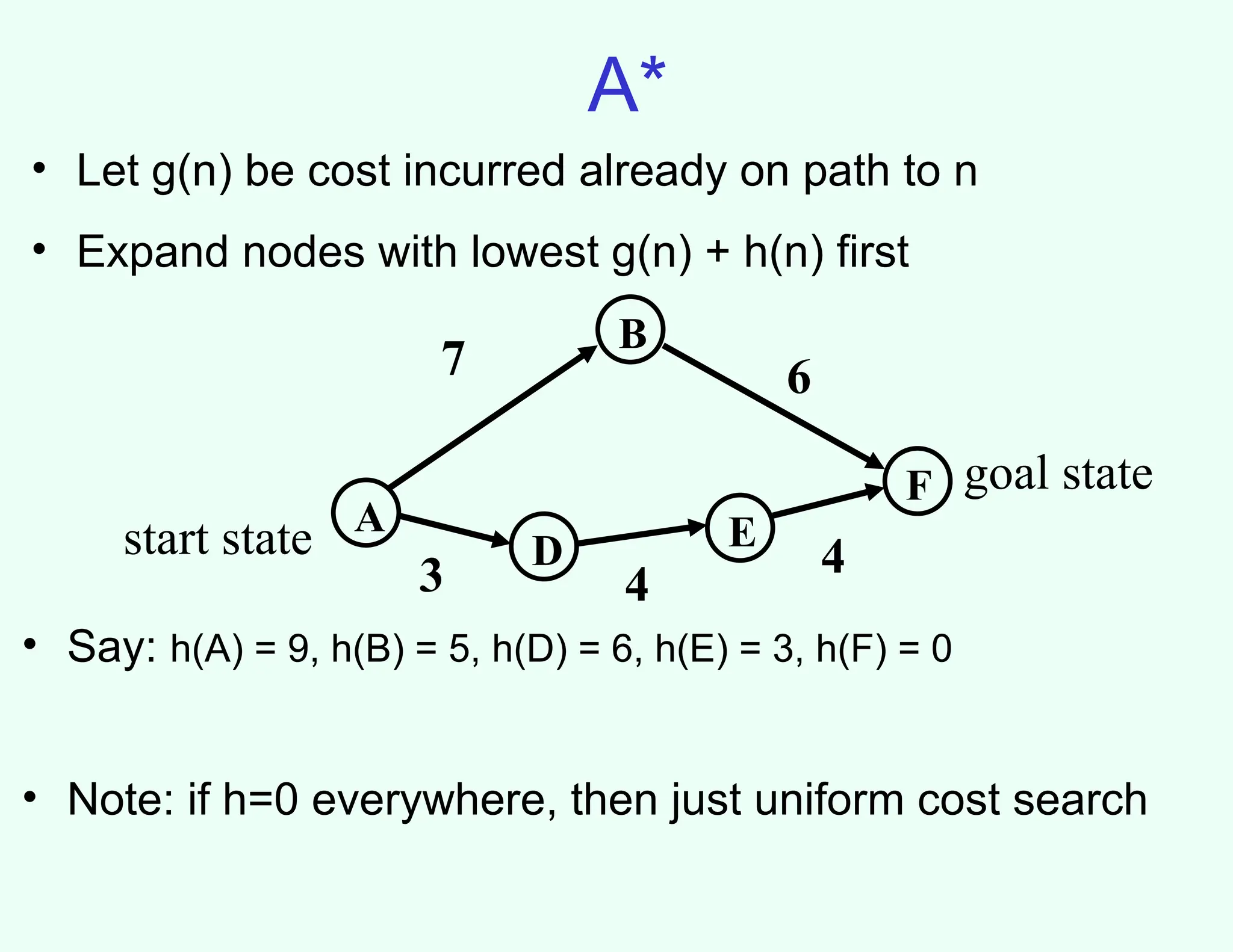
A*
A
B
F
D E
3 4
4
76
start state
goal state
• Say: h(A) = 9, h(B) = 5, h(D) = 6, h(E) = 3, h(F) = 0
• Note: if h=0 everywhere, then just uniform cost search
• Let g(n) be cost incurred already on path to n
• Expand nodes with lowest g(n) + h(n) first
31.
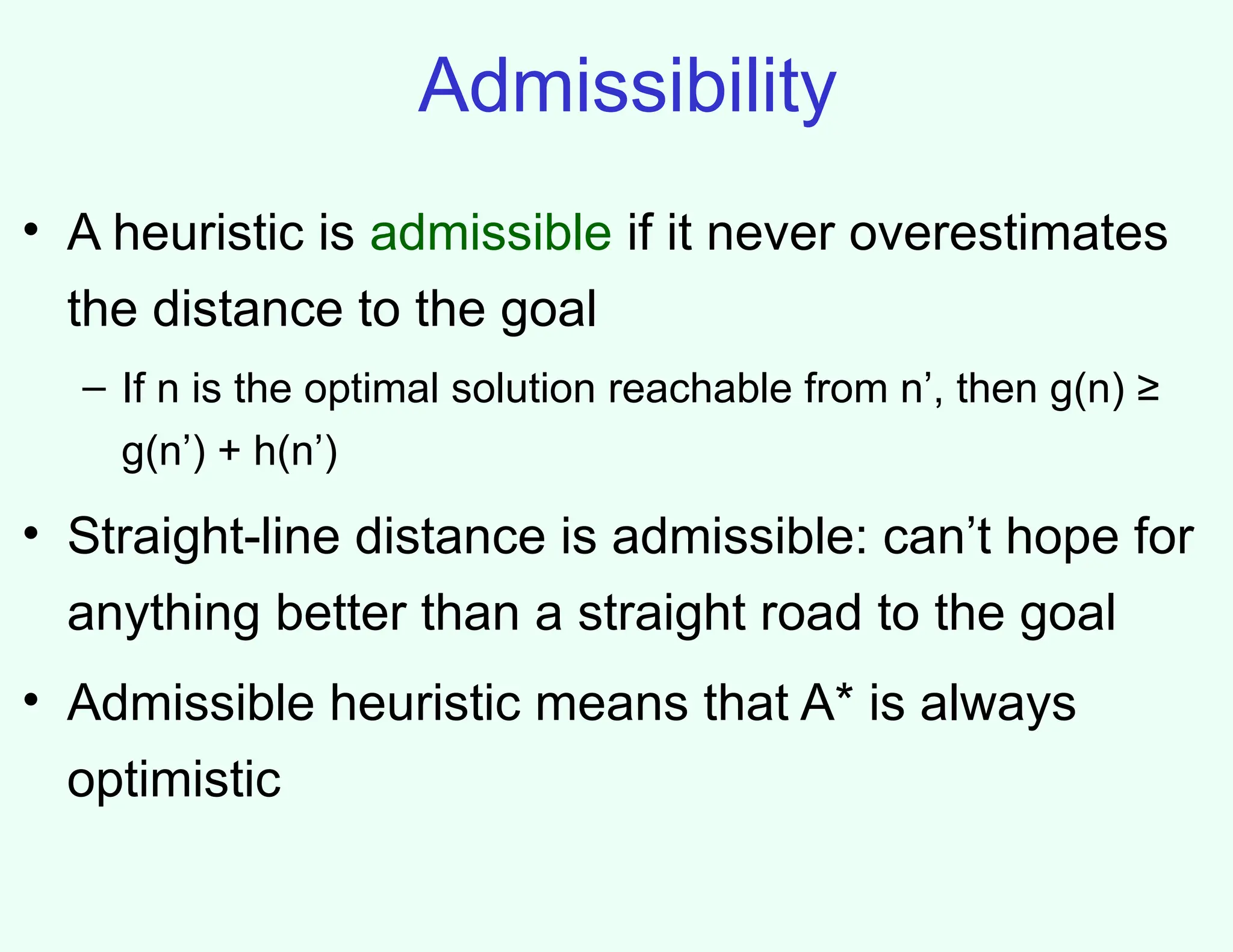
Admissibility
• A heuristicis admissible if it never overestimates
the distance to the goal
– If n is the optimal solution reachable from n’, then g(n) ≥
g(n’) + h(n’)
• Straight-line distance is admissible: can’t hope for
anything better than a straight road to the goal
• Admissible heuristic means that A* is always
optimistic
32.
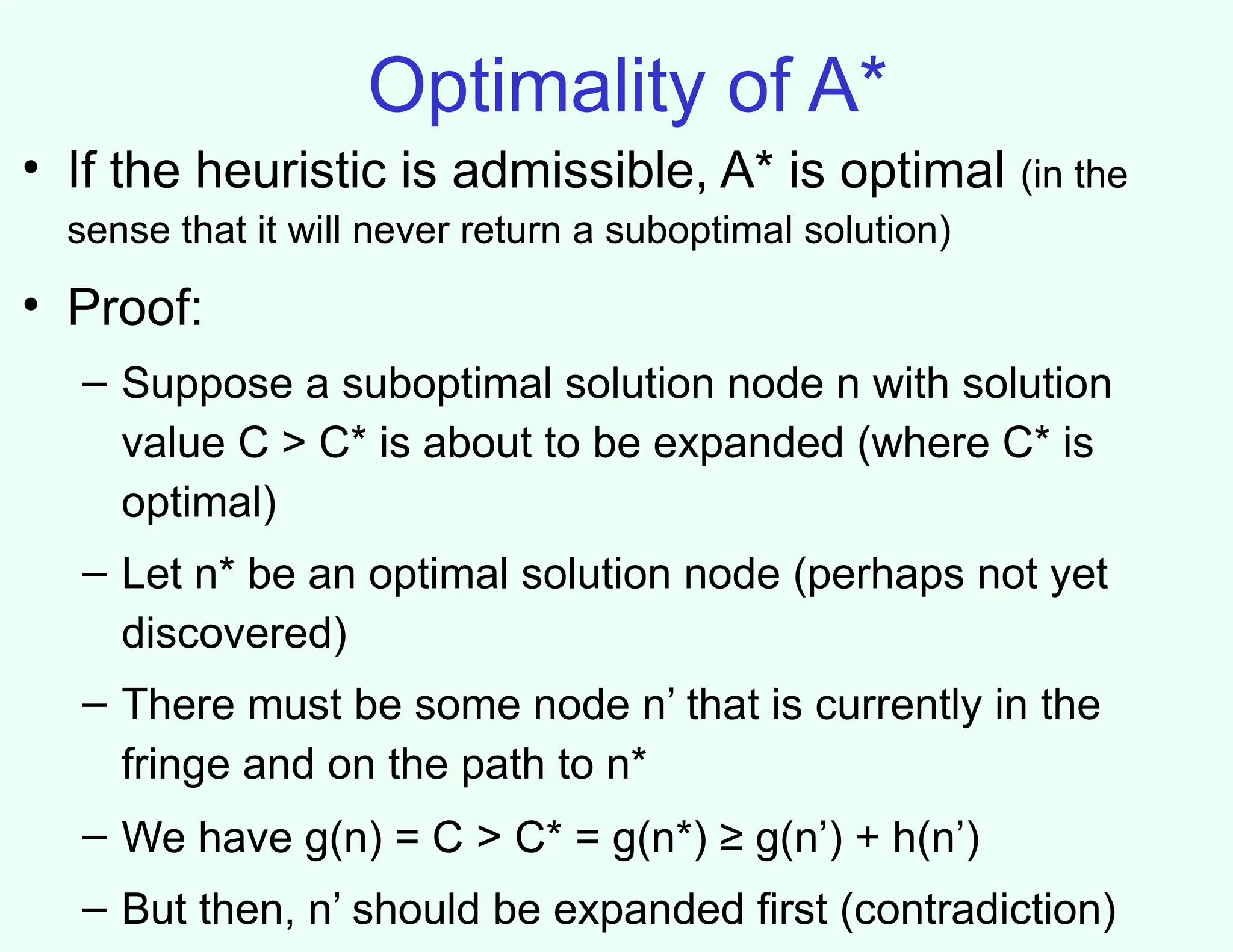
Optimality of A*
•If the heuristic is admissible, A* is optimal (in the
sense that it will never return a suboptimal solution)
• Proof:
– Suppose a suboptimal solution node n with solution
value C > C* is about to be expanded (where C* is
optimal)
– Let n* be an optimal solution node (perhaps not yet
discovered)
– There must be some node n’ that is currently in the
fringe and on the path to n*
– We have g(n) = C > C* = g(n*) ≥ g(n’) + h(n’)
– But then, n’ should be expanded first (contradiction)
33.
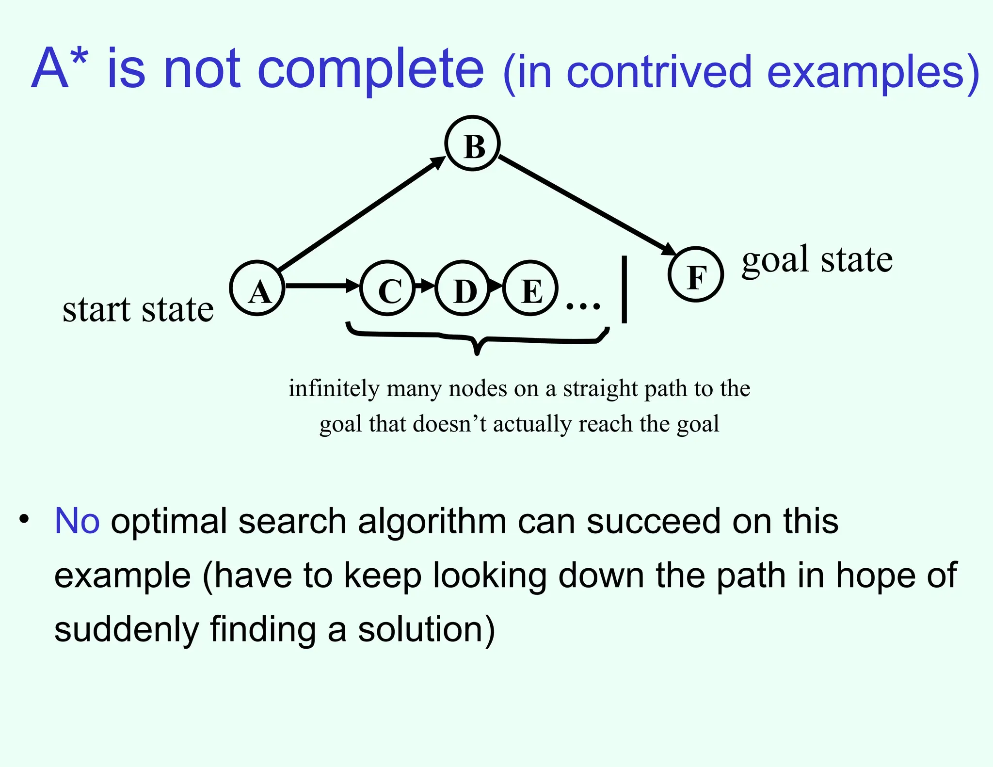
A* is notcomplete (in contrived examples)
A
B
F
D …
start state
goal state
• No optimal search algorithm can succeed on this
example (have to keep looking down the path in hope of
suddenly finding a solution)
C E
infinitely many nodes on a straight path to the
goal that doesn’t actually reach the goal
34.
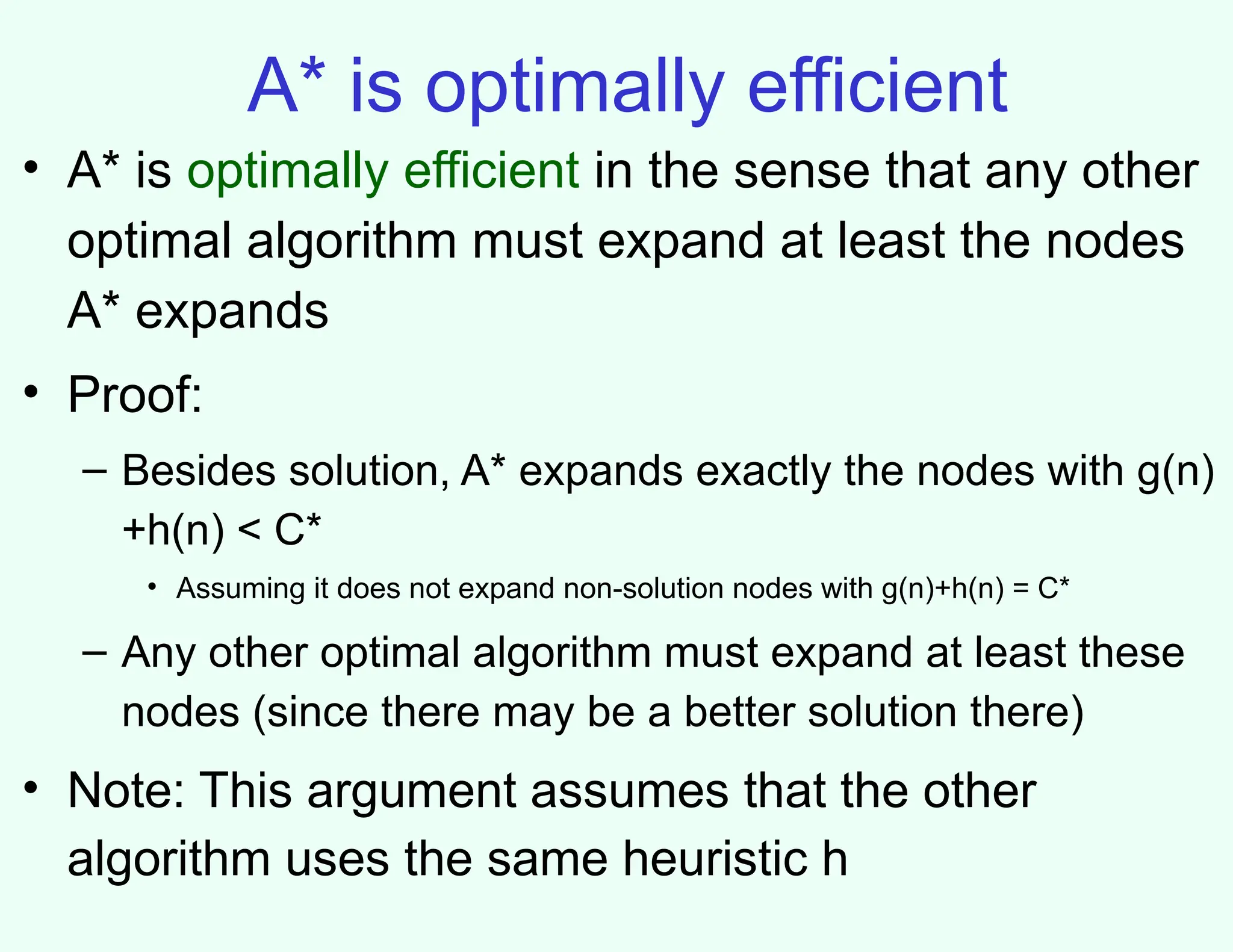
A* is optimallyefficient
• A* is optimally efficient in the sense that any other
optimal algorithm must expand at least the nodes
A* expands
• Proof:
– Besides solution, A* expands exactly the nodes with g(n)
+h(n) < C*
• Assuming it does not expand non-solution nodes with g(n)+h(n) = C*
– Any other optimal algorithm must expand at least these
nodes (since there may be a better solution there)
• Note: This argument assumes that the other
algorithm uses the same heuristic h
35.
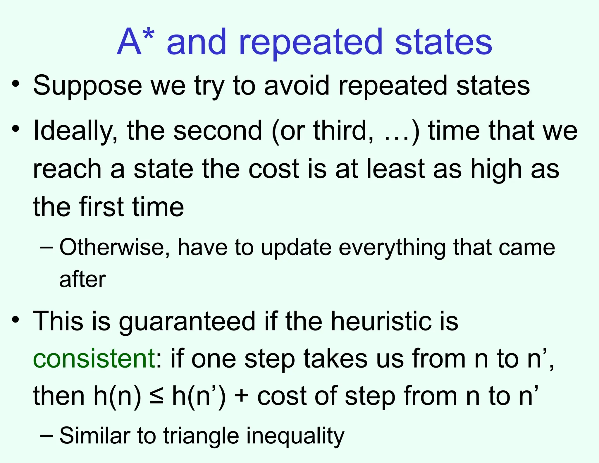
A* and repeatedstates
• Suppose we try to avoid repeated states
• Ideally, the second (or third, …) time that we
reach a state the cost is at least as high as
the first time
– Otherwise, have to update everything that came
after
• This is guaranteed if the heuristic is
consistent: if one step takes us from n to n’,
then h(n) ≤ h(n’) + cost of step from n to n’
– Similar to triangle inequality
36.
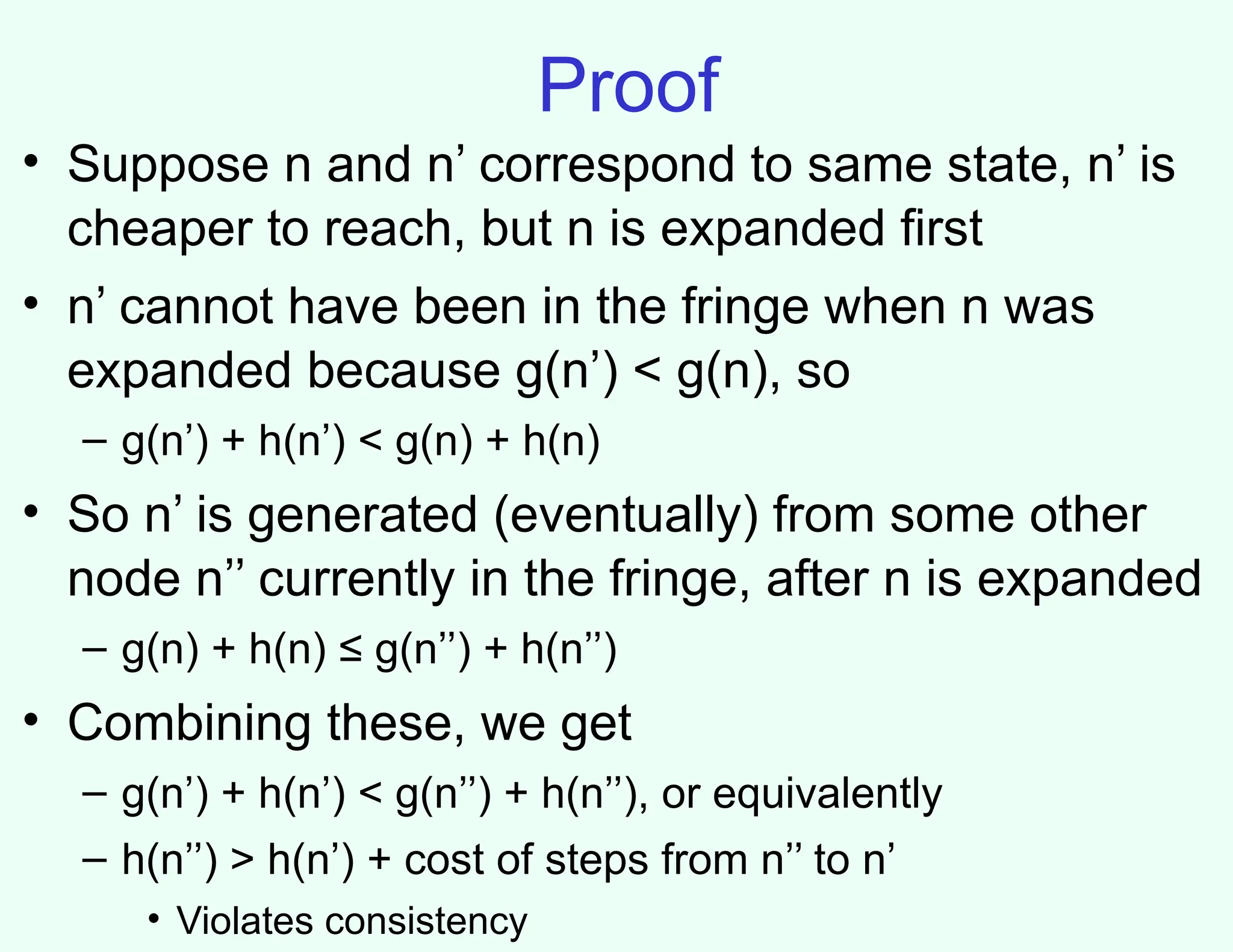
Proof
• Suppose nand n’ correspond to same state, n’ is
cheaper to reach, but n is expanded first
• n’ cannot have been in the fringe when n was
expanded because g(n’) < g(n), so
– g(n’) + h(n’) < g(n) + h(n)
• So n’ is generated (eventually) from some other
node n’’ currently in the fringe, after n is expanded
– g(n) + h(n) ≤ g(n’’) + h(n’’)
• Combining these, we get
– g(n’) + h(n’) < g(n’’) + h(n’’), or equivalently
– h(n’’) > h(n’) + cost of steps from n’’ to n’
• Violates consistency
37.
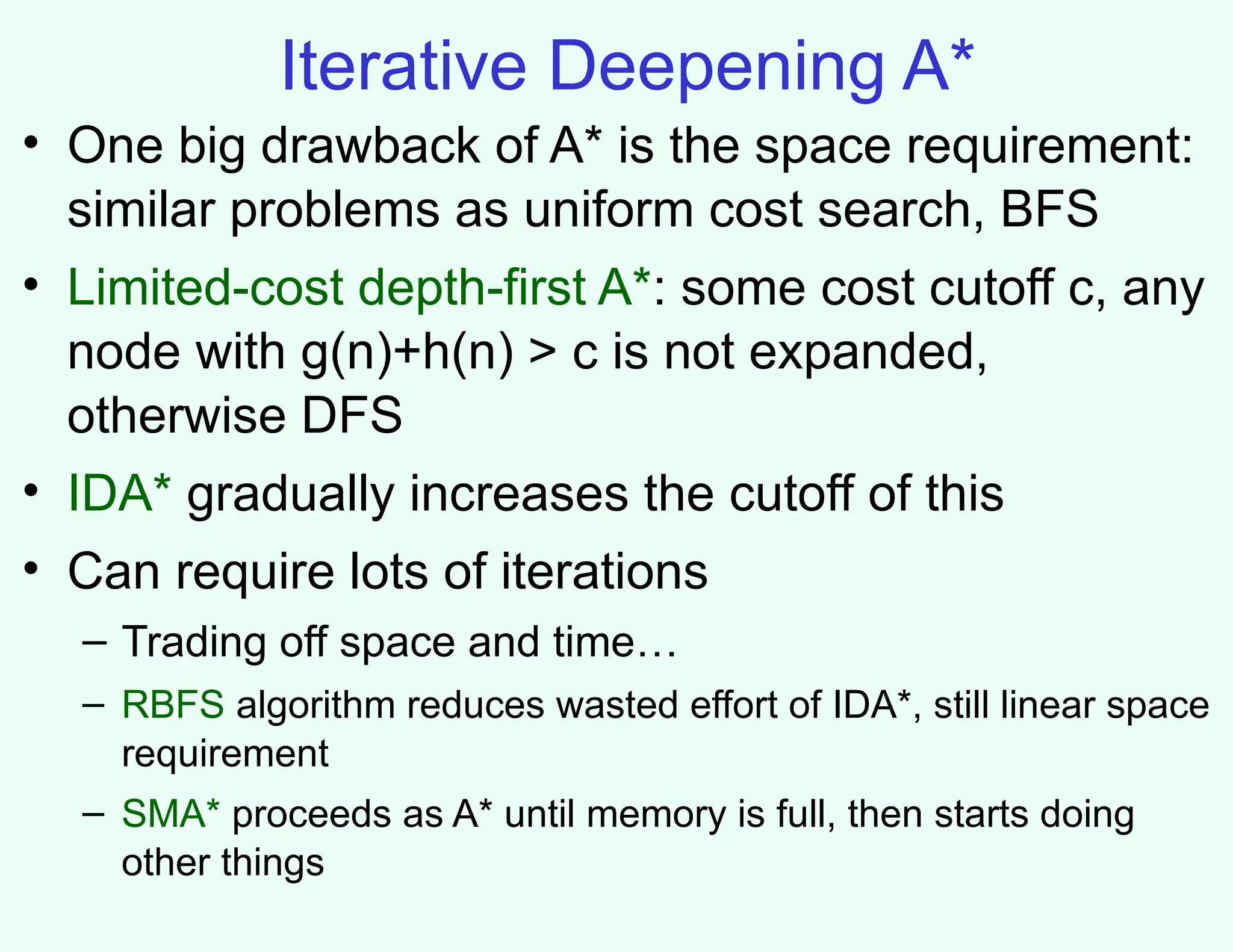
Iterative Deepening A*
•One big drawback of A* is the space requirement:
similar problems as uniform cost search, BFS
• Limited-cost depth-first A*: some cost cutoff c, any
node with g(n)+h(n) > c is not expanded,
otherwise DFS
• IDA* gradually increases the cutoff of this
• Can require lots of iterations
– Trading off space and time…
– RBFS algorithm reduces wasted effort of IDA*, still linear space
requirement
– SMA* proceeds as A* until memory is full, then starts doing
other things
38.
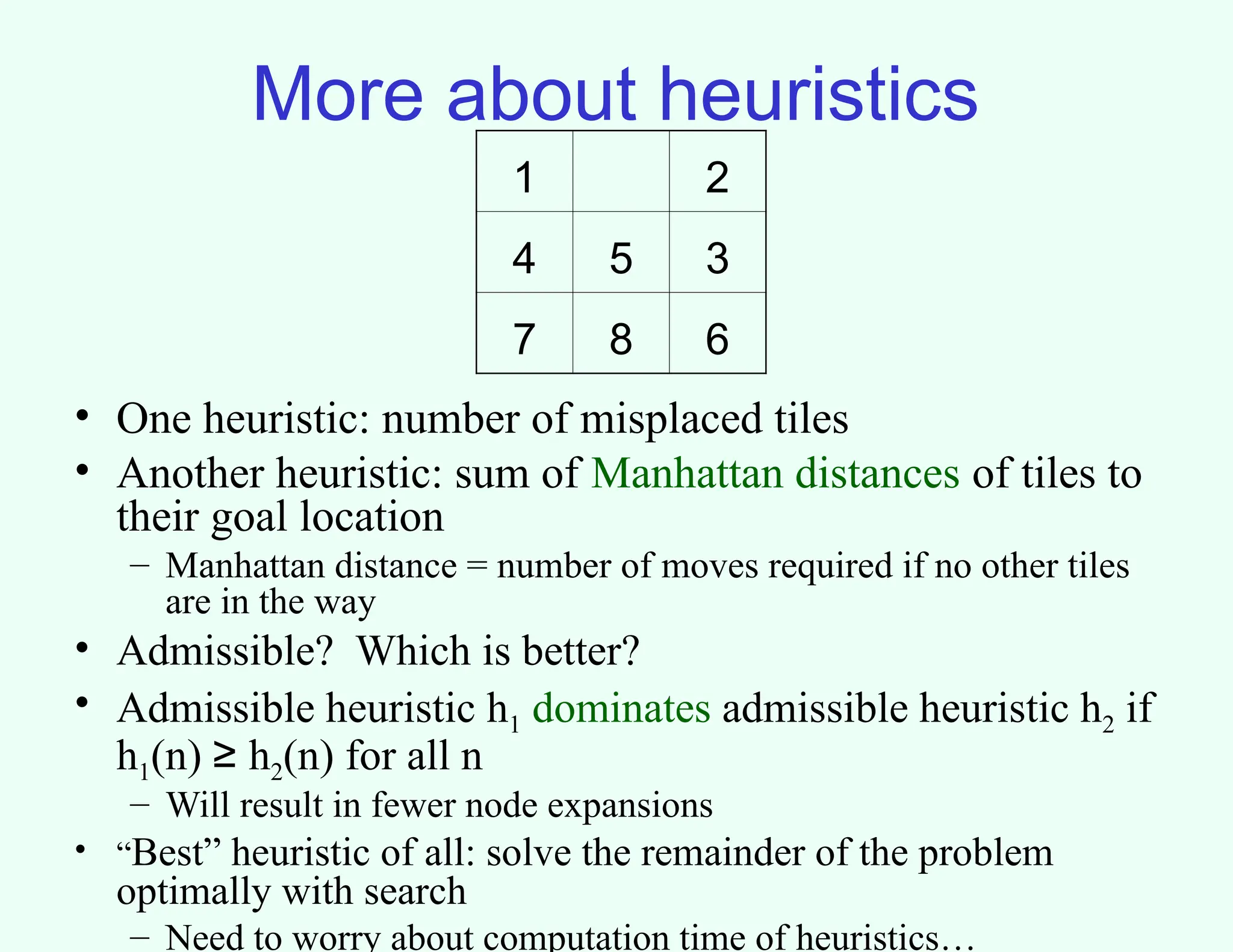
More about heuristics
•One heuristic: number of misplaced tiles
• Another heuristic: sum of Manhattan distances of tiles to
their goal location
– Manhattan distance = number of moves required if no other tiles
are in the way
• Admissible? Which is better?
• Admissible heuristic h1 dominates admissible heuristic h2 if
h1(n) ≥ h2(n) for all n
– Will result in fewer node expansions
• “Best” heuristic of all: solve the remainder of the problem
optimally with search
– Need to worry about computation time of heuristics…
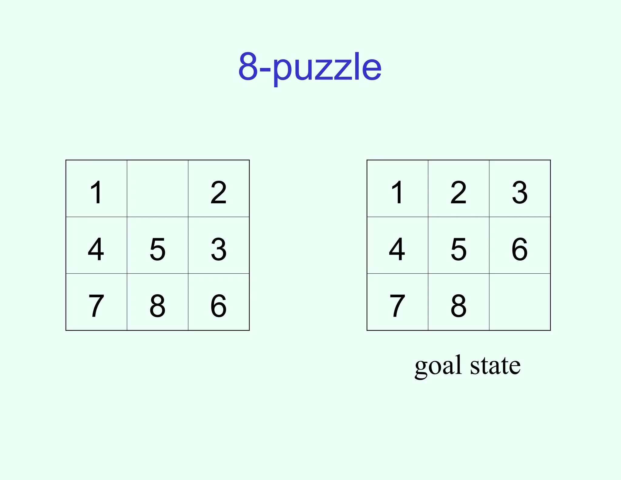
1 2
4 5 3
7 8 6
39.
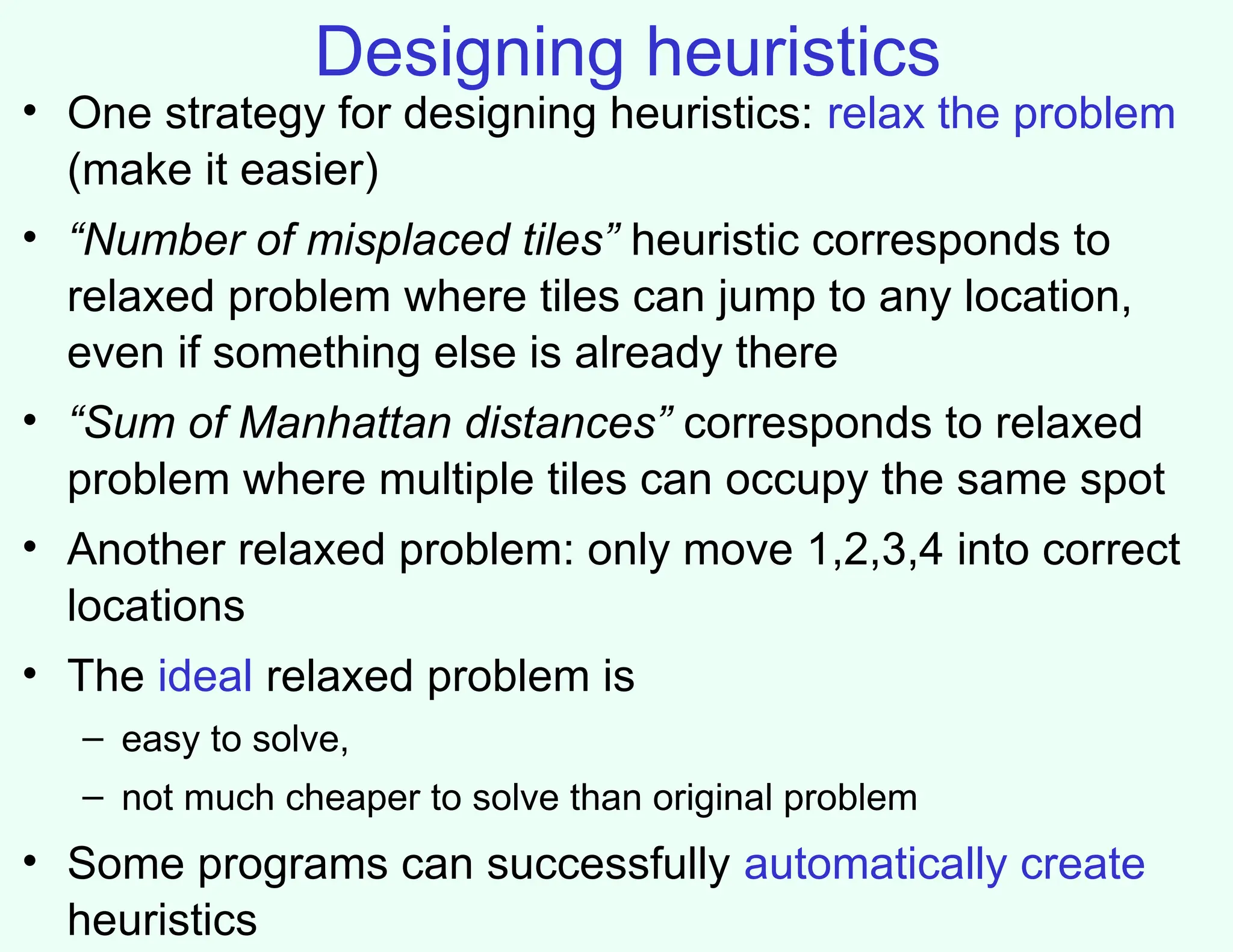
Designing heuristics
• Onestrategy for designing heuristics: relax the problem
(make it easier)
• “Number of misplaced tiles” heuristic corresponds to
relaxed problem where tiles can jump to any location,
even if something else is already there
• “Sum of Manhattan distances” corresponds to relaxed
problem where multiple tiles can occupy the same spot
• Another relaxed problem: only move 1,2,3,4 into correct
locations
• The ideal relaxed problem is
– easy to solve,
– not much cheaper to solve than original problem
• Some programs can successfully automatically create
heuristics
40.
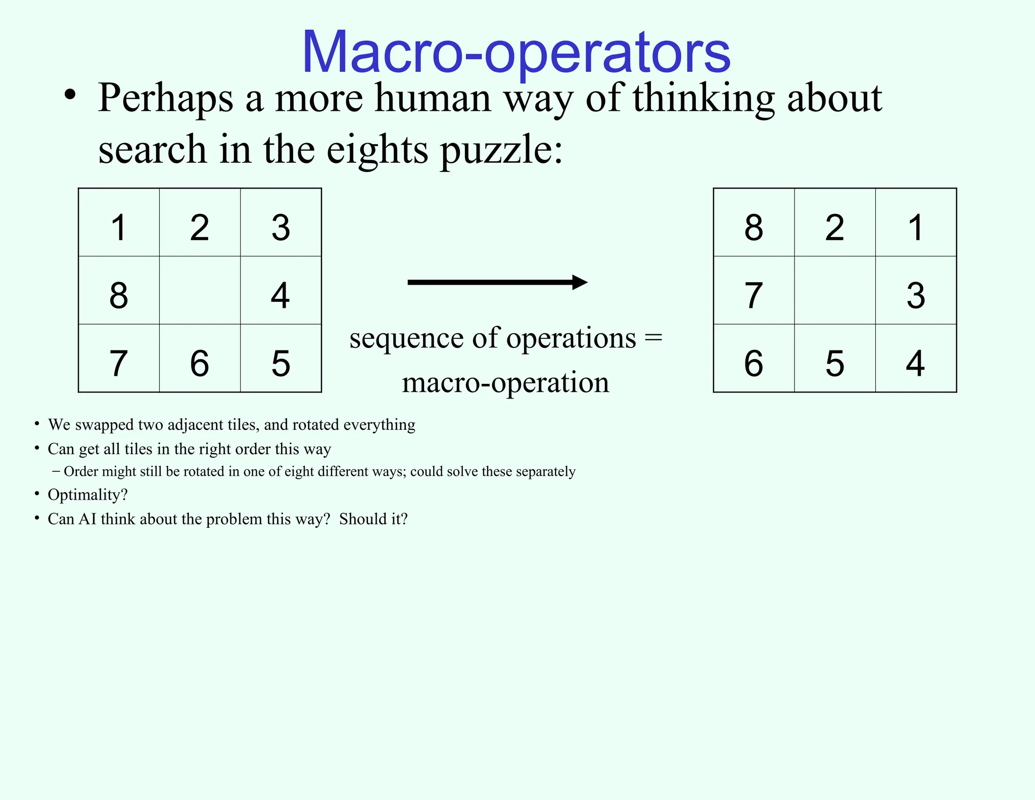
Macro-operators
• Perhaps amore human way of thinking about
search in the eights puzzle:
8 2 1
7 3
6 5 4
1 2 3
8 4
7 6 5
sequence of operations =
macro-operation
• We swapped two adjacent tiles, and rotated everything
• Can get all tiles in the right order this way
– Order might still be rotated in one of eight different ways; could solve these separately
• Optimality?
• Can AI think about the problem this way? Should it?
![Repeated states
• Repeated states can cause incompleteness or enormous
runtimes
• Can maintain list of previously visited states to avoid this
– If new path to the same state has greater cost, don’t pursue it further
– Leads to time/space tradeoff
• “Algorithms that forget their history are doomed to repeat
it” [Russell and Norvig]
A
B
C
3
2
2
cycles exponentially large search trees (try it!)](https://image.slidesharecdn.com/cps270search-250327055519-b5ec6467/75/Different-Search-Techniques-used-in-AI-ppt-25-2048.jpg)


![Repeated states
• Repeated states can cause incompleteness or enormous
runtimes
• Can maintain list of previously visited states to avoid this
– If new path to the same state has greater cost, don’t pursue it further
– Leads to time/space tradeoff
• “Algorithms that forget their history are doomed to repeat
it” [Russell and Norvig]
A
B
C
3
2
2
cycles exponentially large search trees (try it!)](https://crownmelresort.com/image.slidesharecdn.com/cps270search-250327055519-b5ec6467/75/Different-Search-Techniques-used-in-AI-ppt-25-2048.jpg)