Download as PDF, PPTX


![Train the Classifier
• This is the ‘smart interface’ where GraphLab decides
which classifier to us
• Note that the features are simply flow, speed and
occupancy
• Is this model oversimplified?
33
model =
graphlab.classifier.create(final_training_data_d0_2014_1
0_29, target='incident_happened’,
features=['total_flow', 'avg_speed', 'avg_occupancy'])
Prototype the Solution](https://image.slidesharecdn.com/datasciencebasedontrafficdatafinal-150217170119-conversion-gate01/75/Get-Started-with-Data-Science-by-Analyzing-Traffic-Data-from-California-Highways-33-2048.jpg)
![SVM – Results
38
Data:
+--------------+-----------------+-------+
| target_label | predicted_label | count |
+--------------+-----------------+-------+
| 0 | 0 | 3746 |
| 0 | 1 | 12330 |
| 1 | 0 | 3522 |
| 1 | 1 | 3711 |
+--------------+-----------------+-------+
[4 rows x 3 columns]
, 'accuracy': 0.31991934445922177}
Prototype the Solution](https://image.slidesharecdn.com/datasciencebasedontrafficdatafinal-150217170119-conversion-gate01/75/Get-Started-with-Data-Science-by-Analyzing-Traffic-Data-from-California-Highways-38-2048.jpg)
![Boosted Trees – Results
39
Data:
+--------------+-----------------+-------+
| target_label | predicted_label | count |
+--------------+-----------------+-------+
| 0 | 0 | 15082 |
| 0 | 1 | 994 |
| 1 | 0 | 5574 |
| 1 | 1 | 1659 |
+--------------+-----------------+-------+
[4 rows x 3 columns]
, 'accuracy': 0.7182204298768716}
Prototype the Solution](https://image.slidesharecdn.com/datasciencebasedontrafficdatafinal-150217170119-conversion-gate01/75/Get-Started-with-Data-Science-by-Analyzing-Traffic-Data-from-California-Highways-39-2048.jpg)


![Train the Classifier
• This is the ‘smart interface’ where GraphLab decides
which classifier to us
• Note that the features are simply flow, speed and
occupancy
• Is this model oversimplified?
33
model =
graphlab.classifier.create(final_training_data_d0_2014_1
0_29, target='incident_happened’,
features=['total_flow', 'avg_speed', 'avg_occupancy'])
Prototype the Solution](https://crownmelresort.com/image.slidesharecdn.com/datasciencebasedontrafficdatafinal-150217170119-conversion-gate01/75/Get-Started-with-Data-Science-by-Analyzing-Traffic-Data-from-California-Highways-33-2048.jpg)


![SVM – Results
38
Data:
+--------------+-----------------+-------+
| target_label | predicted_label | count |
+--------------+-----------------+-------+
| 0 | 0 | 3746 |
| 0 | 1 | 12330 |
| 1 | 0 | 3522 |
| 1 | 1 | 3711 |
+--------------+-----------------+-------+
[4 rows x 3 columns]
, 'accuracy': 0.31991934445922177}
Prototype the Solution](https://crownmelresort.com/image.slidesharecdn.com/datasciencebasedontrafficdatafinal-150217170119-conversion-gate01/75/Get-Started-with-Data-Science-by-Analyzing-Traffic-Data-from-California-Highways-38-2048.jpg)
![Boosted Trees – Results
39
Data:
+--------------+-----------------+-------+
| target_label | predicted_label | count |
+--------------+-----------------+-------+
| 0 | 0 | 15082 |
| 0 | 1 | 994 |
| 1 | 0 | 5574 |
| 1 | 1 | 1659 |
+--------------+-----------------+-------+
[4 rows x 3 columns]
, 'accuracy': 0.7182204298768716}
Prototype the Solution](https://crownmelresort.com/image.slidesharecdn.com/datasciencebasedontrafficdatafinal-150217170119-conversion-gate01/75/Get-Started-with-Data-Science-by-Analyzing-Traffic-Data-from-California-Highways-39-2048.jpg)


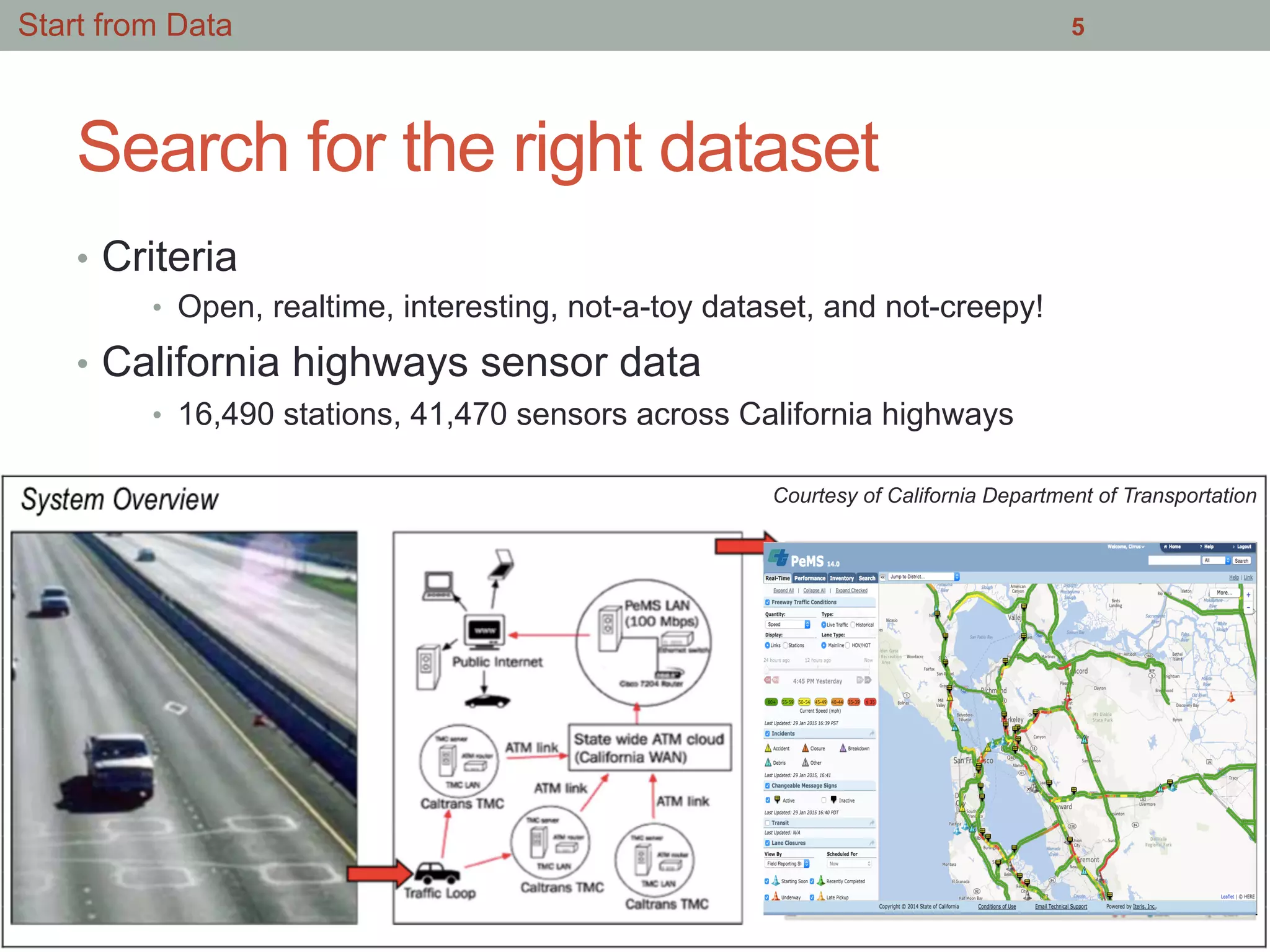
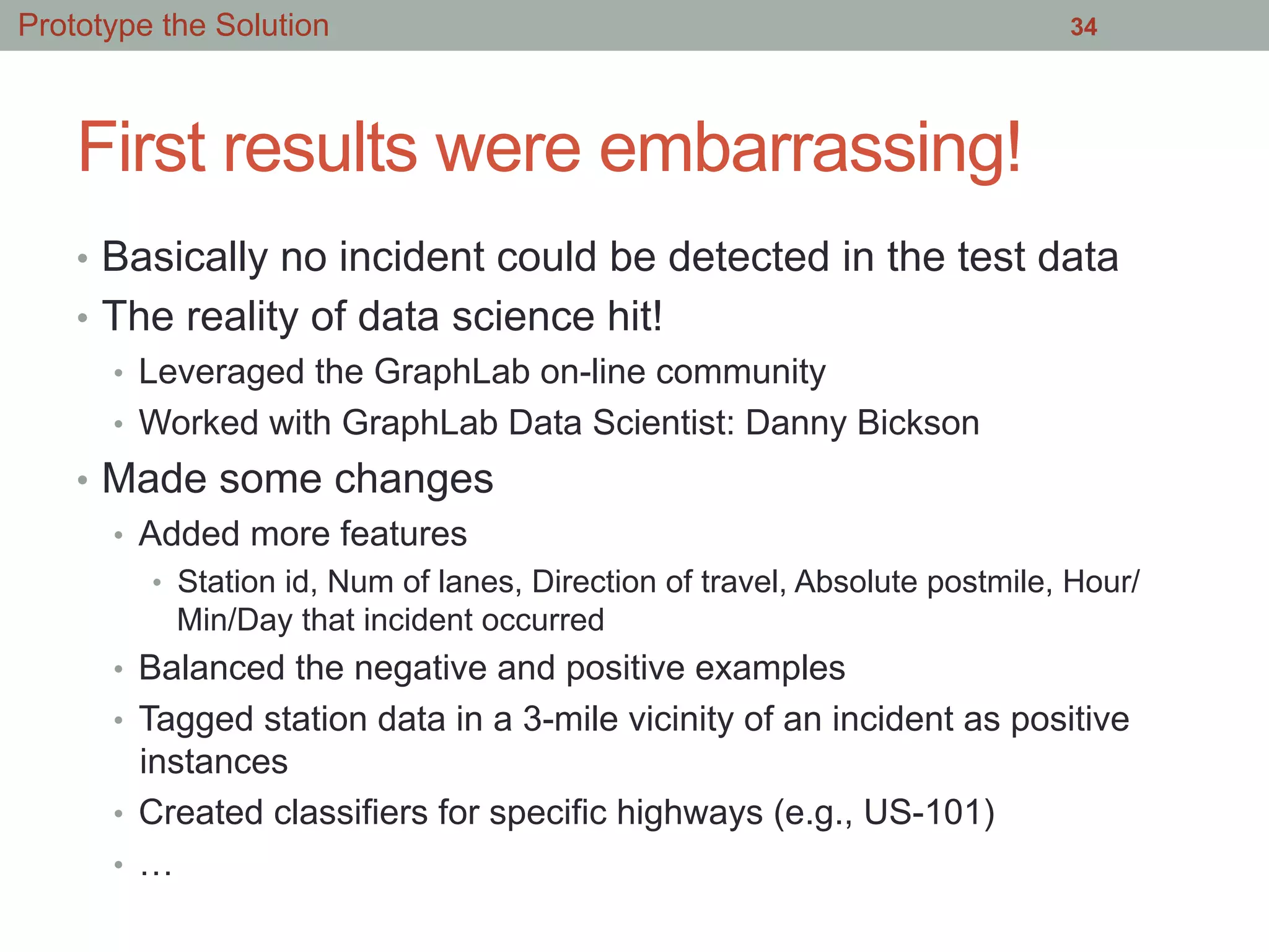
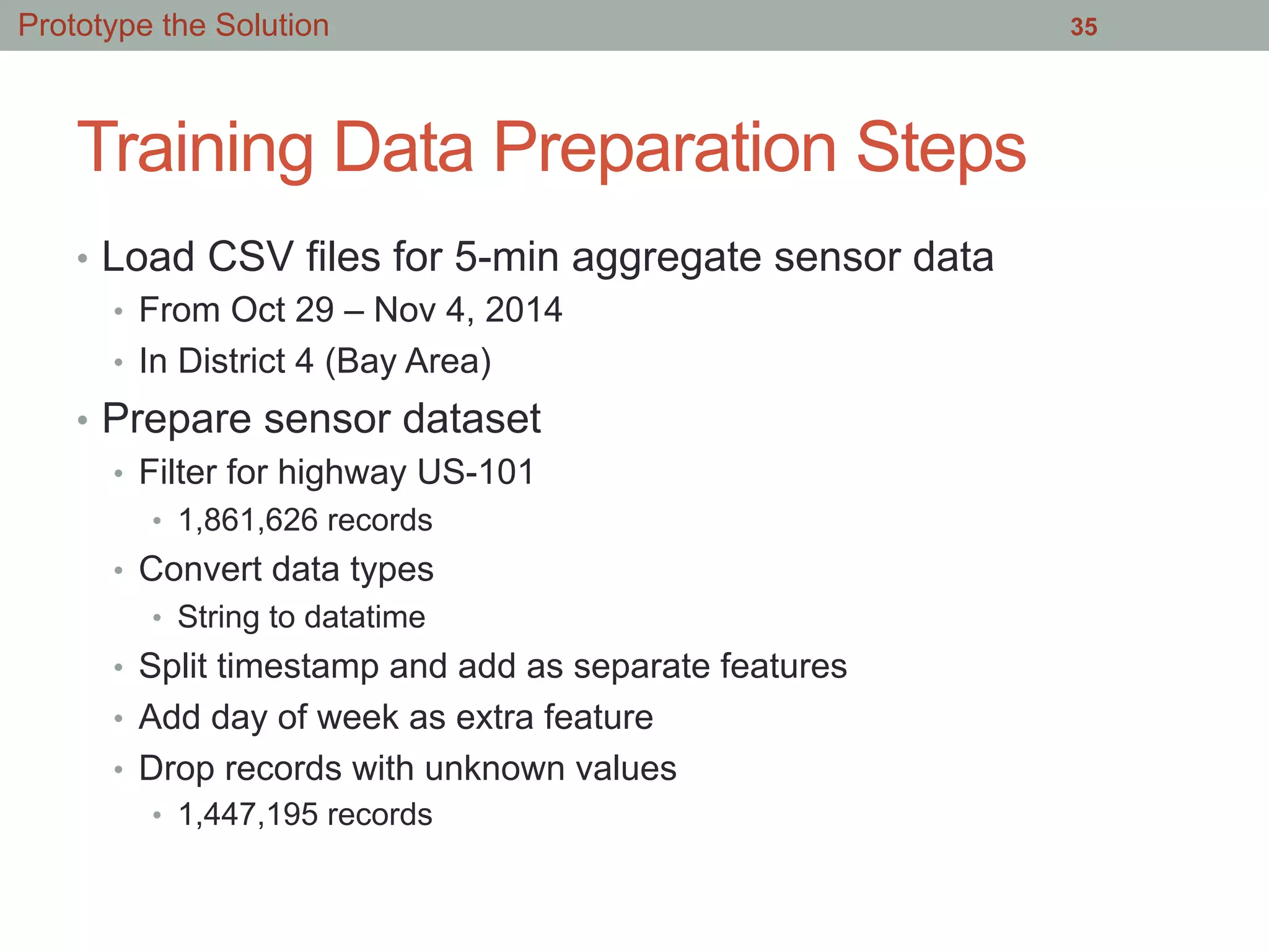
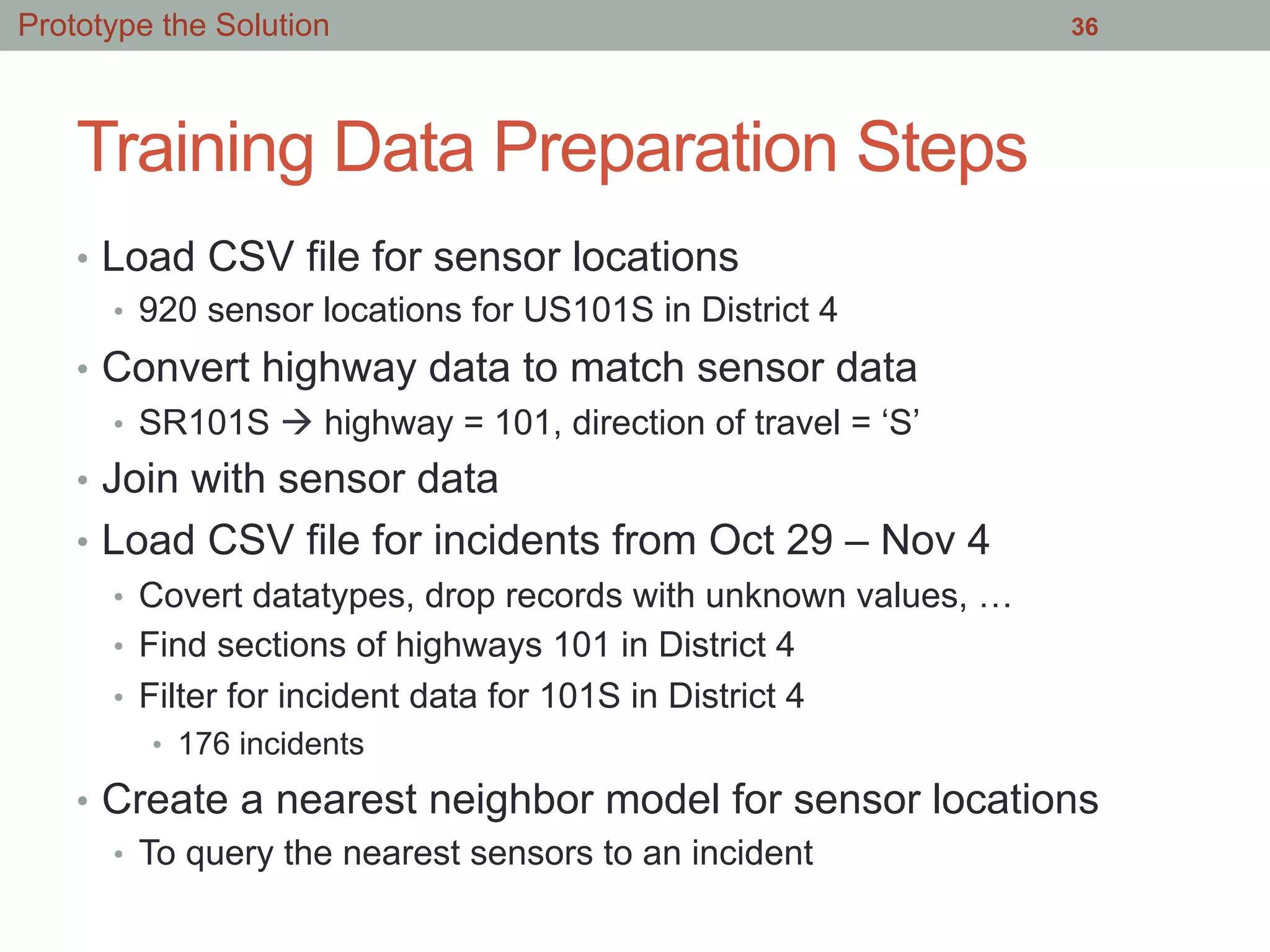
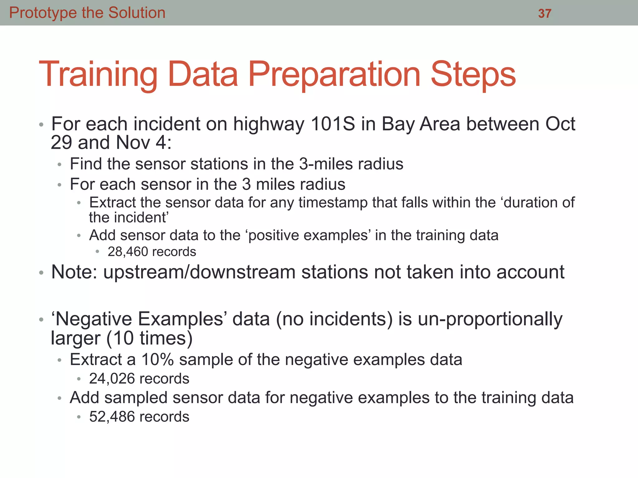
This document summarizes an effort to analyze traffic data from California highways to better understand data science techniques. The researchers searched for an open dataset, eventually finding sensor data from California highways. They analyzed the data format and values to understand it. To detect traffic incidents, they framed it as a classification problem and prepared training data by labeling sensor records near incidents as positive examples. They trained classifiers on this data but initial results were poor. After refining the features and balancing the training data, the classifiers showed more promising results.