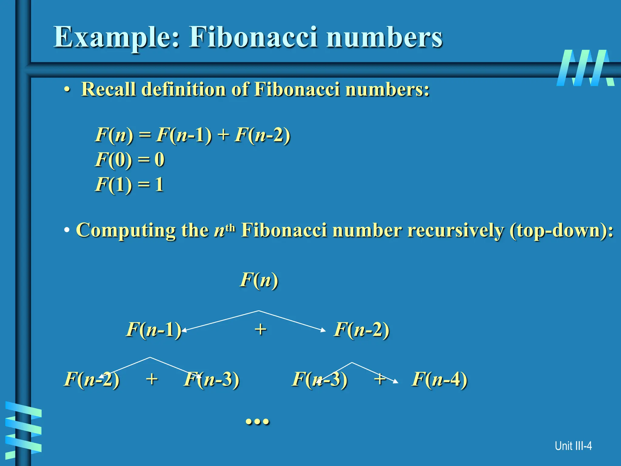
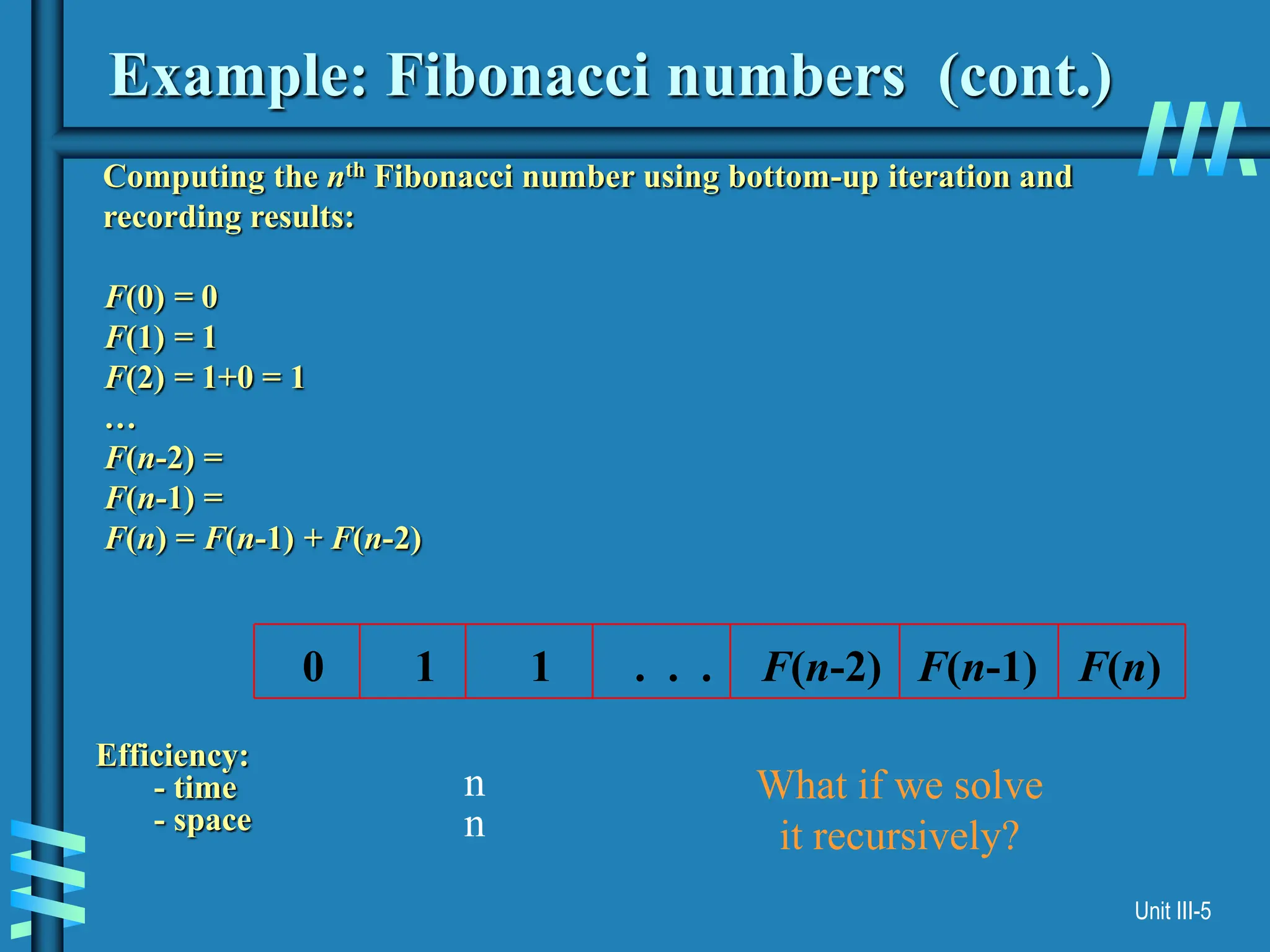
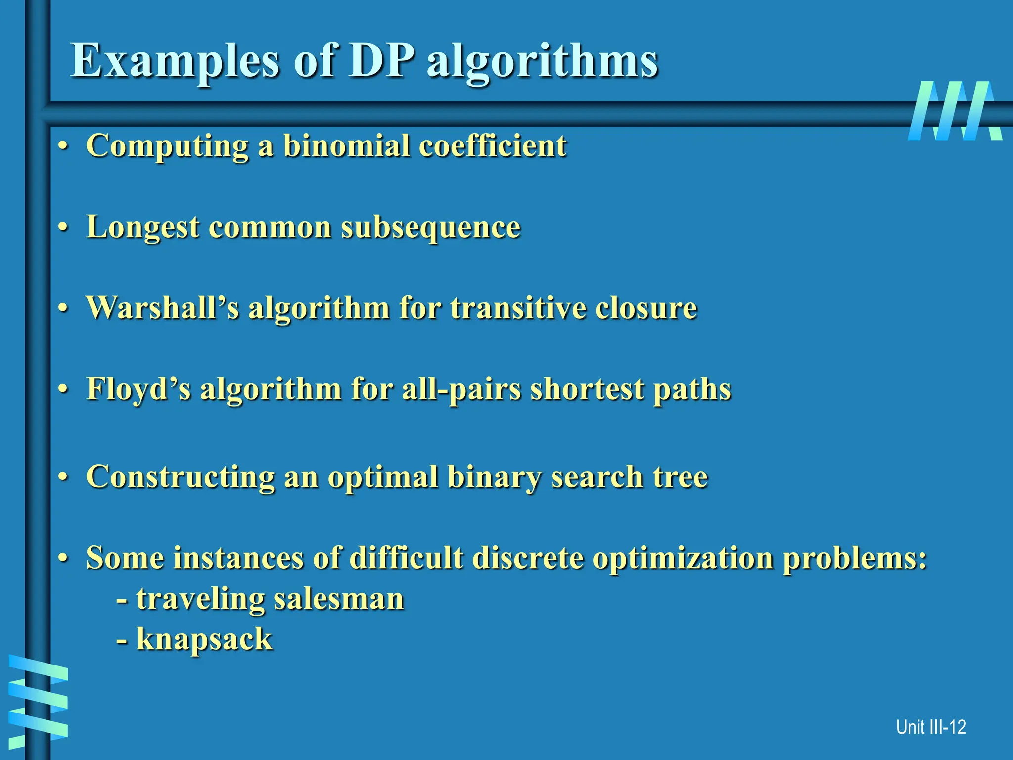
Dynamic programming is a method for solving problems with overlapping sub-problems by solving each sub-problem once and storing the results. This technique, introduced by Richard Bellman, can employ either a bottom-up or a top-down approach to efficiently compute solutions. Examples of problems that can be solved using dynamic programming include Fibonacci numbers, binomial coefficients, and various optimization problems like the traveling salesman and knapsack problem.


![Unit III-11
Top-Down
suppose we have a simple map object, m, which maps each
value of Fibo that has already been calculated to its result,
and we modify our function to use it and update it. The
resulting function requires only O(n) time instead of
exponential time:
This technique of saving values that have already been
calculated is called Memory Function; this is the top-down
approach, since we first break the problem into
subproblems and then calculate and store values
m [0] = 0
m [1] = 1
Algorithm Fibo(n)
if map m does not contain key n
m[n] := Fibo(n − 1) + Fibo(n − 2)
return m[n]](https://image.slidesharecdn.com/d0a2de03-27d3-4ca2-9ac6-d83440657a6c-240722185120-e0ea553c/75/d0a2de03-27d3-4ca2-9ac6-d83440657a6c-ppt-12-2048.jpg)
![Unit III-16
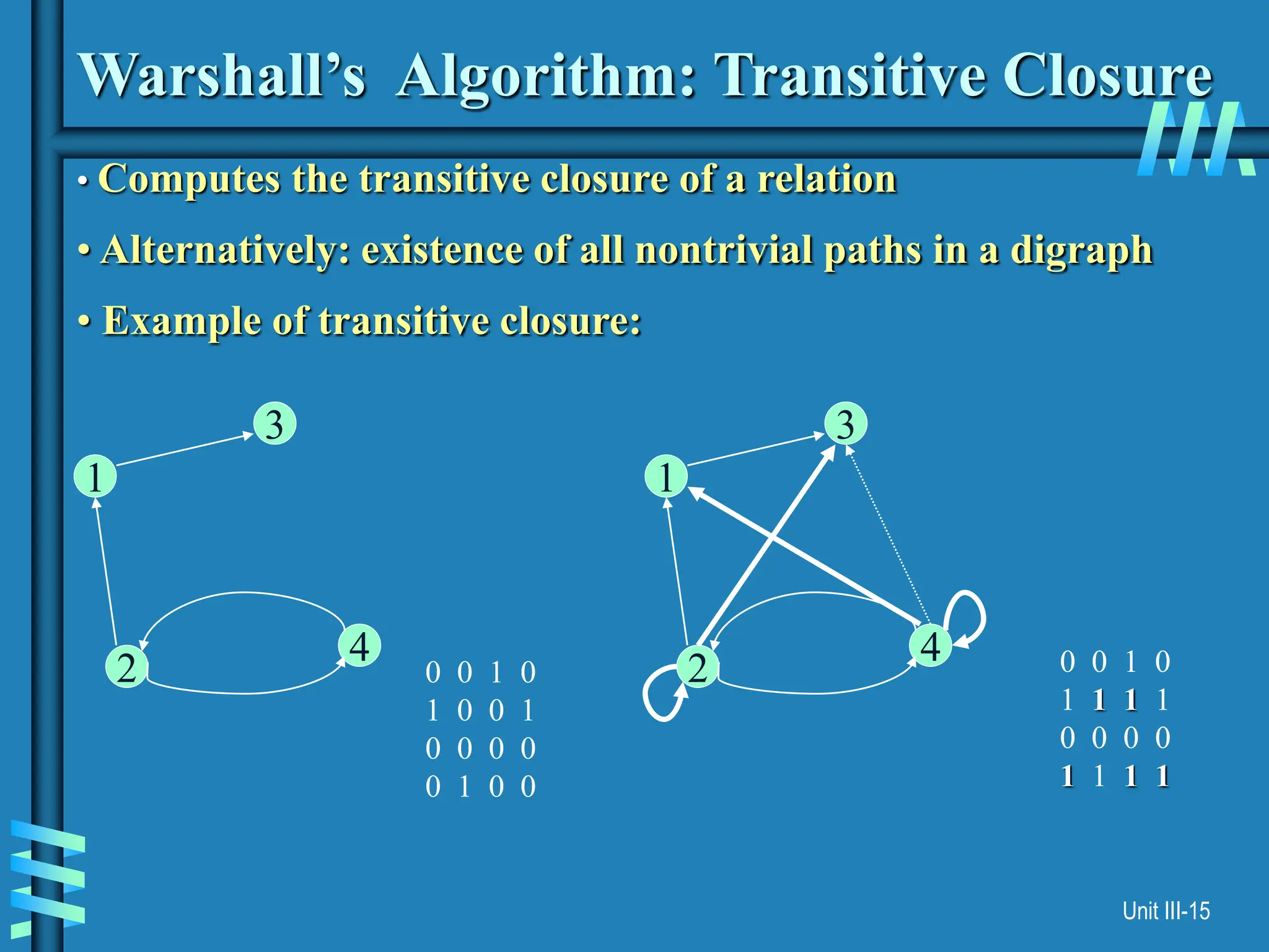
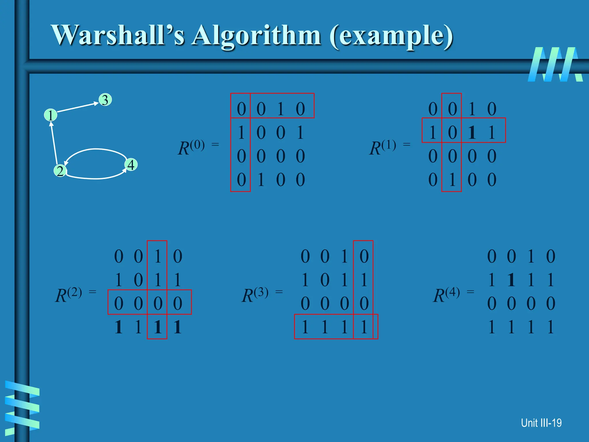
Warshall’s Algorithm
Constructs transitive closure T as the last matrix in the sequence
of n-by-n matrices R(0), … , R(k), … , R(n) where
R(k)[i,j] = 1 iff there is nontrivial path from i to j with only the
first k vertices allowed as intermediate
Note that R(0) = A (adjacency matrix), R(n) = T (transitive closure)
3
4
2
1
3
4
2
1
3
4
2
1
3
4
2
1
R(0)
0 0 1 0
1 0 0 1
0 0 0 0
0 1 0 0
R(1)
0 0 1 0
1 0 1 1
0 0 0 0
0 1 0 0
R(2)
0 0 1 0
1 0 1 1
0 0 0 0
1 1 1 1
R(3)
0 0 1 0
1 0 1 1
0 0 0 0
1 1 1 1
R(4)
0 0 1 0
1 1 1 1
0 0 0 0
1 1 1 1
3
4
2
1](https://image.slidesharecdn.com/d0a2de03-27d3-4ca2-9ac6-d83440657a6c-240722185120-e0ea553c/75/d0a2de03-27d3-4ca2-9ac6-d83440657a6c-ppt-17-2048.jpg)
![Unit III-17
Warshall’s Algorithm (recurrence)
On the k-th iteration, the algorithm determines for every pair of
vertices i, j if a path exists from i and j with just vertices 1,…,k
allowed as intermediate
R(k-1)[i,j] (path using just 1 ,…,k-1)
R(k)[i,j] = or
R(k-1)[i,k] and R(k-1)[k,j] (path from i to k
and from k to j
using just 1 ,…,k-1)
i
j
k
{
Initial condition?](https://image.slidesharecdn.com/d0a2de03-27d3-4ca2-9ac6-d83440657a6c-240722185120-e0ea553c/75/d0a2de03-27d3-4ca2-9ac6-d83440657a6c-ppt-18-2048.jpg)
![Unit III-18
Warshall’s Algorithm (matrix generation)
Recurrence relating elements R(k) to elements of R(k-1) is:
R(k)[i,j] = R(k-1)[i,j] or (R(k-1)[i,k] and R(k-1)[k,j])
It implies the following rules for generating R(k) from R(k-1):
Rule 1 If an element in row i and column j is 1 in R(k-1),
it remains 1 in R(k)
Rule 2 If an element in row i and column j is 0 in R(k-1),
it has to be changed to 1 in R(k) if and only if
the element in its row i and column k and the element
in its column j and row k are both 1’s in R(k-1)](https://image.slidesharecdn.com/d0a2de03-27d3-4ca2-9ac6-d83440657a6c-240722185120-e0ea553c/75/d0a2de03-27d3-4ca2-9ac6-d83440657a6c-ppt-19-2048.jpg)

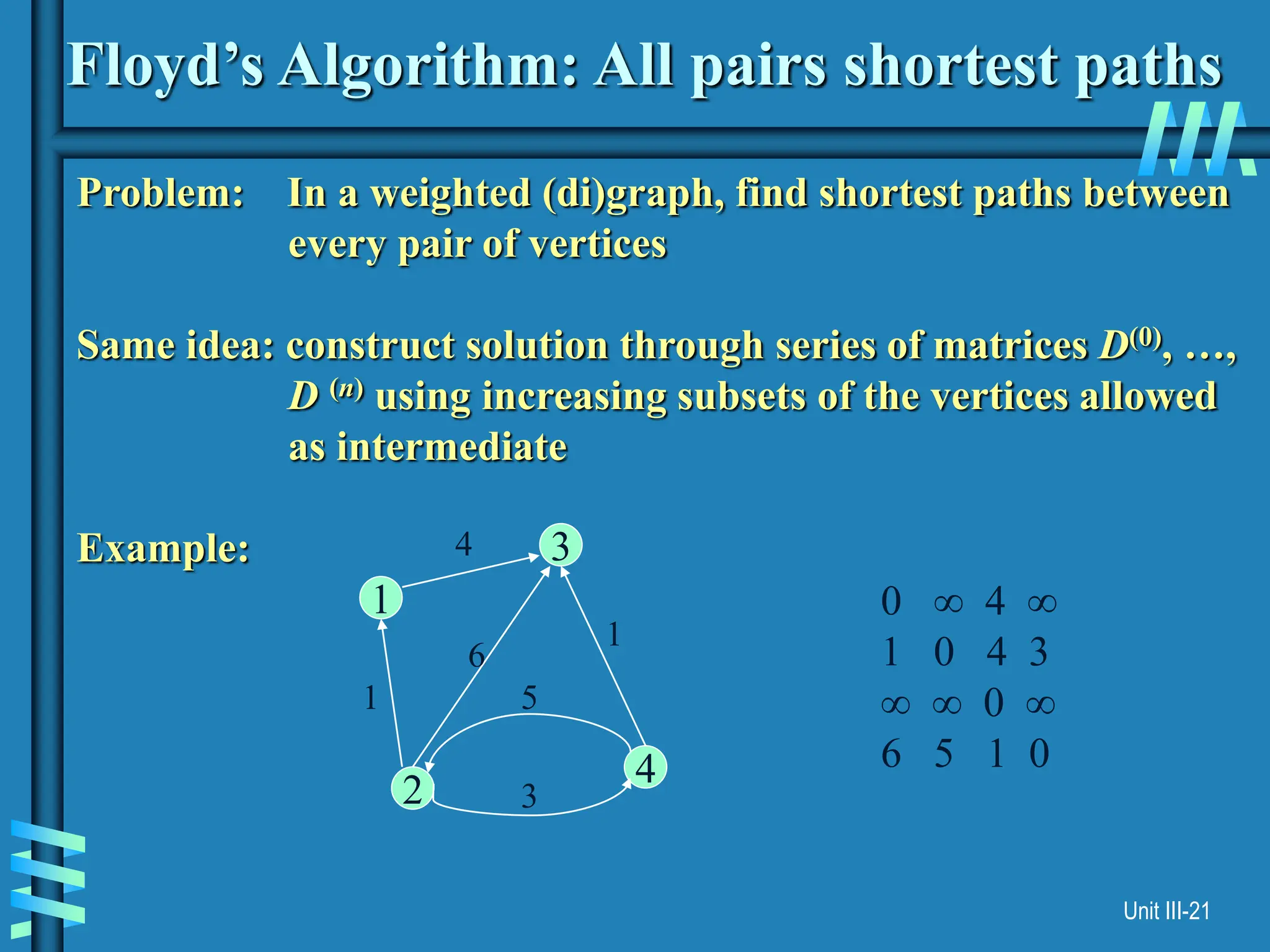
![Unit III-22
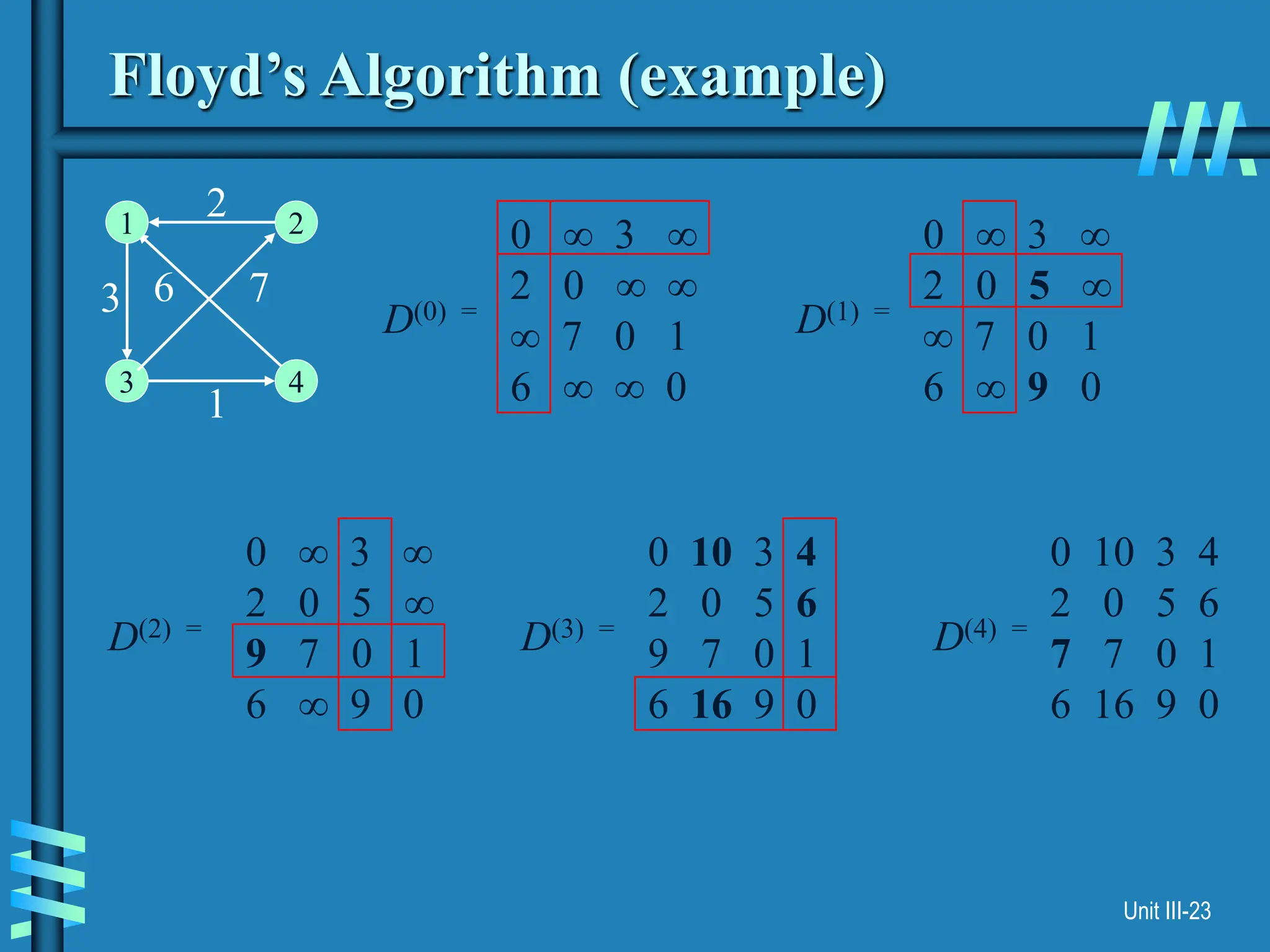
Floyd’s Algorithm (matrix generation)
On the k-th iteration, the algorithm determines shortest paths
between every pair of vertices i, j that use only vertices among
1,…,k as intermediate
D(k)[i,j] = min {D(k-1)[i,j], D(k-1)[i,k] + D(k-1)[k,j]}
i
j
k
D(k-1)[i,j]
D(k-1)[i,k]
D(k-1)[k,j]
Initial condition?](https://image.slidesharecdn.com/d0a2de03-27d3-4ca2-9ac6-d83440657a6c-240722185120-e0ea553c/75/d0a2de03-27d3-4ca2-9ac6-d83440657a6c-ppt-23-2048.jpg)
![Unit III-24
Floyd’s Algorithm (pseudocode and analysis)
Time efficiency: Θ(n3)
Space efficiency: Matrices can be written over their predecessors
Note: Works on graphs with negative edges but without negative cycles.
Shortest paths themselves can be found, too. How?
If D[i,k] + D[k,j] < D[i,j] then P[i,j] k
Since the superscripts k or k-1 make
no difference to D[i,k] and D[k,j].](https://image.slidesharecdn.com/d0a2de03-27d3-4ca2-9ac6-d83440657a6c-240722185120-e0ea553c/75/d0a2de03-27d3-4ca2-9ac6-d83440657a6c-ppt-25-2048.jpg)
![Unit III-26
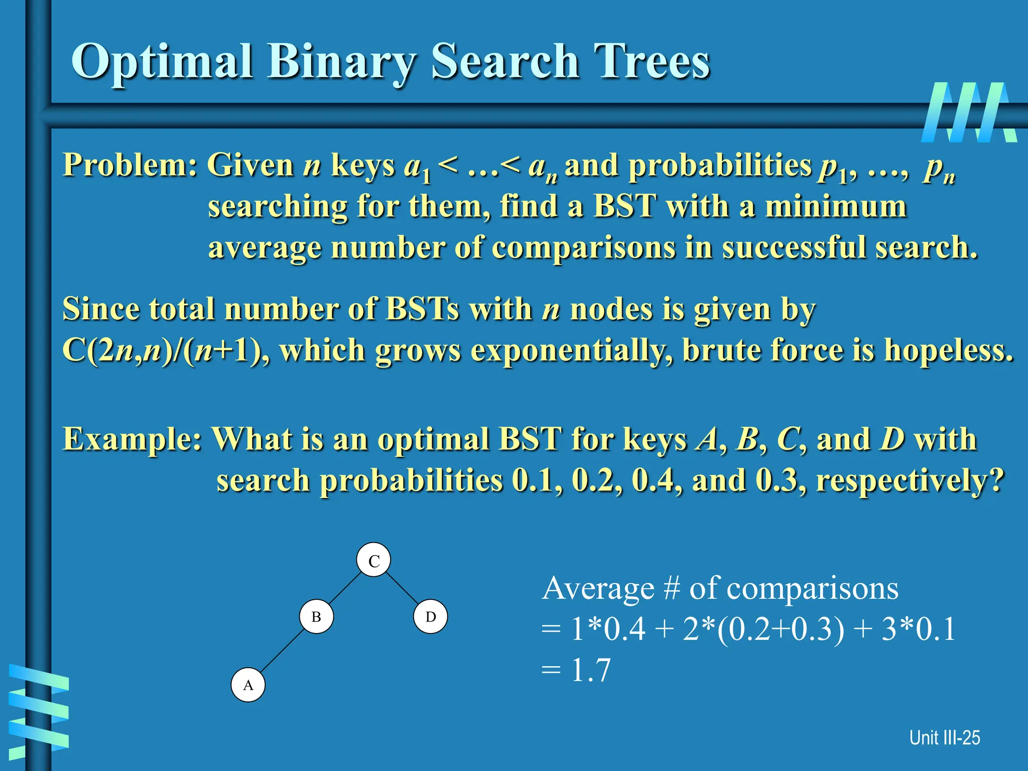
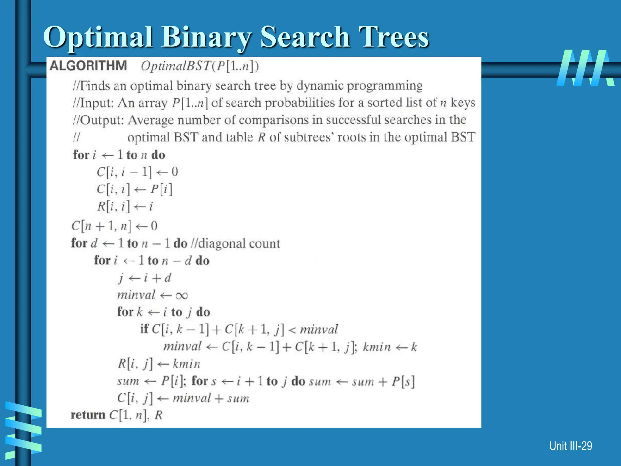
DP for Optimal BST Problem
Let C[i,j] be minimum average number of comparisons made in
T[i,j], optimal BST for keys ai < …< aj , where 1 ≤ i ≤ j ≤ n.
Consider optimal BST among all BSTs with some ak (i ≤ k ≤ j )
as their root; T[i,j] is the best among them.
a
Optimal
BST for
a , ..., a
Optimal
BST for
a , ..., a
i
k
k-1 k+1 j
C[i,j] =
min {pk · 1 +
∑ ps (level as in T[i,k-1] +1) +
∑ ps (level as in T[k+1,j] +1)}
i ≤ k ≤ j
s = i
k-1
s =k+1
j](https://image.slidesharecdn.com/d0a2de03-27d3-4ca2-9ac6-d83440657a6c-240722185120-e0ea553c/75/d0a2de03-27d3-4ca2-9ac6-d83440657a6c-ppt-27-2048.jpg)
![Unit III-27
goal
0
0
C[i,j]
0
1
n+1
0 1 n
p 1
p2
n
p
i
j
DP for Optimal BST Problem (cont.)
After simplifications, we obtain the recurrence for C[i,j]:
C[i,j] = min {C[i,k-1] + C[k+1,j]} + ∑ ps for 1 ≤ i ≤ j ≤ n
C[i,i] = pi for 1 ≤ i ≤ j ≤ n
s = i
j
i ≤ k ≤ j](https://image.slidesharecdn.com/d0a2de03-27d3-4ca2-9ac6-d83440657a6c-240722185120-e0ea553c/75/d0a2de03-27d3-4ca2-9ac6-d83440657a6c-ppt-28-2048.jpg)
![Example: key A B C D
probability 0.1 0.2 0.4 0.3
The tables below are filled diagonal by diagonal: the left one is filled
using the recurrence
C[i,j] = min {C[i,k-1] + C[k+1,j]} + ∑ ps , C[i,i] = pi ;
the right one, for trees’ roots, records k’s values giving the minima
0 1 2 3 4
1 0 .1 .4 1.1 1.7
2 0 .2 .8 1.4
3 0 .4 1.0
4 0 .3
5 0
0 1 2 3 4
1 1 2 3 3
2 2 3 3
3 3 3
4 4
5
i ≤ k ≤ j s = i
j
optimal BST
B
A
C
D
i
j
i
j](https://image.slidesharecdn.com/d0a2de03-27d3-4ca2-9ac6-d83440657a6c-240722185120-e0ea553c/75/d0a2de03-27d3-4ca2-9ac6-d83440657a6c-ppt-29-2048.jpg)
![Unit III-30
Analysis DP for Optimal BST Problem
Time efficiency: Θ(n3) but can be reduced to Θ(n2) by taking
advantage of monotonicity of entries in the
root table, i.e., R[i,j] is always in the range
between R[i,j-1] and R[i+1,j]
Space efficiency: Θ(n2)
Method can be expanded to include unsuccessful searches](https://image.slidesharecdn.com/d0a2de03-27d3-4ca2-9ac6-d83440657a6c-240722185120-e0ea553c/75/d0a2de03-27d3-4ca2-9ac6-d83440657a6c-ppt-31-2048.jpg)
![Unit III-31
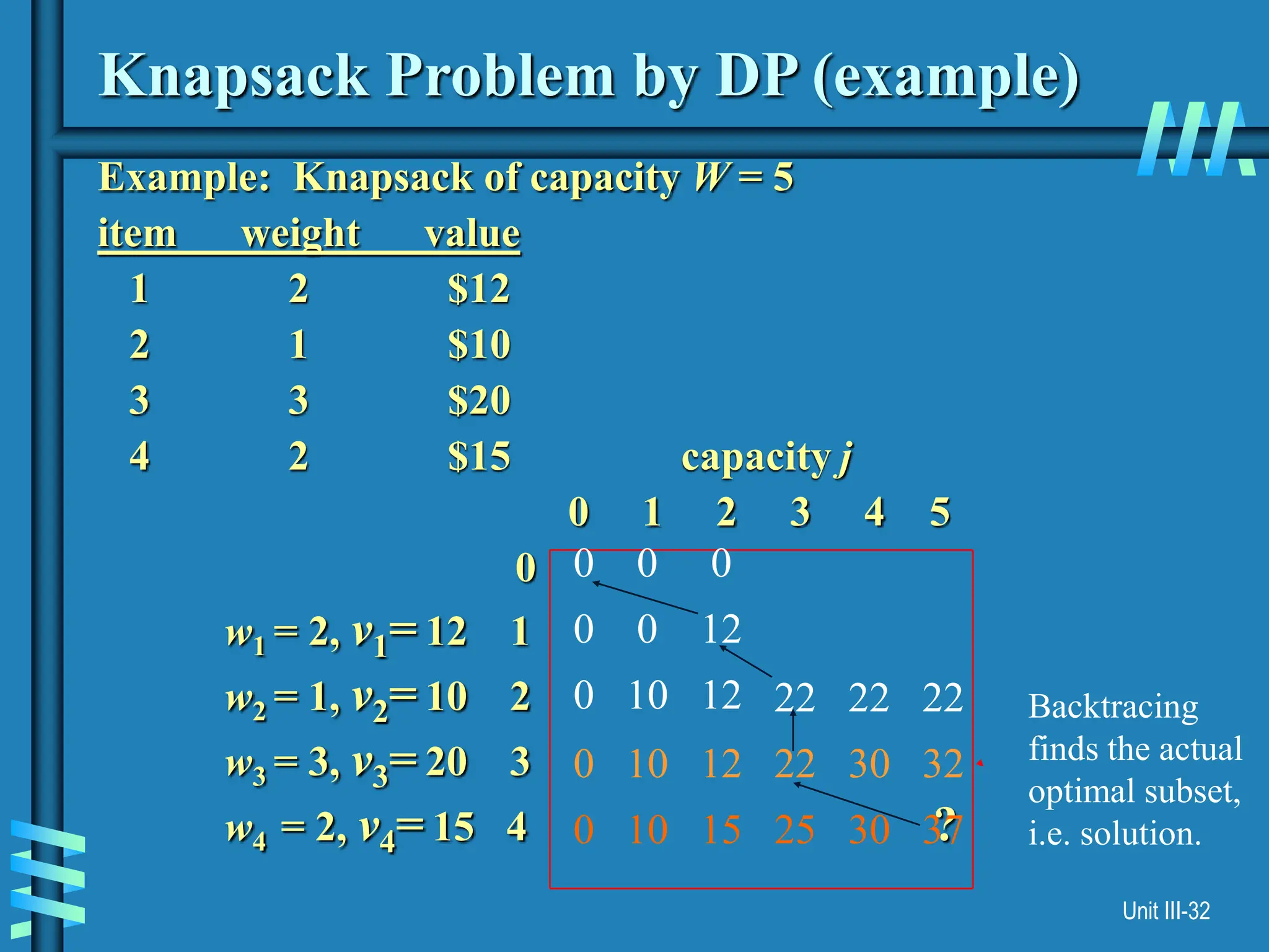
Knapsack Problem by DP
Given n items of
integer weights: w1 w2 … wn
values: v1 v2 … vn
a knapsack of integer capacity W
find most valuable subset of the items that fit into the knapsack
Consider instance defined by first i items and capacity j (j W).
Let V[i,j] be optimal value of such an instance. Then
max {V[i-1,j], vi + V[i-1,j- wi]} if j- wi 0
V[i,j] =
V[i-1,j] if j- wi < 0
Initial conditions: V[0,j] = 0 and V[i,0] = 0
{](https://image.slidesharecdn.com/d0a2de03-27d3-4ca2-9ac6-d83440657a6c-240722185120-e0ea553c/75/d0a2de03-27d3-4ca2-9ac6-d83440657a6c-ppt-32-2048.jpg)
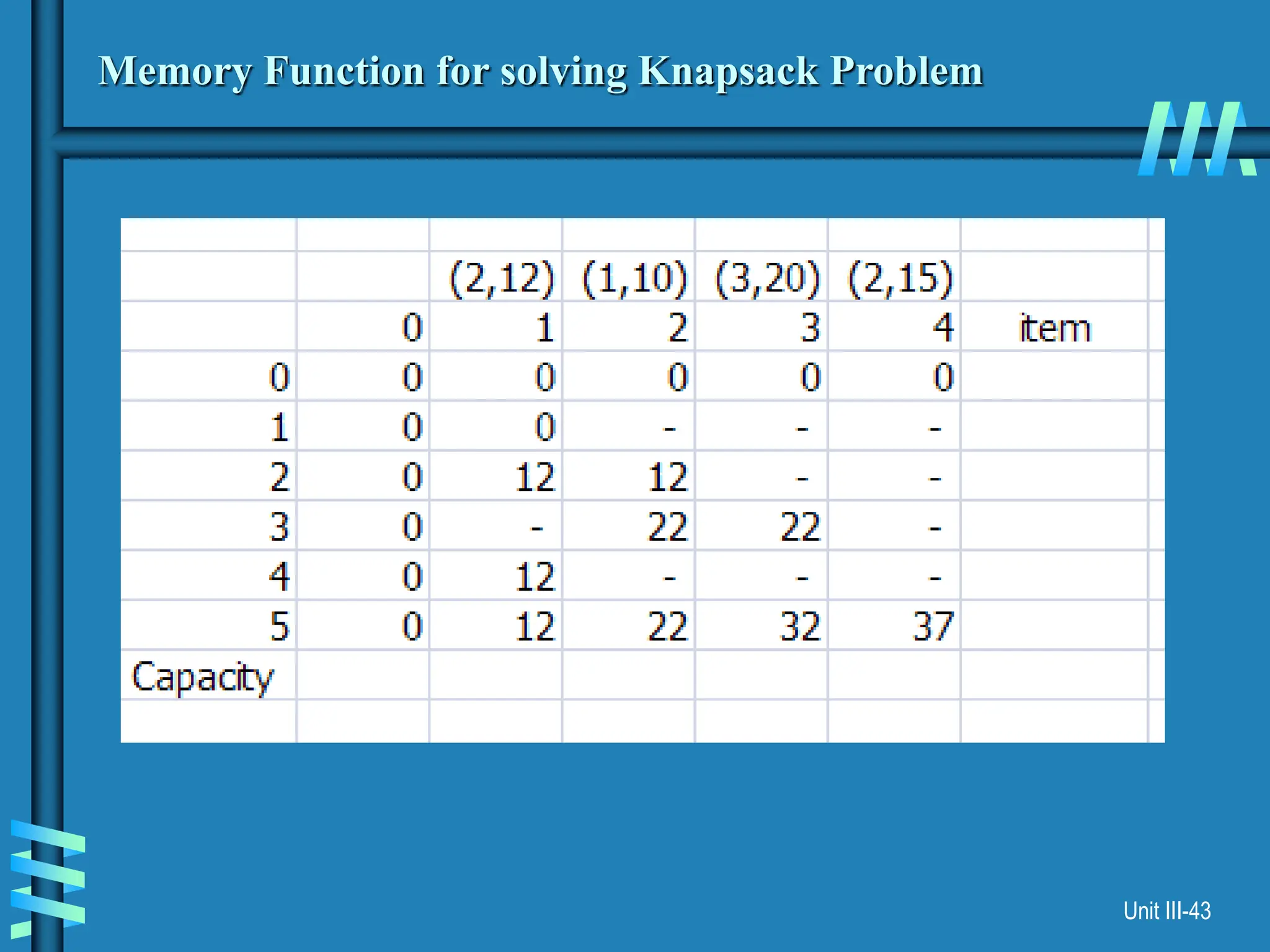
![Unit III-34
Example
Thus, the maximal value is V [4, 5]= $37. We can find the
composition of an optimal subset by tracing back the
computations of this entry in the table.
Since V [4, 5] is not equal to V [3, 5], item 4 was included in an
optimal solution along with an optimal subset for filling 5 - 2 = 3
remaining units of the knapsack capacity.
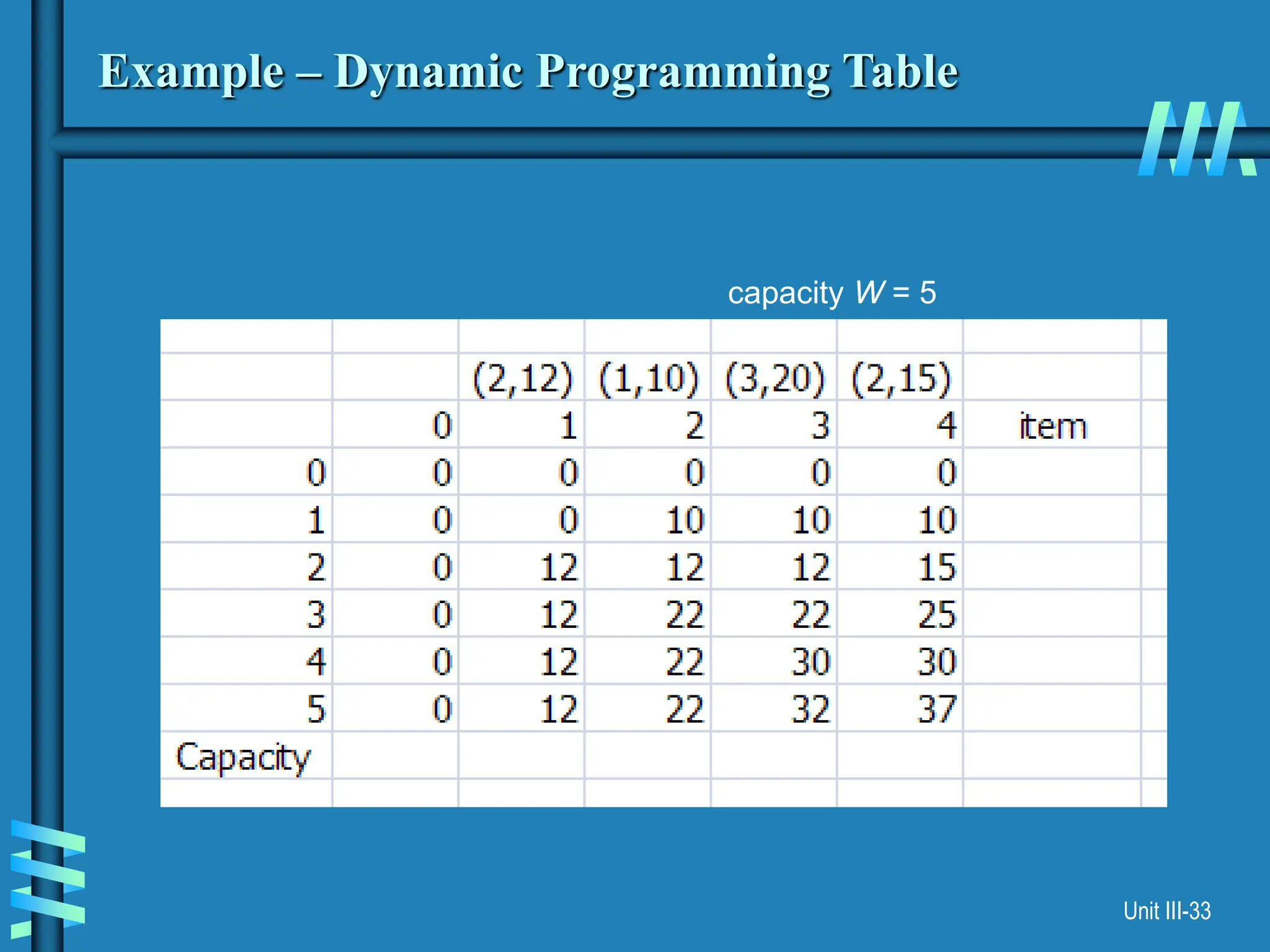
capacity W = 5](https://image.slidesharecdn.com/d0a2de03-27d3-4ca2-9ac6-d83440657a6c-240722185120-e0ea553c/75/d0a2de03-27d3-4ca2-9ac6-d83440657a6c-ppt-35-2048.jpg)
![Unit III-35
Example
The remaining is V[3,3]
Here V[3,3] = V[2,3] so item 3 is not included
V[2,3] V[1,3] so item 2 is included
capacity W = 5](https://image.slidesharecdn.com/d0a2de03-27d3-4ca2-9ac6-d83440657a6c-240722185120-e0ea553c/75/d0a2de03-27d3-4ca2-9ac6-d83440657a6c-ppt-36-2048.jpg)
![Unit III-36
Example
The remaining is V[1,2]
V[1,2] V[0,2] so item 1 is included
The solution is {item 1, item 2, item 4}
Total weight is 5
Total value is 37
capacity W = 5](https://image.slidesharecdn.com/d0a2de03-27d3-4ca2-9ac6-d83440657a6c-240722185120-e0ea553c/75/d0a2de03-27d3-4ca2-9ac6-d83440657a6c-ppt-37-2048.jpg)

![Unit III-38
Knapsack Problem by DP (pseudocode)
Algorithm DPKnapsack(w[1..n], v[1..n], W)
var V[0..n,0..W], P[1..n,1..W]: int
for j := 0 to W do
V[0,j] := 0
for i := 0 to n do
V[i,0] := 0
for i := 1 to n do
for j := 1 to W do
if w[i] j and v[i] + V[i-1,j-w[i]] > V[i-1,j] then
V[i,j] := v[i] + V[i-1,j-w[i]]; P[i,j] := j-w[i]
else
V[i,j] := V[i-1,j]; P[i,j] := j
return V[n,W] and the optimal subset by backtracing
Running time and space:
O(nW).](https://image.slidesharecdn.com/d0a2de03-27d3-4ca2-9ac6-d83440657a6c-240722185120-e0ea553c/75/d0a2de03-27d3-4ca2-9ac6-d83440657a6c-ppt-39-2048.jpg)


![Unit III-11
Top-Down
suppose we have a simple map object, m, which maps each
value of Fibo that has already been calculated to its result,
and we modify our function to use it and update it. The
resulting function requires only O(n) time instead of
exponential time:
This technique of saving values that have already been
calculated is called Memory Function; this is the top-down
approach, since we first break the problem into
subproblems and then calculate and store values
m [0] = 0
m [1] = 1
Algorithm Fibo(n)
if map m does not contain key n
m[n] := Fibo(n − 1) + Fibo(n − 2)
return m[n]](https://crownmelresort.com/image.slidesharecdn.com/d0a2de03-27d3-4ca2-9ac6-d83440657a6c-240722185120-e0ea553c/75/d0a2de03-27d3-4ca2-9ac6-d83440657a6c-ppt-12-2048.jpg)


![Unit III-16
Warshall’s Algorithm
Constructs transitive closure T as the last matrix in the sequence
of n-by-n matrices R(0), … , R(k), … , R(n) where
R(k)[i,j] = 1 iff there is nontrivial path from i to j with only the
first k vertices allowed as intermediate
Note that R(0) = A (adjacency matrix), R(n) = T (transitive closure)
3
4
2
1
3
4
2
1
3
4
2
1
3
4
2
1
R(0)
0 0 1 0
1 0 0 1
0 0 0 0
0 1 0 0
R(1)
0 0 1 0
1 0 1 1
0 0 0 0
0 1 0 0
R(2)
0 0 1 0
1 0 1 1
0 0 0 0
1 1 1 1
R(3)
0 0 1 0
1 0 1 1
0 0 0 0
1 1 1 1
R(4)
0 0 1 0
1 1 1 1
0 0 0 0
1 1 1 1
3
4
2
1](https://crownmelresort.com/image.slidesharecdn.com/d0a2de03-27d3-4ca2-9ac6-d83440657a6c-240722185120-e0ea553c/75/d0a2de03-27d3-4ca2-9ac6-d83440657a6c-ppt-17-2048.jpg)
![Unit III-17
Warshall’s Algorithm (recurrence)
On the k-th iteration, the algorithm determines for every pair of
vertices i, j if a path exists from i and j with just vertices 1,…,k
allowed as intermediate
R(k-1)[i,j] (path using just 1 ,…,k-1)
R(k)[i,j] = or
R(k-1)[i,k] and R(k-1)[k,j] (path from i to k
and from k to j
using just 1 ,…,k-1)
i
j
k
{
Initial condition?](https://crownmelresort.com/image.slidesharecdn.com/d0a2de03-27d3-4ca2-9ac6-d83440657a6c-240722185120-e0ea553c/75/d0a2de03-27d3-4ca2-9ac6-d83440657a6c-ppt-18-2048.jpg)
![Unit III-18
Warshall’s Algorithm (matrix generation)
Recurrence relating elements R(k) to elements of R(k-1) is:
R(k)[i,j] = R(k-1)[i,j] or (R(k-1)[i,k] and R(k-1)[k,j])
It implies the following rules for generating R(k) from R(k-1):
Rule 1 If an element in row i and column j is 1 in R(k-1),
it remains 1 in R(k)
Rule 2 If an element in row i and column j is 0 in R(k-1),
it has to be changed to 1 in R(k) if and only if
the element in its row i and column k and the element
in its column j and row k are both 1’s in R(k-1)](https://crownmelresort.com/image.slidesharecdn.com/d0a2de03-27d3-4ca2-9ac6-d83440657a6c-240722185120-e0ea553c/75/d0a2de03-27d3-4ca2-9ac6-d83440657a6c-ppt-19-2048.jpg)


![Unit III-22
Floyd’s Algorithm (matrix generation)
On the k-th iteration, the algorithm determines shortest paths
between every pair of vertices i, j that use only vertices among
1,…,k as intermediate
D(k)[i,j] = min {D(k-1)[i,j], D(k-1)[i,k] + D(k-1)[k,j]}
i
j
k
D(k-1)[i,j]
D(k-1)[i,k]
D(k-1)[k,j]
Initial condition?](https://crownmelresort.com/image.slidesharecdn.com/d0a2de03-27d3-4ca2-9ac6-d83440657a6c-240722185120-e0ea553c/75/d0a2de03-27d3-4ca2-9ac6-d83440657a6c-ppt-23-2048.jpg)

![Unit III-24
Floyd’s Algorithm (pseudocode and analysis)
Time efficiency: Θ(n3)
Space efficiency: Matrices can be written over their predecessors
Note: Works on graphs with negative edges but without negative cycles.
Shortest paths themselves can be found, too. How?
If D[i,k] + D[k,j] < D[i,j] then P[i,j] k
Since the superscripts k or k-1 make
no difference to D[i,k] and D[k,j].](https://crownmelresort.com/image.slidesharecdn.com/d0a2de03-27d3-4ca2-9ac6-d83440657a6c-240722185120-e0ea553c/75/d0a2de03-27d3-4ca2-9ac6-d83440657a6c-ppt-25-2048.jpg)

![Unit III-26
DP for Optimal BST Problem
Let C[i,j] be minimum average number of comparisons made in
T[i,j], optimal BST for keys ai < …< aj , where 1 ≤ i ≤ j ≤ n.
Consider optimal BST among all BSTs with some ak (i ≤ k ≤ j )
as their root; T[i,j] is the best among them.
a
Optimal
BST for
a , ..., a
Optimal
BST for
a , ..., a
i
k
k-1 k+1 j
C[i,j] =
min {pk · 1 +
∑ ps (level as in T[i,k-1] +1) +
∑ ps (level as in T[k+1,j] +1)}
i ≤ k ≤ j
s = i
k-1
s =k+1
j](https://crownmelresort.com/image.slidesharecdn.com/d0a2de03-27d3-4ca2-9ac6-d83440657a6c-240722185120-e0ea553c/75/d0a2de03-27d3-4ca2-9ac6-d83440657a6c-ppt-27-2048.jpg)
![Unit III-27
goal
0
0
C[i,j]
0
1
n+1
0 1 n
p 1
p2
n
p
i
j
DP for Optimal BST Problem (cont.)
After simplifications, we obtain the recurrence for C[i,j]:
C[i,j] = min {C[i,k-1] + C[k+1,j]} + ∑ ps for 1 ≤ i ≤ j ≤ n
C[i,i] = pi for 1 ≤ i ≤ j ≤ n
s = i
j
i ≤ k ≤ j](https://crownmelresort.com/image.slidesharecdn.com/d0a2de03-27d3-4ca2-9ac6-d83440657a6c-240722185120-e0ea553c/75/d0a2de03-27d3-4ca2-9ac6-d83440657a6c-ppt-28-2048.jpg)
![Example: key A B C D
probability 0.1 0.2 0.4 0.3
The tables below are filled diagonal by diagonal: the left one is filled
using the recurrence
C[i,j] = min {C[i,k-1] + C[k+1,j]} + ∑ ps , C[i,i] = pi ;
the right one, for trees’ roots, records k’s values giving the minima
0 1 2 3 4
1 0 .1 .4 1.1 1.7
2 0 .2 .8 1.4
3 0 .4 1.0
4 0 .3
5 0
0 1 2 3 4
1 1 2 3 3
2 2 3 3
3 3 3
4 4
5
i ≤ k ≤ j s = i
j
optimal BST
B
A
C
D
i
j
i
j](https://crownmelresort.com/image.slidesharecdn.com/d0a2de03-27d3-4ca2-9ac6-d83440657a6c-240722185120-e0ea553c/75/d0a2de03-27d3-4ca2-9ac6-d83440657a6c-ppt-29-2048.jpg)

![Unit III-30
Analysis DP for Optimal BST Problem
Time efficiency: Θ(n3) but can be reduced to Θ(n2) by taking
advantage of monotonicity of entries in the
root table, i.e., R[i,j] is always in the range
between R[i,j-1] and R[i+1,j]
Space efficiency: Θ(n2)
Method can be expanded to include unsuccessful searches](https://crownmelresort.com/image.slidesharecdn.com/d0a2de03-27d3-4ca2-9ac6-d83440657a6c-240722185120-e0ea553c/75/d0a2de03-27d3-4ca2-9ac6-d83440657a6c-ppt-31-2048.jpg)
![Unit III-31
Knapsack Problem by DP
Given n items of
integer weights: w1 w2 … wn
values: v1 v2 … vn
a knapsack of integer capacity W
find most valuable subset of the items that fit into the knapsack
Consider instance defined by first i items and capacity j (j W).
Let V[i,j] be optimal value of such an instance. Then
max {V[i-1,j], vi + V[i-1,j- wi]} if j- wi 0
V[i,j] =
V[i-1,j] if j- wi < 0
Initial conditions: V[0,j] = 0 and V[i,0] = 0
{](https://crownmelresort.com/image.slidesharecdn.com/d0a2de03-27d3-4ca2-9ac6-d83440657a6c-240722185120-e0ea553c/75/d0a2de03-27d3-4ca2-9ac6-d83440657a6c-ppt-32-2048.jpg)


![Unit III-34
Example
Thus, the maximal value is V [4, 5]= $37. We can find the
composition of an optimal subset by tracing back the
computations of this entry in the table.
Since V [4, 5] is not equal to V [3, 5], item 4 was included in an
optimal solution along with an optimal subset for filling 5 - 2 = 3
remaining units of the knapsack capacity.
capacity W = 5](https://crownmelresort.com/image.slidesharecdn.com/d0a2de03-27d3-4ca2-9ac6-d83440657a6c-240722185120-e0ea553c/75/d0a2de03-27d3-4ca2-9ac6-d83440657a6c-ppt-35-2048.jpg)
![Unit III-35
Example
The remaining is V[3,3]
Here V[3,3] = V[2,3] so item 3 is not included
V[2,3] V[1,3] so item 2 is included
capacity W = 5](https://crownmelresort.com/image.slidesharecdn.com/d0a2de03-27d3-4ca2-9ac6-d83440657a6c-240722185120-e0ea553c/75/d0a2de03-27d3-4ca2-9ac6-d83440657a6c-ppt-36-2048.jpg)
![Unit III-36
Example
The remaining is V[1,2]
V[1,2] V[0,2] so item 1 is included
The solution is {item 1, item 2, item 4}
Total weight is 5
Total value is 37
capacity W = 5](https://crownmelresort.com/image.slidesharecdn.com/d0a2de03-27d3-4ca2-9ac6-d83440657a6c-240722185120-e0ea553c/75/d0a2de03-27d3-4ca2-9ac6-d83440657a6c-ppt-37-2048.jpg)

![Unit III-38
Knapsack Problem by DP (pseudocode)
Algorithm DPKnapsack(w[1..n], v[1..n], W)
var V[0..n,0..W], P[1..n,1..W]: int
for j := 0 to W do
V[0,j] := 0
for i := 0 to n do
V[i,0] := 0
for i := 1 to n do
for j := 1 to W do
if w[i] j and v[i] + V[i-1,j-w[i]] > V[i-1,j] then
V[i,j] := v[i] + V[i-1,j-w[i]]; P[i,j] := j-w[i]
else
V[i,j] := V[i-1,j]; P[i,j] := j
return V[n,W] and the optimal subset by backtracing
Running time and space:
O(nW).](https://crownmelresort.com/image.slidesharecdn.com/d0a2de03-27d3-4ca2-9ac6-d83440657a6c-240722185120-e0ea553c/75/d0a2de03-27d3-4ca2-9ac6-d83440657a6c-ppt-39-2048.jpg)


![ANPARA THERMAL POWER STATION[1] sangam.pdf](https://cdn.slidesharecdn.com/ss_thumbnails/anparathermalpowerstation1sangam-251121115219-9261cde4-thumbnail.jpg?width=640&height=640&fit=bounds)


