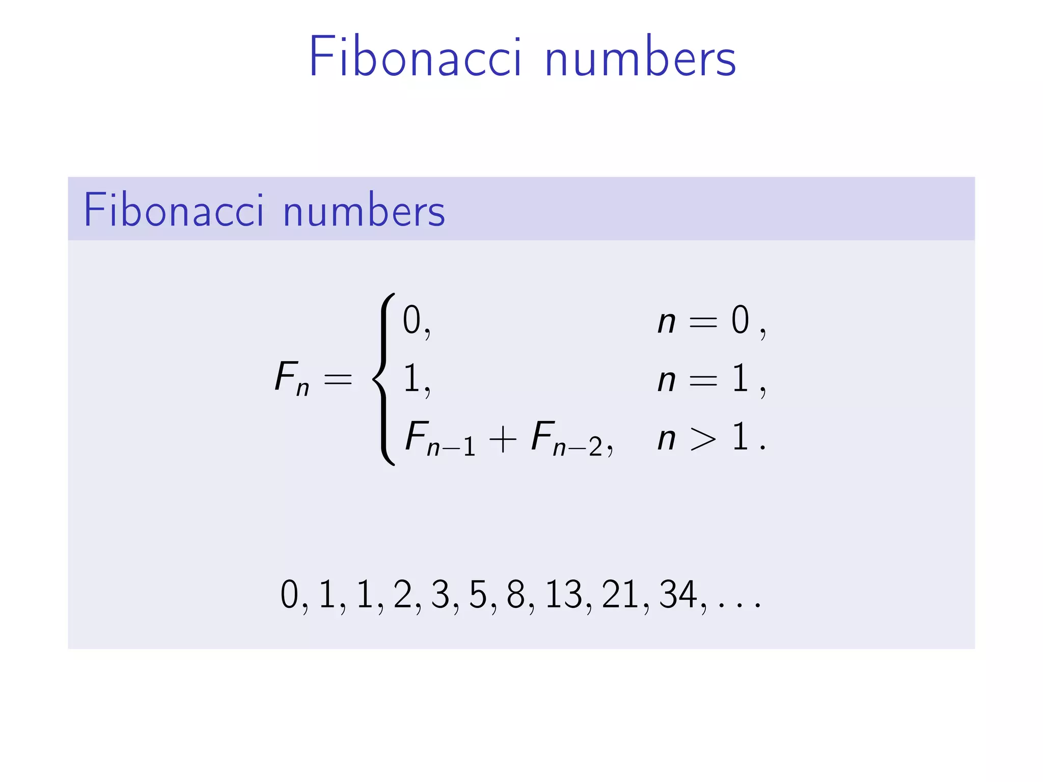
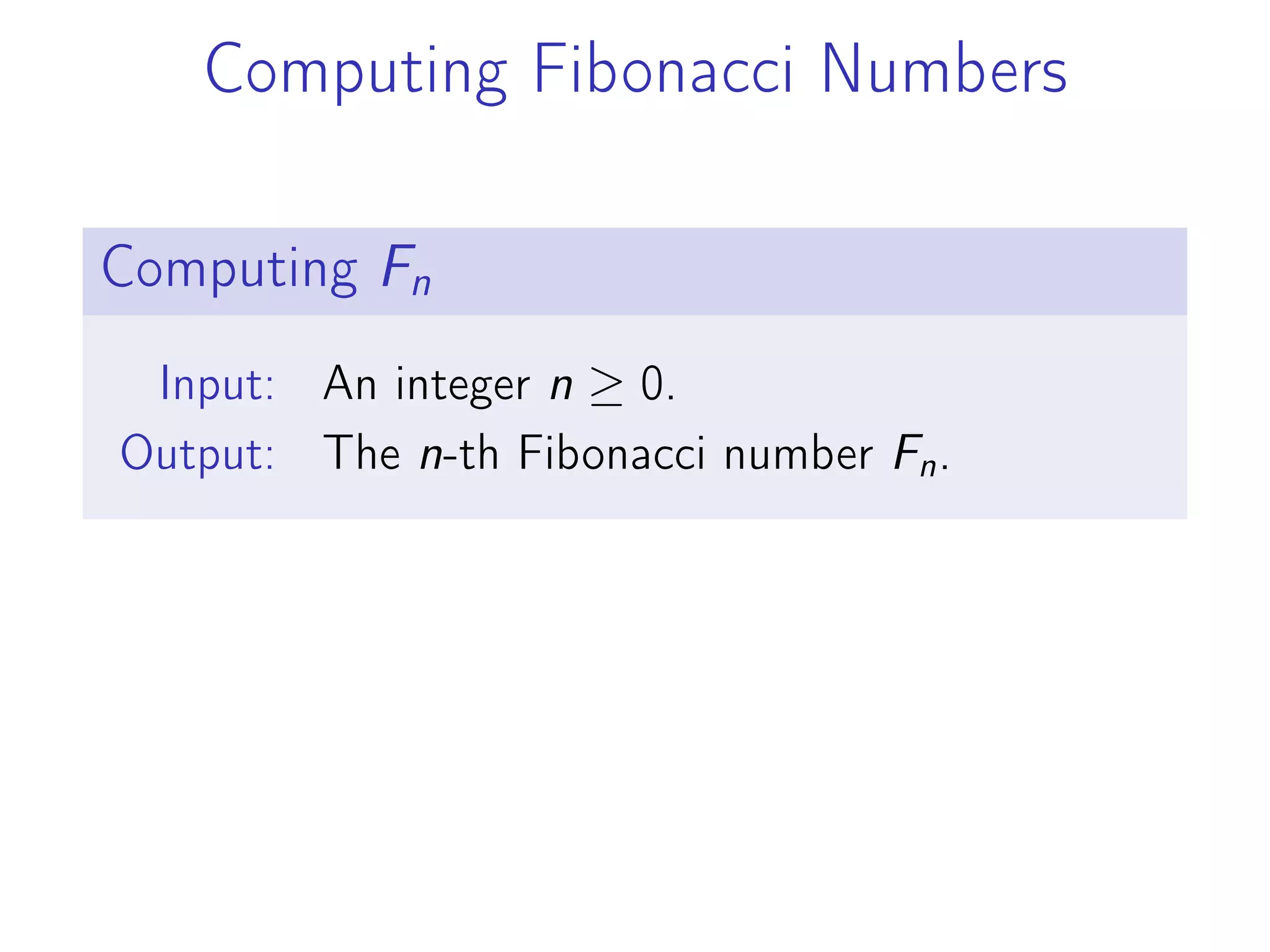
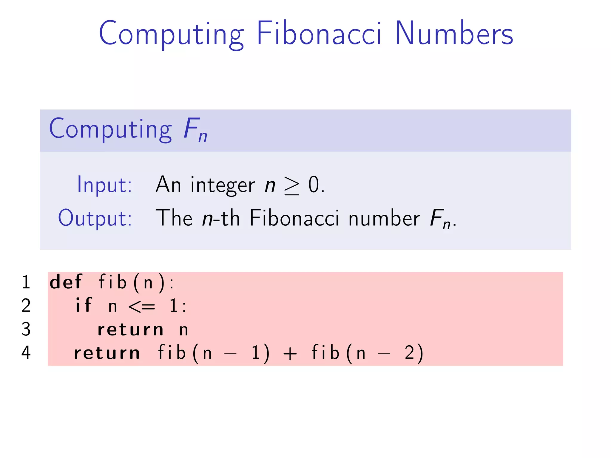
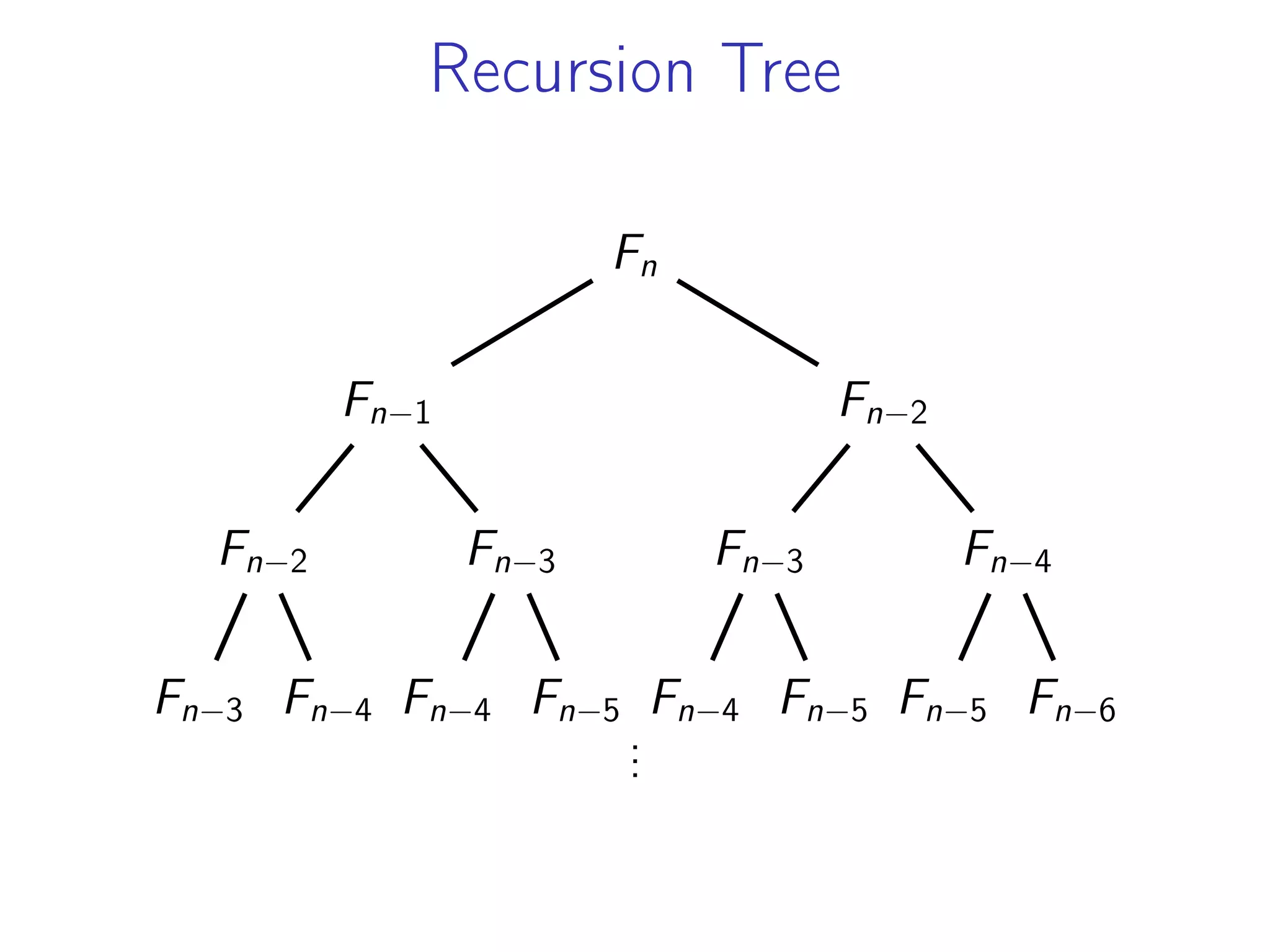
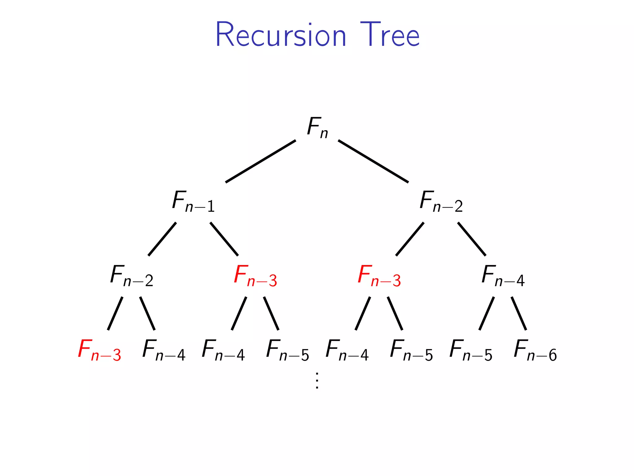
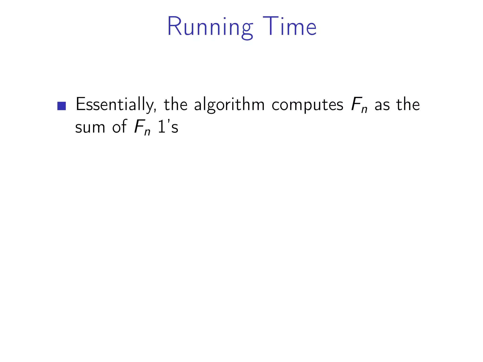
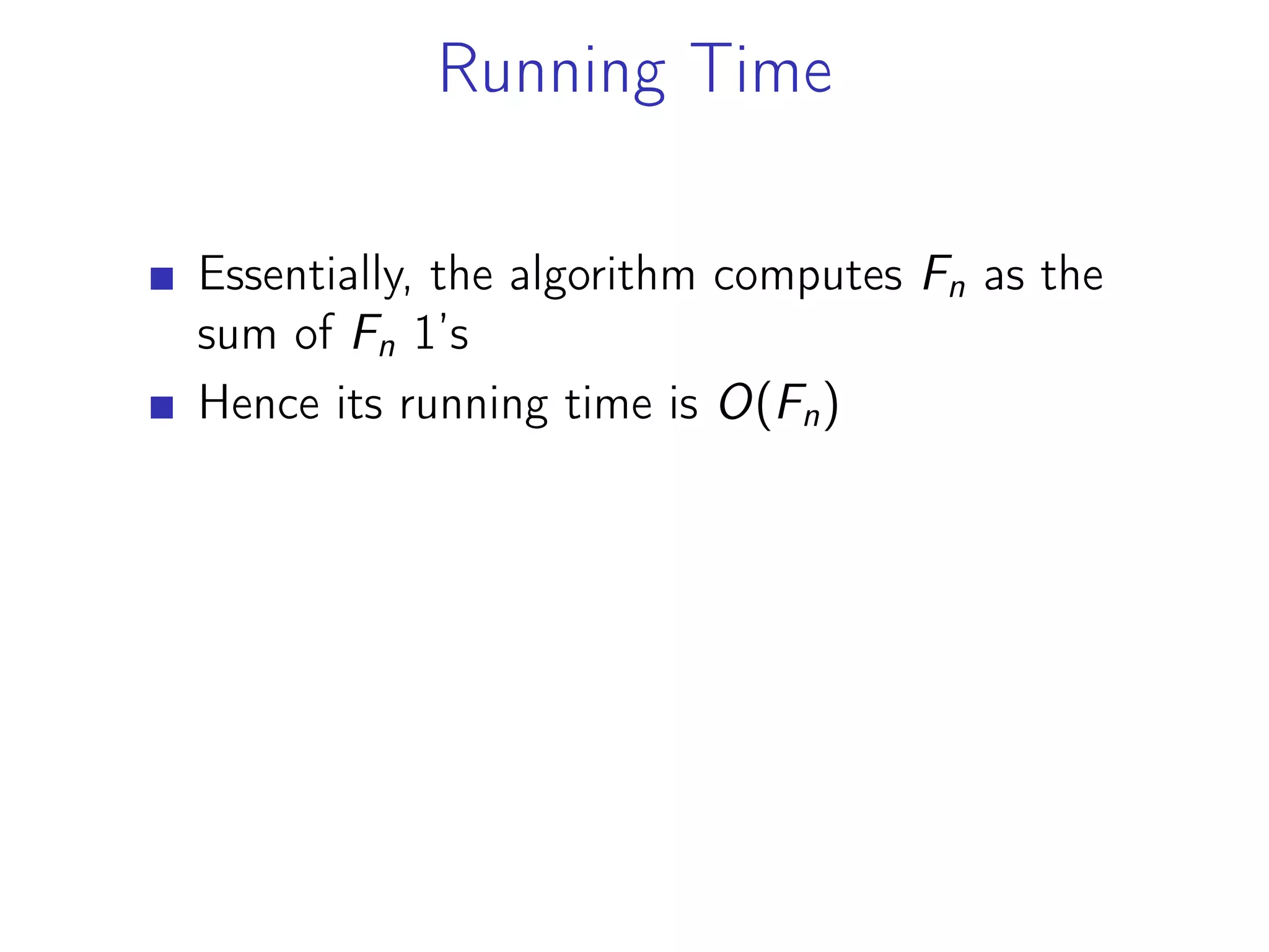
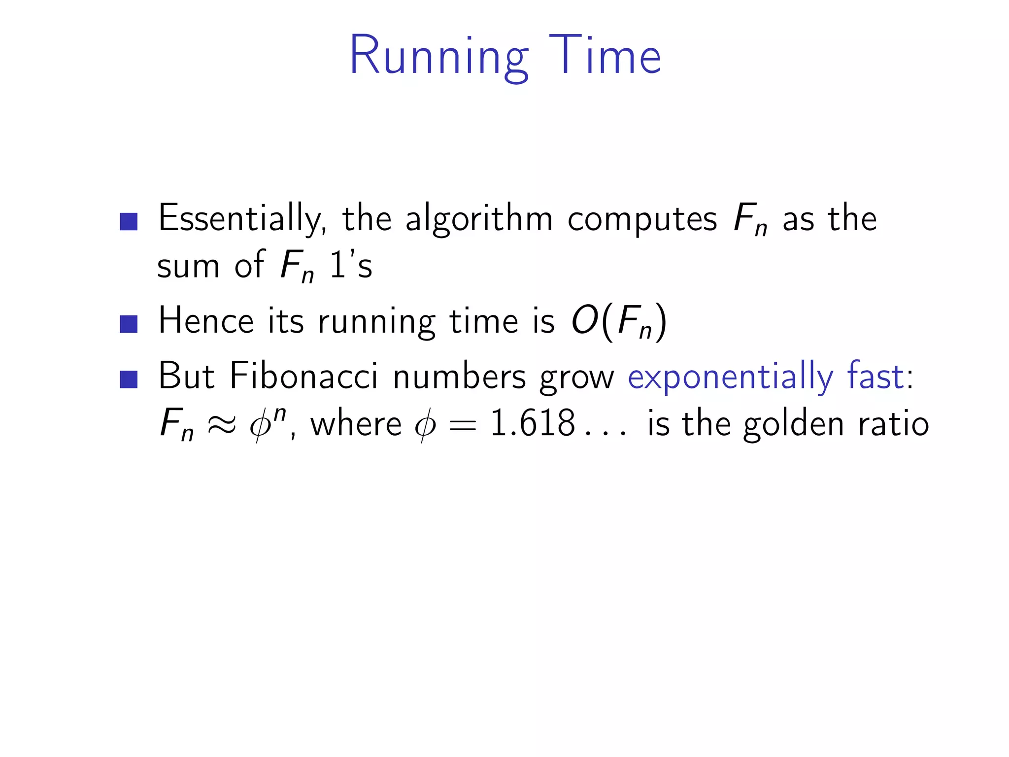
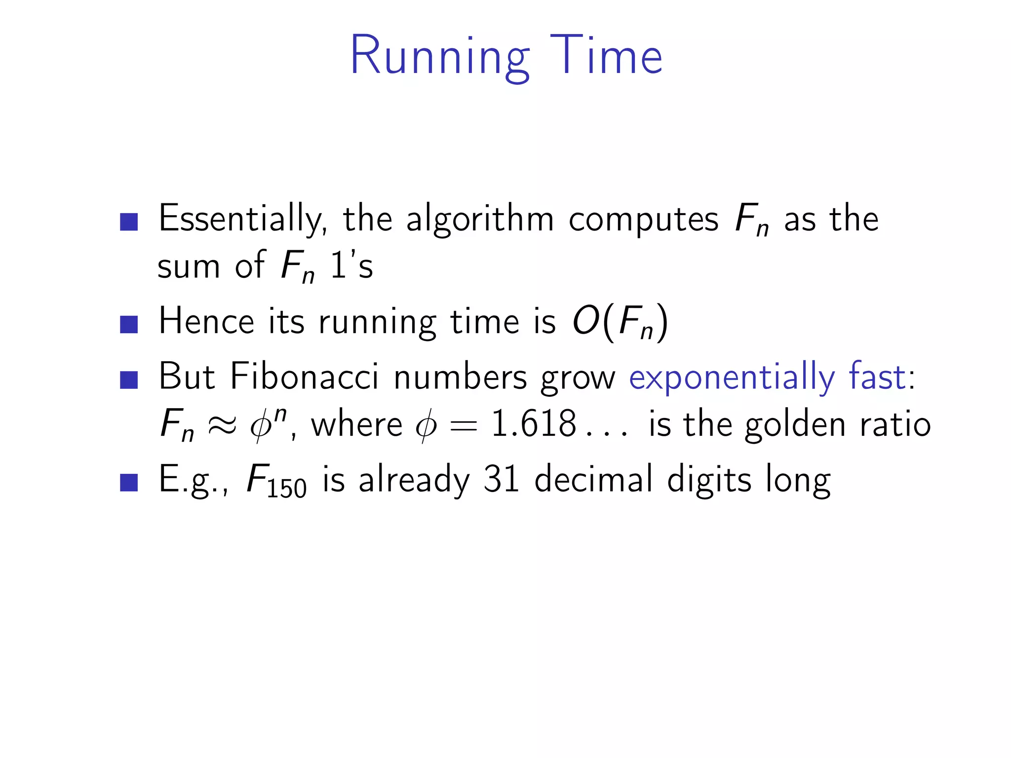
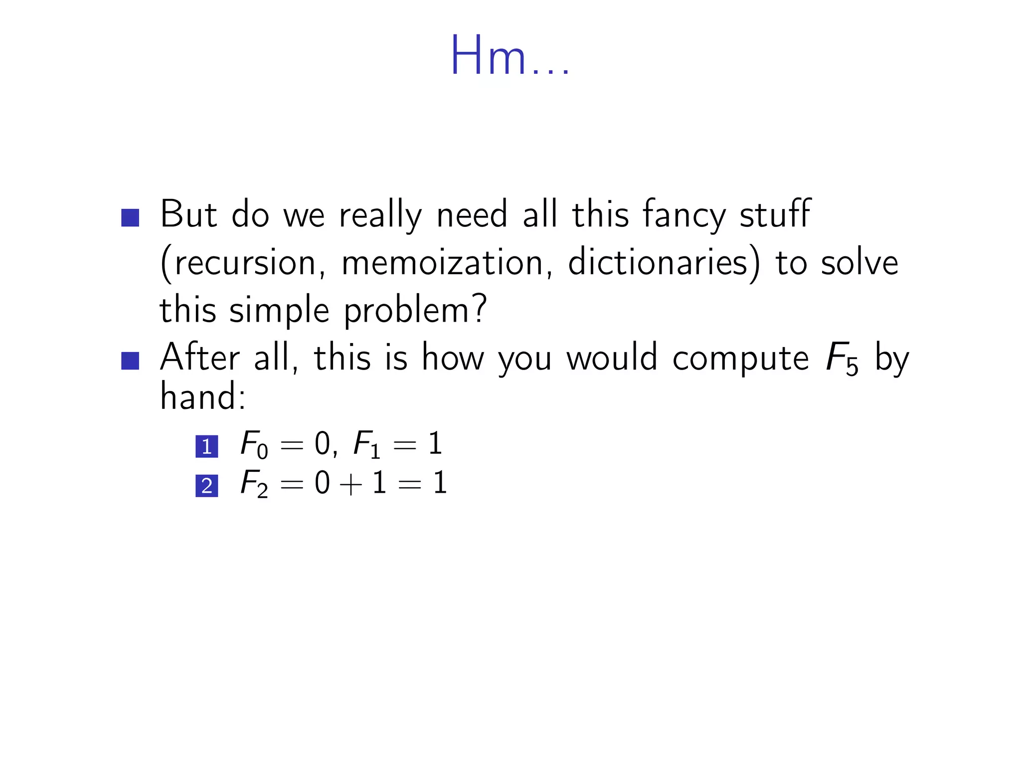
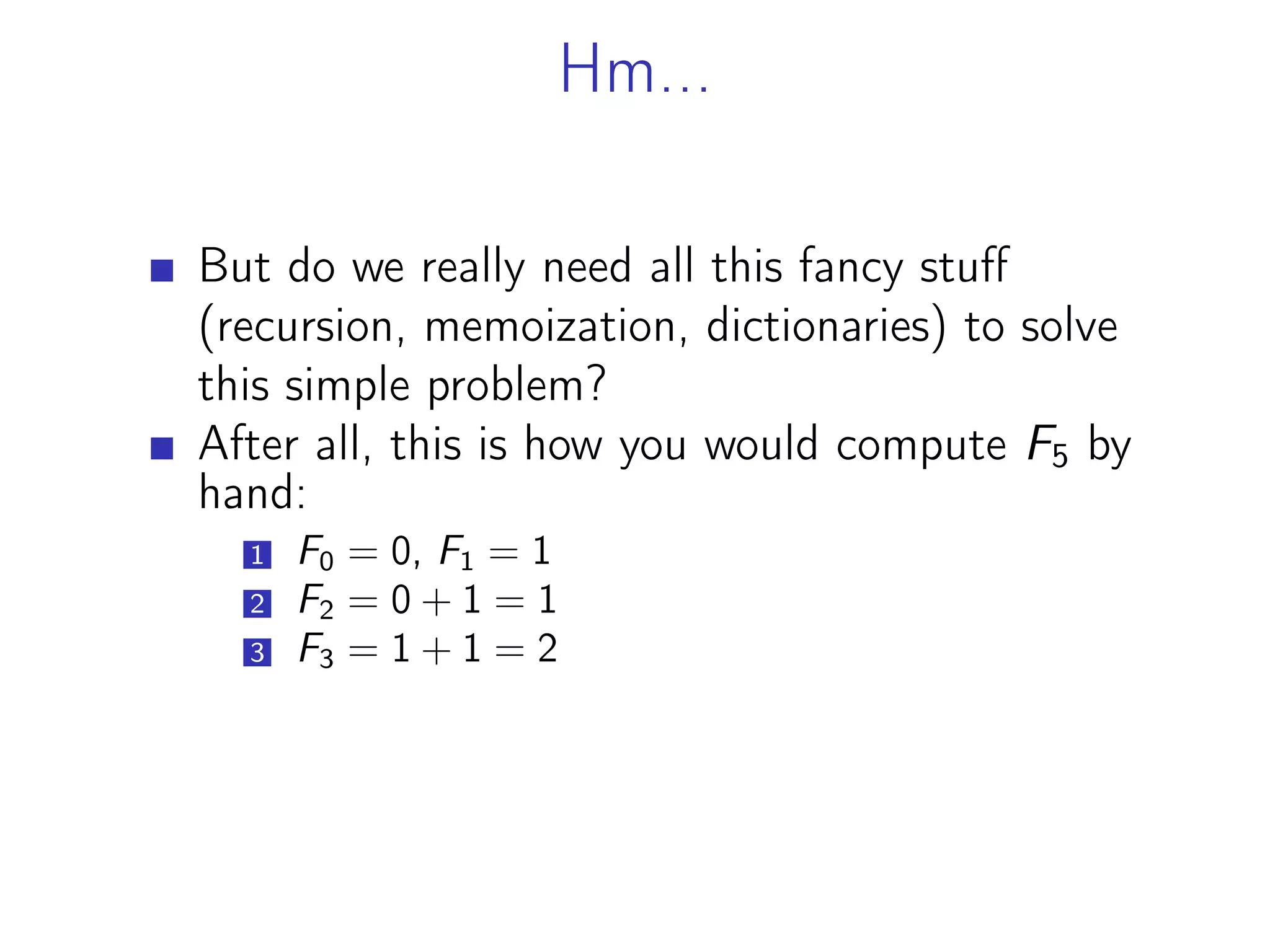
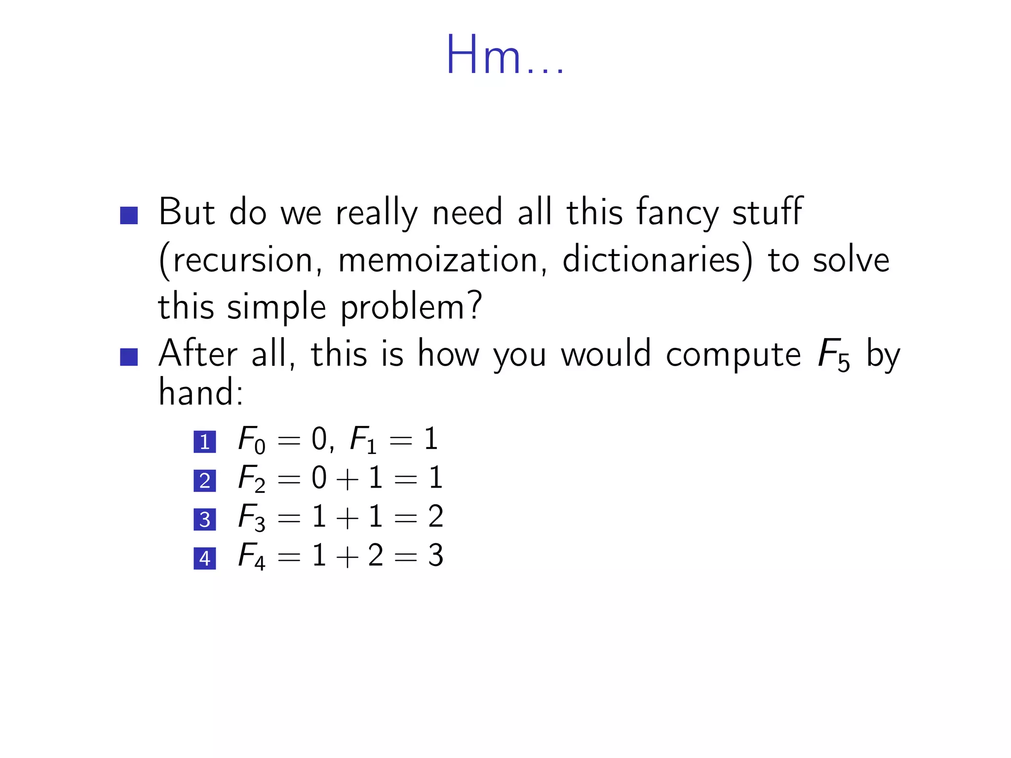
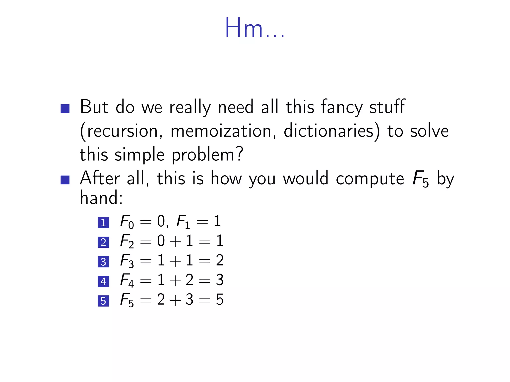
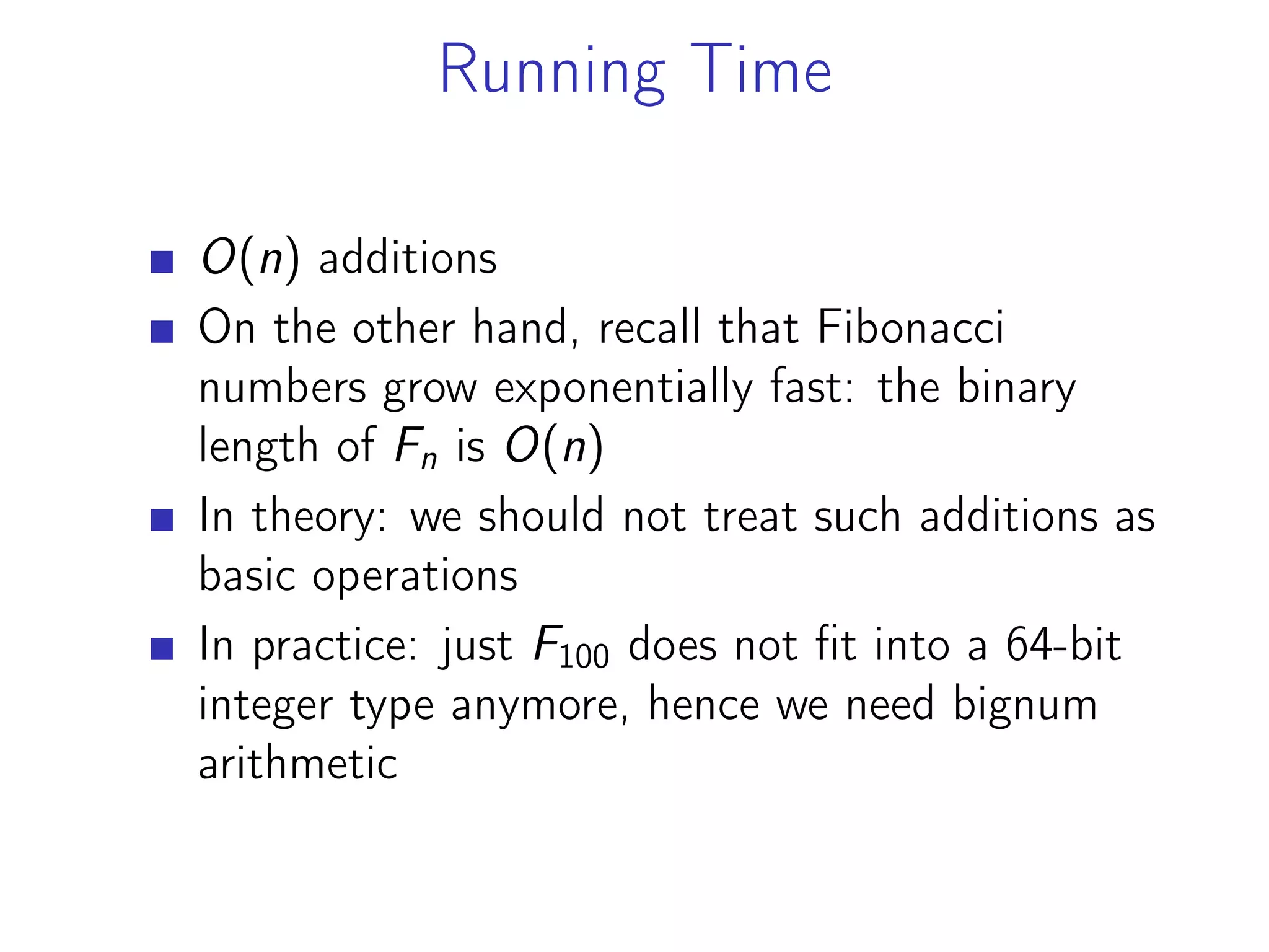
The document discusses the technique of dynamic programming. It begins with an example of using dynamic programming to compute the Fibonacci numbers more efficiently than a naive recursive solution. This involves storing previously computed values in a table to avoid recomputing them. The document then presents the problem of finding the longest increasing subsequence in an array. It defines the problem and subproblems, derives a recurrence relation, and provides both recursive and iterative memoized algorithms to solve it in quadratic time using dynamic programming.

![Memoization
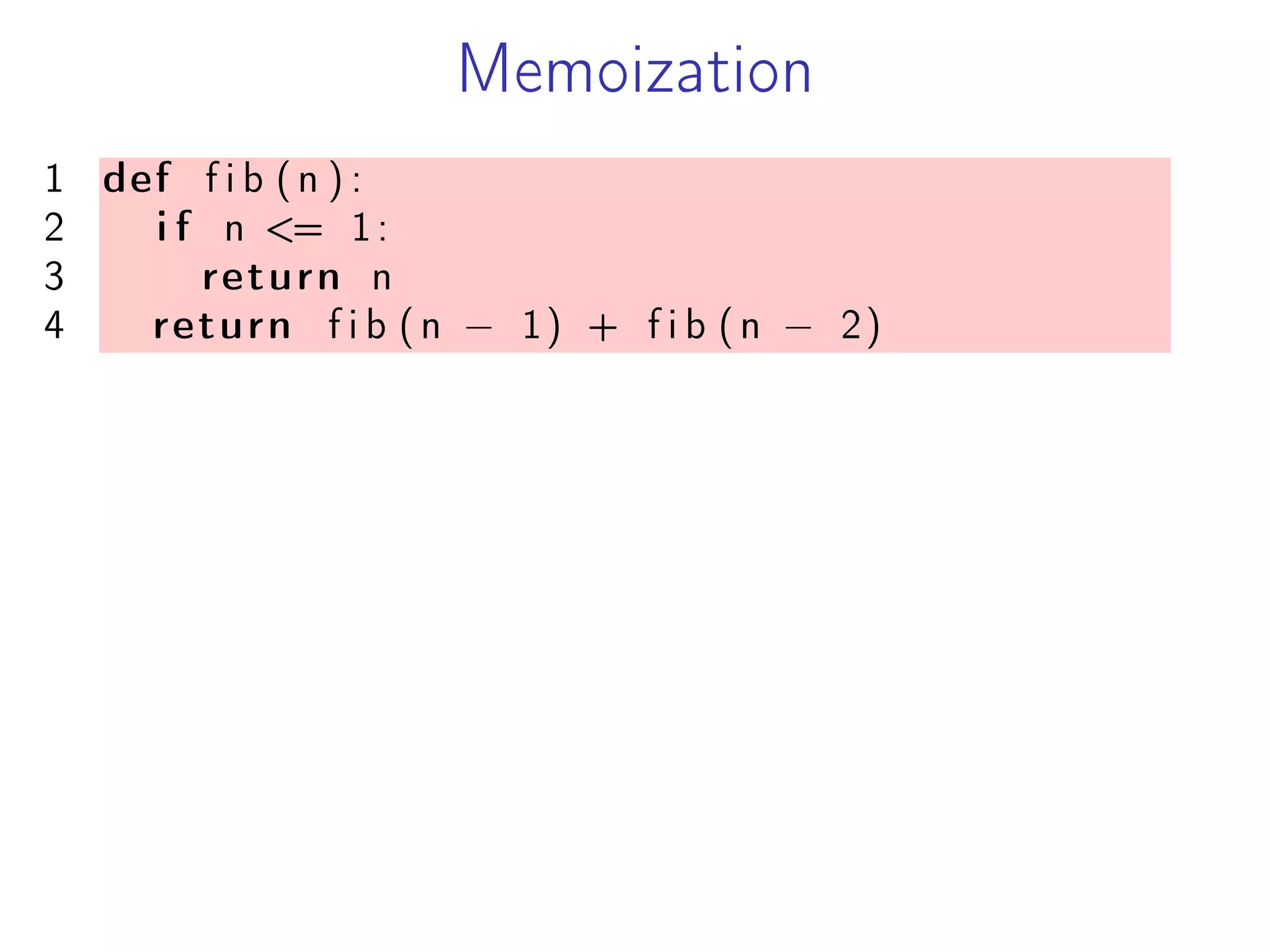
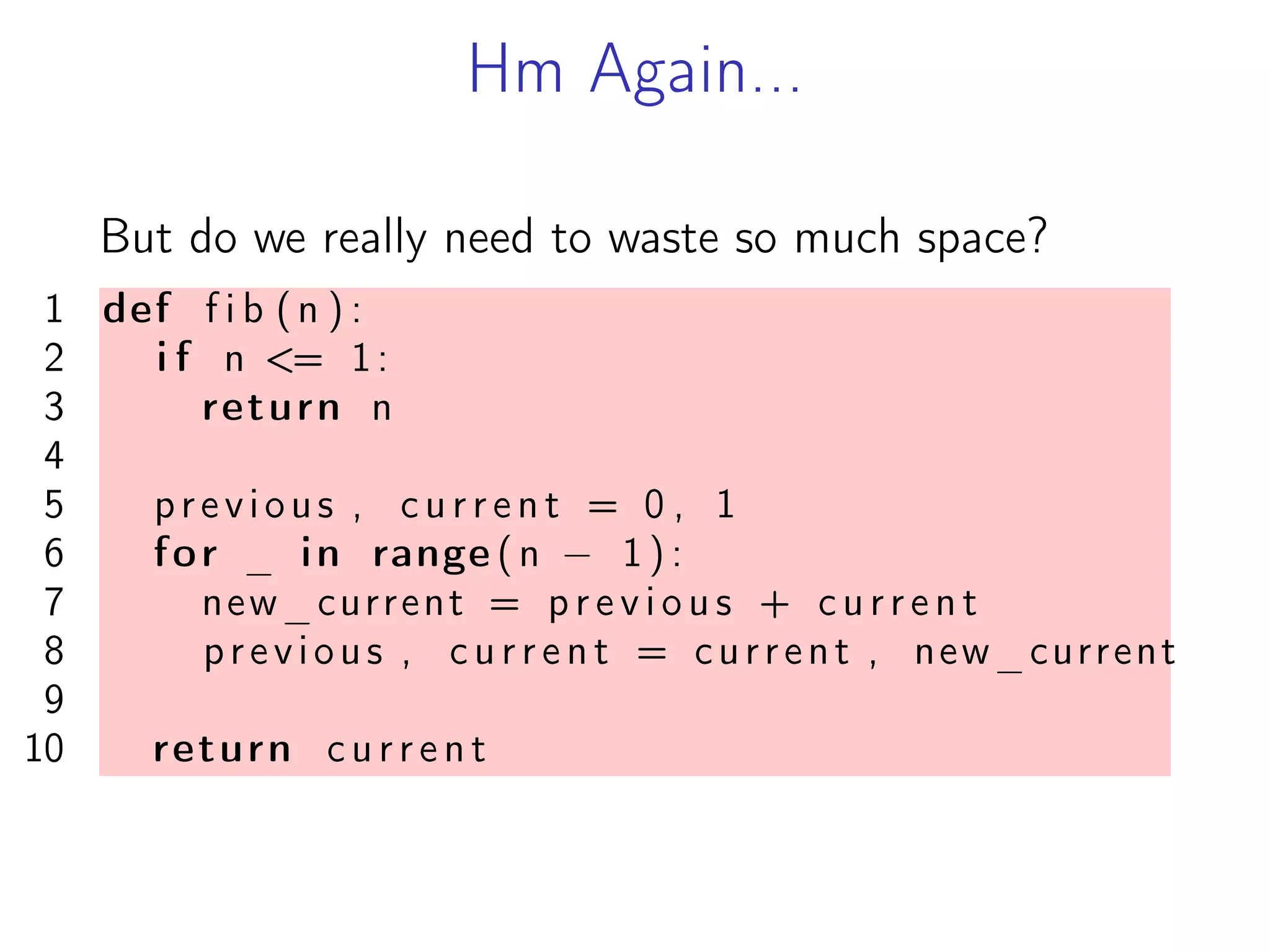
1 def f i b (n ) :
2 i f n <= 1:
3 return n
4 return f i b (n − 1) + f i b (n − 2)
1 T = dict()
2
3 def f i b (n ) :
4 if n not in T:
5 i f n <= 1:
6 T[n] = n
7 else :
8 T[n] = f i b (n − 1) + f i b (n − 2)
9
10 return T[n]](https://image.slidesharecdn.com/dynamicprograming-220116082321/75/Dynamic-programing-21-2048.jpg)
![Iterative Algorithm
1 def f i b (n ) :
2 T = [ None ] * (n + 1)
3 T[ 0 ] , T[ 1 ] = 0 , 1
4
5 for i in range (2 , n + 1 ) :
6 T[ i ] = T[ i − 1] + T[ i − 2]
7
8 return T[ n ]](https://image.slidesharecdn.com/dynamicprograming-220116082321/75/Dynamic-programing-29-2048.jpg)

![Longest Increasing Subsequence
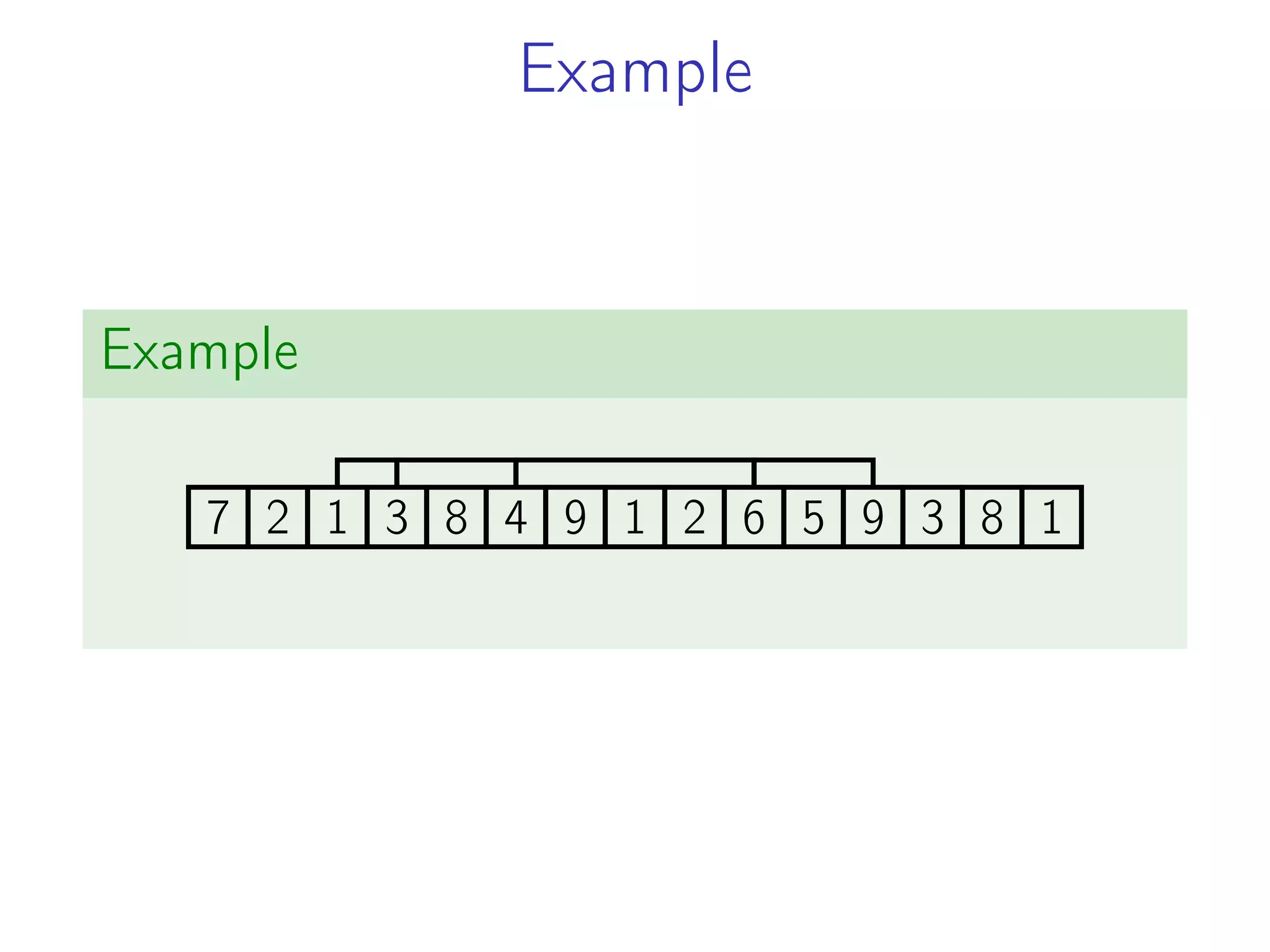
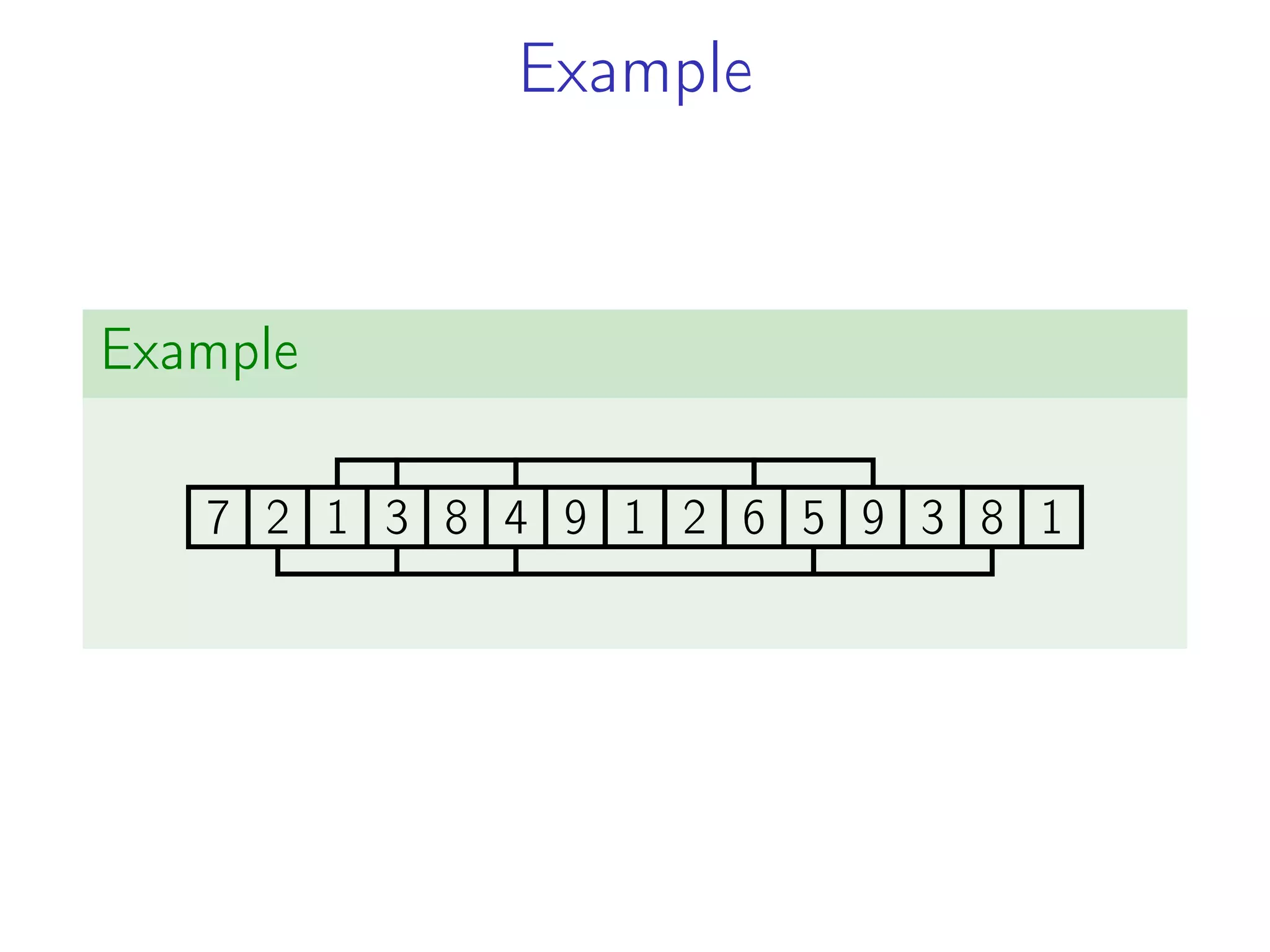
Longest increasing subsequence
Input: An array A = [a0, a1, . . . , an−1].
Output: A longest increasing subsequence (LIS),
i.e., ai1
, ai2
, . . . , aik
such that
i1 < i2 < . . . < ik, ai1
< ai2
< · · · < aik
,
and k is maximal.](https://image.slidesharecdn.com/dynamicprograming-220116082321/75/Dynamic-programing-39-2048.jpg)
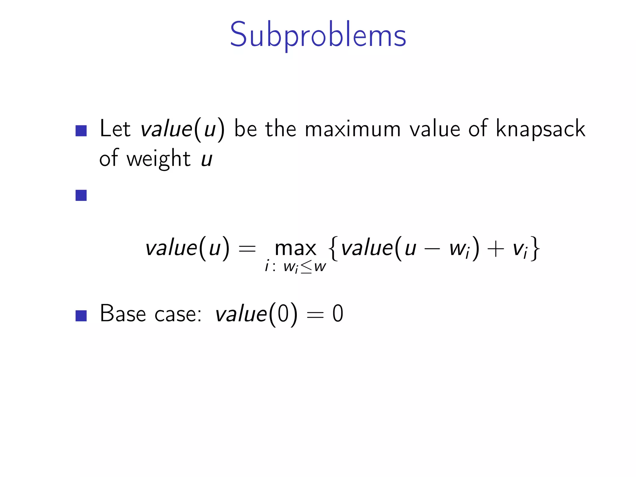
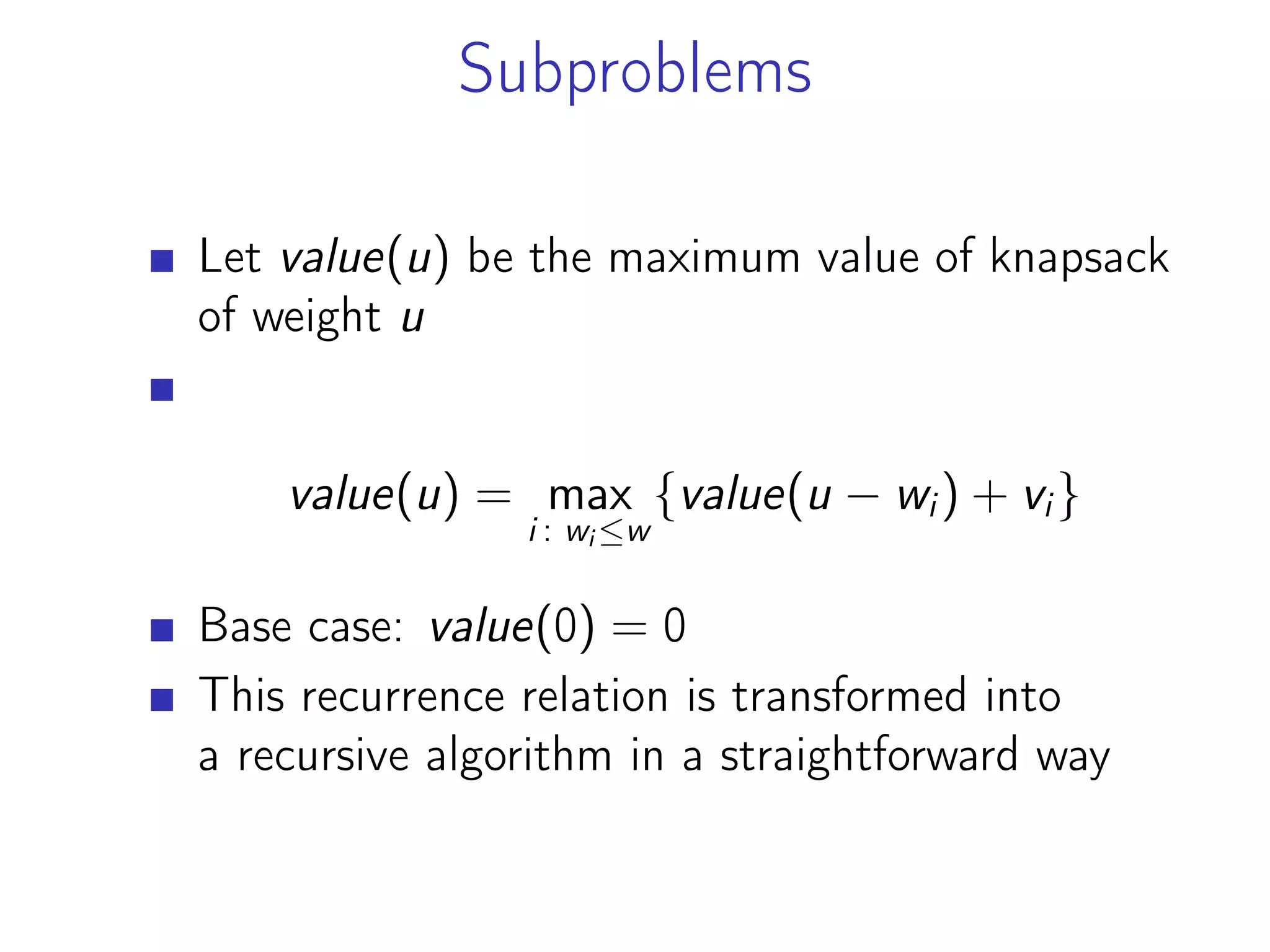
![Subproblems and Recurrence Relation
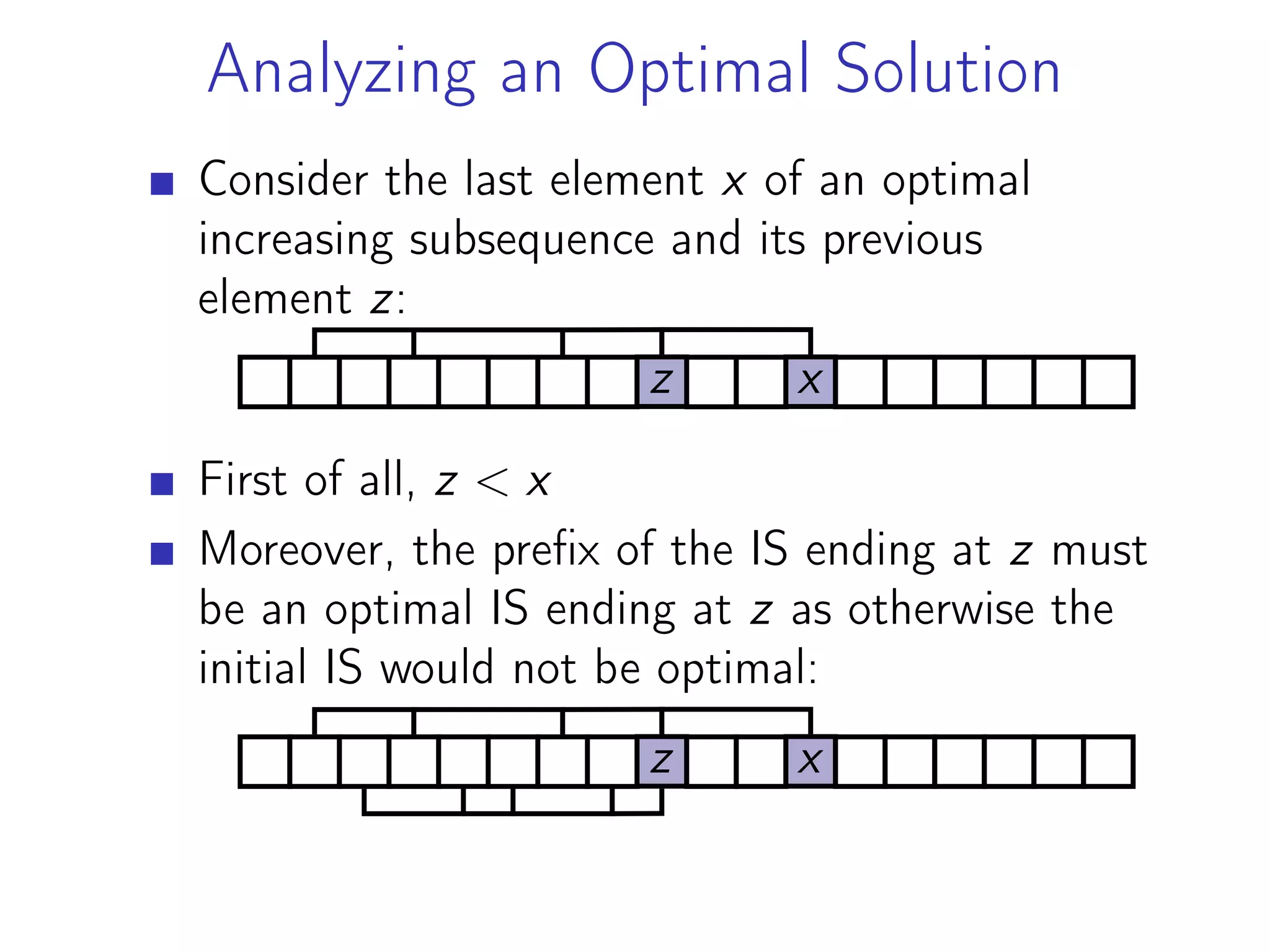
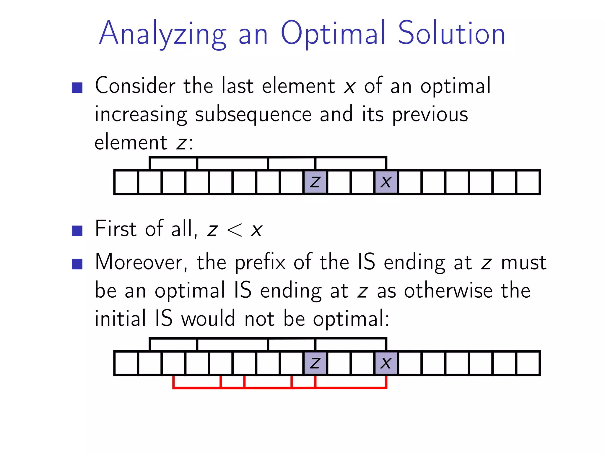
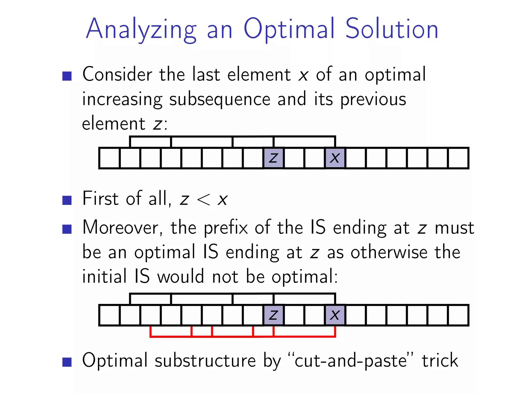
Let LIS(i) be the optimal length of a LIS ending
at A[i]](https://image.slidesharecdn.com/dynamicprograming-220116082321/75/Dynamic-programing-47-2048.jpg)
![Subproblems and Recurrence Relation
Let LIS(i) be the optimal length of a LIS ending
at A[i]
Then
LIS(i) = 1+max{LIS(j): j < i and A[j] < A[i]}](https://image.slidesharecdn.com/dynamicprograming-220116082321/75/Dynamic-programing-48-2048.jpg)
![Subproblems and Recurrence Relation
Let LIS(i) be the optimal length of a LIS ending
at A[i]
Then
LIS(i) = 1+max{LIS(j): j < i and A[j] < A[i]}
Convention: maximum of an empty set is equal
to zero](https://image.slidesharecdn.com/dynamicprograming-220116082321/75/Dynamic-programing-49-2048.jpg)
![Subproblems and Recurrence Relation
Let LIS(i) be the optimal length of a LIS ending
at A[i]
Then
LIS(i) = 1+max{LIS(j): j < i and A[j] < A[i]}
Convention: maximum of an empty set is equal
to zero
Base case: LIS(0) = 1](https://image.slidesharecdn.com/dynamicprograming-220116082321/75/Dynamic-programing-50-2048.jpg)
![Algorithm
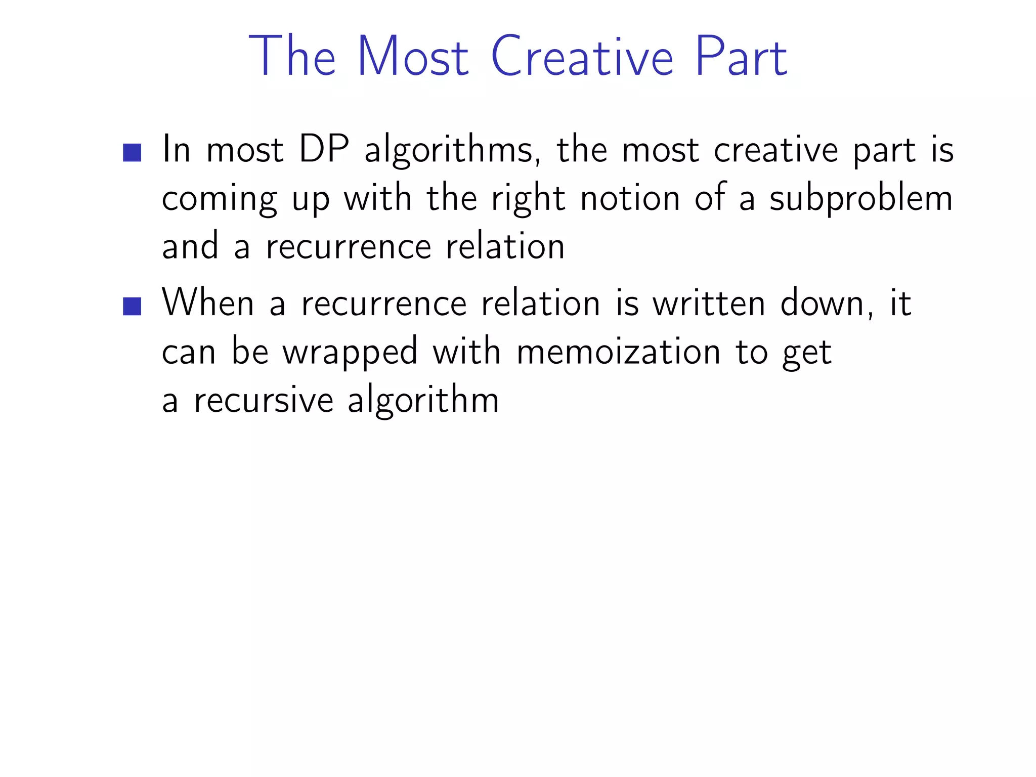
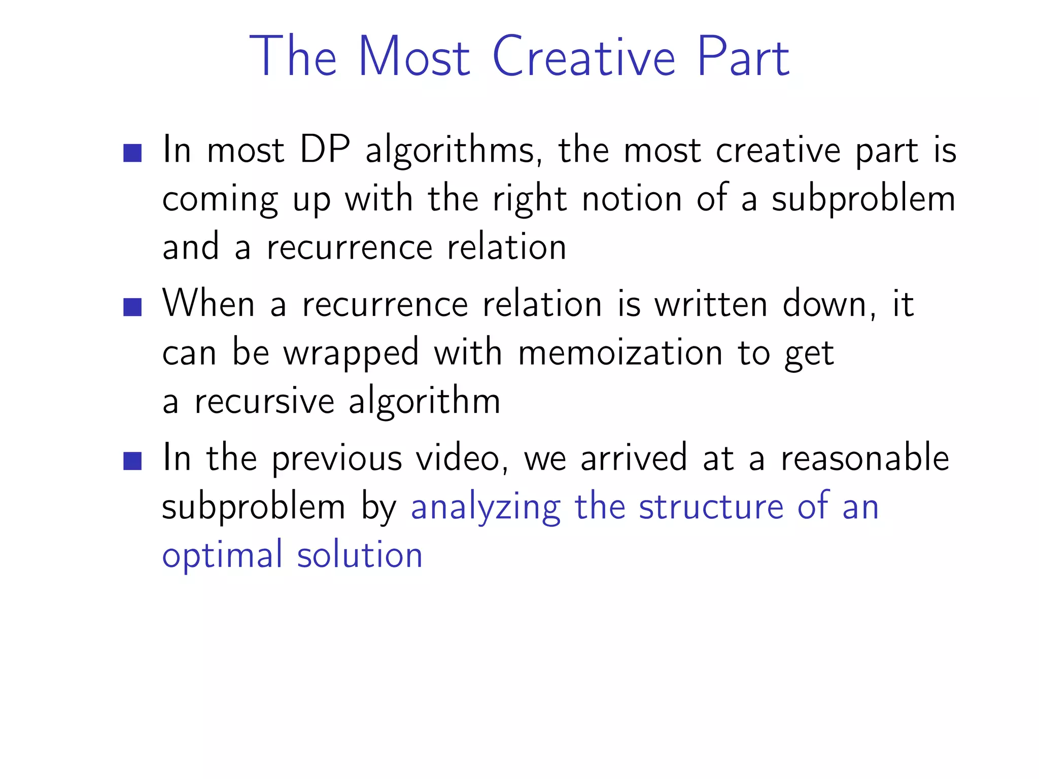
When we have a recurrence relation at hand,
converting it to a recursive algorithm with
memoization is just a technicality
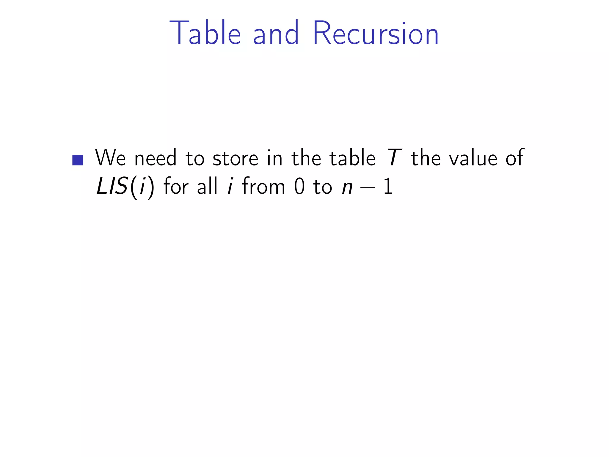
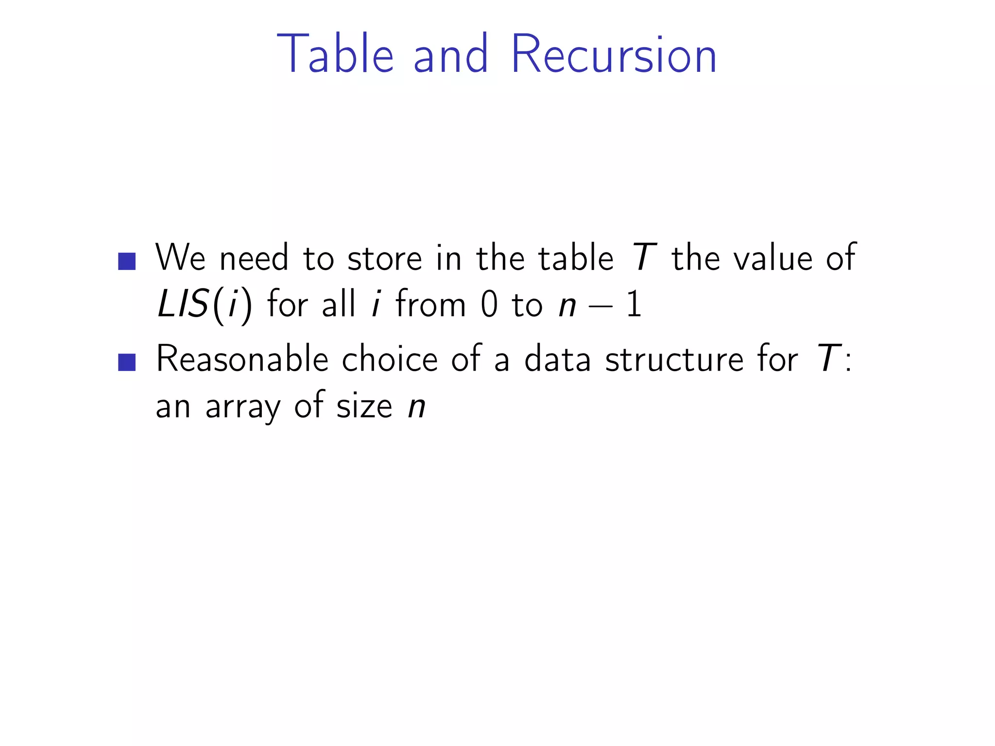
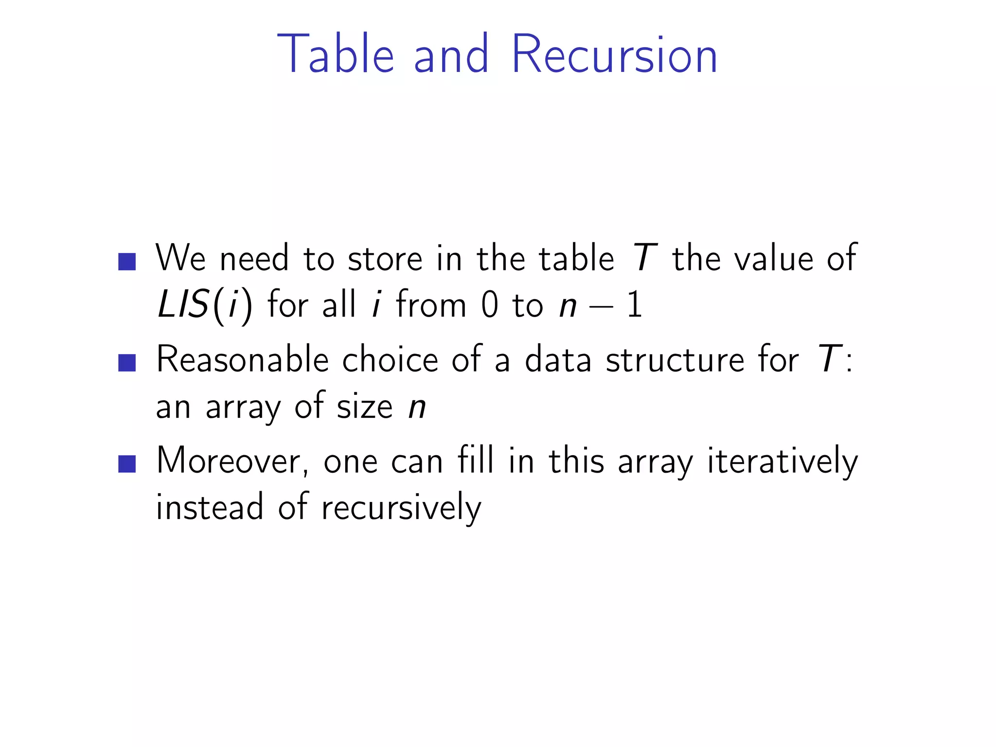
We will use a table T to store the results:
T[i] = LIS(i)](https://image.slidesharecdn.com/dynamicprograming-220116082321/75/Dynamic-programing-51-2048.jpg)
![Algorithm
When we have a recurrence relation at hand,
converting it to a recursive algorithm with
memoization is just a technicality
We will use a table T to store the results:
T[i] = LIS(i)
Initially, T is empty. When LIS(i) is computed,
we store its value at T[i] (so that we will never
recompute LIS(i) again)](https://image.slidesharecdn.com/dynamicprograming-220116082321/75/Dynamic-programing-52-2048.jpg)
![Algorithm
When we have a recurrence relation at hand,
converting it to a recursive algorithm with
memoization is just a technicality
We will use a table T to store the results:
T[i] = LIS(i)
Initially, T is empty. When LIS(i) is computed,
we store its value at T[i] (so that we will never
recompute LIS(i) again)
The exact data structure behind T is not that
important at this point: it could be an array or
a hash table](https://image.slidesharecdn.com/dynamicprograming-220116082321/75/Dynamic-programing-53-2048.jpg)
![Memoization
1 T = dict ()
2
3 def l i s (A, i ) :
4 i f i not in T:
5 T[ i ] = 1
6
7 for j in range ( i ) :
8 i f A[ j ] < A[ i ] :
9 T[ i ] = max(T[ i ] , l i s (A, j ) + 1)
10
11 return T[ i ]
12
13 A = [7 , 2 , 1 , 3 , 8 , 4 , 9 , 1 , 2 , 6 , 5 , 9 , 3]
14 print (max( l i s (A, i ) for i in range ( len (A) ) ) )](https://image.slidesharecdn.com/dynamicprograming-220116082321/75/Dynamic-programing-54-2048.jpg)
![Iterative Algorithm
1 def l i s (A) :
2 T = [ None ] * len (A)
3
4 for i in range ( len (A ) ) :
5 T[ i ] = 1
6 for j in range ( i ) :
7 i f A[ j ] < A[ i ] and T[ i ] < T[ j ] + 1:
8 T[ i ] = T[ j ] + 1
9
10 return max(T[ i ] for i in range ( len (A) ) )](https://image.slidesharecdn.com/dynamicprograming-220116082321/75/Dynamic-programing-59-2048.jpg)
![Iterative Algorithm
1 def l i s (A) :
2 T = [ None ] * len (A)
3
4 for i in range ( len (A ) ) :
5 T[ i ] = 1
6 for j in range ( i ) :
7 i f A[ j ] < A[ i ] and T[ i ] < T[ j ] + 1:
8 T[ i ] = T[ j ] + 1
9
10 return max(T[ i ] for i in range ( len (A) ) )
Crucial property: when computing T[i], T[j] for
all j < i have already been computed](https://image.slidesharecdn.com/dynamicprograming-220116082321/75/Dynamic-programing-60-2048.jpg)
![Iterative Algorithm
1 def l i s (A) :
2 T = [ None ] * len (A)
3
4 for i in range ( len (A ) ) :
5 T[ i ] = 1
6 for j in range ( i ) :
7 i f A[ j ] < A[ i ] and T[ i ] < T[ j ] + 1:
8 T[ i ] = T[ j ] + 1
9
10 return max(T[ i ] for i in range ( len (A) ) )
Crucial property: when computing T[i], T[j] for
all j < i have already been computed
Running time: O(n2
)](https://image.slidesharecdn.com/dynamicprograming-220116082321/75/Dynamic-programing-61-2048.jpg)
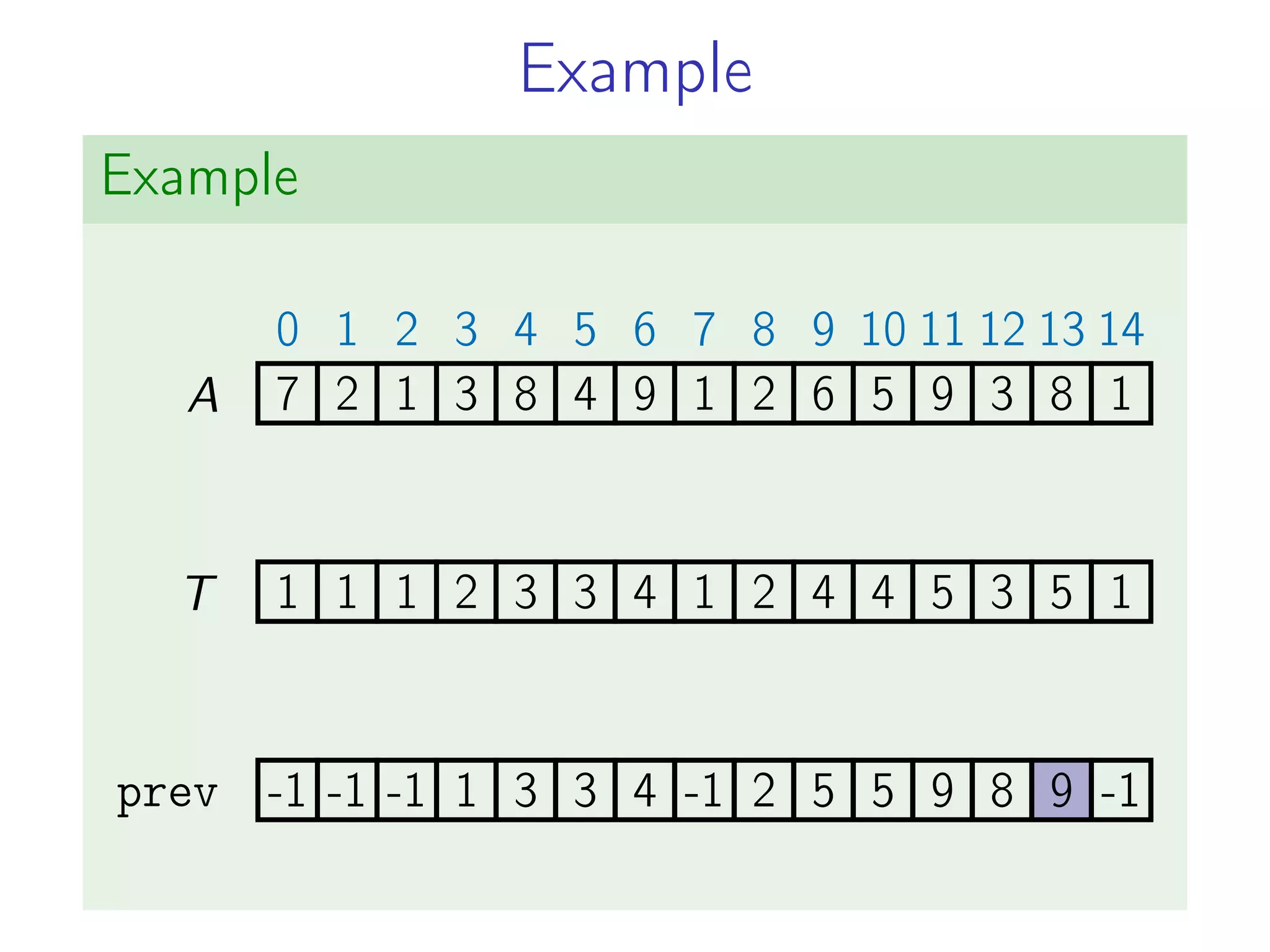
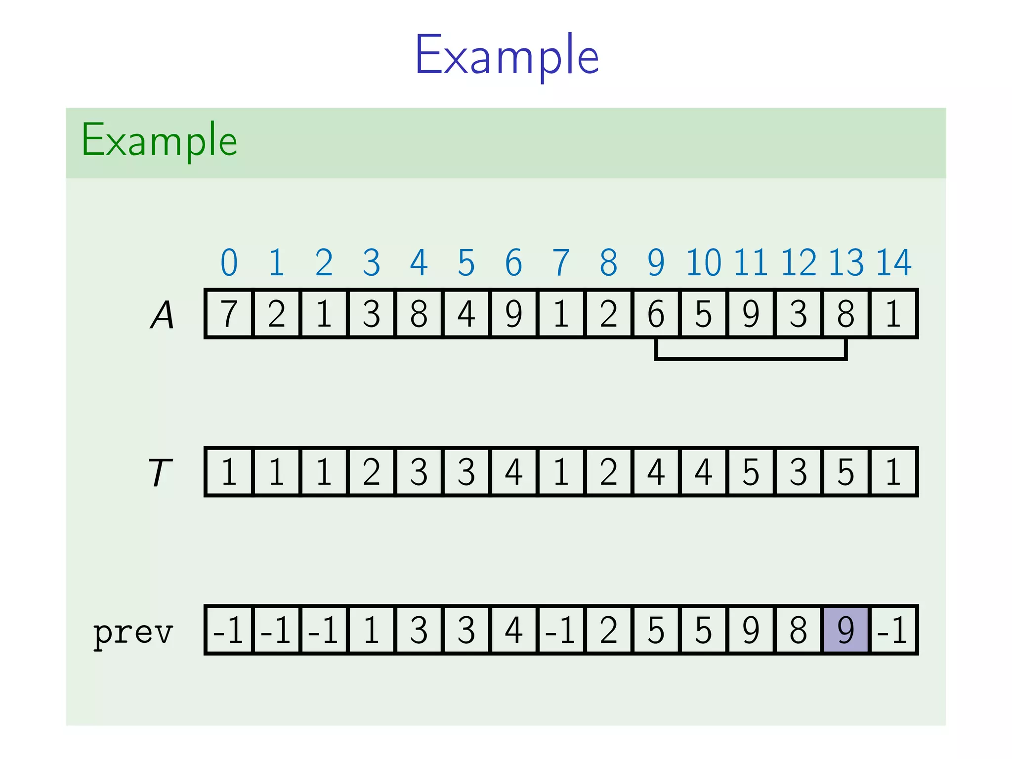
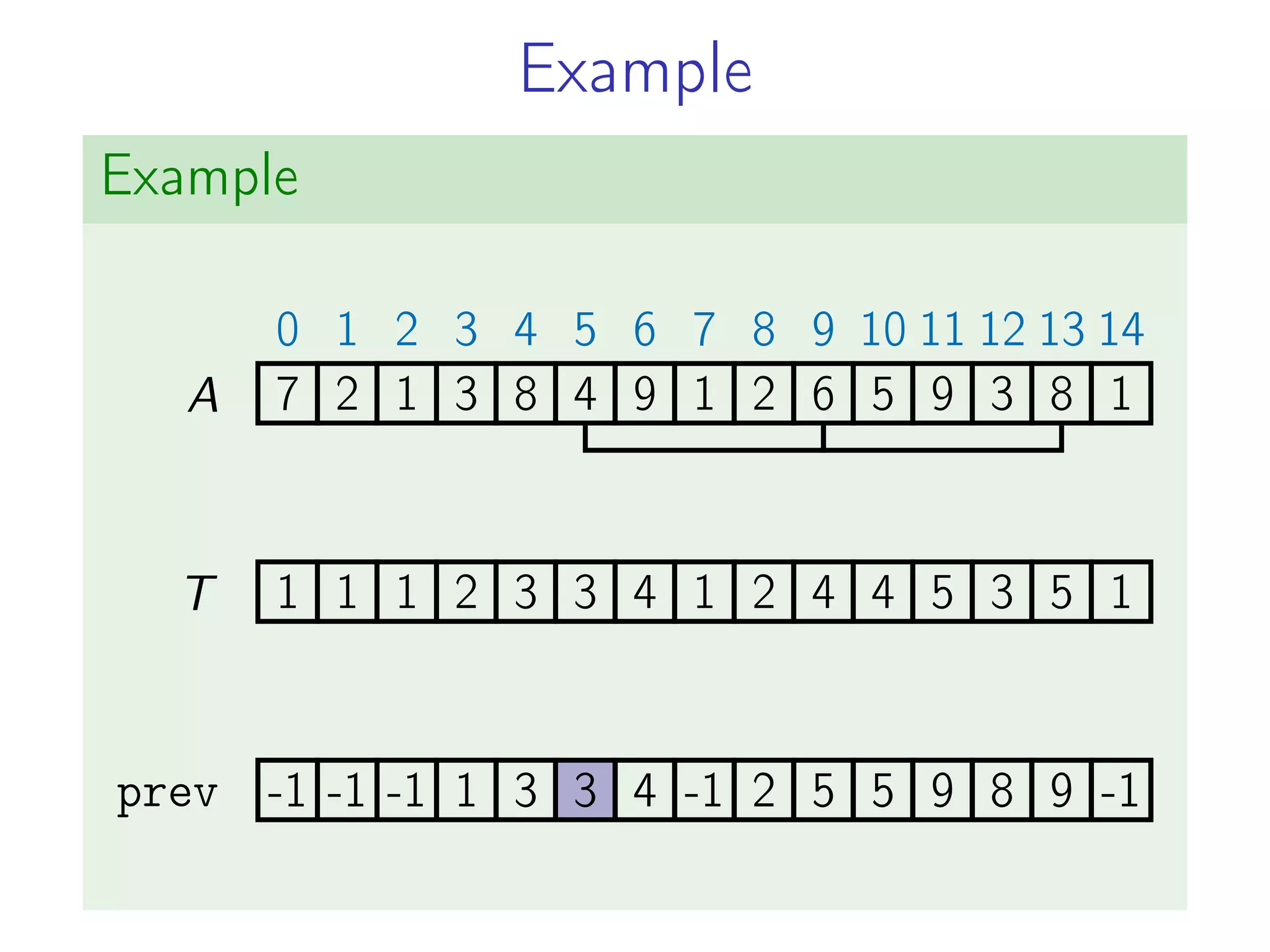
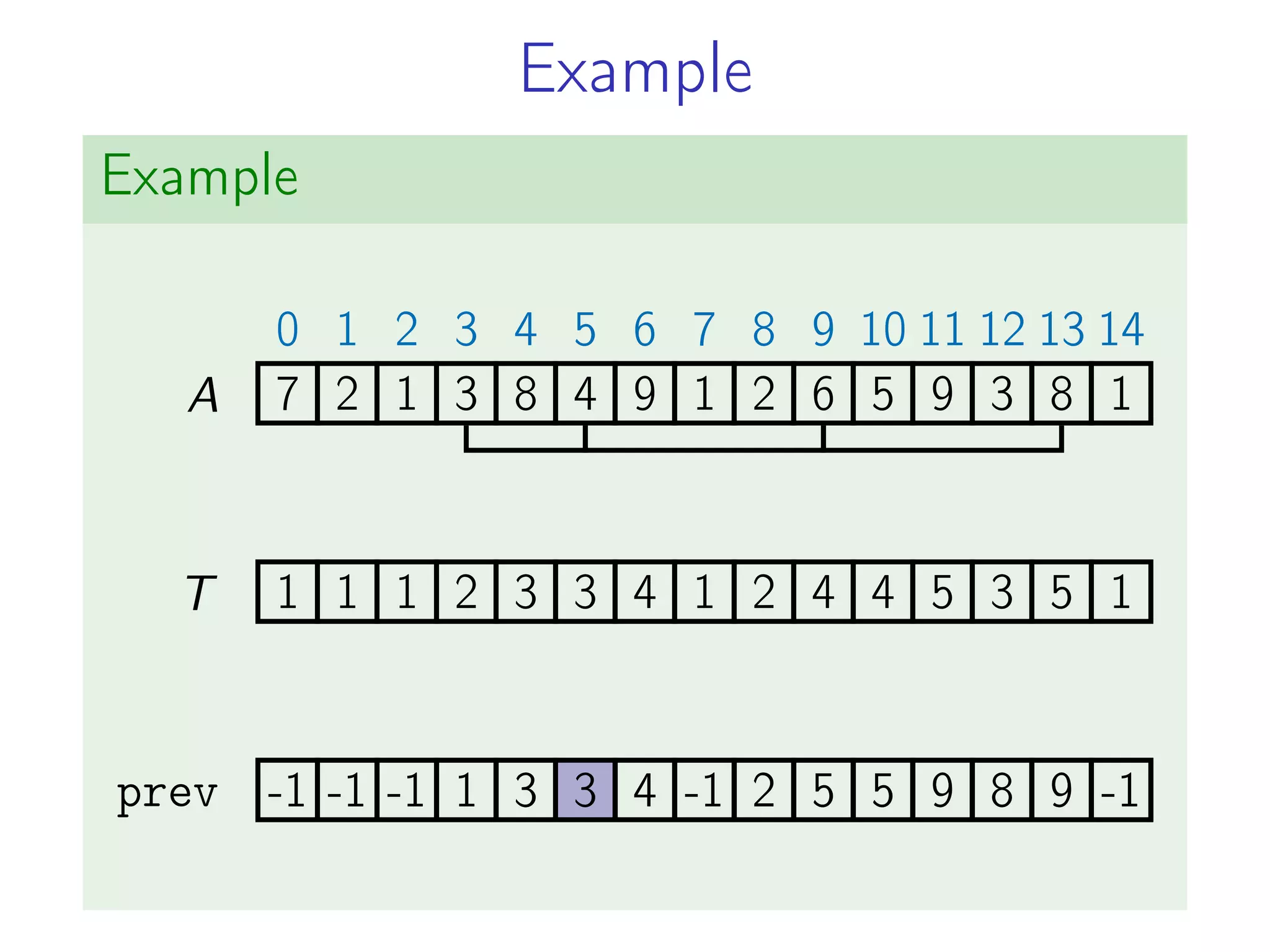
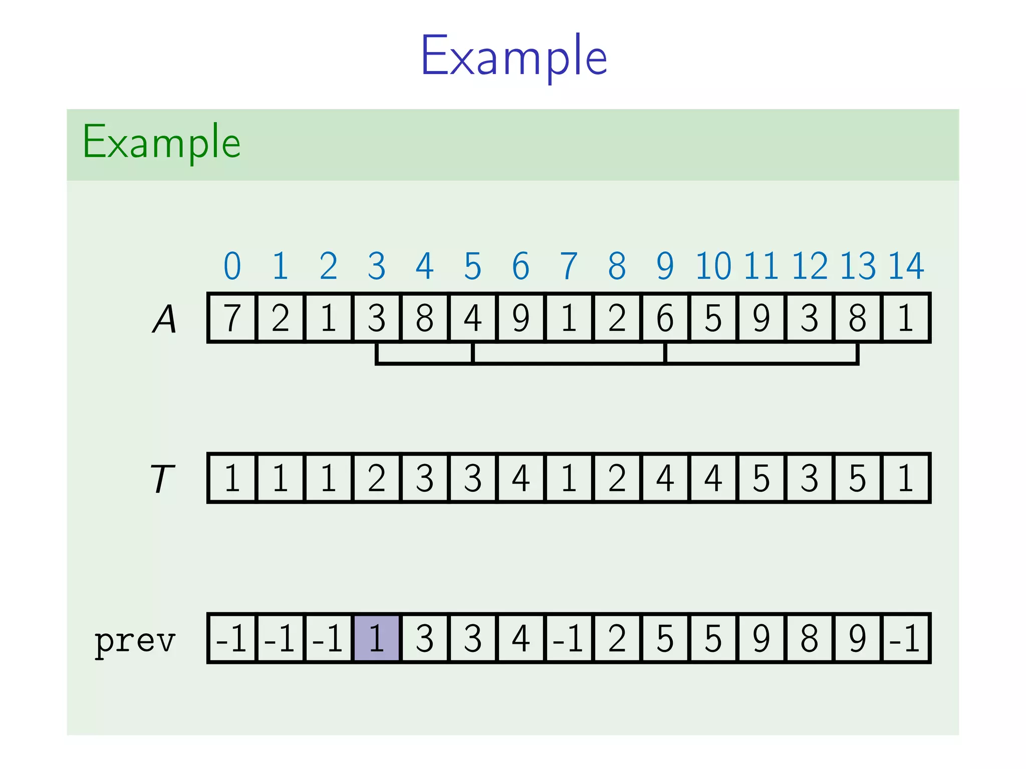
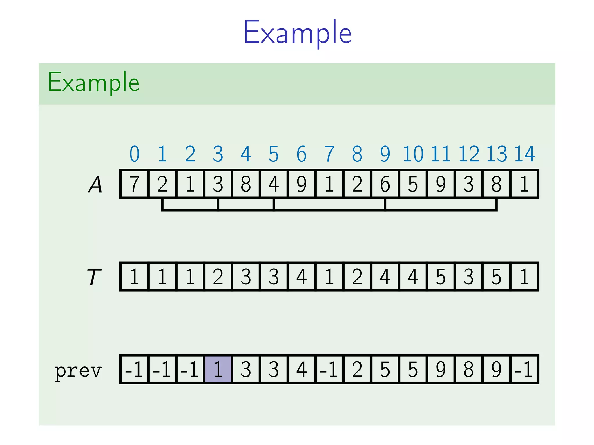
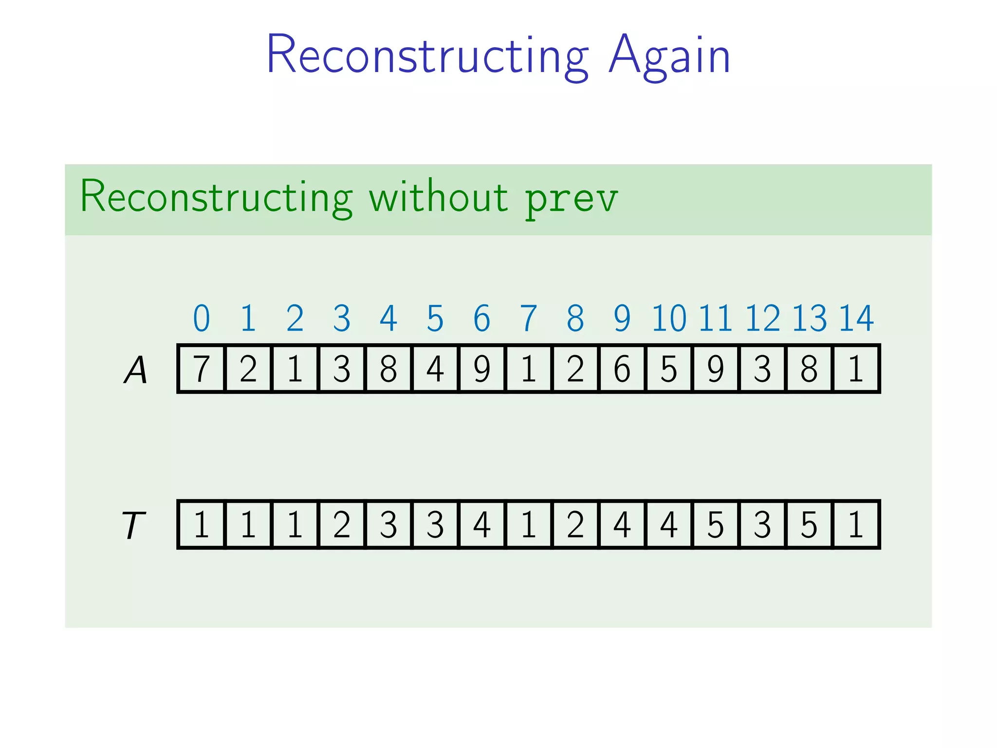
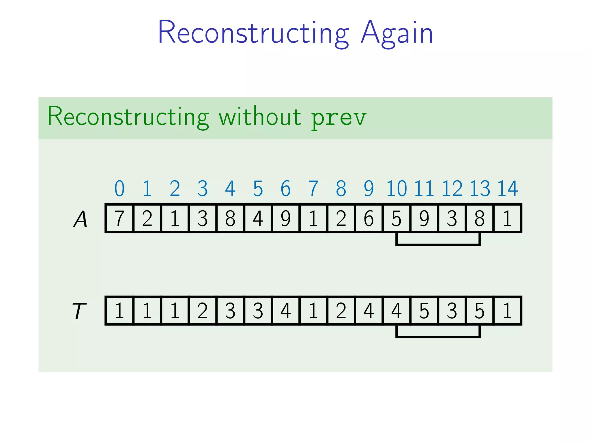
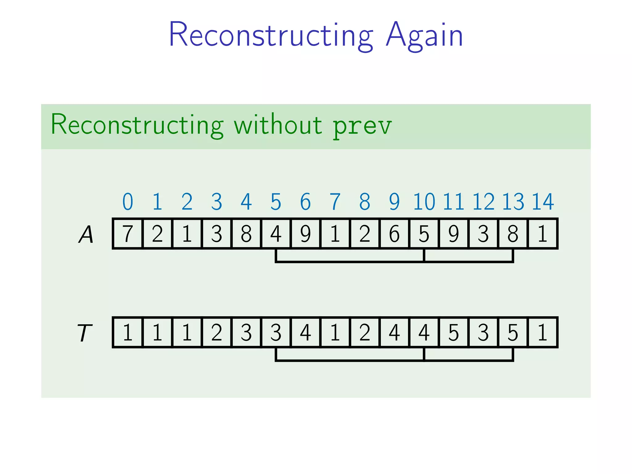
![Adjusting the Algorithm
1 def l i s (A) :
2 T = [ None ] * len (A)
3 prev = [None] * len(A)
4
5 for i in range ( len (A ) ) :
6 T[ i ] = 1
7 prev[i] = -1
8 for j in range ( i ) :
9 i f A[ j ] < A[ i ] and T[ i ] < T[ j ] + 1:
10 T[ i ] = T[ j ] + 1
11 prev[i] = j](https://image.slidesharecdn.com/dynamicprograming-220116082321/75/Dynamic-programing-65-2048.jpg)
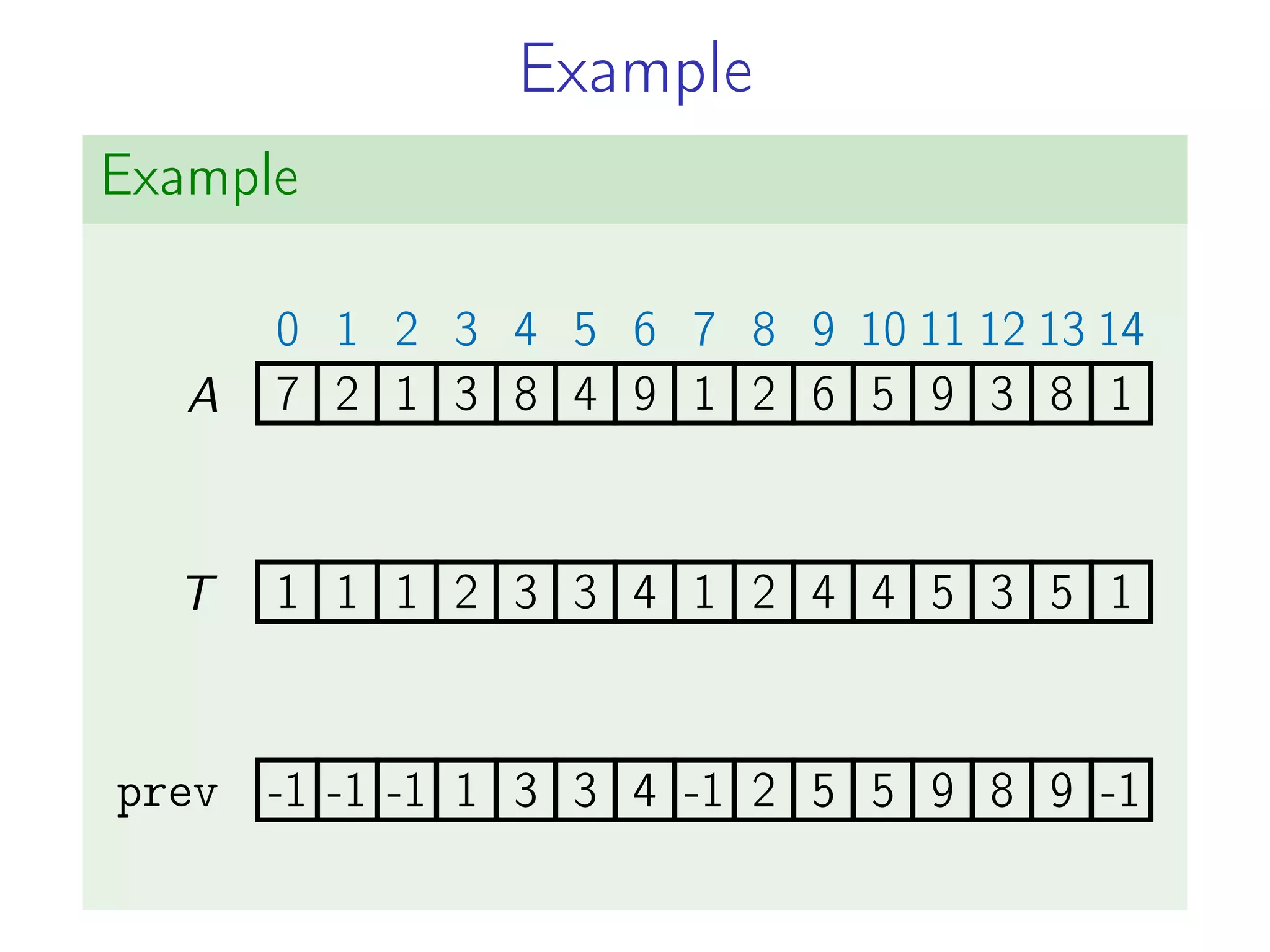
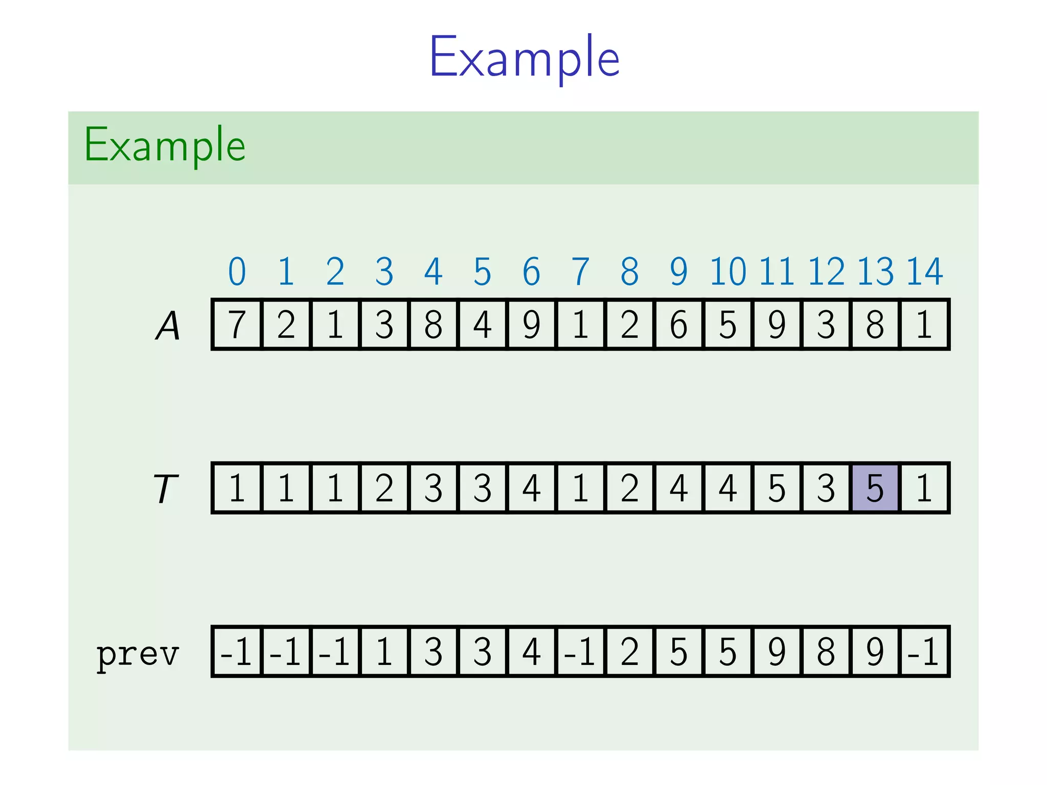
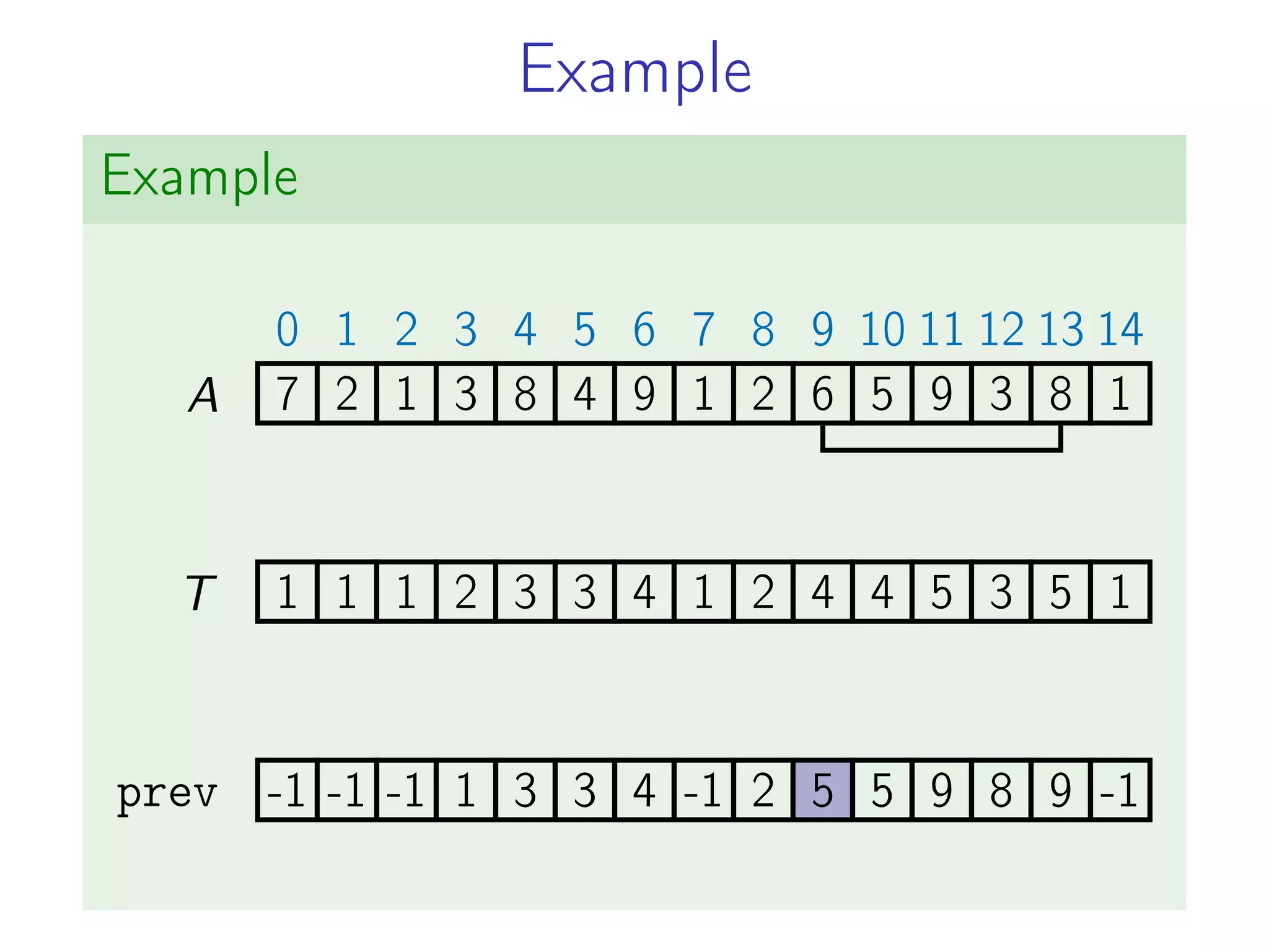
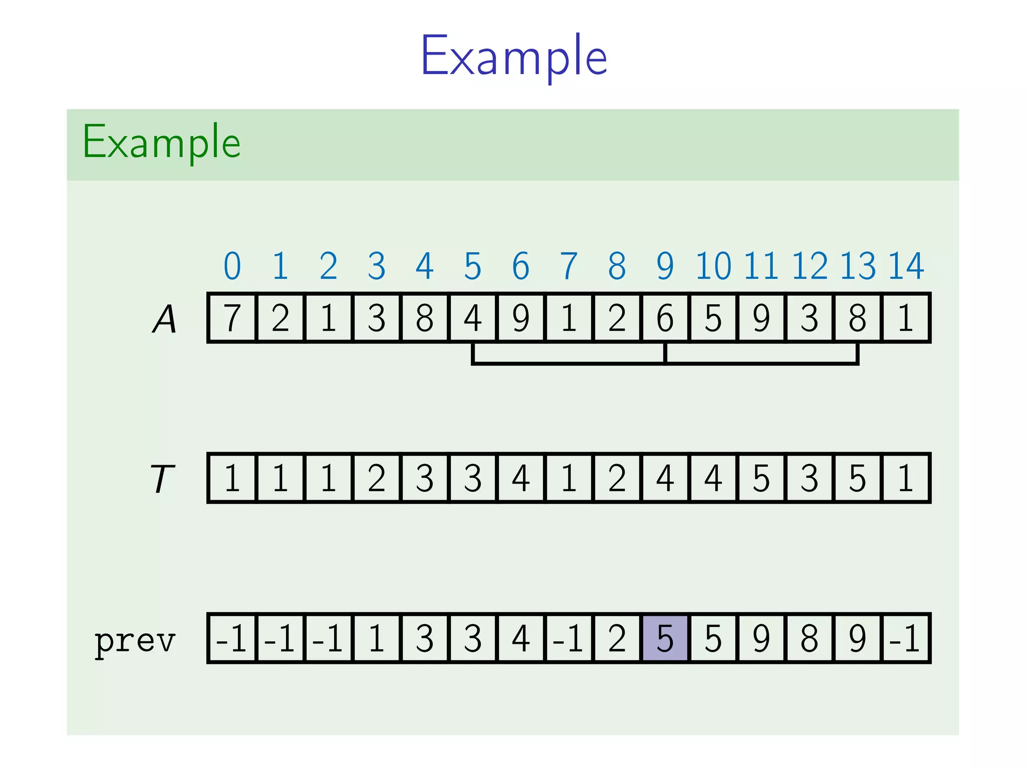
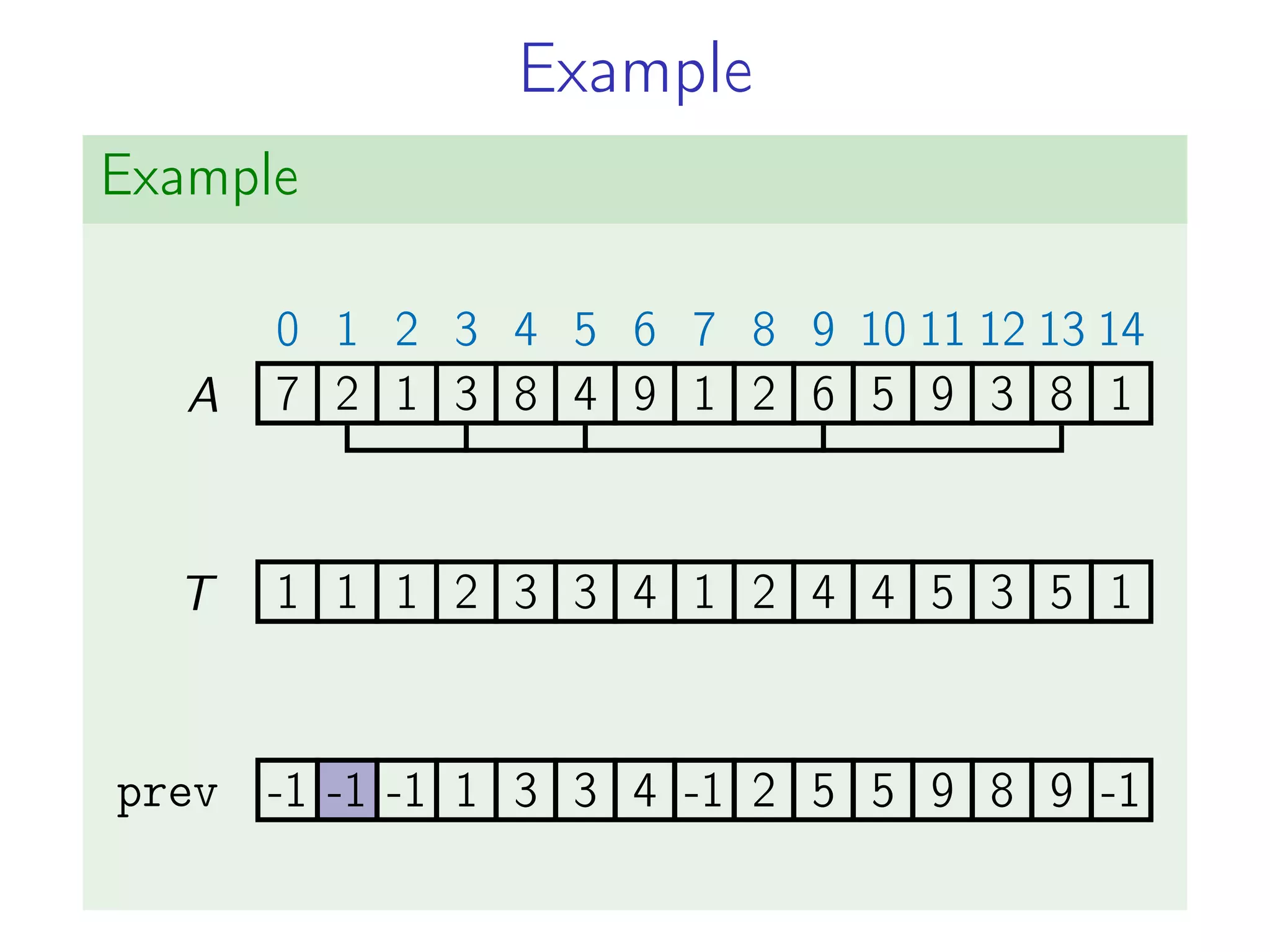
![Unwinding Solution
1 l a s t = 0
2 for i in range (1 , len (A ) ) :
3 i f T[ i ] > T[ l a s t ] :
4 l a s t = i
5
6 l i s= [ ]
7 c u r r e n t = l a s t
8 while c u r r e n t >= 0:
9 l i s . append ( c u r r e n t )
10 c u r r e n t = prev [ c u r r e n t ]
11 l i s . r e v e r s e ()
12 return [A[ i ] for i in l i s ]](https://image.slidesharecdn.com/dynamicprograming-220116082321/75/Dynamic-programing-77-2048.jpg)


![Brute Force: Code
1 def l i s (A, seq ) :
2 r e s u l t = len ( seq )
3
4 i f len ( seq ) == 0:
5 last_index = −1
6 last_element = float ( "−i n f " )
7 else :
8 last_index = seq [ −1]
9 last_element = A[ last_index ]
10
11 for i in range ( last_index + 1 , len (A ) ) :
12 i f A[ i ] > last_element :
13 r e s u l t = max( r e s u l t , l i s (A, seq + [ i ] ) )
14
15 return r e s u l t
16
17 print ( l i s (A=[7 , 2 , 1 , 3 , 8 , 4 , 9] , seq =[]))](https://image.slidesharecdn.com/dynamicprograming-220116082321/75/Dynamic-programing-98-2048.jpg)
![Optimized Code
1 def l i s (A, seq_len , last_index ) :
2 i f last_index == −1:
3 last_element = float ( "−i n f " )
4 else :
5 last_element = A[ last_index ]
6
7 r e s u l t = seq_len
8
9 for i in range ( last_index + 1 , len (A ) ) :
10 i f A[ i ] > last_element :
11 r e s u l t = max( r e s u l t ,
12 l i s (A, seq_len + 1 , i ))
13
14 return r e s u l t
15
16 print ( l i s ( [ 3 , 2 , 7 , 8 , 9 , 5 , 8] , 0 , −1))](https://image.slidesharecdn.com/dynamicprograming-220116082321/75/Dynamic-programing-103-2048.jpg)
![Resulting Code
1 def l i s (A, last_index ) :
2 i f last_index == −1:
3 last_element = float ( "−i n f " )
4 else :
5 last_element = A[ last_index ]
6
7 r e s u l t = 0
8
9 for i in range ( last_index + 1 , len (A ) ) :
10 i f A[ i ] > last_element :
11 r e s u l t = max( r e s u l t , 1 + l i s (A, i ))
12
13 return r e s u l t
14
15 print ( l i s ( [ 8 , 2 , 3 , 4 , 5 , 6 , 7] , −1))](https://image.slidesharecdn.com/dynamicprograming-220116082321/75/Dynamic-programing-108-2048.jpg)
![Resulting Code
1 def l i s (A, last_index ) :
2 i f last_index == −1:
3 last_element = float ( "−i n f " )
4 else :
5 last_element = A[ last_index ]
6
7 r e s u l t = 0
8
9 for i in range ( last_index + 1 , len (A ) ) :
10 i f A[ i ] > last_element :
11 r e s u l t = max( r e s u l t , 1 + l i s (A, i ))
12
13 return r e s u l t
14
15 print ( l i s ( [ 8 , 2 , 3 , 4 , 5 , 6 , 7] , −1))
It remains to add memoization!](https://image.slidesharecdn.com/dynamicprograming-220116082321/75/Dynamic-programing-109-2048.jpg)
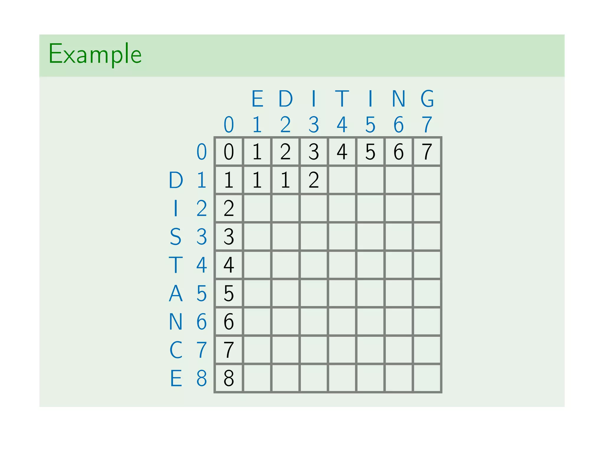
![Statement
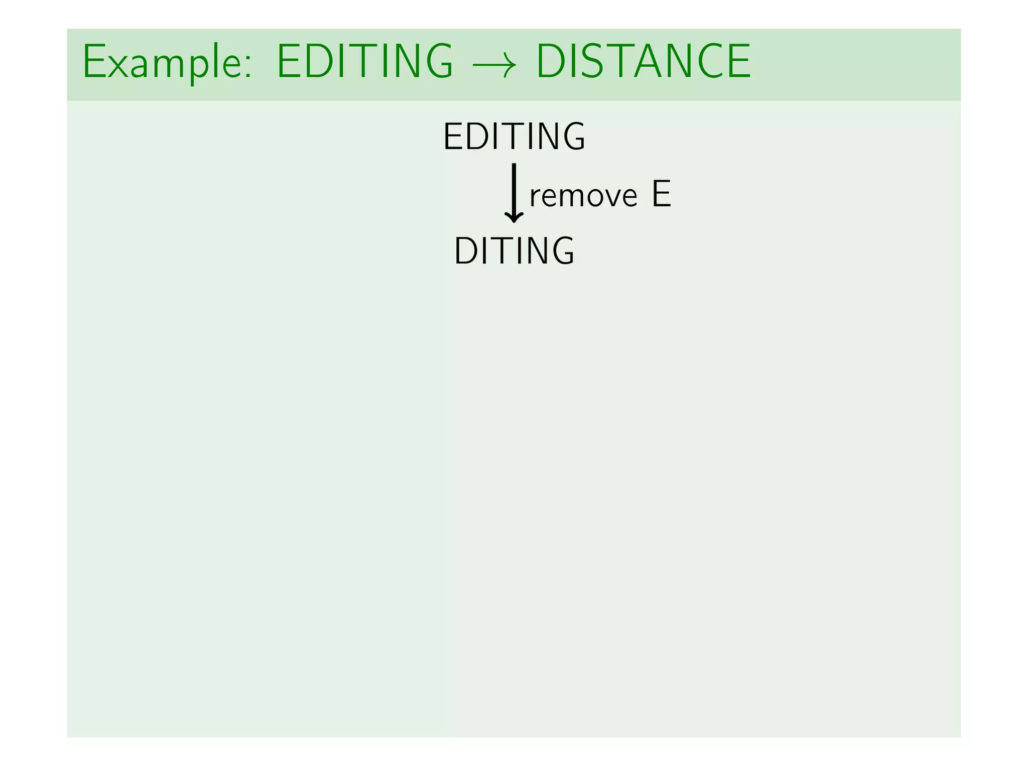
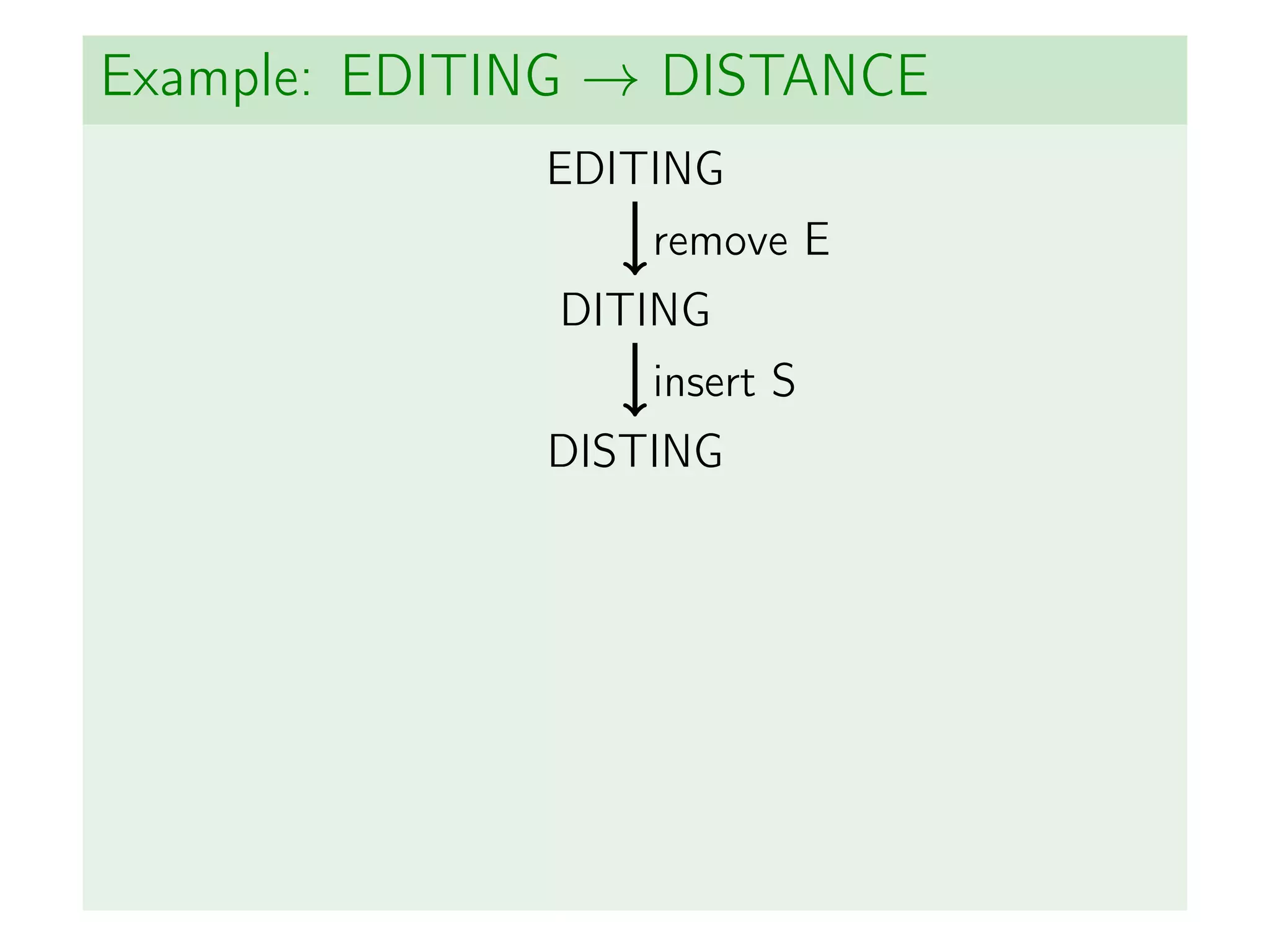
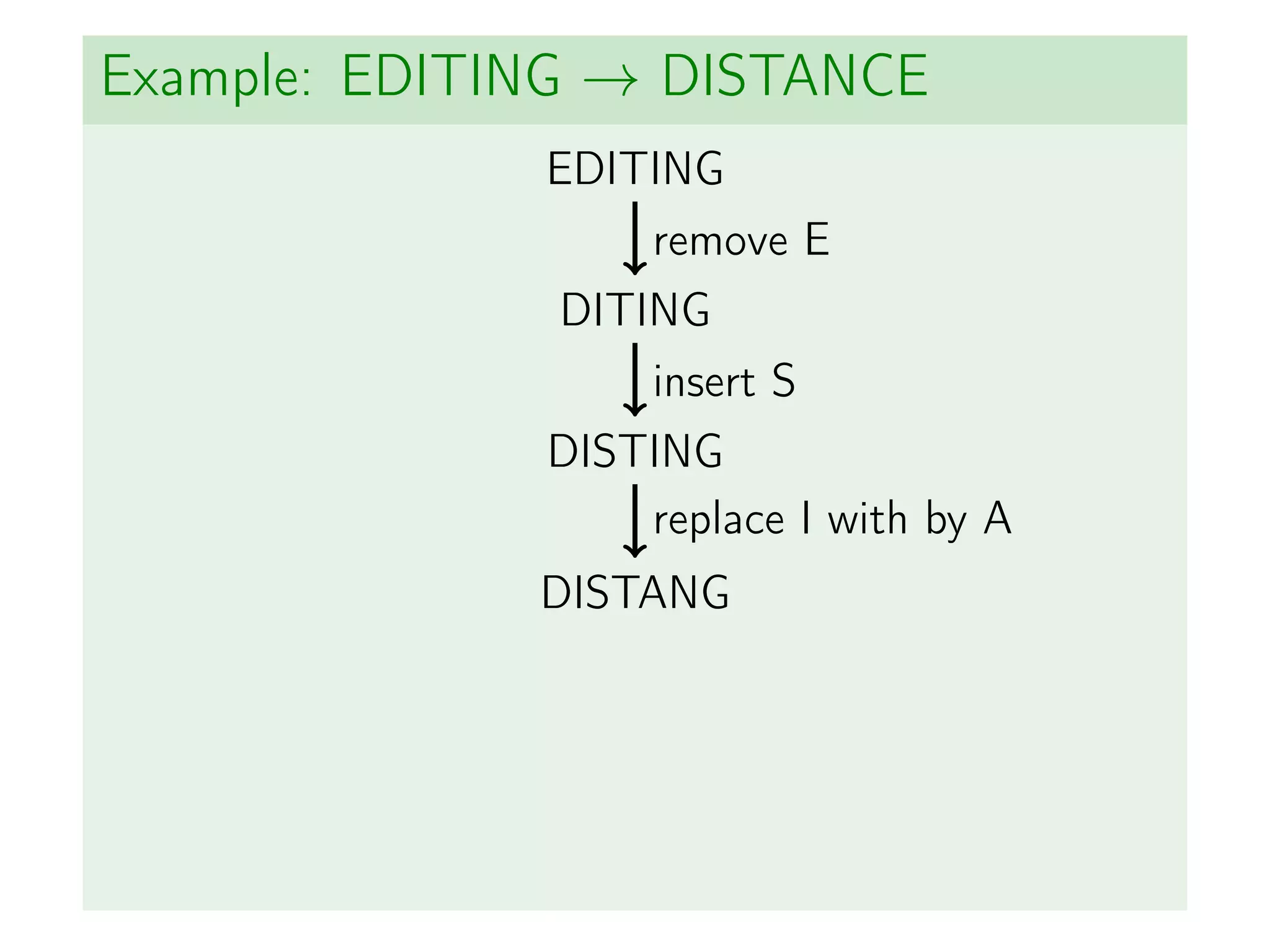
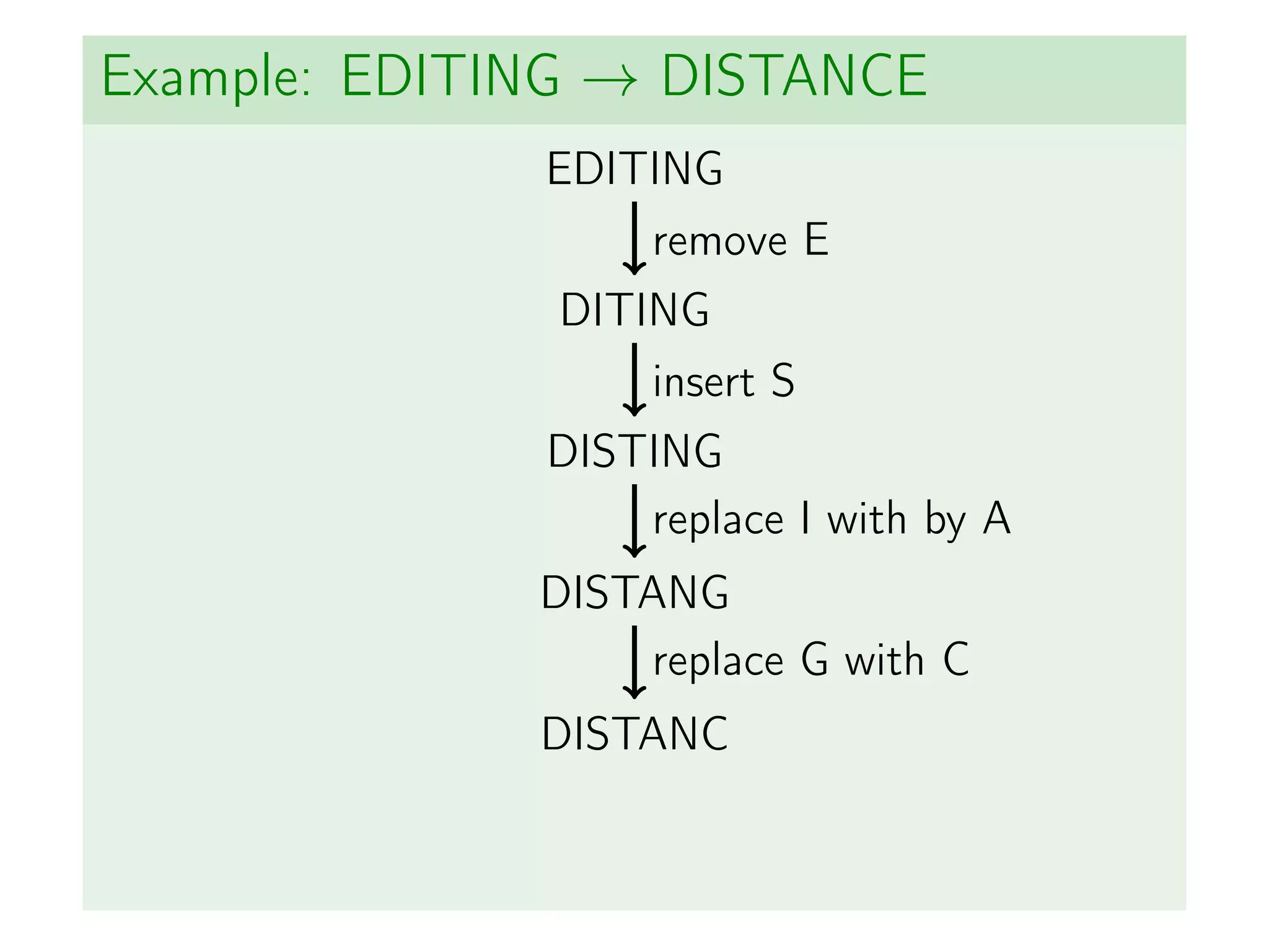
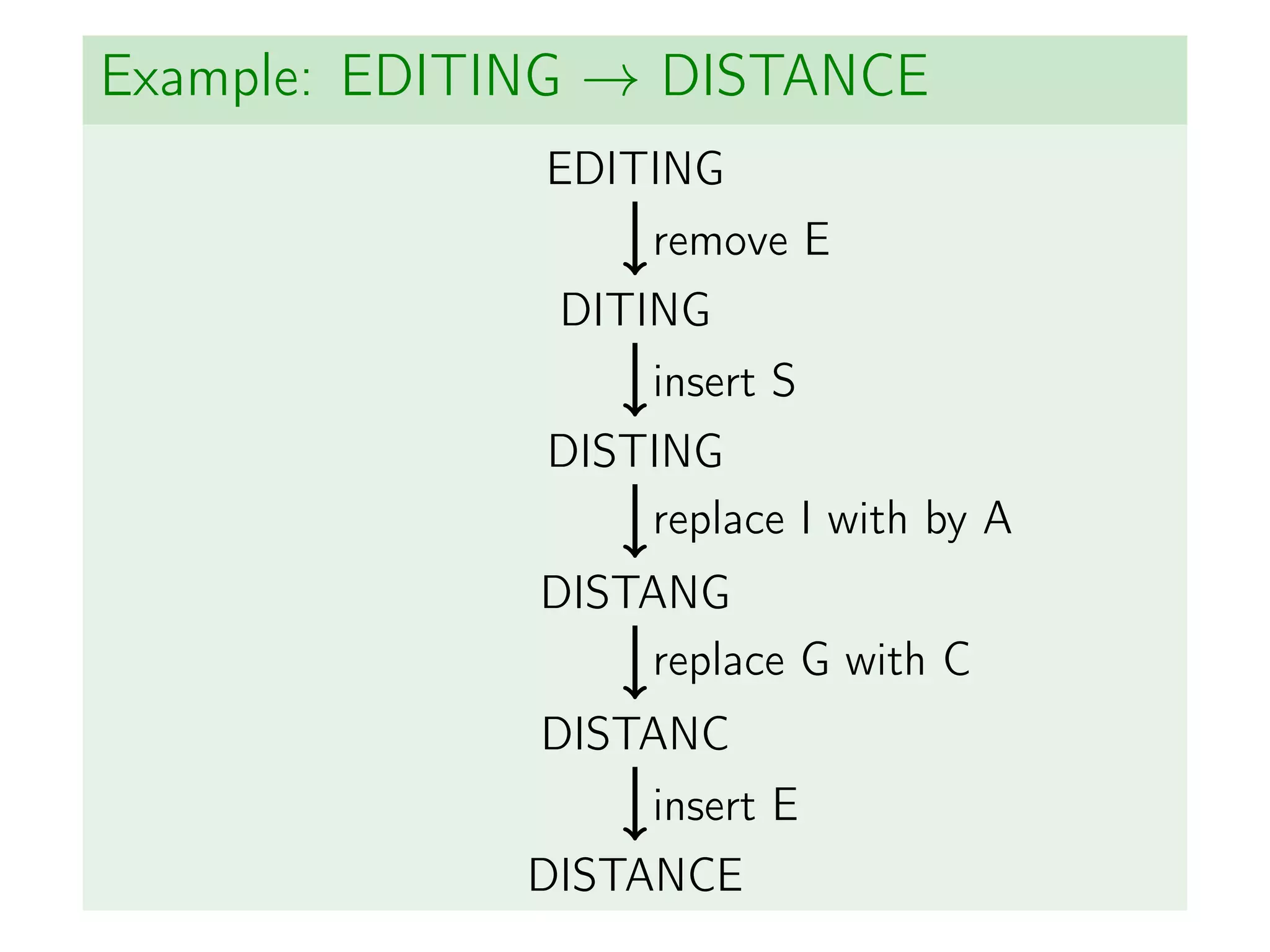
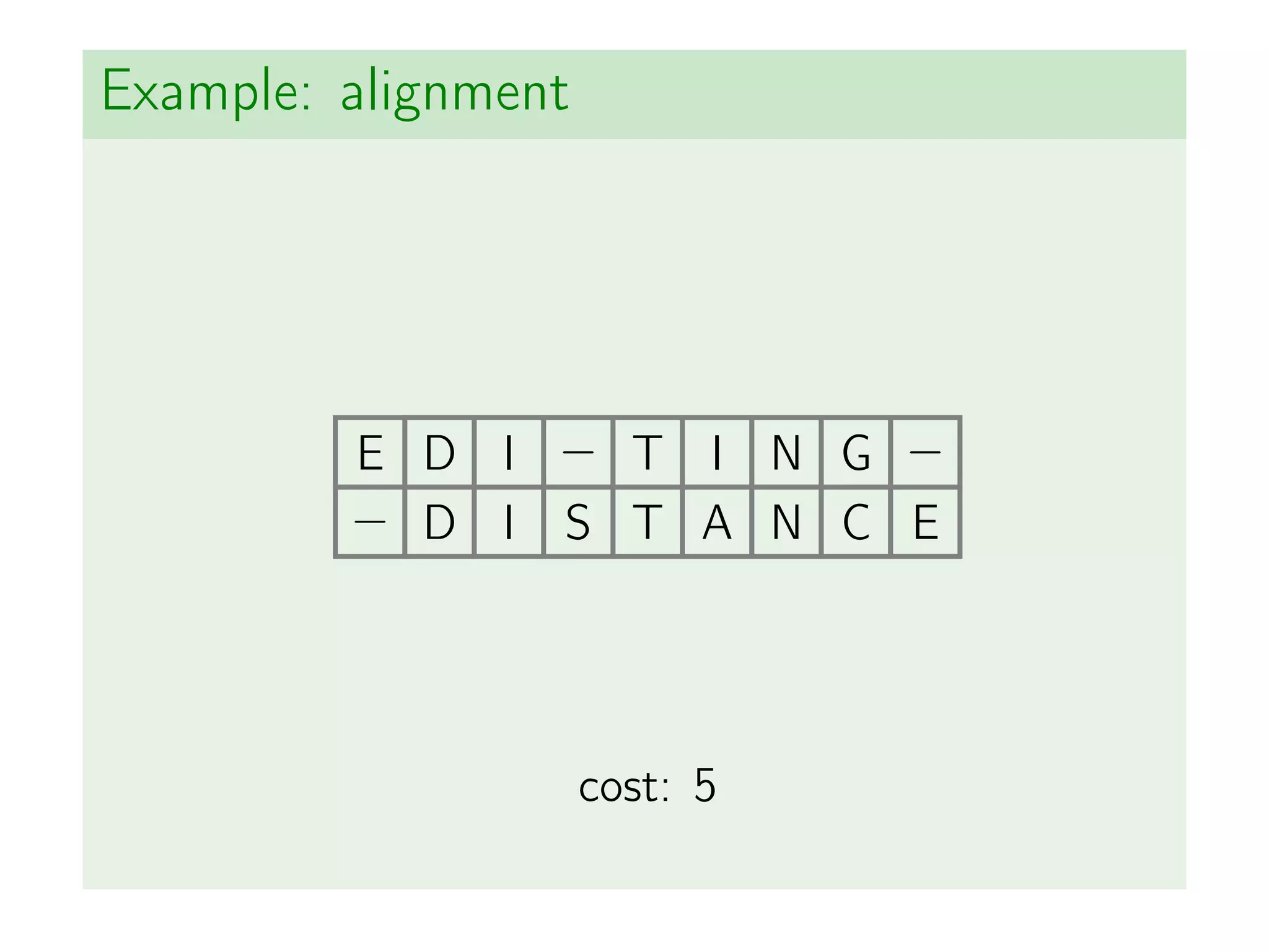
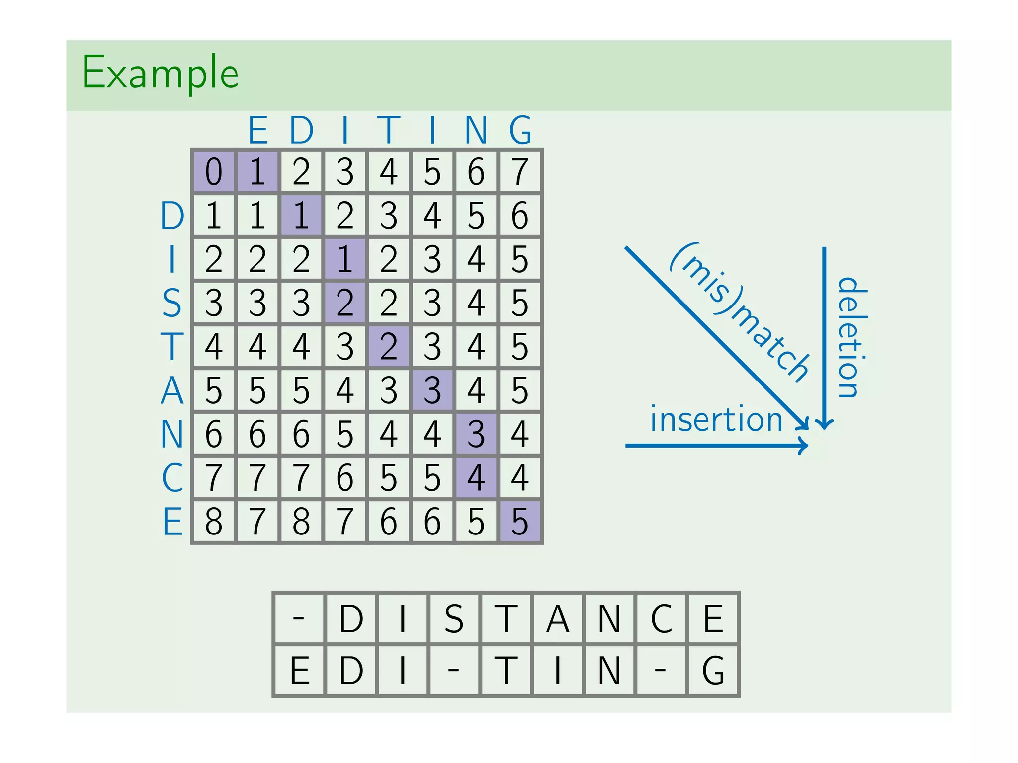
Edit distance
Input: Two strings A[0 . . . n − 1] and
B[0 . . . m − 1].
Output: The minimal number of insertions,
deletions, and substitutions needed to
transform A to B. This number is known
as edit distance or Levenshtein distance.](https://image.slidesharecdn.com/dynamicprograming-220116082321/75/Dynamic-programing-115-2048.jpg)
![Analyzing an Optimal Alignment
A[0 . . . n − 1]
B[0 . . . m − 1]](https://image.slidesharecdn.com/dynamicprograming-220116082321/75/Dynamic-programing-124-2048.jpg)
![Analyzing an Optimal Alignment
A[0 . . . n − 1]
B[0 . . . m − 1]
A[0 . . . n − 1] −
B[0 . . . m − 2] B[m − 1]
insertion](https://image.slidesharecdn.com/dynamicprograming-220116082321/75/Dynamic-programing-125-2048.jpg)
![Analyzing an Optimal Alignment
A[0 . . . n − 1]
B[0 . . . m − 1]
A[0 . . . n − 1] −
B[0 . . . m − 2] B[m − 1]
insertion
A[0 . . . n − 2] A[n − 1]
B[0 . . . m − 1] −
deletion](https://image.slidesharecdn.com/dynamicprograming-220116082321/75/Dynamic-programing-126-2048.jpg)
![Analyzing an Optimal Alignment
A[0 . . . n − 1]
B[0 . . . m − 1]
A[0 . . . n − 1] −
B[0 . . . m − 2] B[m − 1]
insertion
A[0 . . . n − 2] A[n − 1]
B[0 . . . m − 1] −
deletion
A[0 . . . n − 2] A[n − 1]
B[0 . . . m − 2] B[m − 1]
match/mismatch](https://image.slidesharecdn.com/dynamicprograming-220116082321/75/Dynamic-programing-127-2048.jpg)
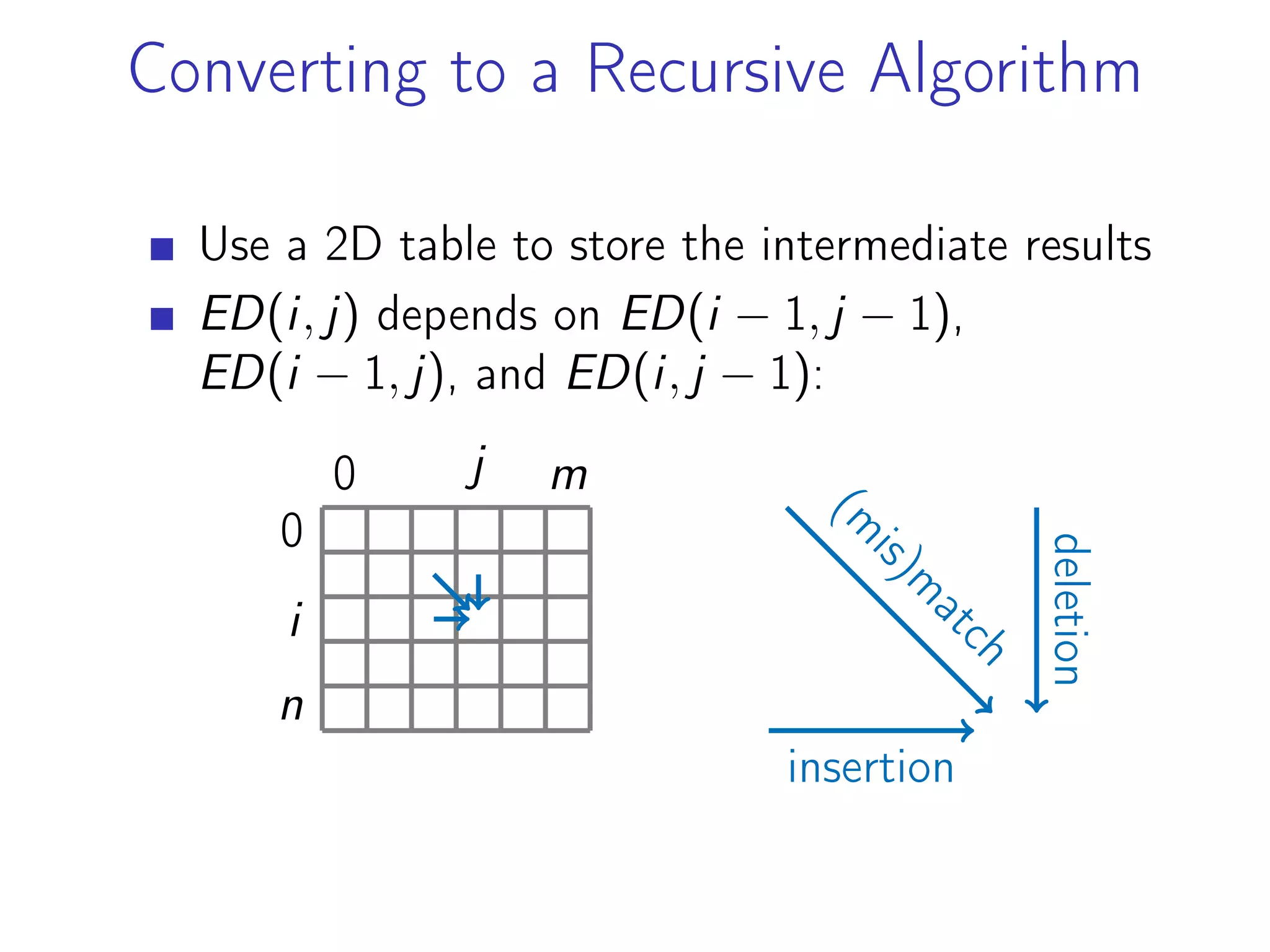
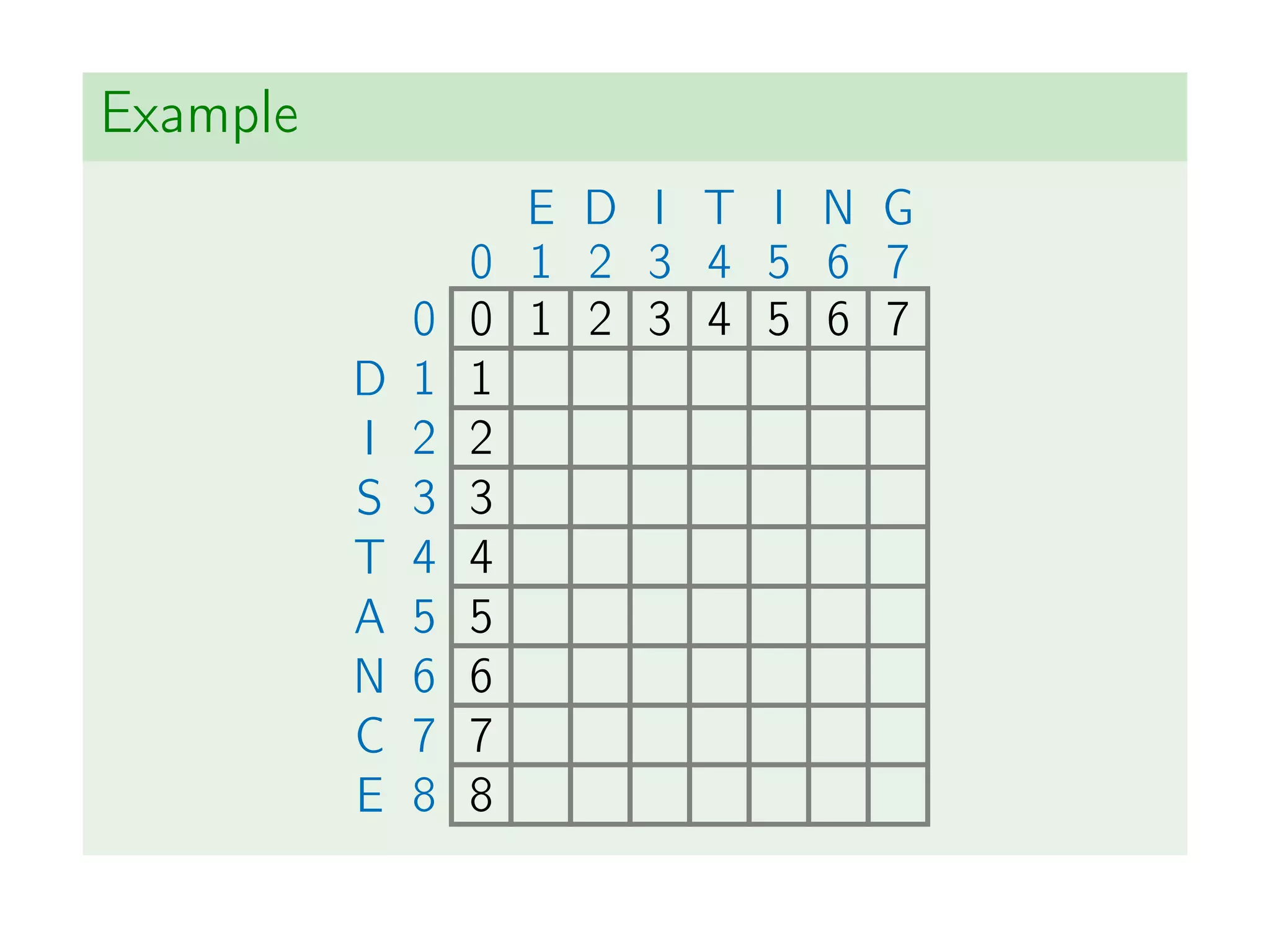
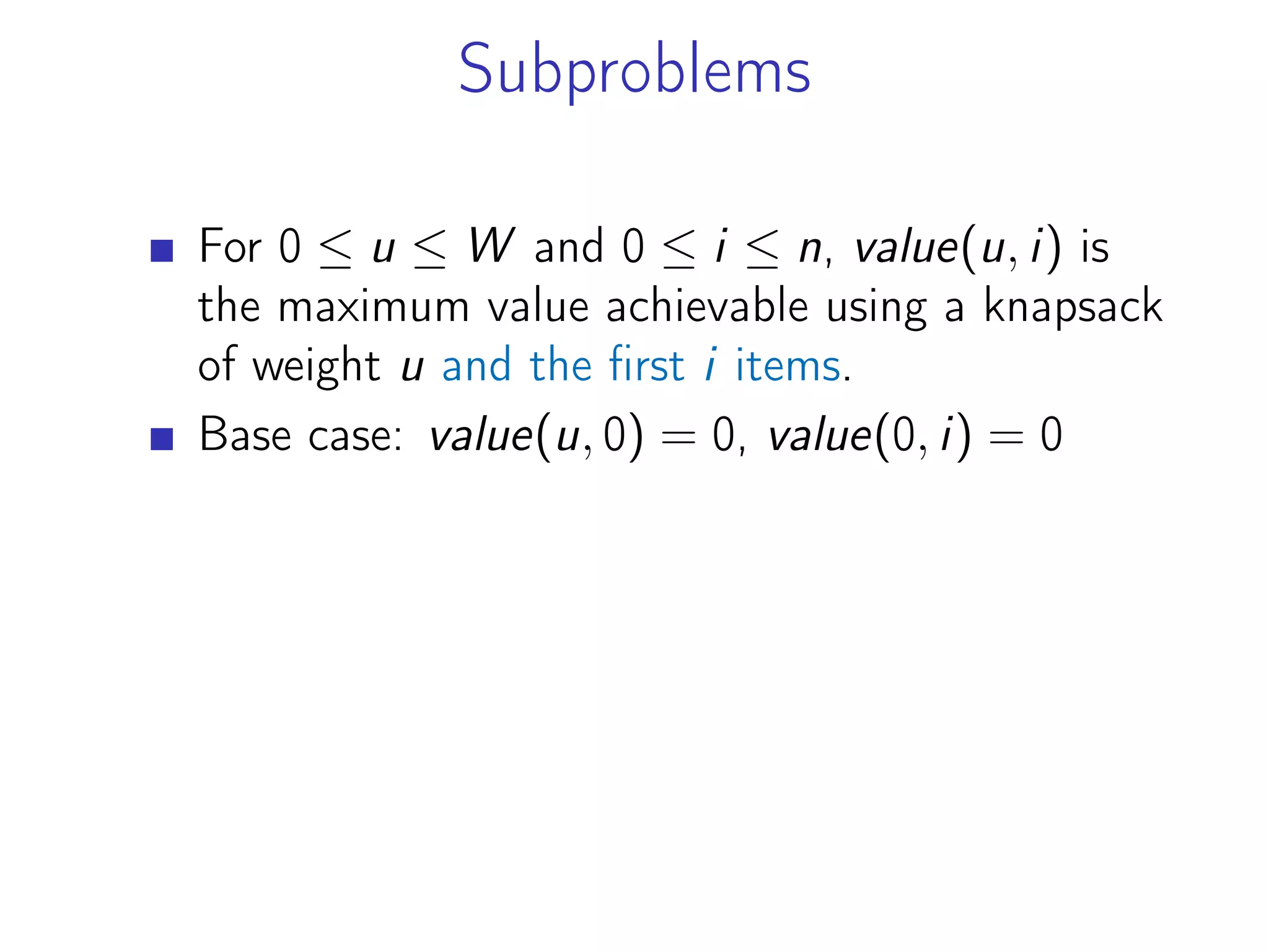
![Subproblems
Let ED(i, j) be the edit distance of
A[0 . . . i − 1] and B[0 . . . j − 1].](https://image.slidesharecdn.com/dynamicprograming-220116082321/75/Dynamic-programing-128-2048.jpg)
![Subproblems
Let ED(i, j) be the edit distance of
A[0 . . . i − 1] and B[0 . . . j − 1].
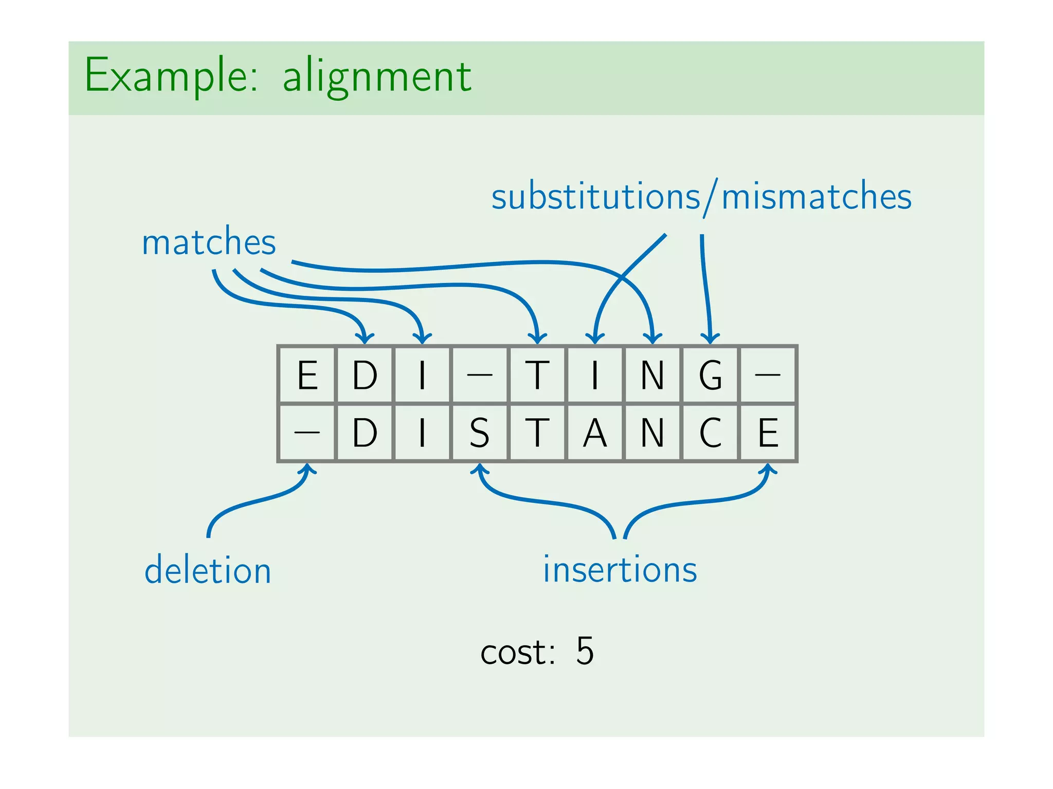
We know for sure that the last column of an
optimal alignment is either an insertion, a
deletion, or a match/mismatch.](https://image.slidesharecdn.com/dynamicprograming-220116082321/75/Dynamic-programing-129-2048.jpg)
![Subproblems
Let ED(i, j) be the edit distance of
A[0 . . . i − 1] and B[0 . . . j − 1].
We know for sure that the last column of an
optimal alignment is either an insertion, a
deletion, or a match/mismatch.
What is left is an optimal alignment of the
corresponding two prefixes (by cut-and-paste).](https://image.slidesharecdn.com/dynamicprograming-220116082321/75/Dynamic-programing-130-2048.jpg)
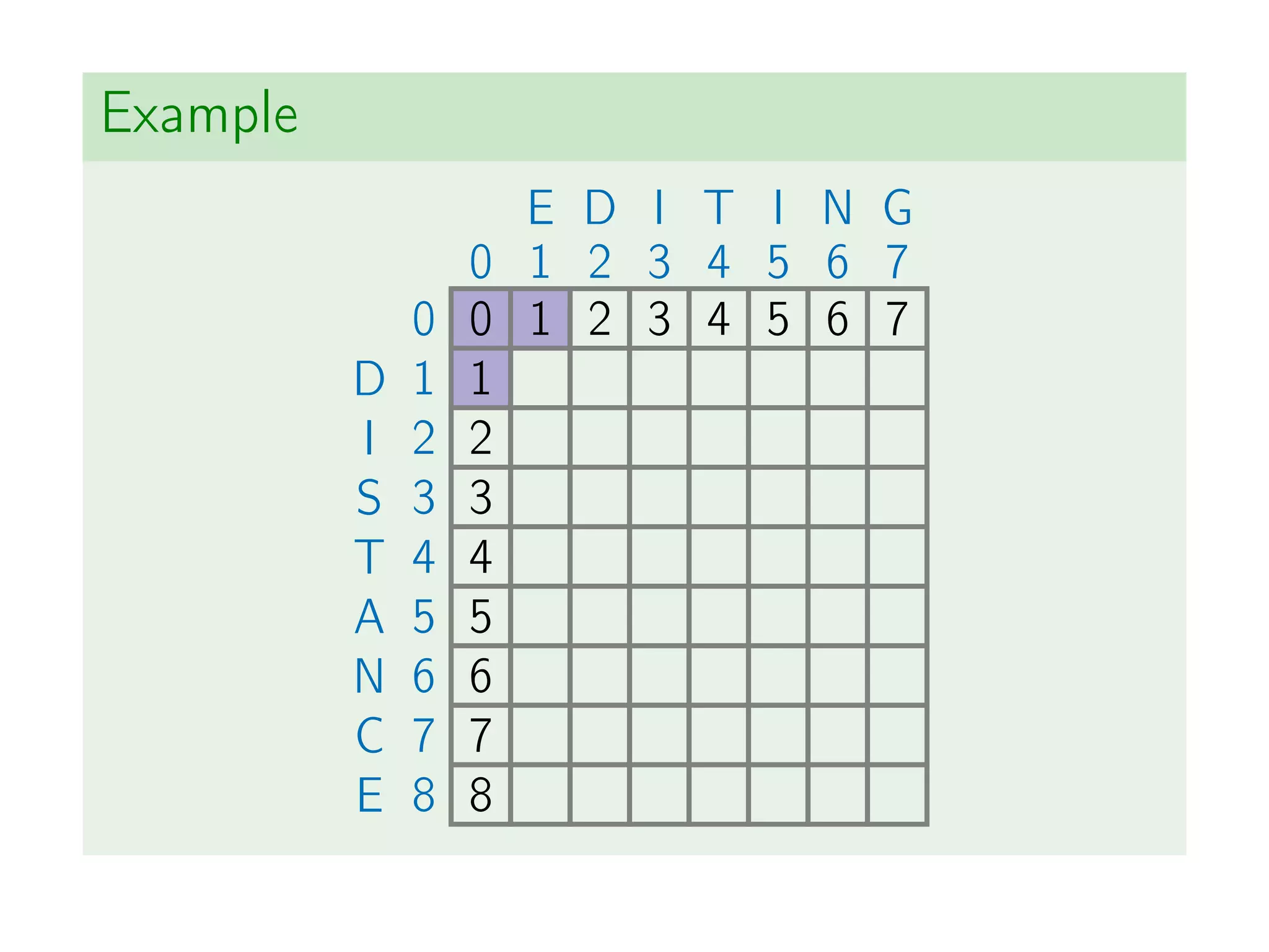
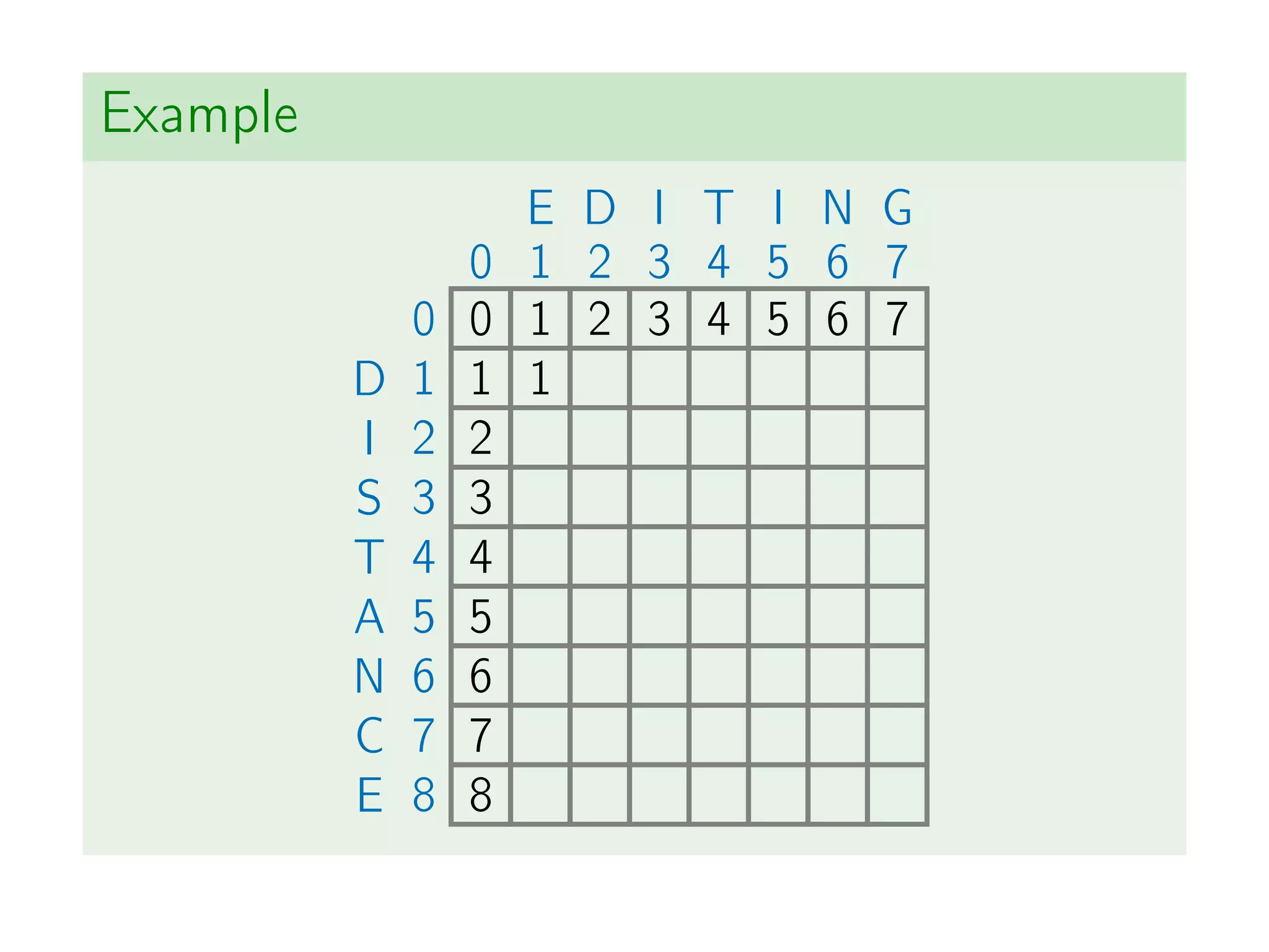
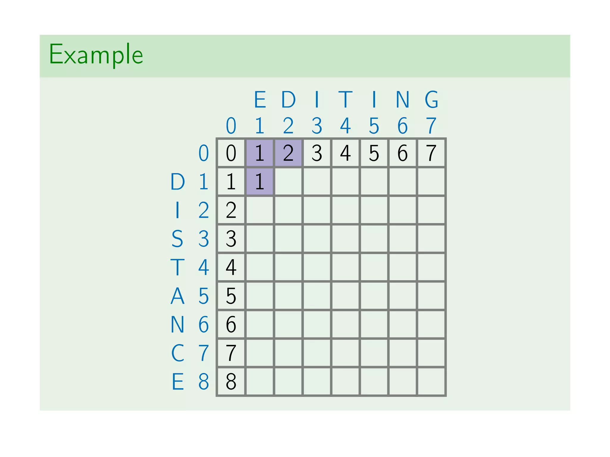
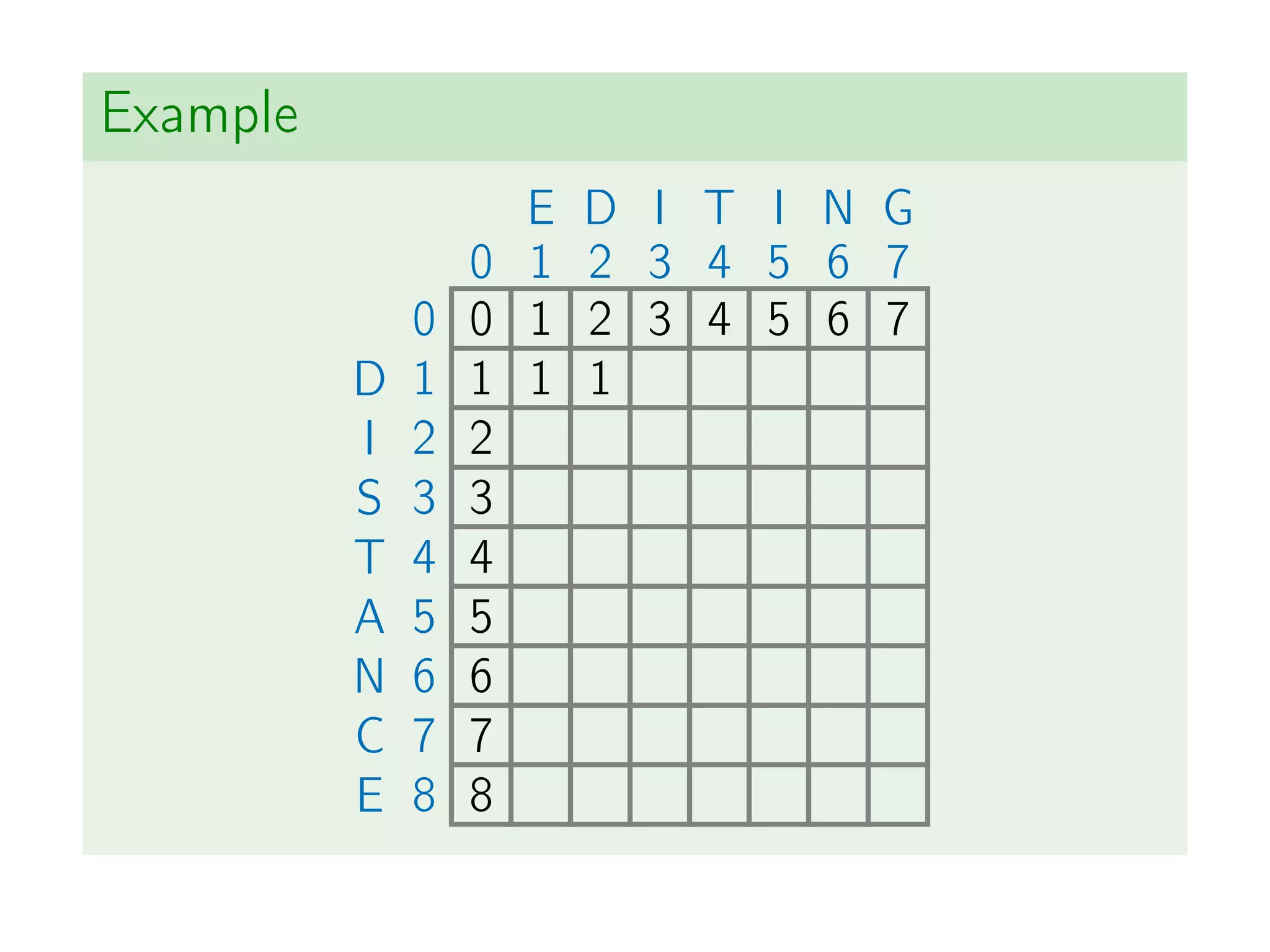
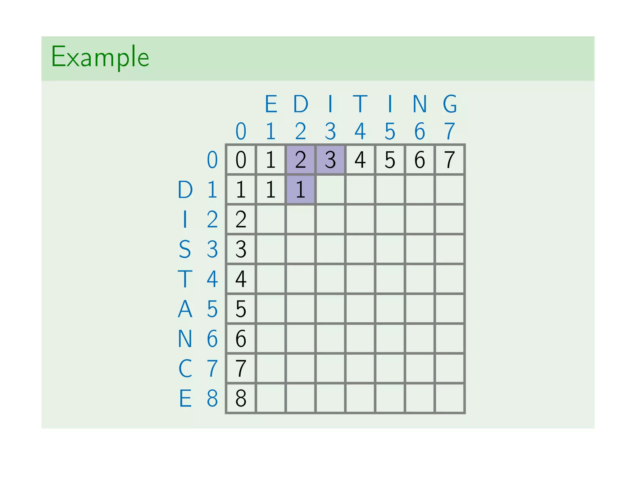
![Recurrence Relation
ED(i, j) = min
⎧
⎪
⎨
⎪
⎩
ED(i, j − 1) + 1
ED(i − 1, j) + 1
ED(i − 1, j − 1) + diff(A[i], B[j])](https://image.slidesharecdn.com/dynamicprograming-220116082321/75/Dynamic-programing-131-2048.jpg)
![Recurrence Relation
ED(i, j) = min
⎧
⎪
⎨
⎪
⎩
ED(i, j − 1) + 1
ED(i − 1, j) + 1
ED(i − 1, j − 1) + diff(A[i], B[j])
Base case: ED(i, 0) = i, ED(0, j) = j](https://image.slidesharecdn.com/dynamicprograming-220116082321/75/Dynamic-programing-132-2048.jpg)
![Recursive Algorithm
1 T = dict ()
2
3 def edit_distance (a , b , i , j ) :
4 i f not ( i , j ) in T:
5 i f i == 0: T[ i , j ] = j
6 e l i f j == 0: T[ i , j ] = i
7 else :
8 d i f f = 0 i f a [ i − 1] == b [ j − 1] else 1
9 T[ i , j ] = min(
10 edit_distance (a , b , i − 1 , j ) + 1 ,
11 edit_distance (a , b , i , j − 1) + 1 ,
12 edit_distance (a , b , i − 1 , j − 1) + d i f f )
13
14 return T[ i , j ]
15
16
17 print ( edit_distance ( a=" e d i t i n g " , b=" d i s t a n c e " ,
18 i =7, j =8))](https://image.slidesharecdn.com/dynamicprograming-220116082321/75/Dynamic-programing-133-2048.jpg)
![Iterative Algorithm
1 def edit_distance (a , b ) :
2 T = [ [ f l o a t ( " i n f " ) ] * ( len (b) + 1)
3 for _ in range ( len ( a ) + 1 ) ]
4 for i in range ( len ( a ) + 1 ) :
5 T[ i ] [ 0 ] = i
6 for j in range ( len (b) + 1 ) :
7 T [ 0 ] [ j ] = j
8
9 for i in range (1 , len ( a ) + 1 ) :
10 for j in range (1 , len (b) + 1 ) :
11 d i f f = 0 i f a [ i − 1] == b [ j − 1] else 1
12 T[ i ] [ j ] = min(T[ i − 1 ] [ j ] + 1 ,
13 T[ i ] [ j − 1] + 1 ,
14 T[ i − 1 ] [ j − 1] + d i f f )
15
16 return T[ len ( a ) ] [ len (b ) ]
17
18
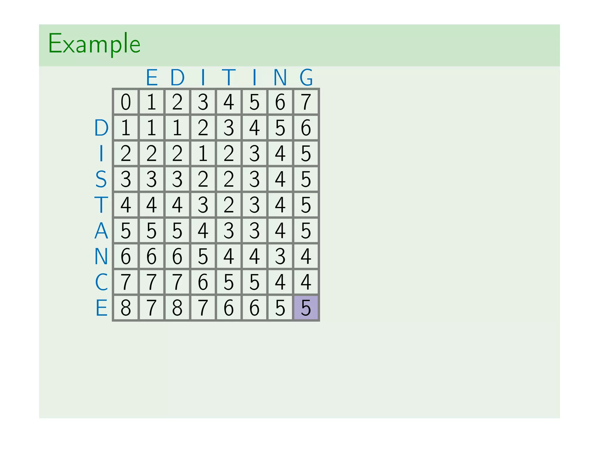
19 print ( edit_distance ( a=" d i s t a n c e " , b=" e d i t i n g " ))](https://image.slidesharecdn.com/dynamicprograming-220116082321/75/Dynamic-programing-137-2048.jpg)
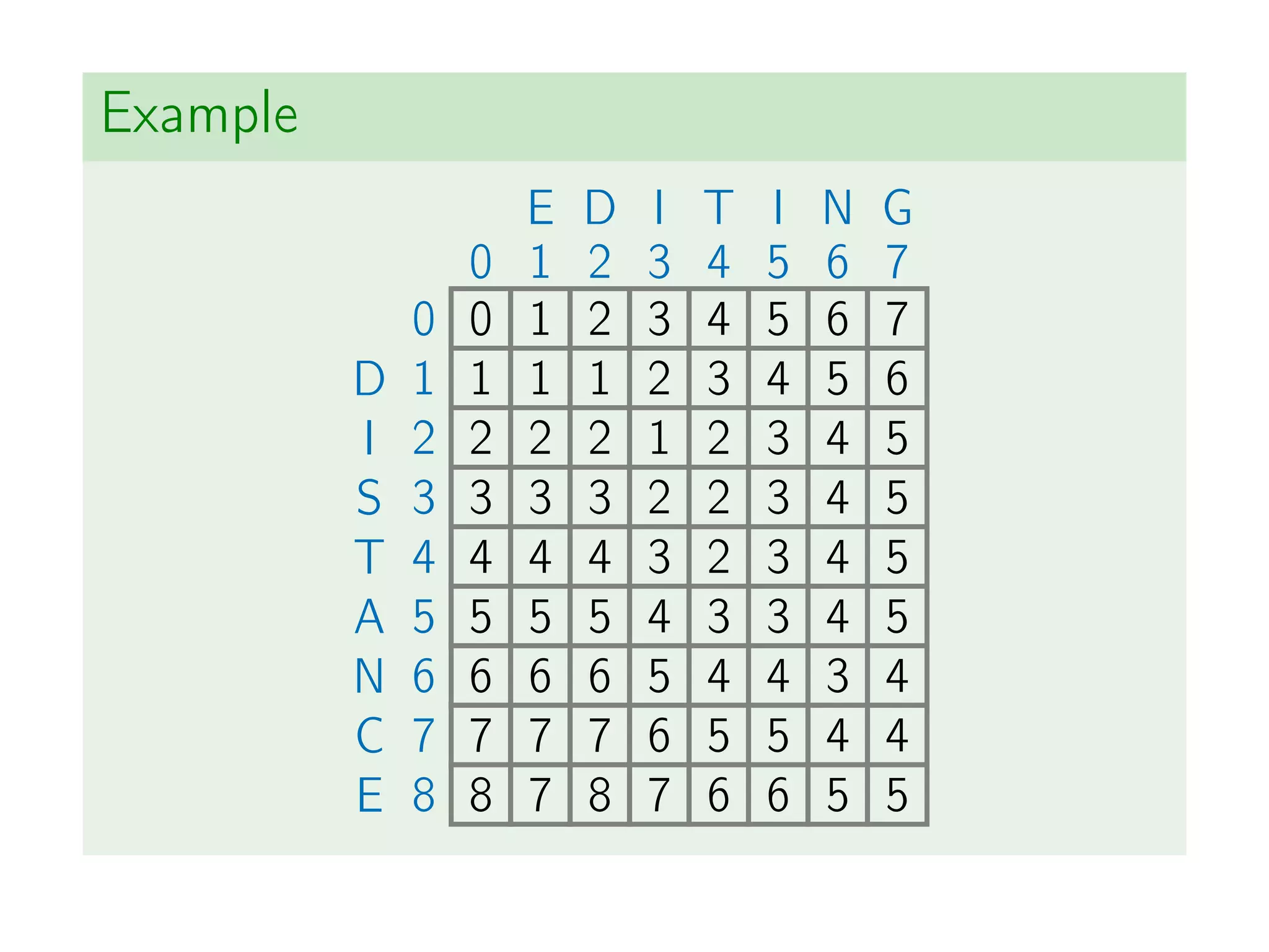

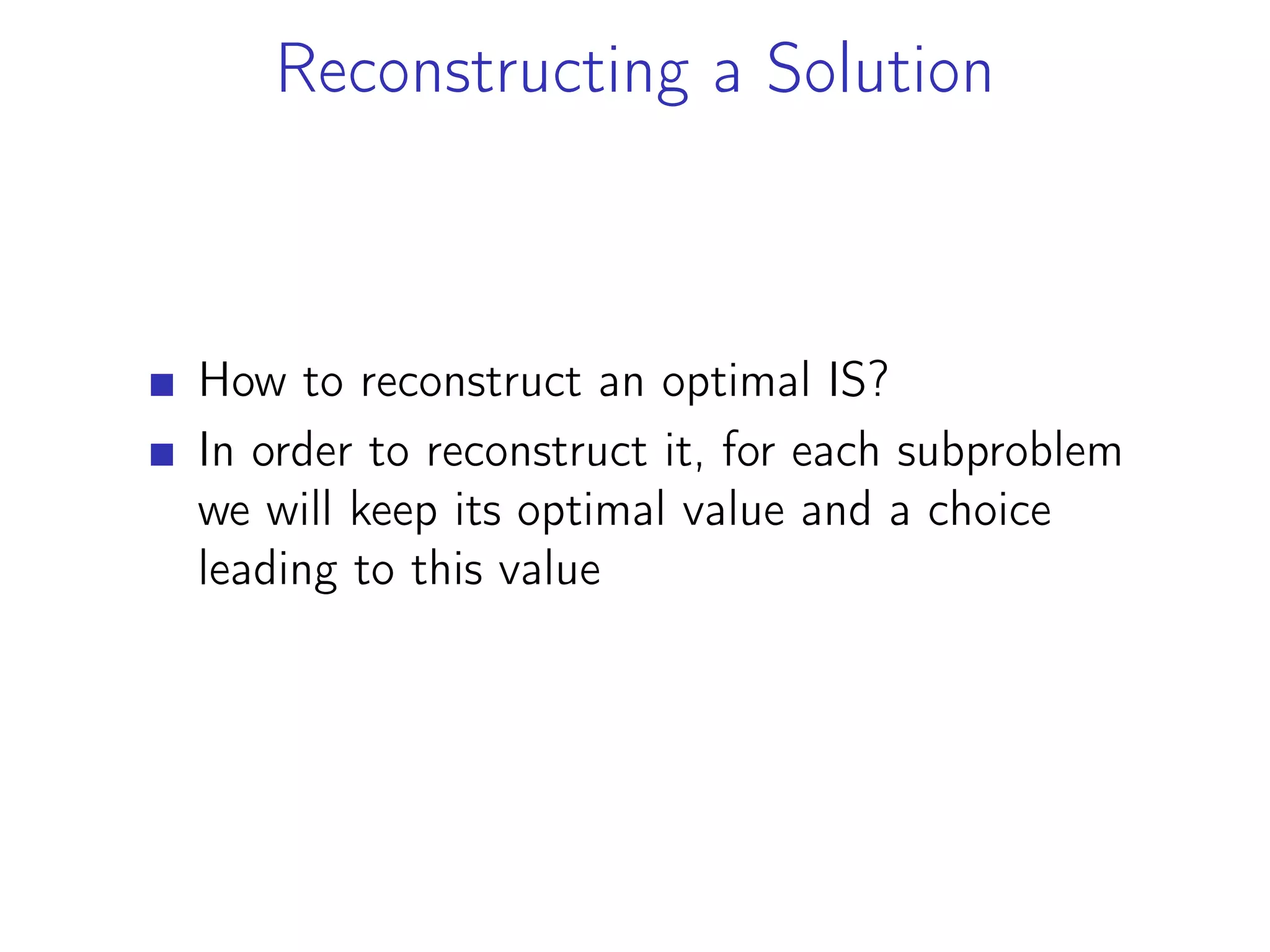
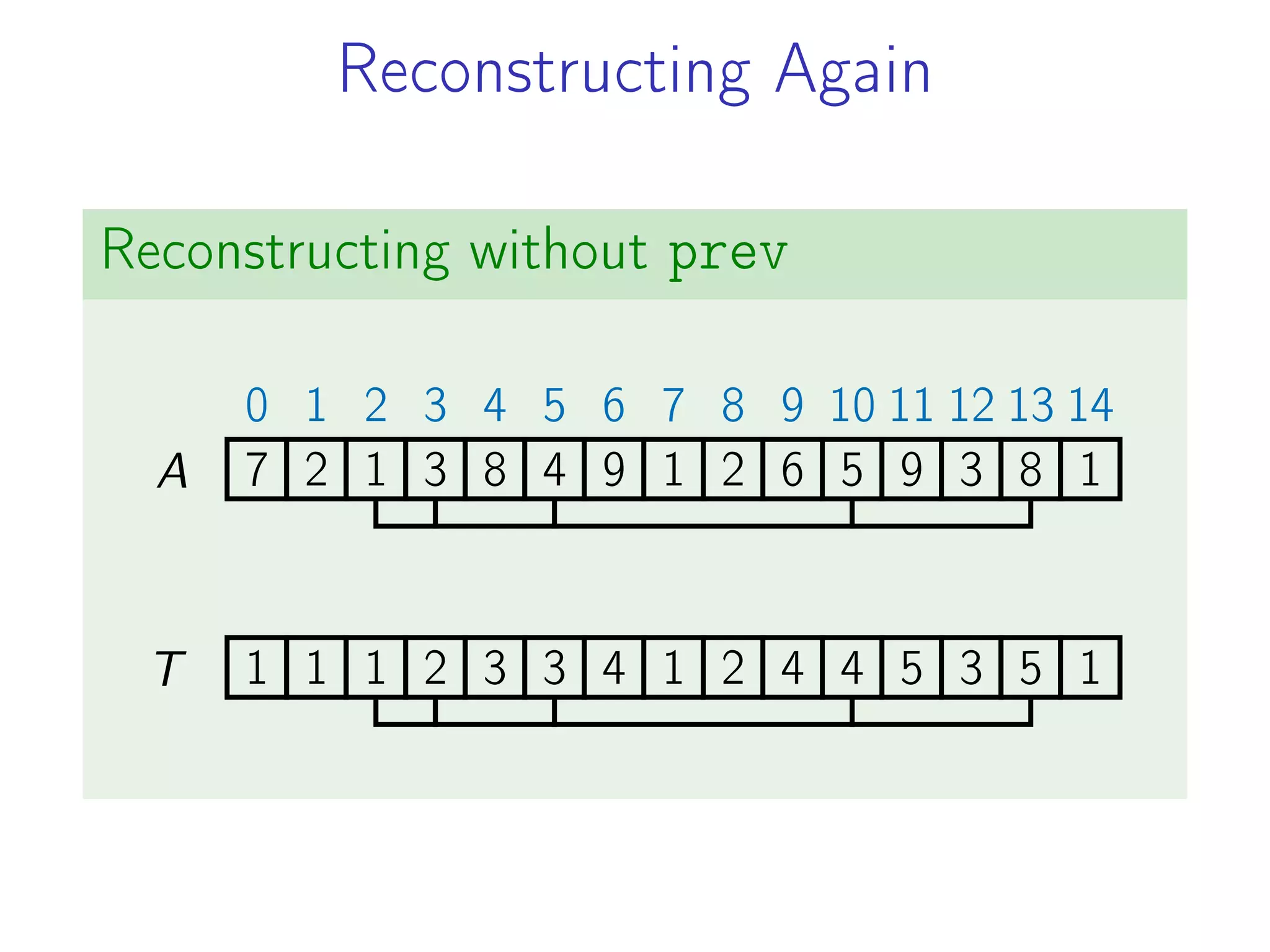
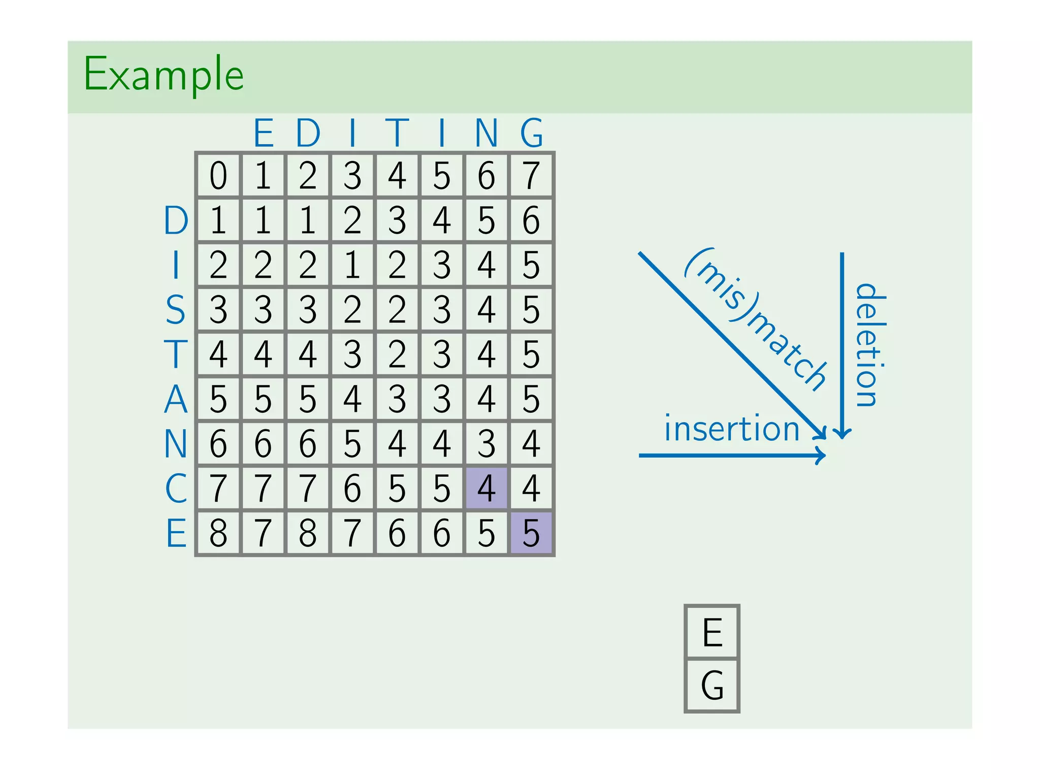
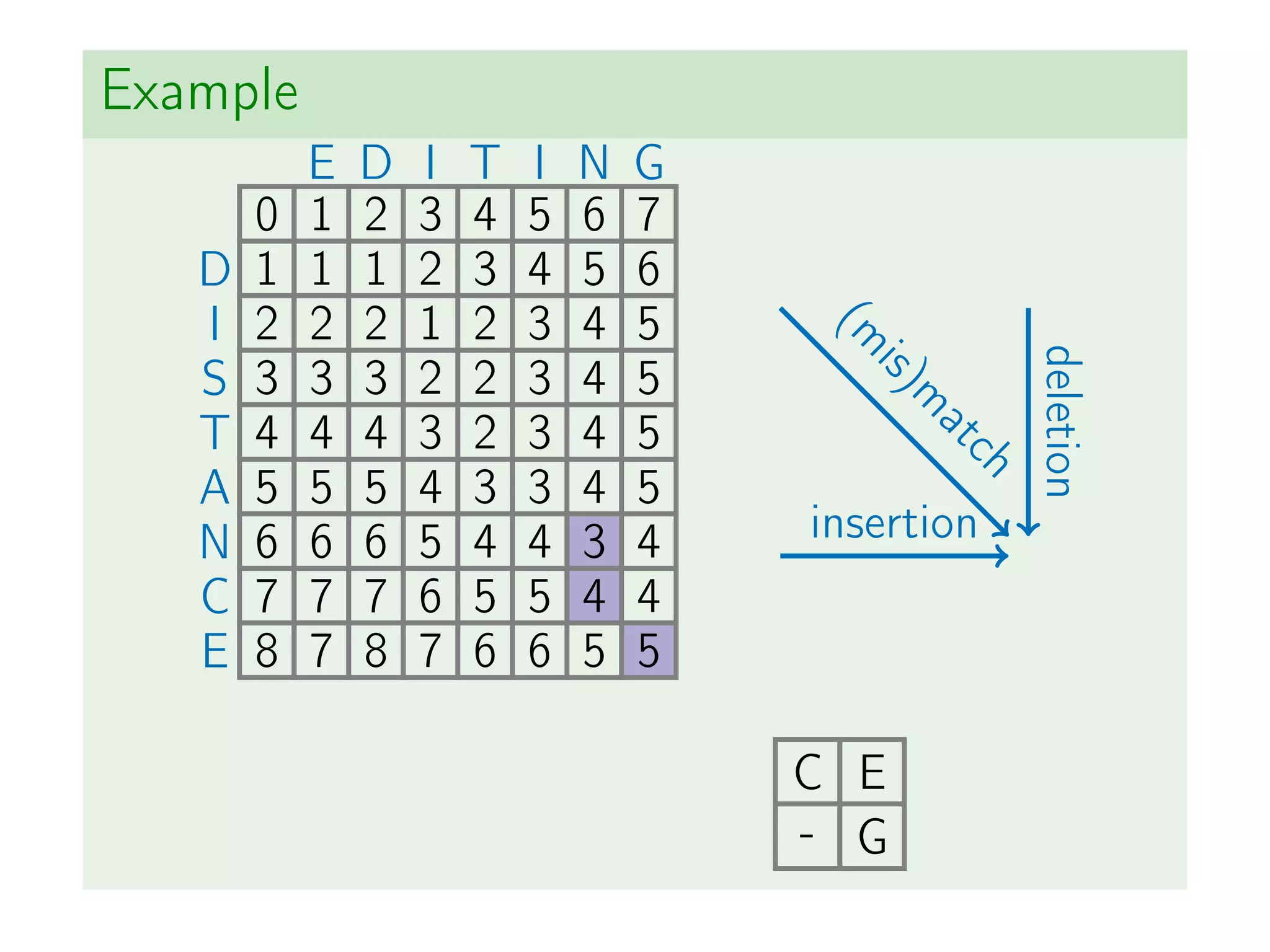
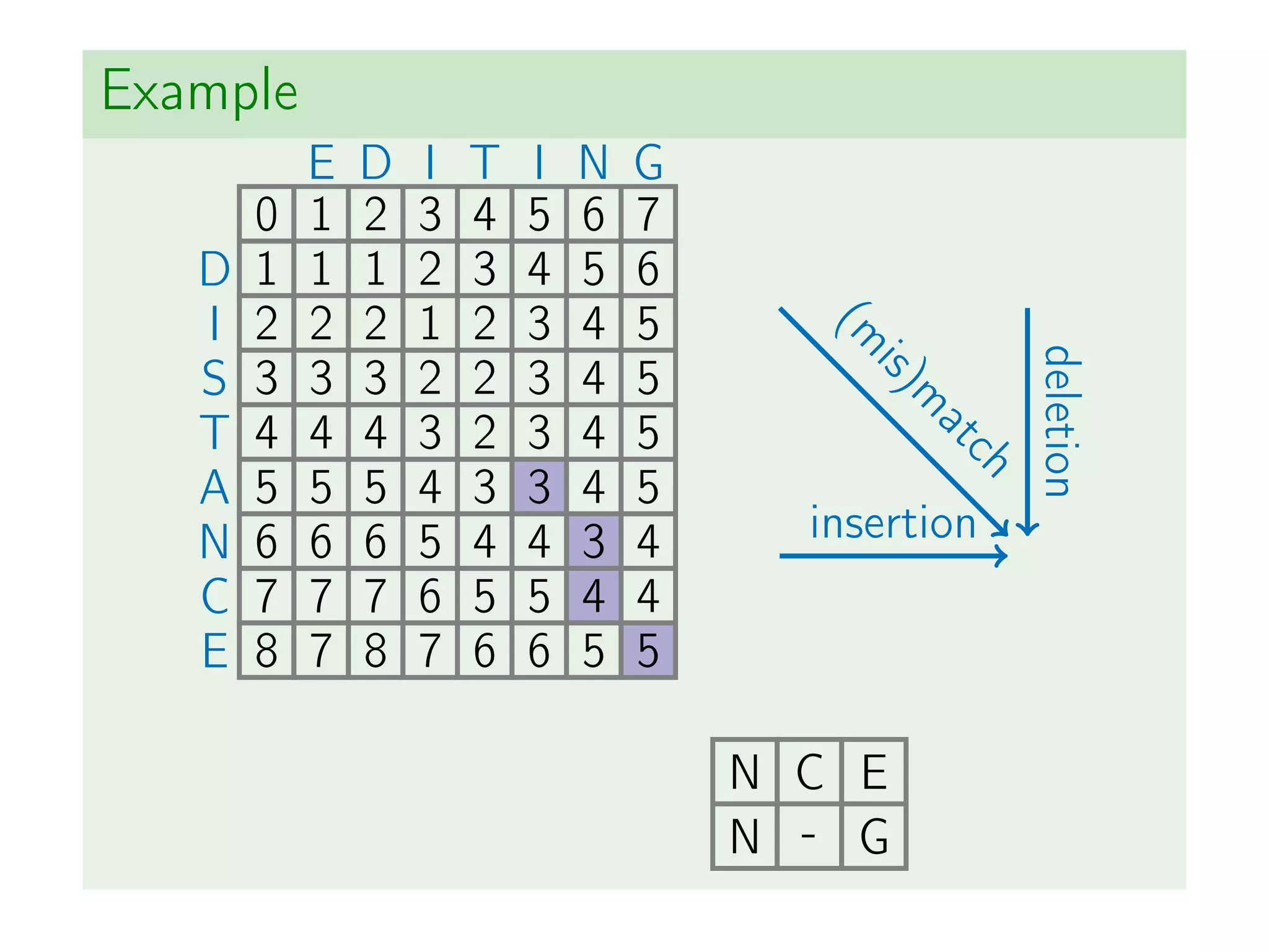
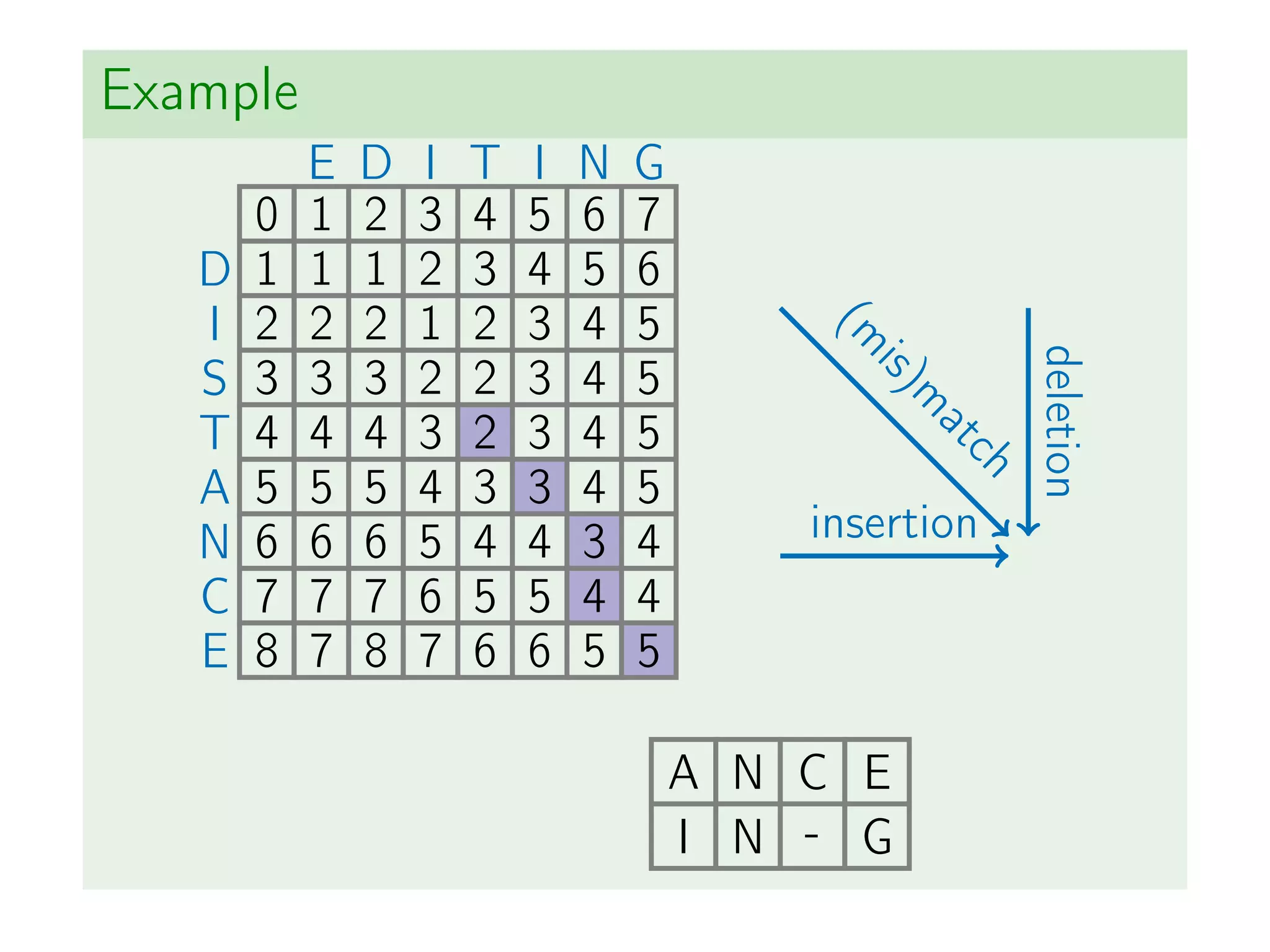
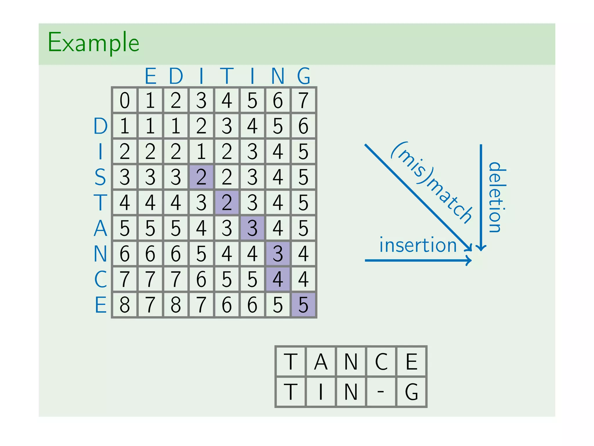
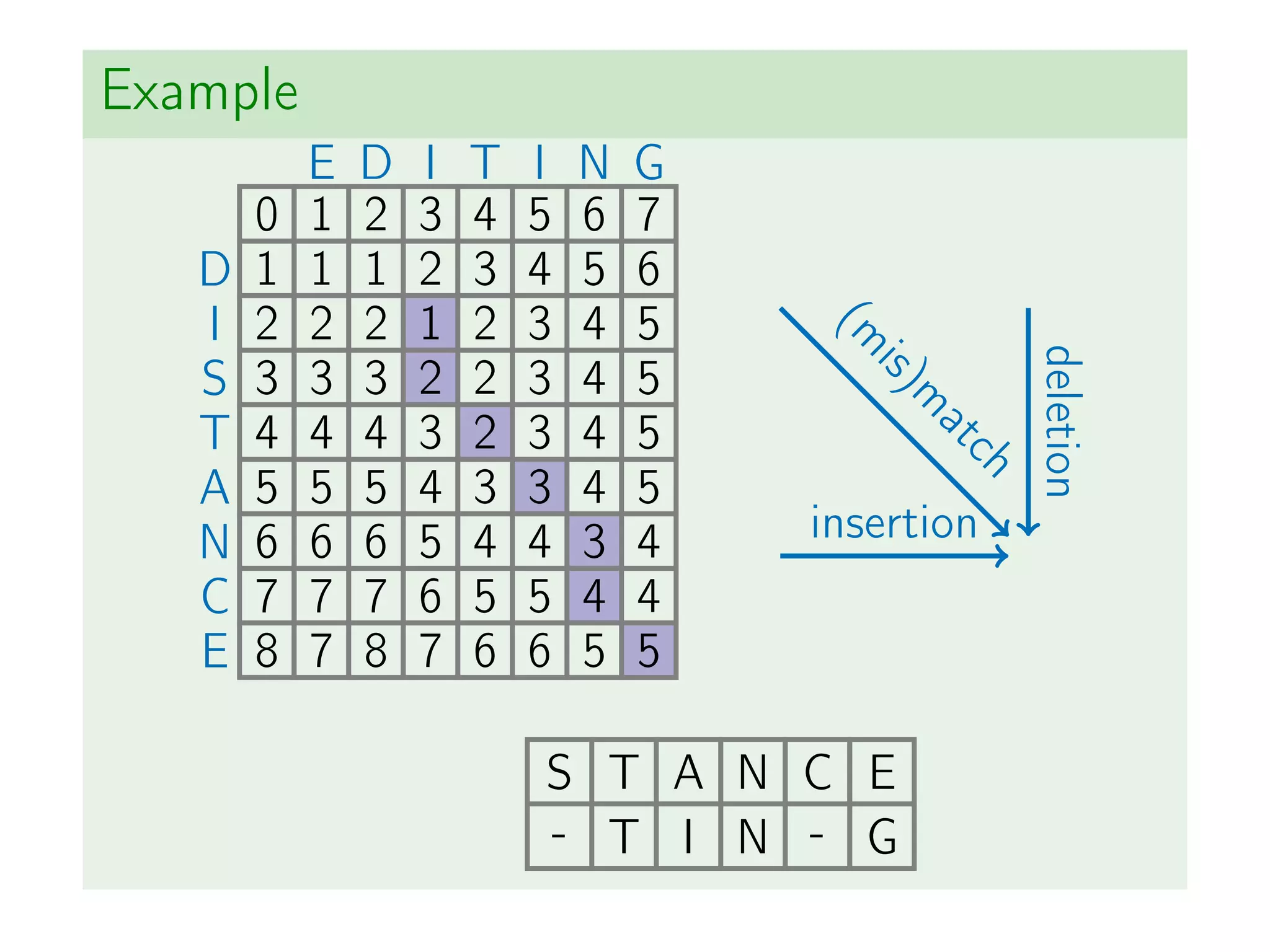
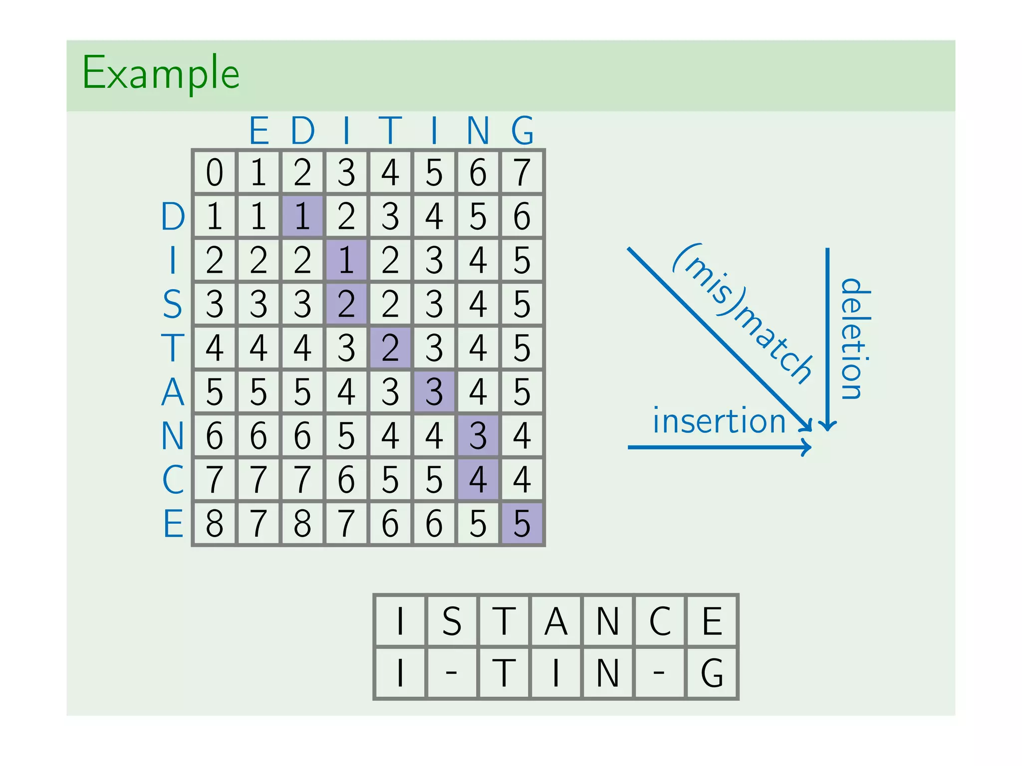
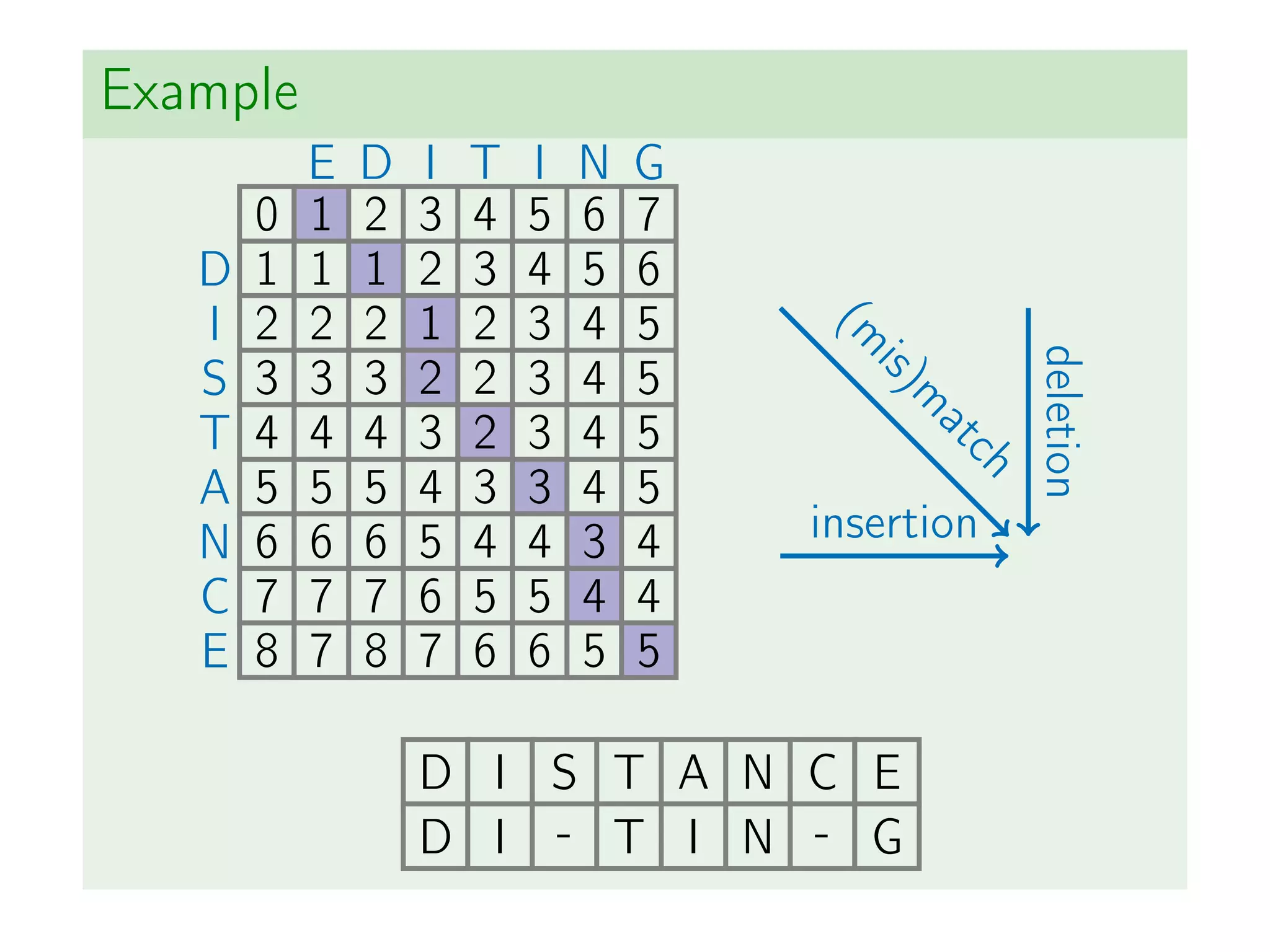
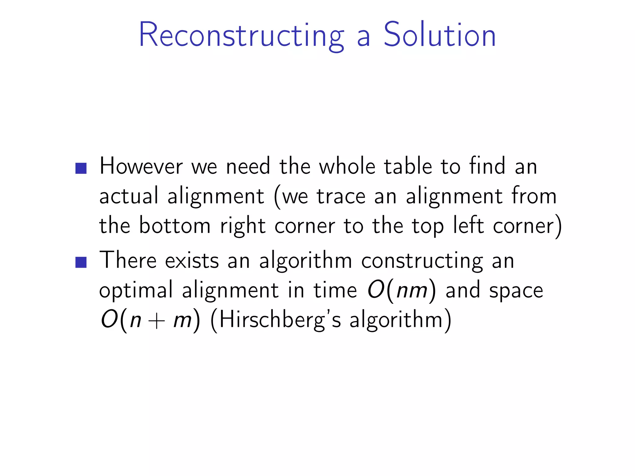
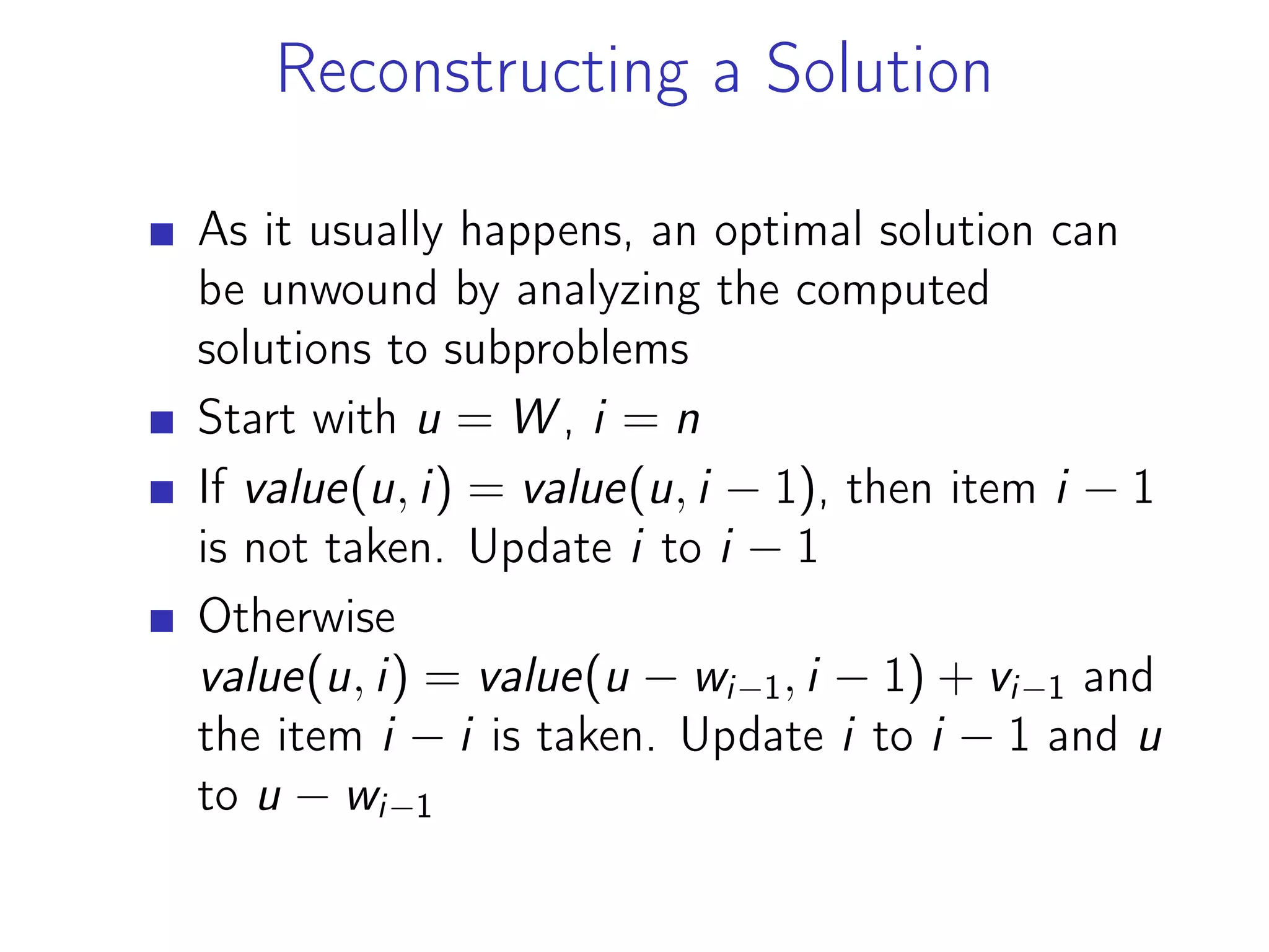
![Reconstructing a Solution
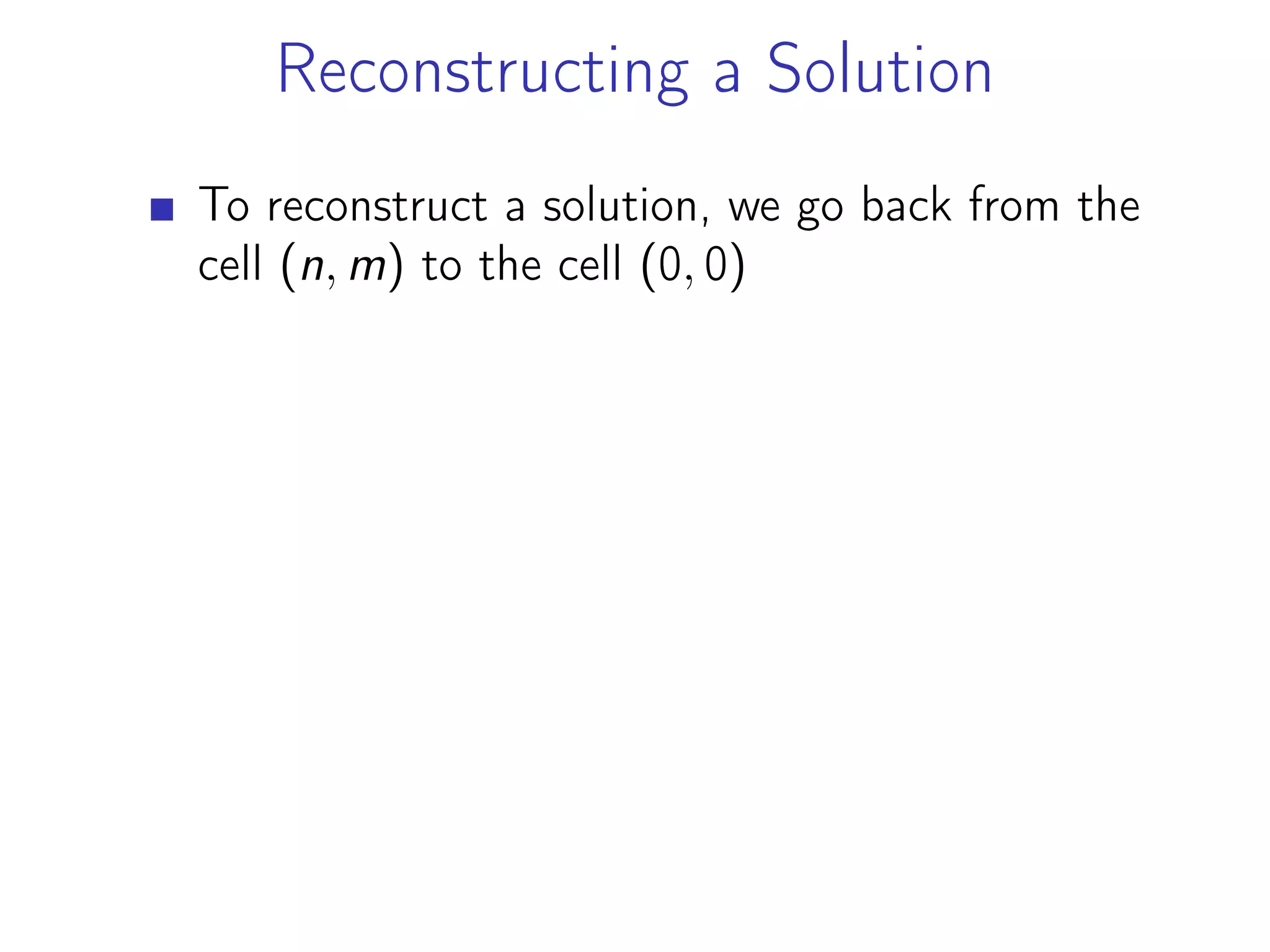
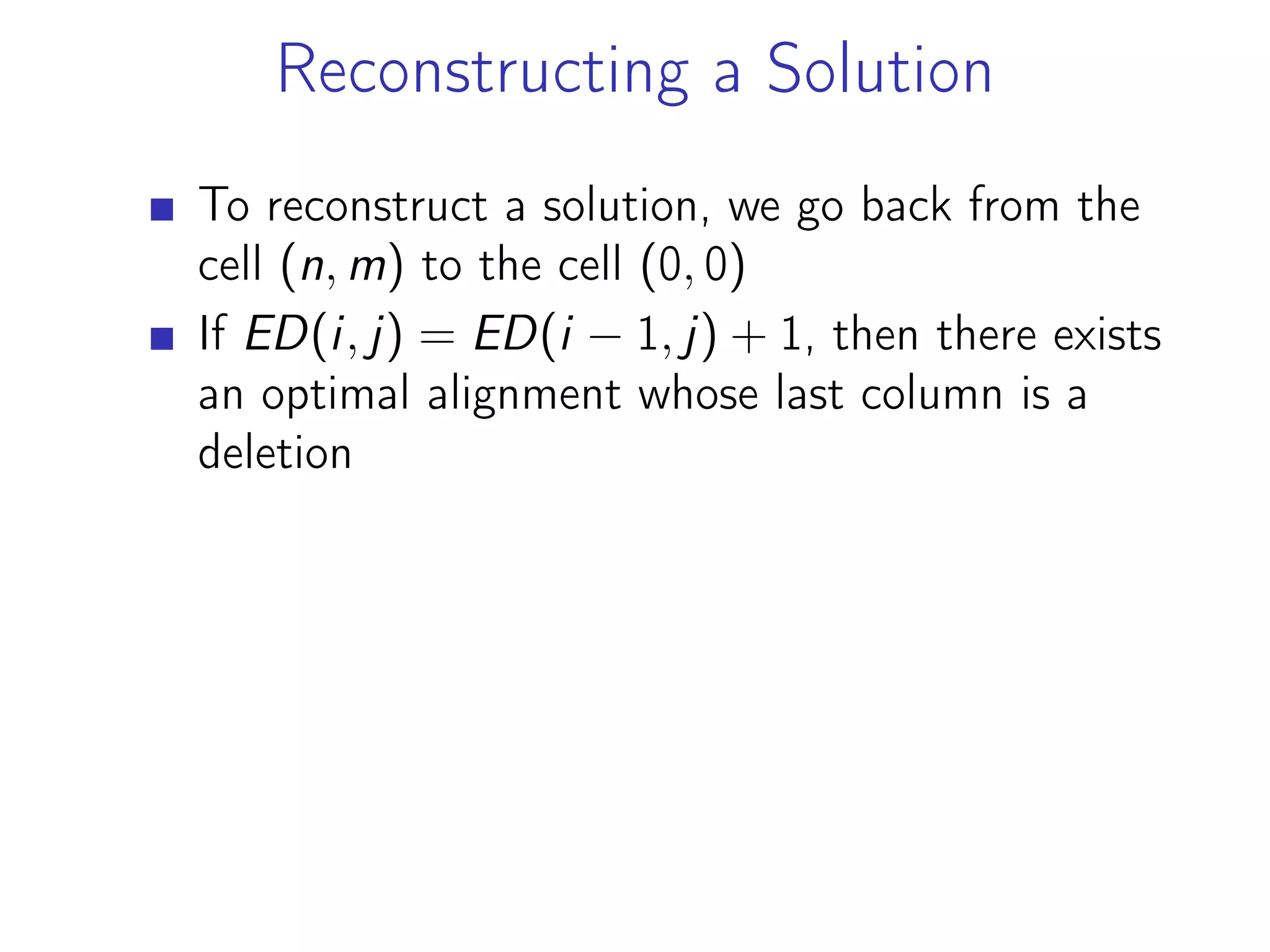
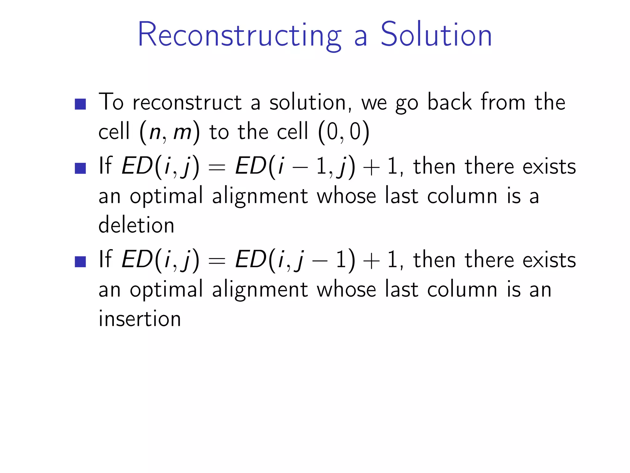
To reconstruct a solution, we go back from the
cell (n, m) to the cell (0, 0)
If ED(i, j) = ED(i − 1, j) + 1, then there exists
an optimal alignment whose last column is a
deletion
If ED(i, j) = ED(i, j − 1) + 1, then there exists
an optimal alignment whose last column is an
insertion
If ED(i, j) = ED(i − 1, j − 1) + diff(A[i], B[j]),
then match (if A[i] = B[j]) or mismatch (if
A[i] ̸= B[j])](https://image.slidesharecdn.com/dynamicprograming-220116082321/75/Dynamic-programing-152-2048.jpg)
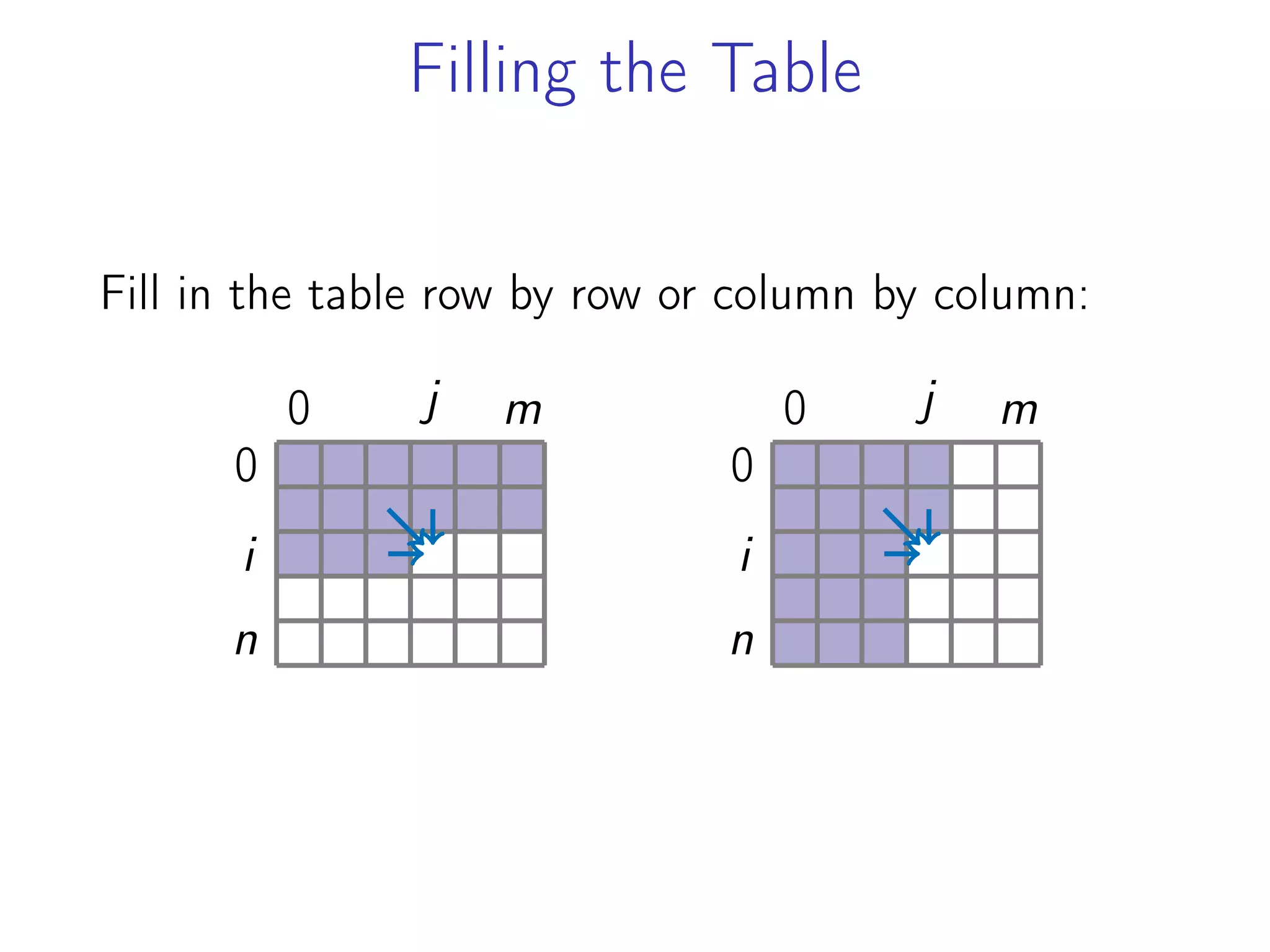
![Saving Space
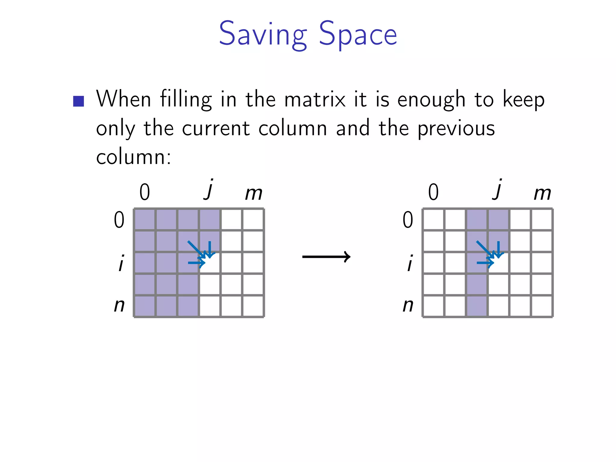
When filling in the matrix it is enough to keep
only the current column and the previous
column:
0
n
i
0 m
j
0
n
i
0 m
j
Thus, one can compute the edit distance of two
given strings A[1 . . . n] and B[1 . . . m] in time
O(nm) and space O(min{n, m}).](https://image.slidesharecdn.com/dynamicprograming-220116082321/75/Dynamic-programing-165-2048.jpg)
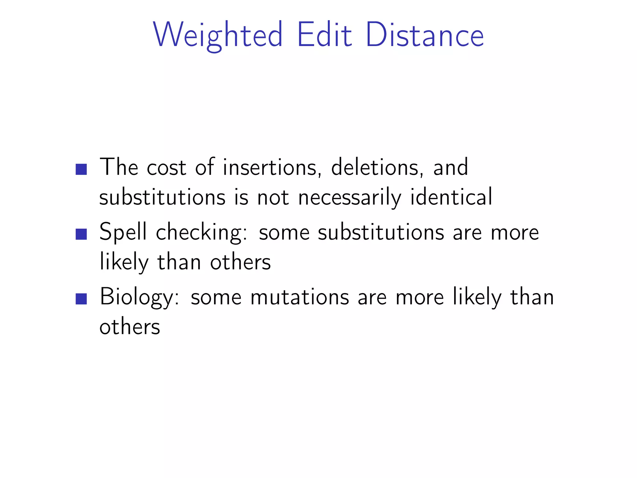
![Generalized Recurrence Relation
min
⎧
⎪
⎨
⎪
⎩
ED(i, j − 1) + inscost(B[j]),
ED(i − 1, j) + delcost(A[i]),
ED(i − 1, j − 1) + substcost(A[i], B[j])](https://image.slidesharecdn.com/dynamicprograming-220116082321/75/Dynamic-programing-169-2048.jpg)
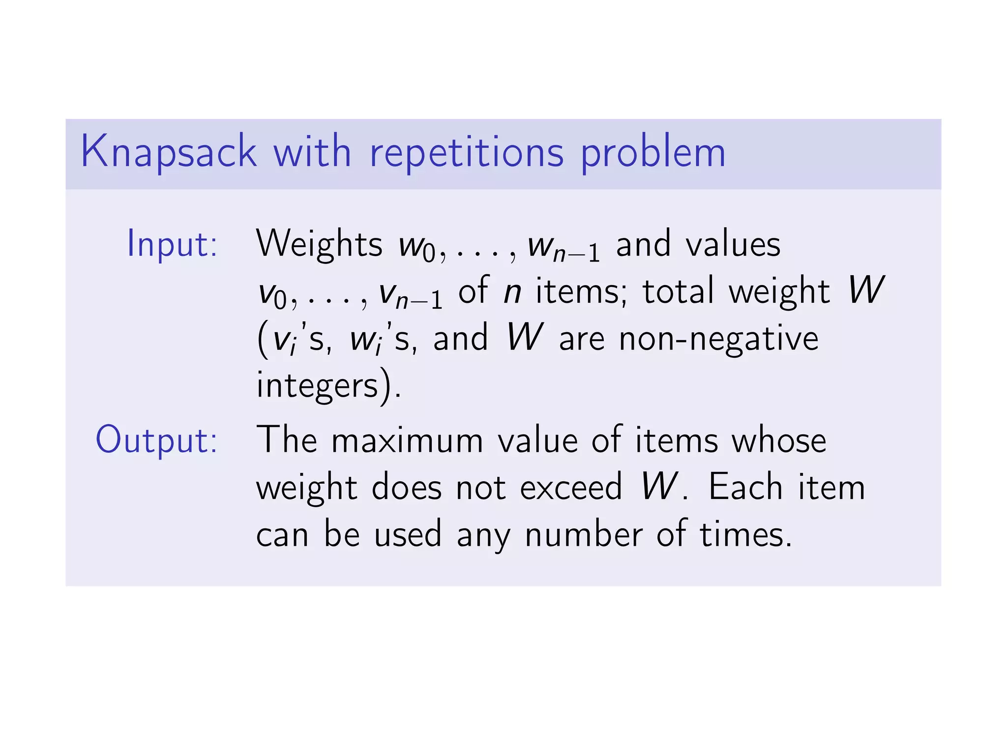
![Recursive Algorithm
1 T = dict ()
2
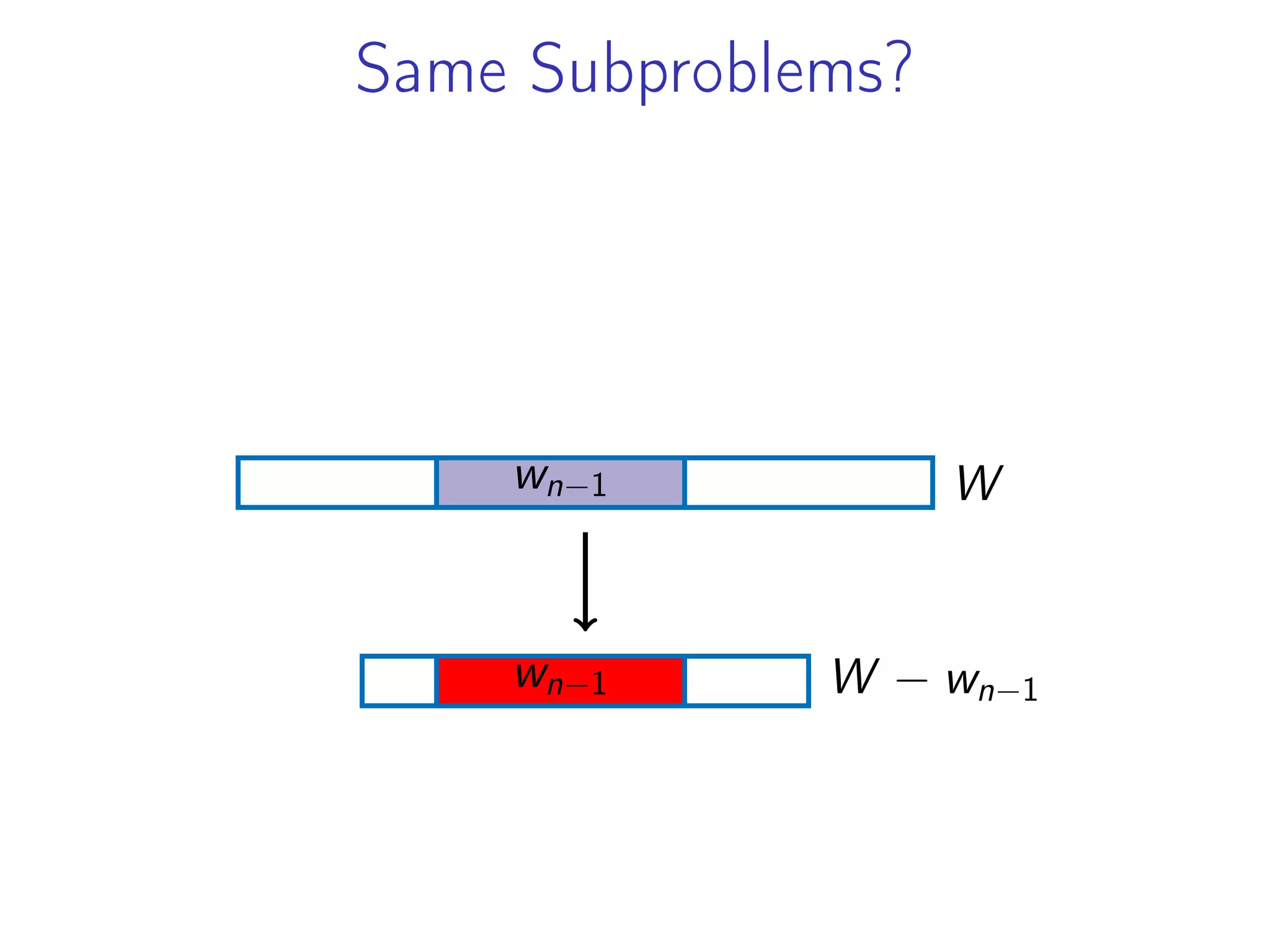
3 def knapsack (w, v , u ) :
4 i f u not in T:
5 T[ u ] = 0
6
7 for i in range ( len (w) ) :
8 i f w[ i ] <= u :
9 T[ u ] = max(T[ u ] ,
10 knapsack (w, v , u − w[ i ] ) + v [ i ] )
11
12 return T[ u ]
13
14
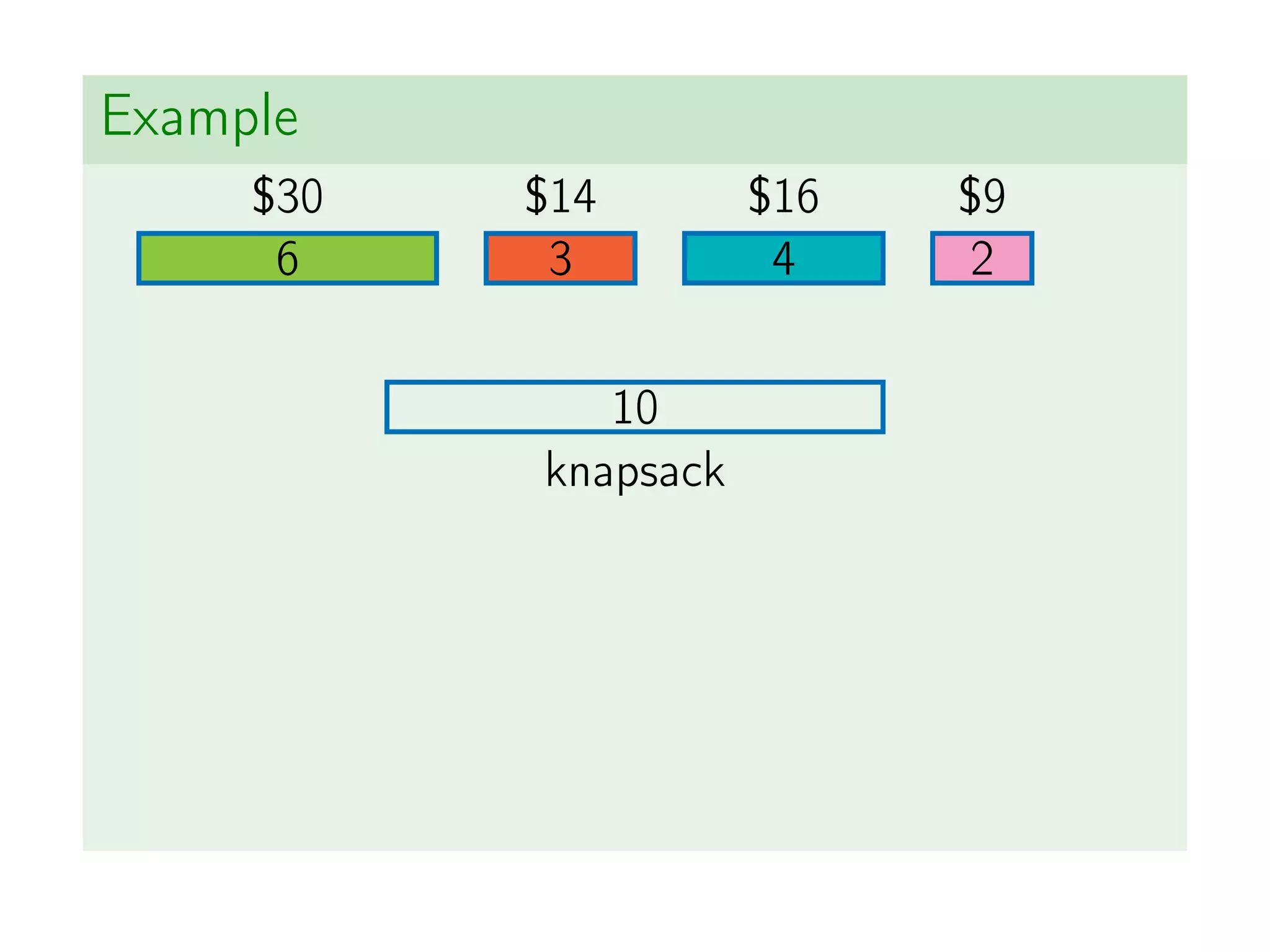
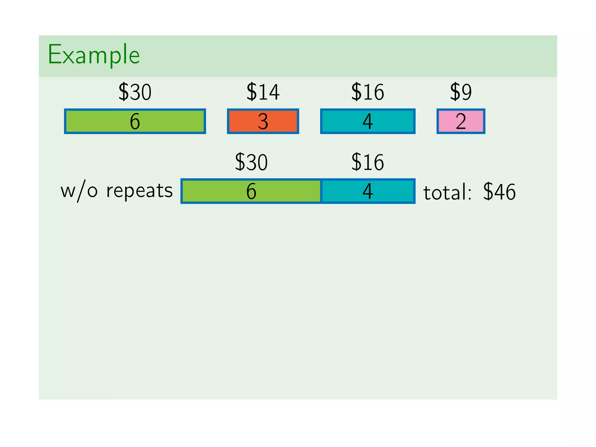
15 print ( knapsack (w=[6 , 3 , 4 , 2] ,
16 v =[30 , 14 , 16 , 9] , u=10))](https://image.slidesharecdn.com/dynamicprograming-220116082321/75/Dynamic-programing-194-2048.jpg)
![Recursive into Iterative
As usual, one can transform a recursive
algorithm into an iterative one
For this, we gradually fill in an array T:
T[u] = value(u)](https://image.slidesharecdn.com/dynamicprograming-220116082321/75/Dynamic-programing-196-2048.jpg)
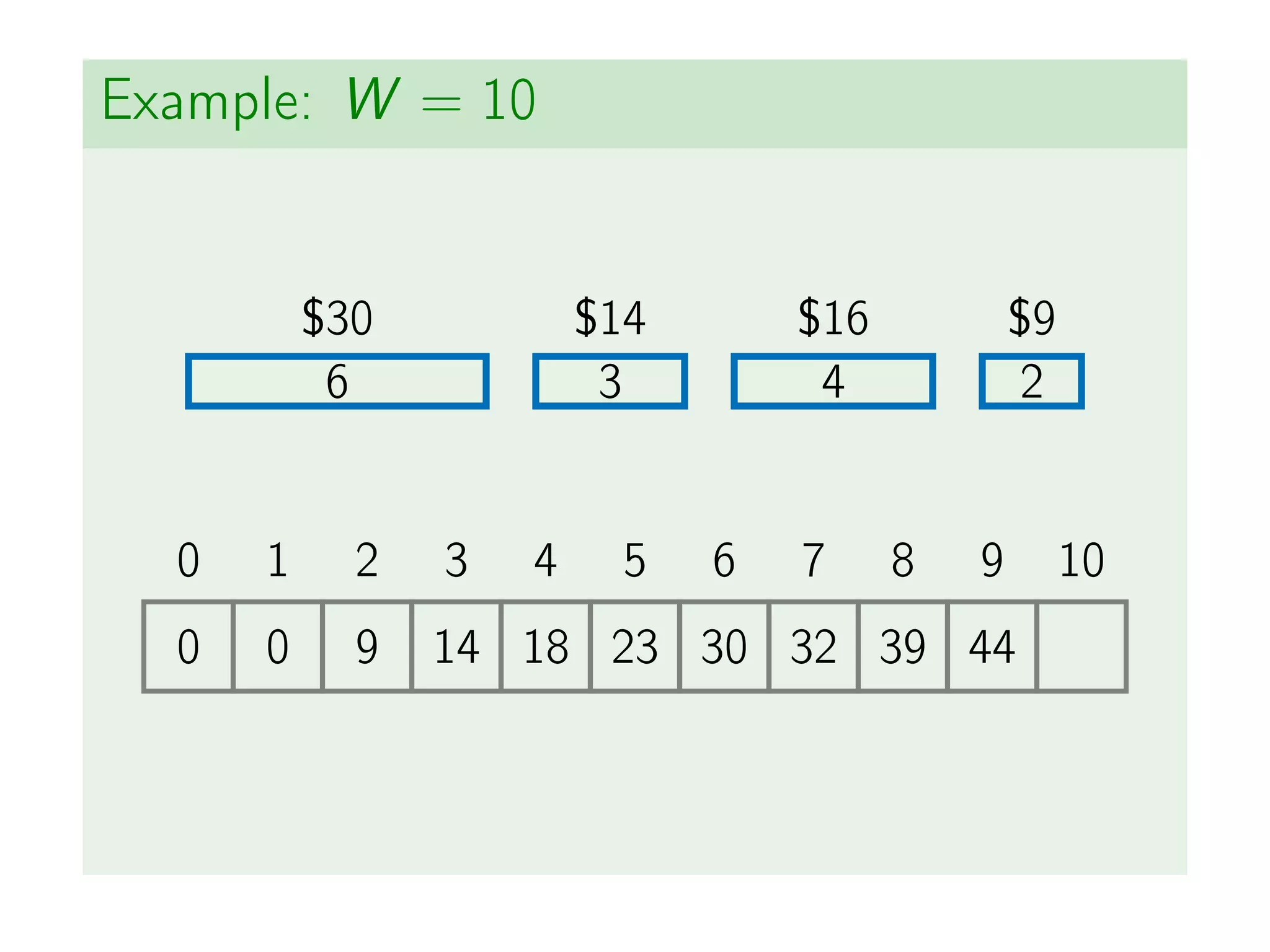
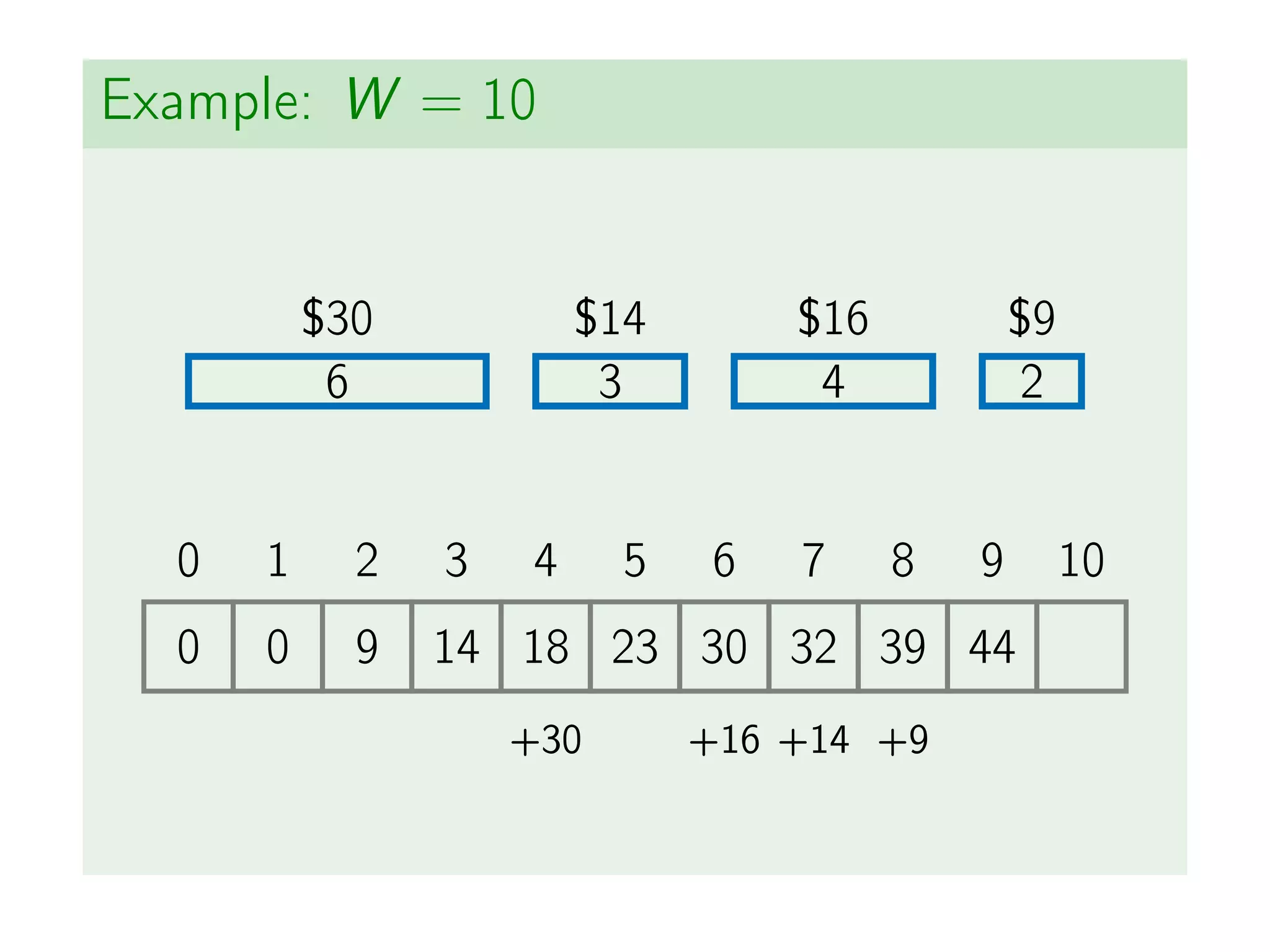
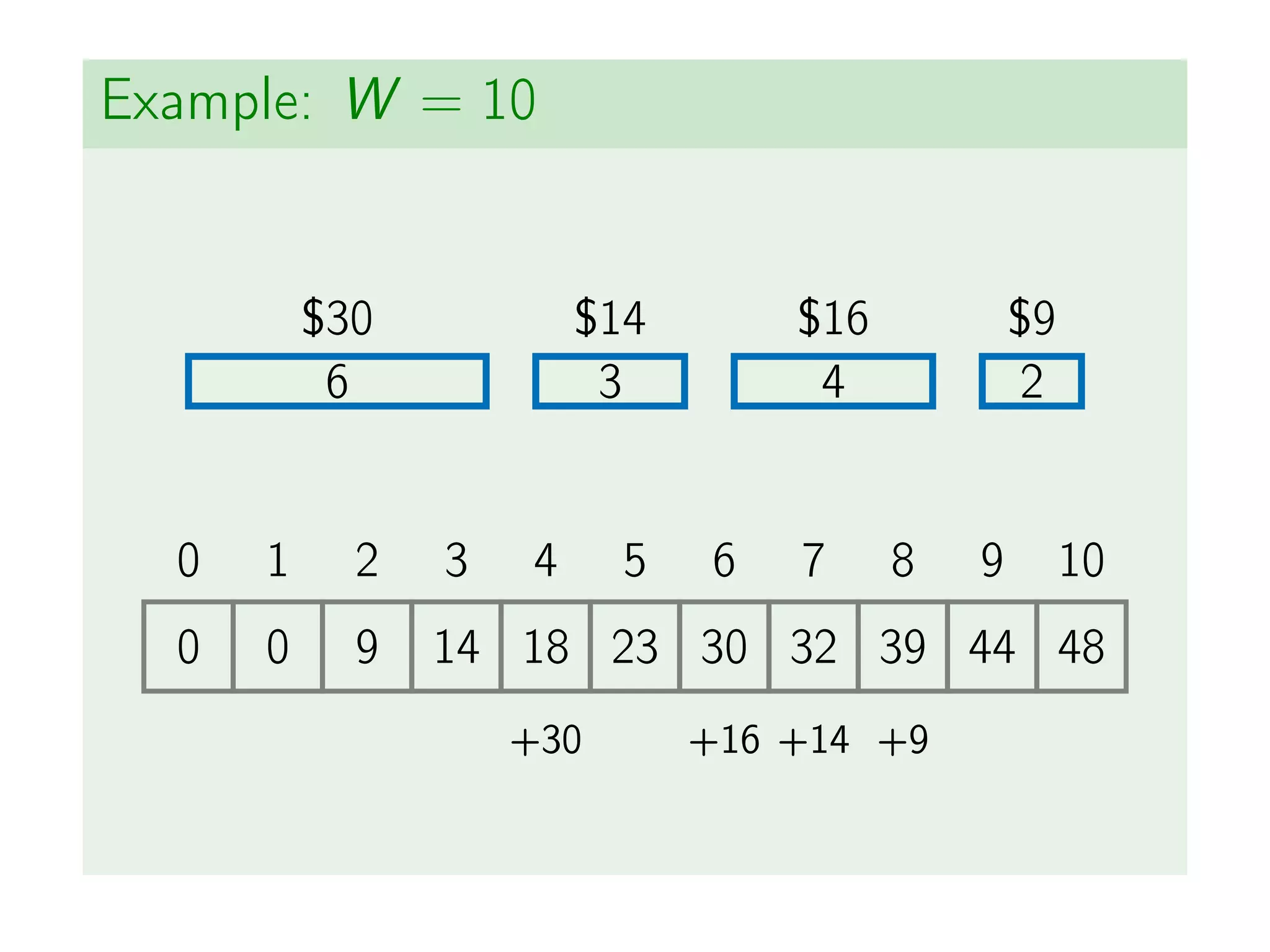
![Recursive Algorithm
1 def knapsack (W, w, v ) :
2 T = [ 0 ] * (W + 1)
3
4 for u in range (1 , W + 1 ) :
5 for i in range ( len (w) ) :
6 i f w[ i ] <= u :
7 T[ u ] = max(T[ u ] , T[ u − w[ i ] ] + v [ i ] )
8
9 return T[W]
10
11
12 print ( knapsack (W=10, w=[6 , 3 , 4 , 2] ,
13 v =[30 , 14 , 16 , 9 ] ) )](https://image.slidesharecdn.com/dynamicprograming-220116082321/75/Dynamic-programing-197-2048.jpg)
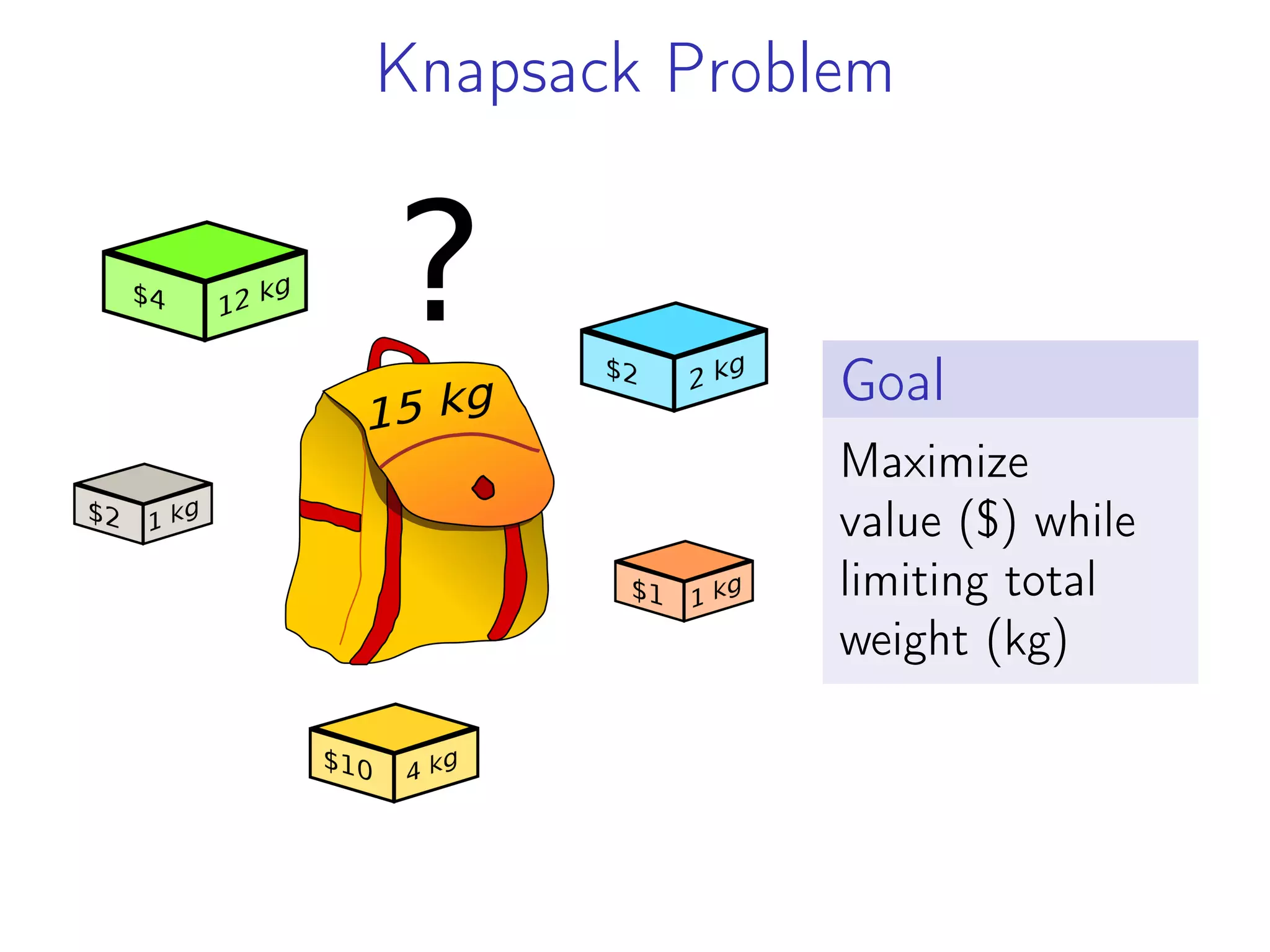
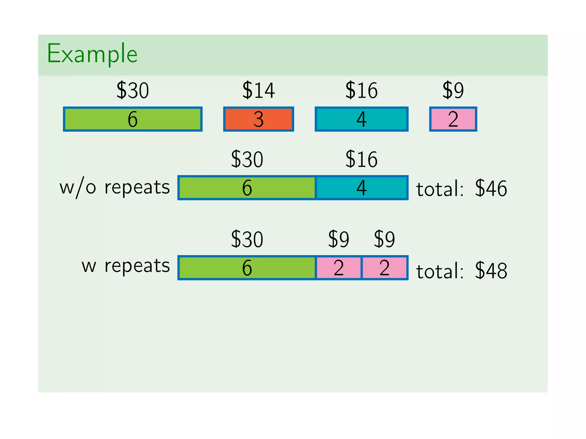
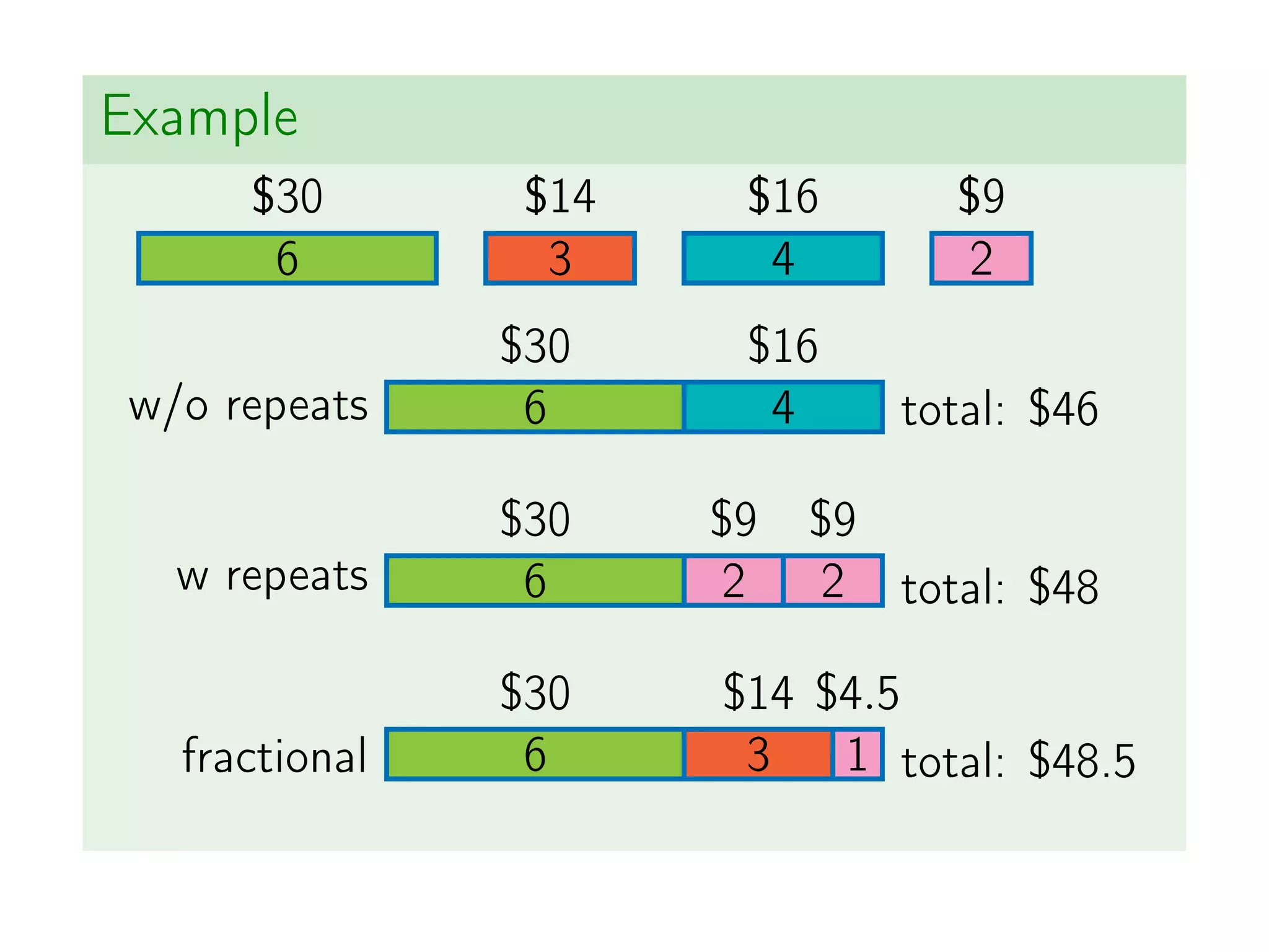
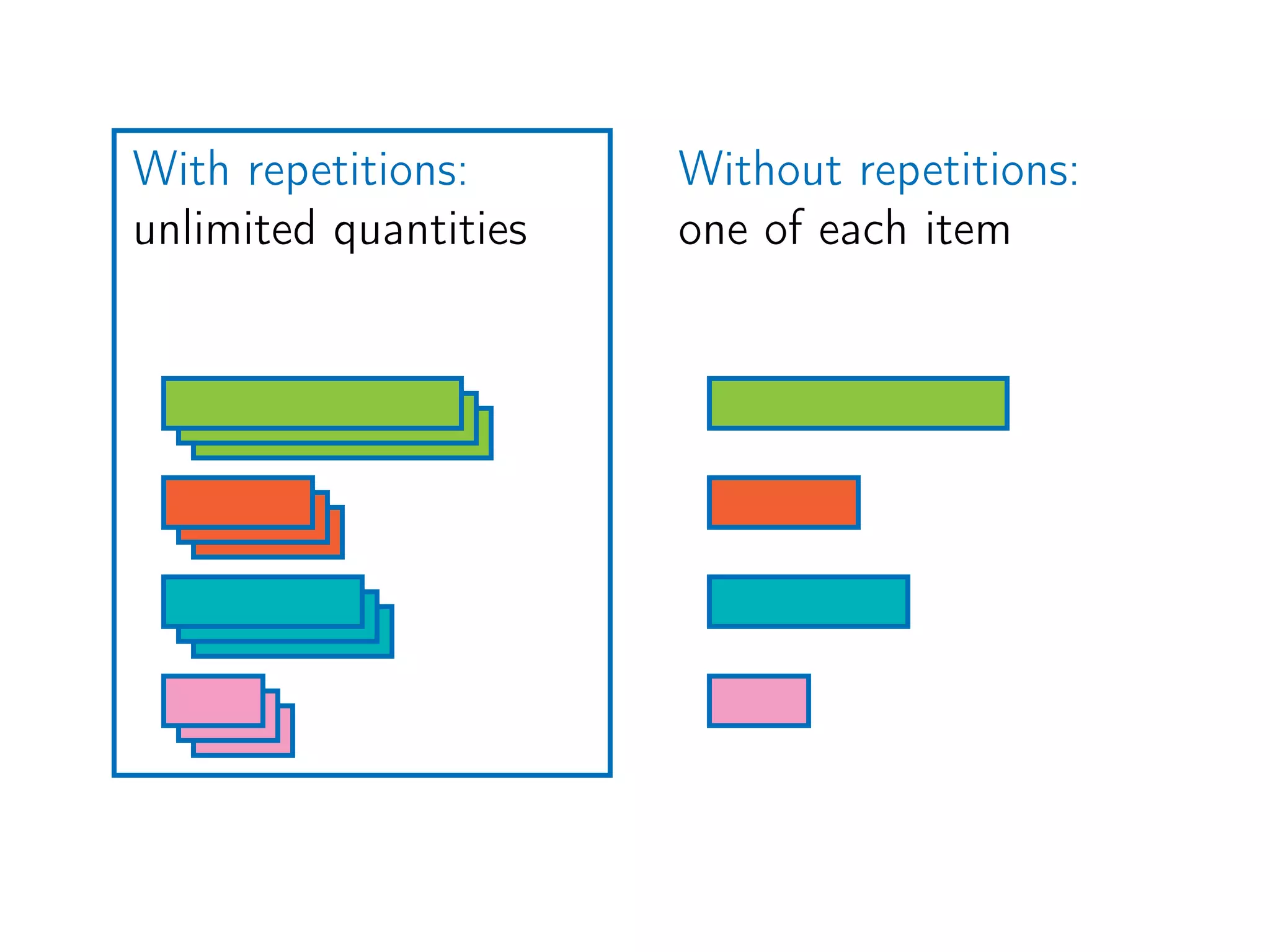
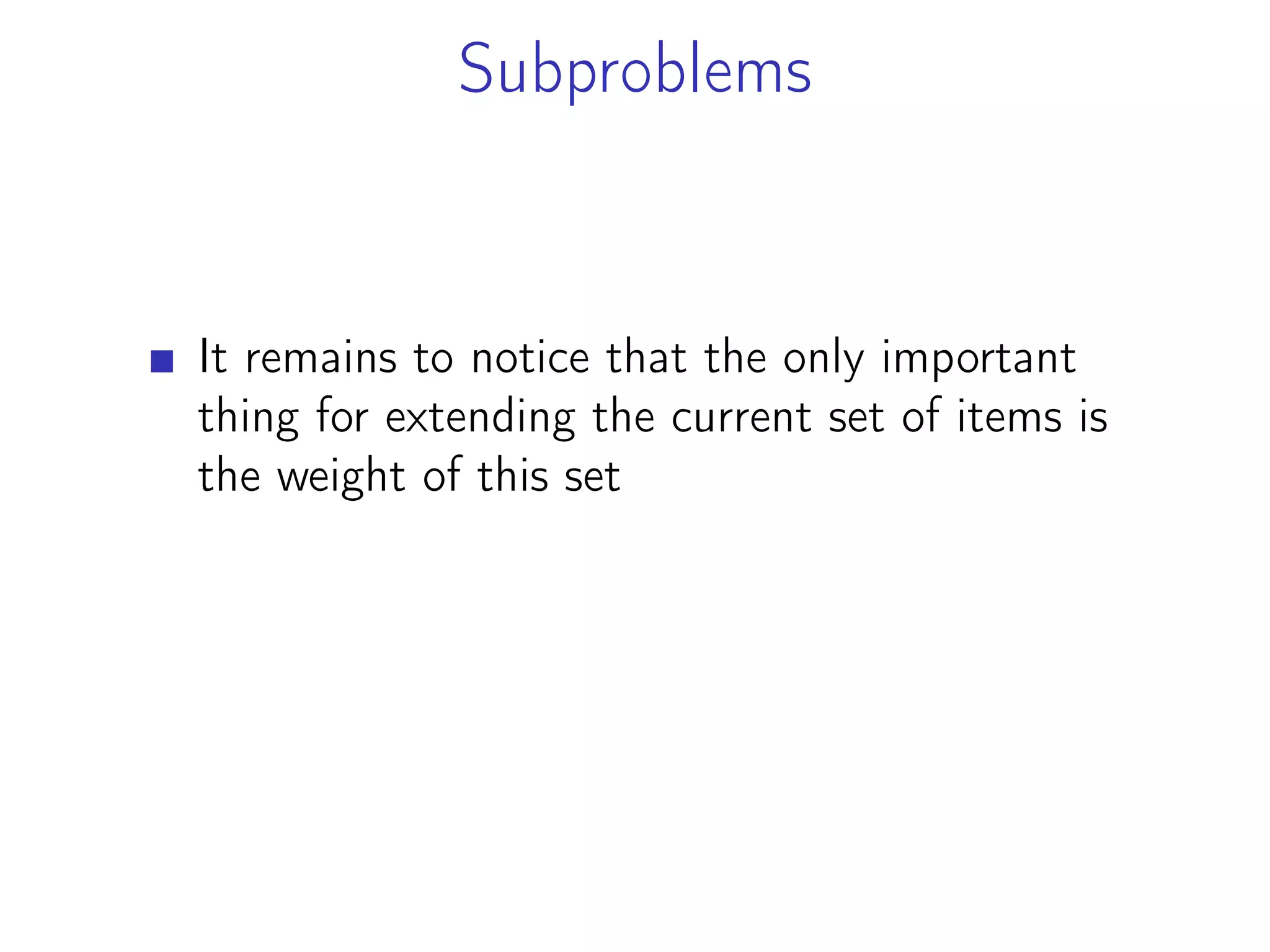
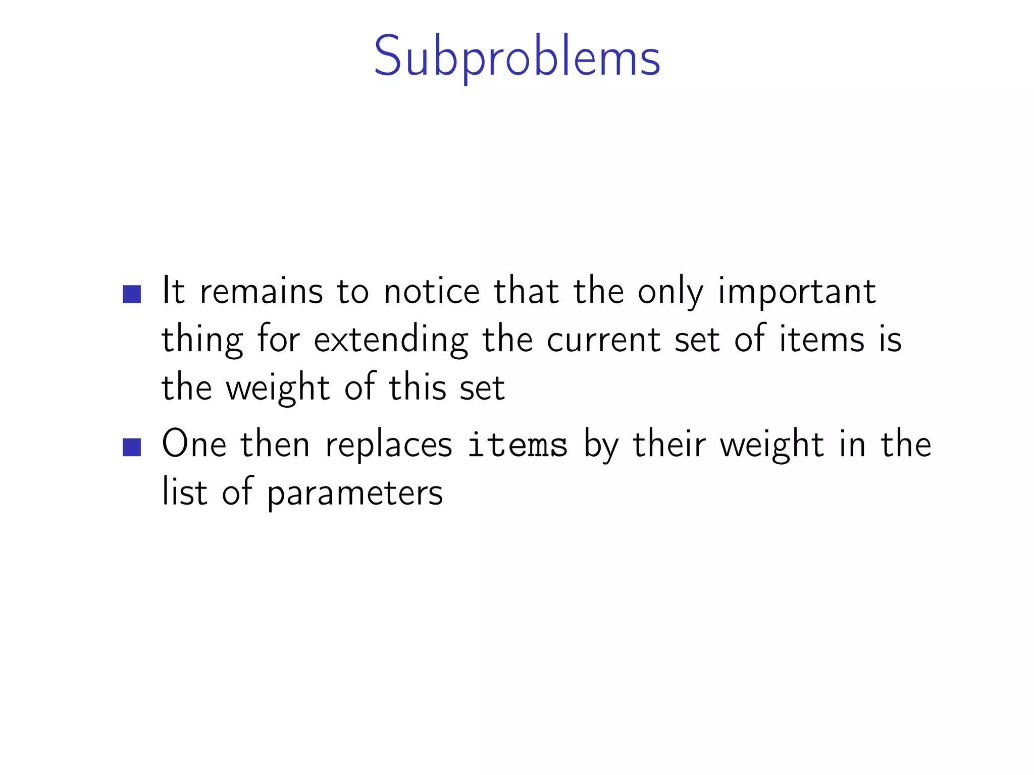
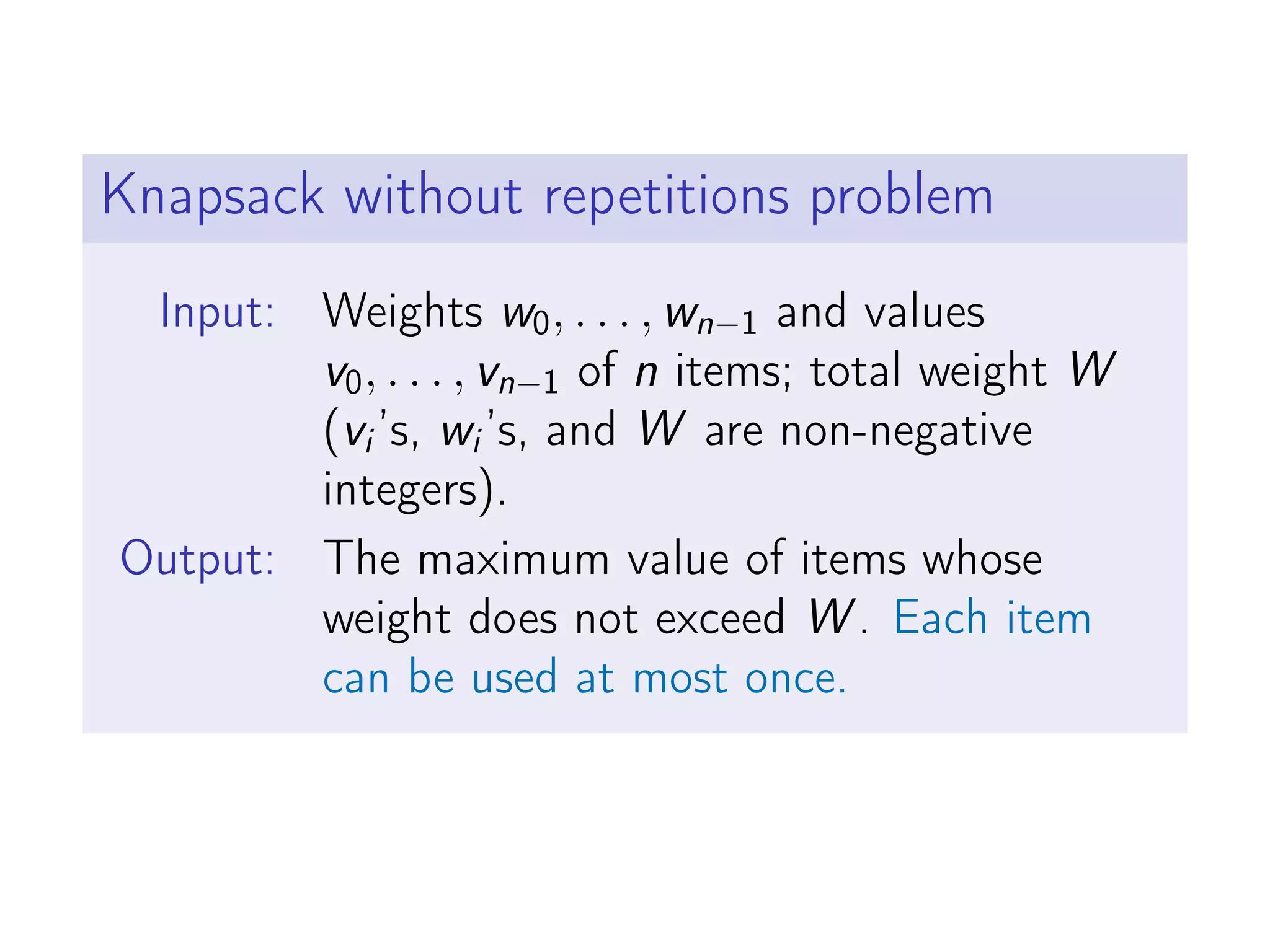
![Brute Force: Knapsack with Repetitions
1 def knapsack (W, w, v , items ) :
2 weight = sum(w[ i ] for i in items )
3 value = sum( v [ i ] for i in items )
4
5 for i in range ( len (w) ) :
6 i f weight + w[ i ] <= W:
7 value = max( value ,
8 knapsack (W, w, v , items + [ i ] ) )
9
10 return value
11
12 print ( knapsack (W=10, w=[6 , 3 , 4 , 2] ,
13 v =[30 , 14 , 16 , 9] , items =[]))](https://image.slidesharecdn.com/dynamicprograming-220116082321/75/Dynamic-programing-203-2048.jpg)
![Recursive Algorithm
1 T = dict ()
2
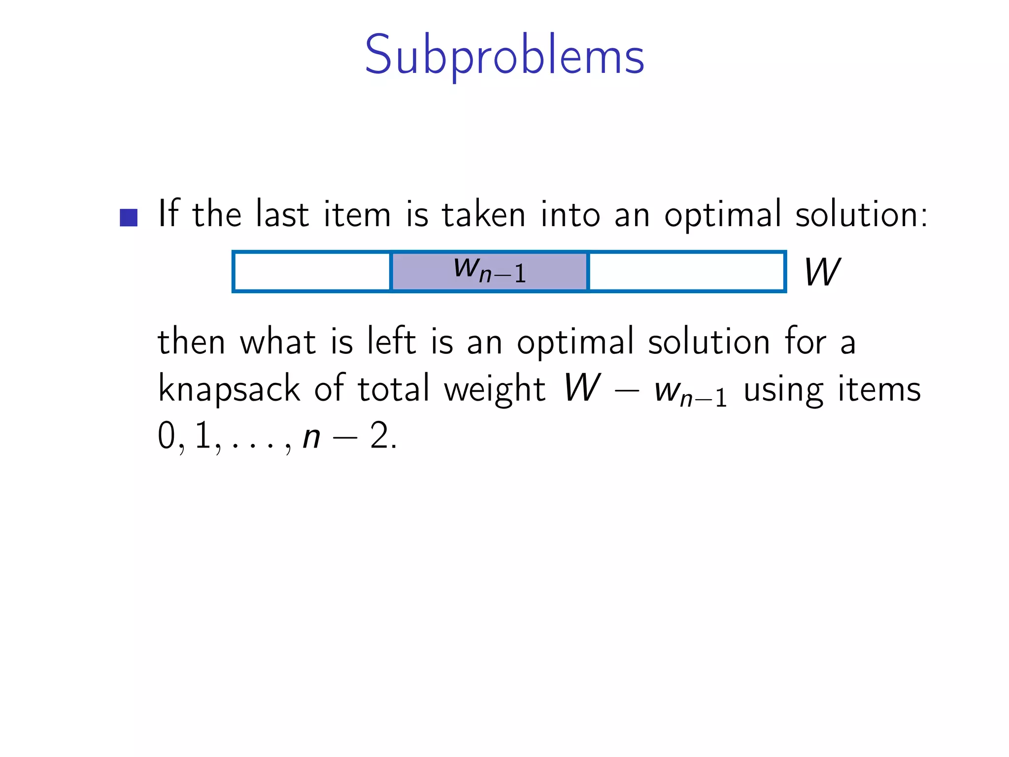
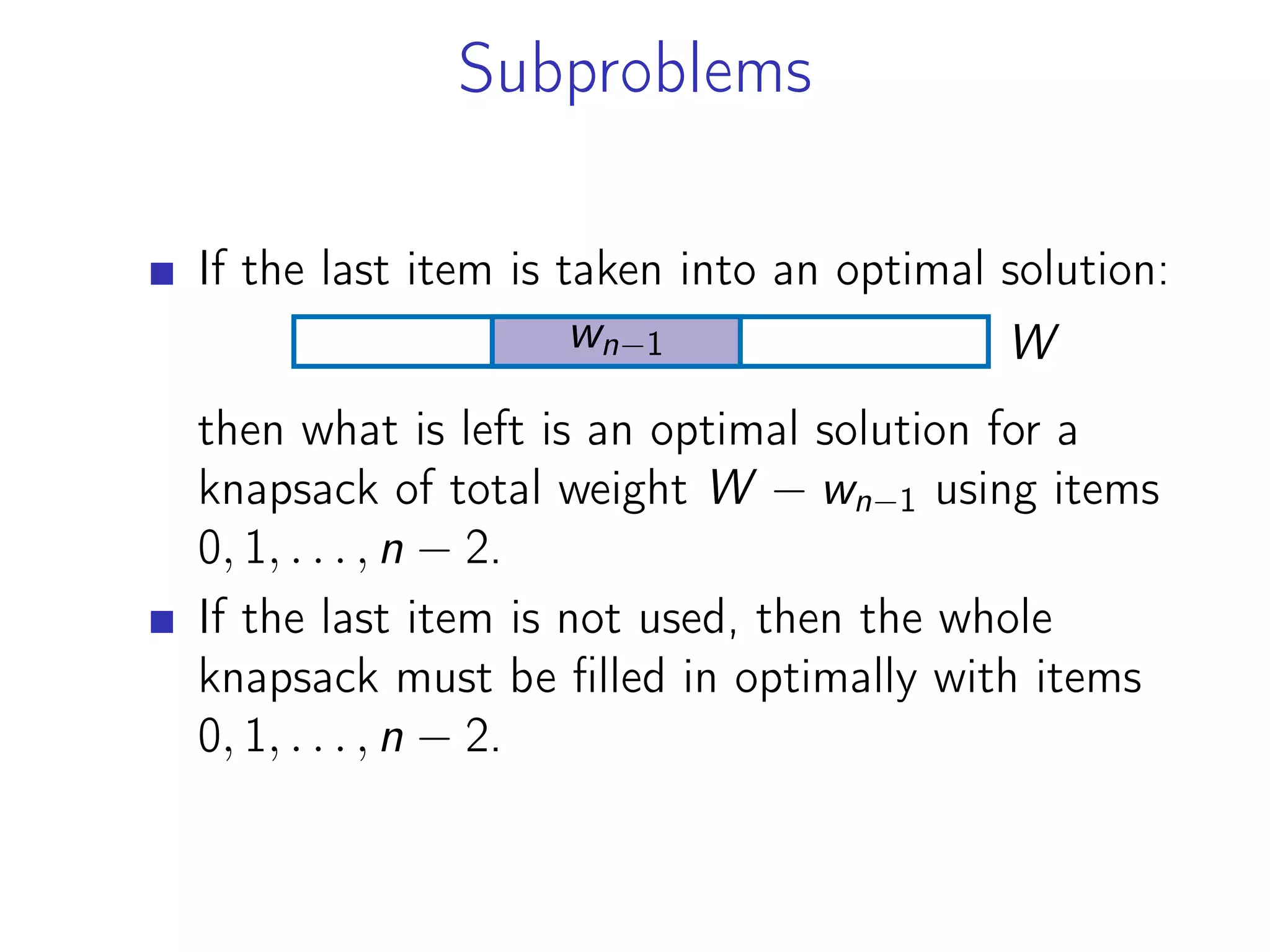
3 def knapsack (w, v , u , i ) :
4 i f (u , i ) not in T:
5 i f i == 0:
6 T[ u , i ] = 0
7 else :
8 T[ u , i ] = knapsack (w, v , u , i − 1)
9 i f u >= w[ i − 1 ] :
10 T[ u , i ] = max(T[ u , i ] ,
11 knapsack (w, v , u − w[ i − 1] , i − 1) + v [ i − 1 ]
12
13 return T[ u , i ]
14
15
16 print ( knapsack (w=[6 , 3 , 4 , 2] ,
17 v =[30 , 14 , 16 , 9] , u=10, i =4))](https://image.slidesharecdn.com/dynamicprograming-220116082321/75/Dynamic-programing-218-2048.jpg)
![Iterative Algorithm
1 def knapsack (W, w, v ) :
2 T = [ [ None ] * ( len (w) + 1) for _ in range (W + 1 ) ]
3
4 for u in range (W + 1 ) :
5 T[ u ] [ 0 ] = 0
6
7 for i in range (1 , len (w) + 1 ) :
8 for u in range (W + 1 ) :
9 T[ u ] [ i ] = T[ u ] [ i − 1]
10 i f u >= w[ i − 1 ] :
11 T[ u ] [ i ] = max(T[ u ] [ i ] ,
12 T[ u − w[ i − 1 ] ] [ i − 1] + v [ i − 1 ] )
13
14 return T[W] [ len (w) ]
15
16
17 print ( knapsack (W=10, w=[6 , 3 , 4 , 2] ,
18 v =[30 , 14 , 16 , 9 ] ) )](https://image.slidesharecdn.com/dynamicprograming-220116082321/75/Dynamic-programing-219-2048.jpg)
![1 def knapsack (W, w, v , items , l a s t ) :
2 weight = sum(w[ i ] for i in items )
3
4 i f l a s t == len (w) − 1:
5 return sum( v [ i ] for i in items )
6
7 value = knapsack (W, w, v , items , l a s t + 1)
8 i f weight + w[ l a s t + 1] <= W:
9 items . append ( l a s t + 1)
10 value = max( value ,
11 knapsack (W, w, v , items , l a s t + 1))
12 items . pop ()
13
14 return value
15
16 print ( knapsack (W=10, w=[6 , 3 , 4 , 2] ,
17 v =[30 , 14 , 16 , 9] ,
18 items =[] , l a s t =−1))](https://image.slidesharecdn.com/dynamicprograming-220116082321/75/Dynamic-programing-229-2048.jpg)
![Recursive Algorithm
1 T = dict ()
2
3 def matrix_mult (m, i , j ) :
4 i f ( i , j ) not in T:
5 i f j == i + 1:
6 T[ i , j ] = 0
7 else :
8 T[ i , j ] = f l o a t ( " i n f " )
9 for k in range ( i + 1 , j ) :
10 T[ i , j ] = min(T[ i , j ] ,
11 matrix_mult (m, i , k ) +
12 matrix_mult (m, k , j ) +
13 m[ i ] * m[ j ] * m[ k ] )
14
15 return T[ i , j ]
16
17 print ( matrix_mult (m=[50 , 20 , 1 , 10 , 100] , i =0, j =4))](https://image.slidesharecdn.com/dynamicprograming-220116082321/75/Dynamic-programing-256-2048.jpg)
![Iterative Algorithm
1 def matrix_mult (m) :
2 n = len (m) − 1
3 T = [ [ f l o a t ( " i n f " ) ] * (n + 1) for _ in range (n + 1 ) ]
4
5 for i in range (n ) :
6 T[ i ] [ i + 1] = 0
7
8 for s in range (2 , n + 1 ) :
9 for i in range (n − s + 1 ) :
10 j = i + s
11 for k in range ( i + 1 , j ) :
12 T[ i ] [ j ] = min(T[ i ] [ j ] ,
13 T[ i ] [ k ] + T[ k ] [ j ] +
14 m[ i ] * m[ j ] * m[ k ] )
15
16 return T [ 0 ] [ n ]
17
18 print ( matrix_mult (m=[50 , 20 , 1 , 10 , 100]))](https://image.slidesharecdn.com/dynamicprograming-220116082321/75/Dynamic-programing-258-2048.jpg)
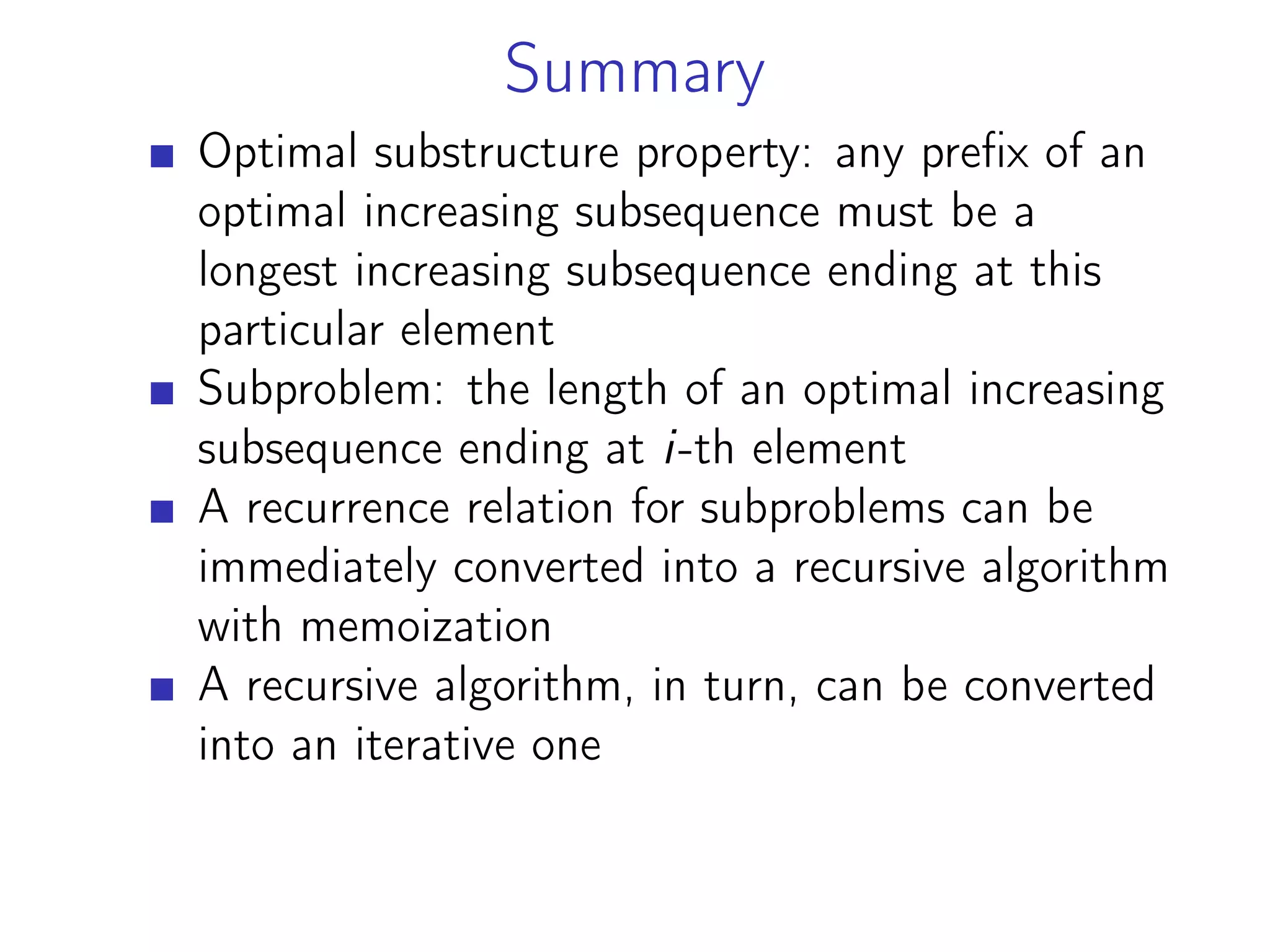
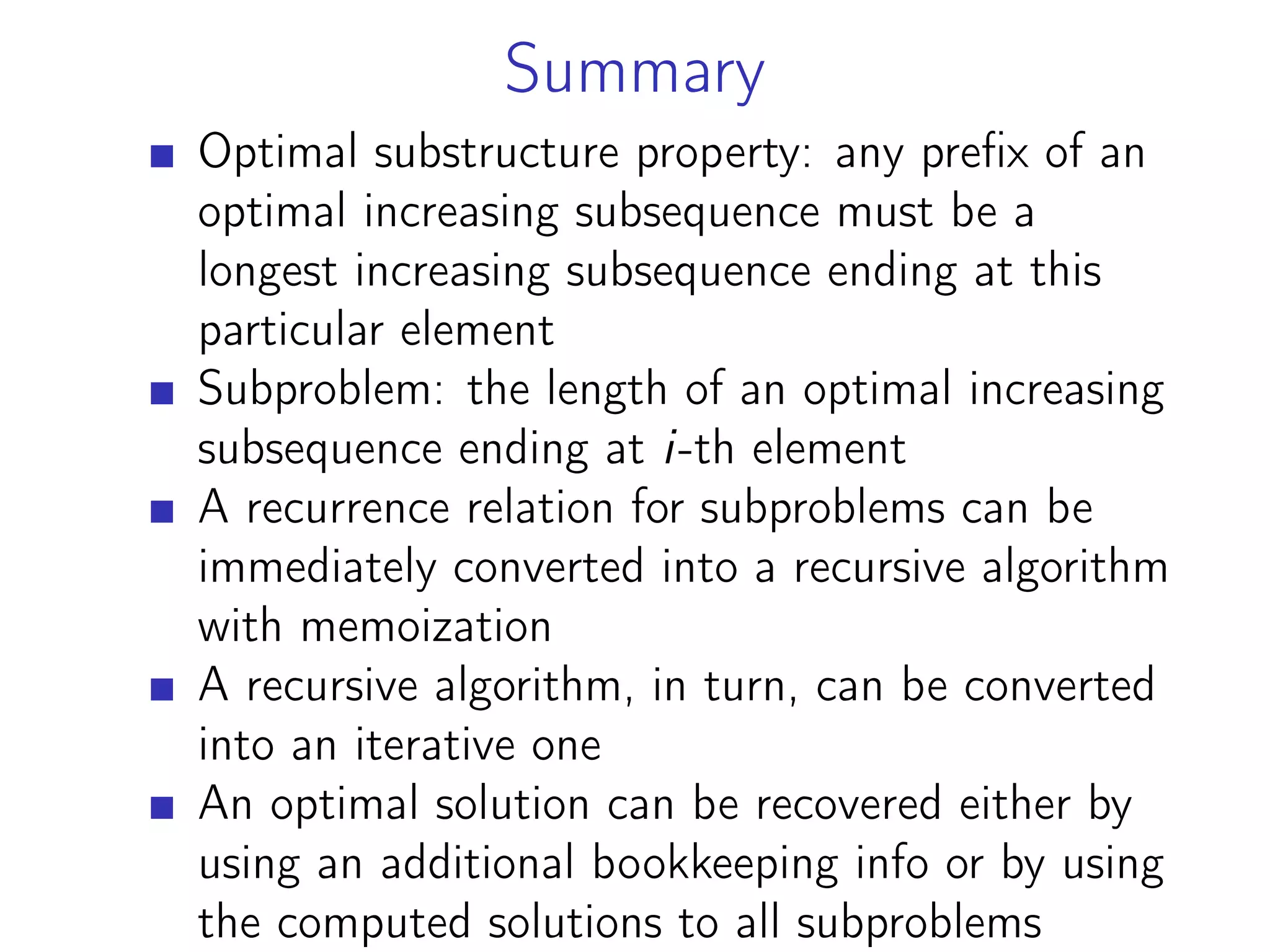
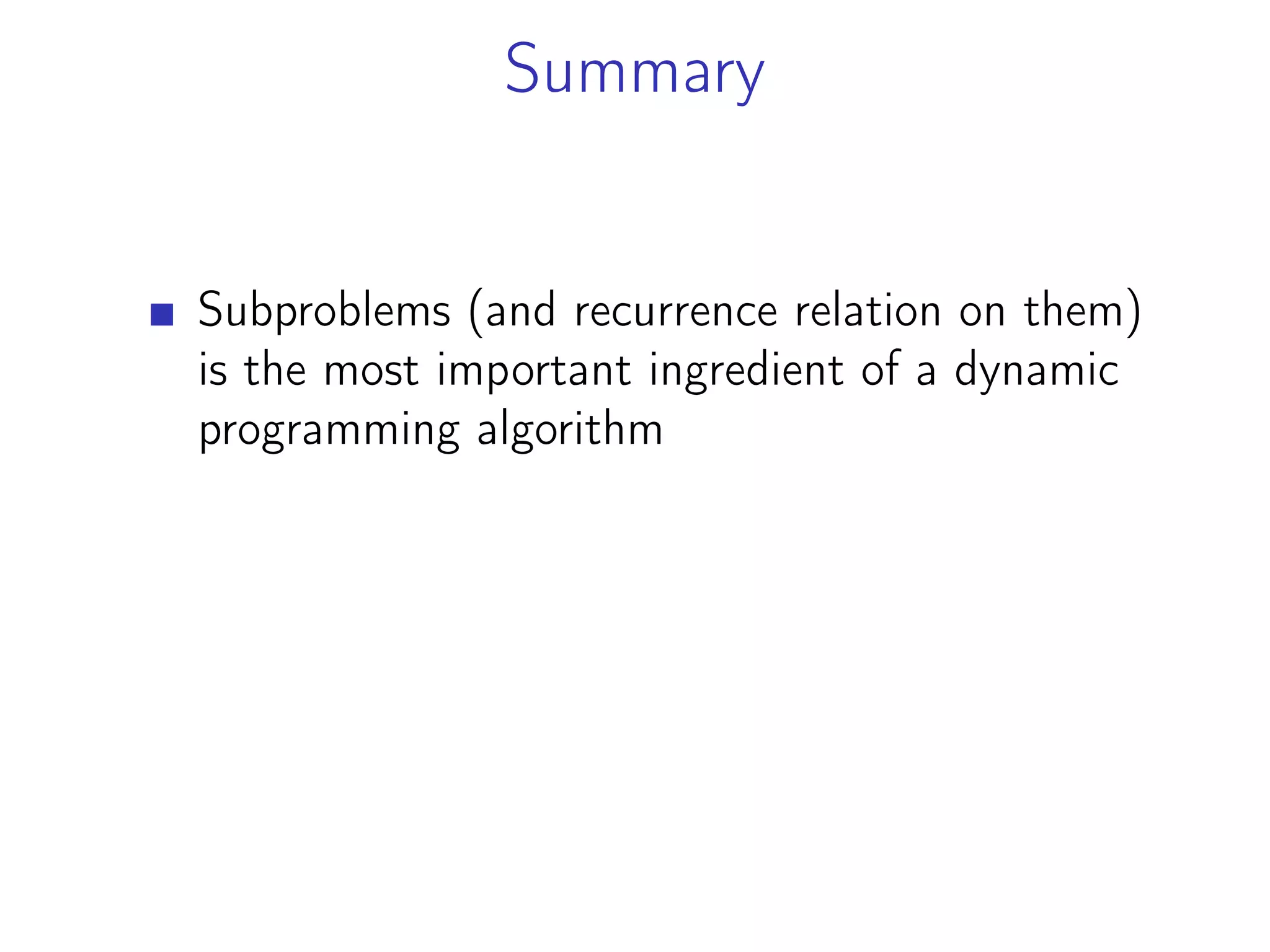
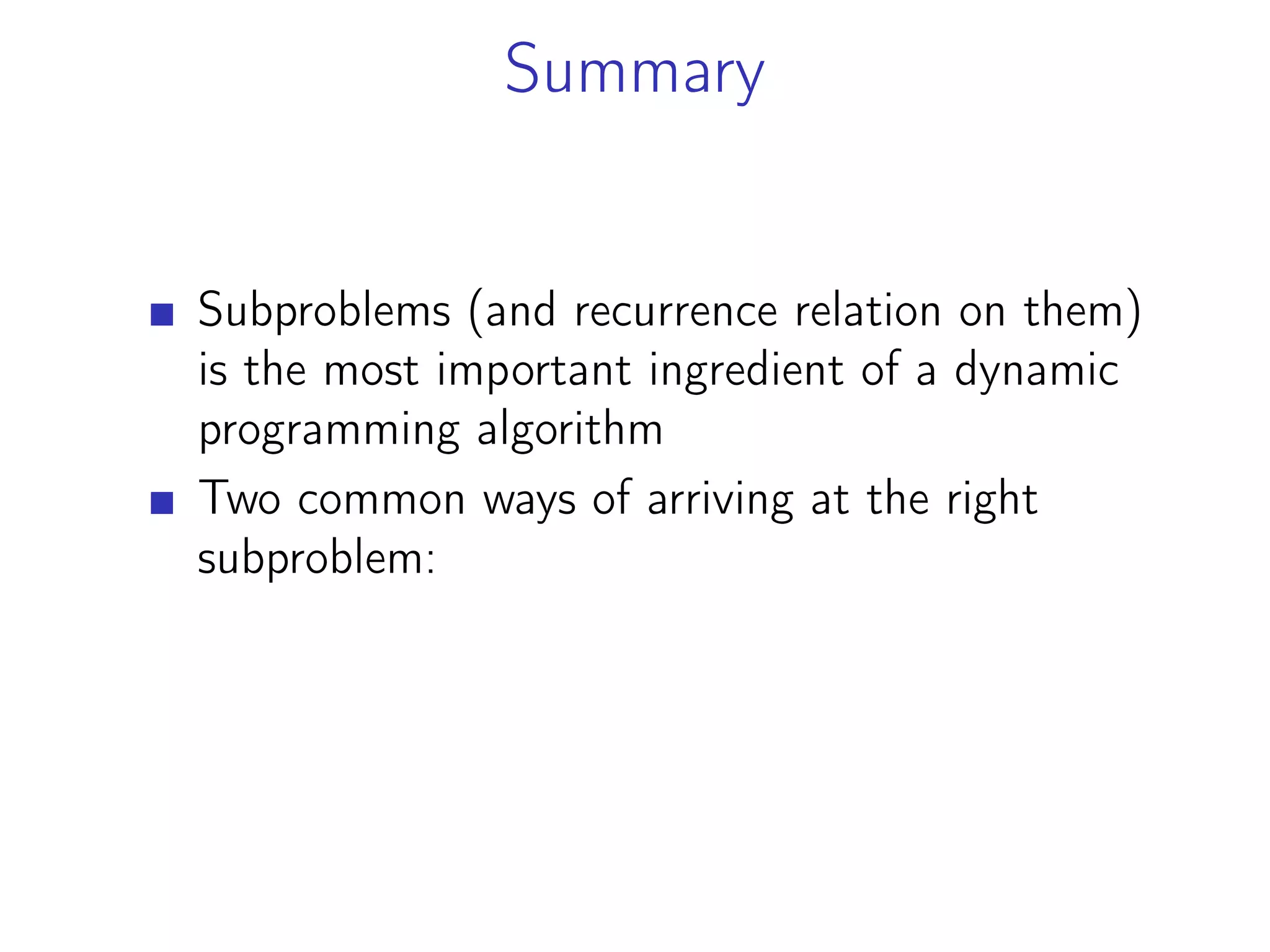
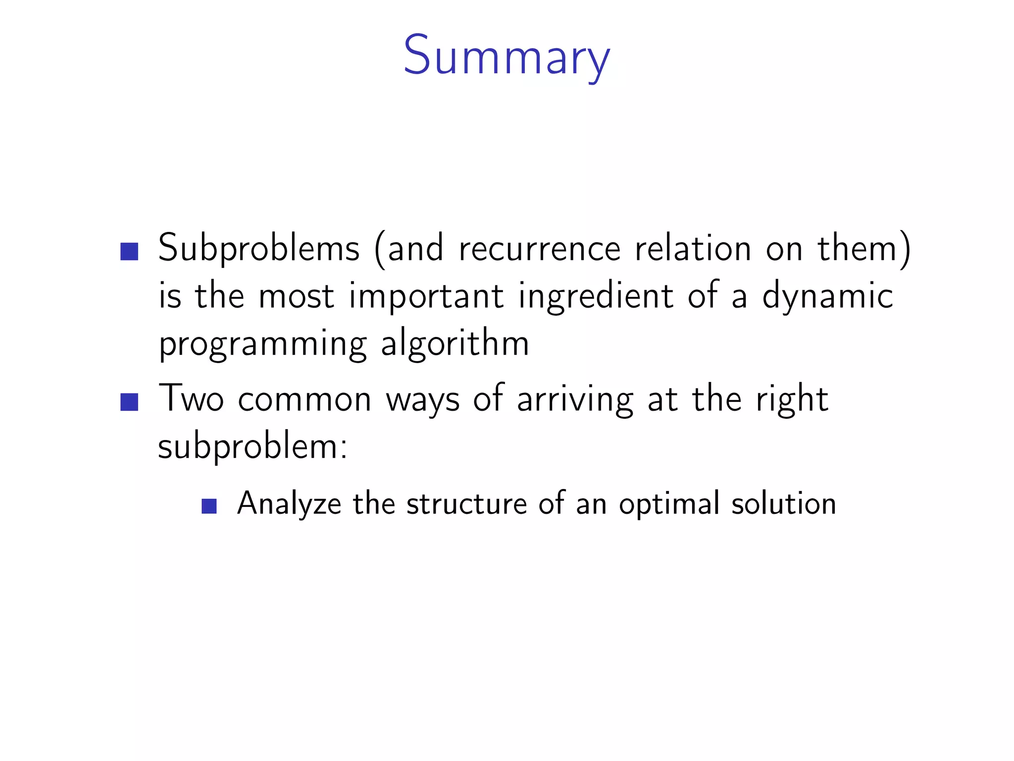
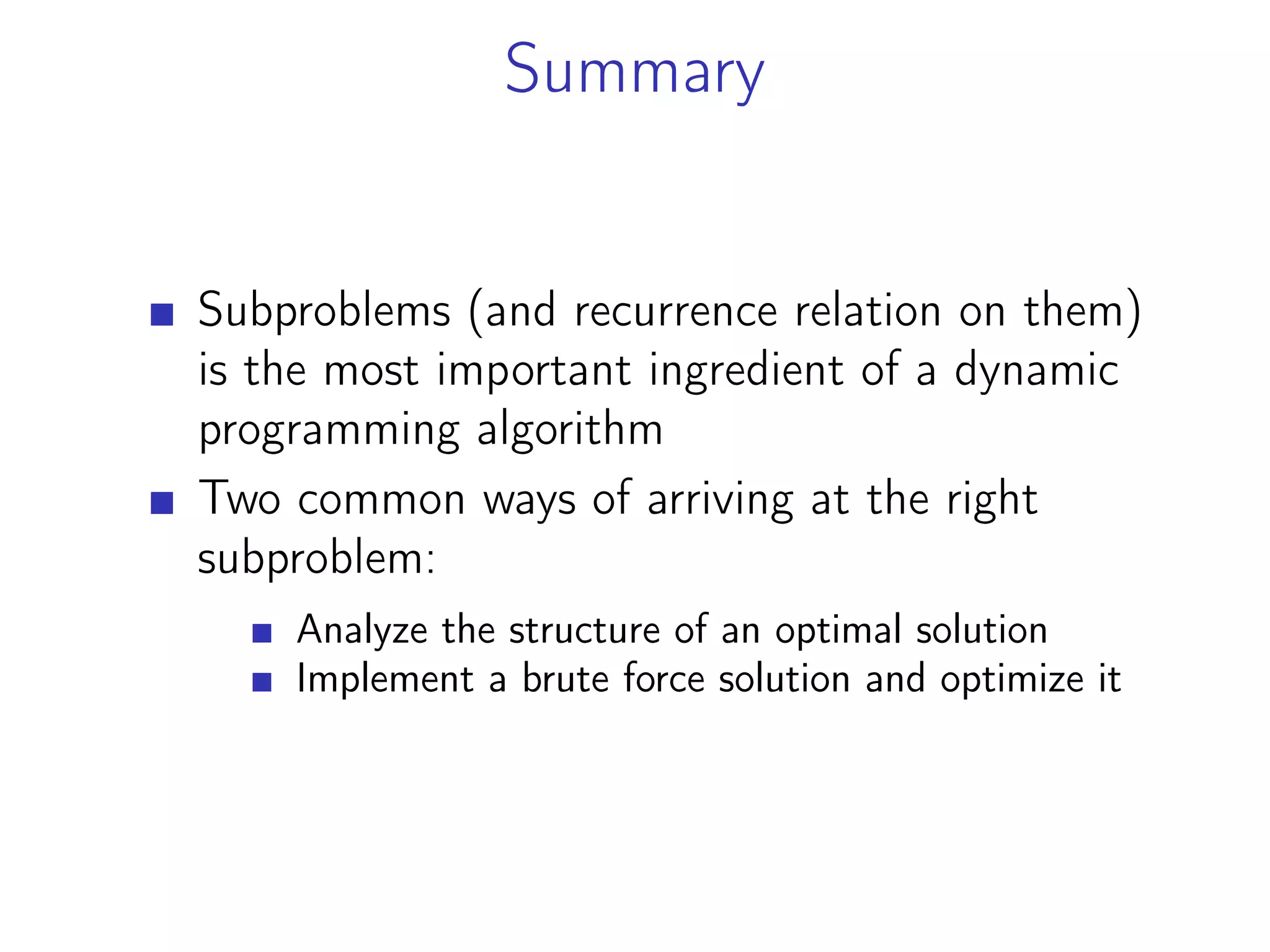
![Subproblems: Review
1 Longest increasing subsequence: LIS(i) is the
length of longest common subsequence ending
at element A[i]
2 Edit distance: ED(i, j) is the edit distance
between prefixes of length i and j
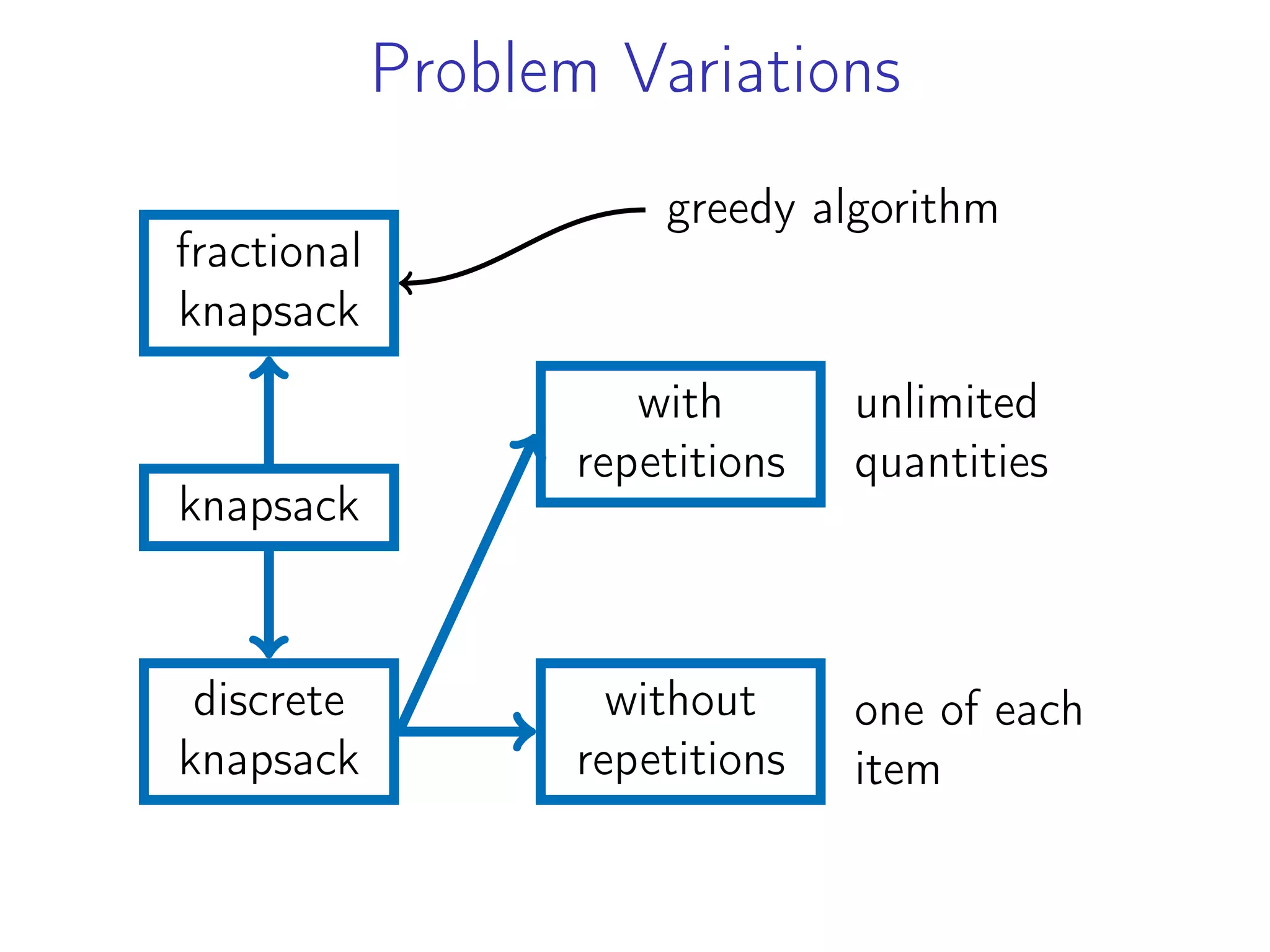
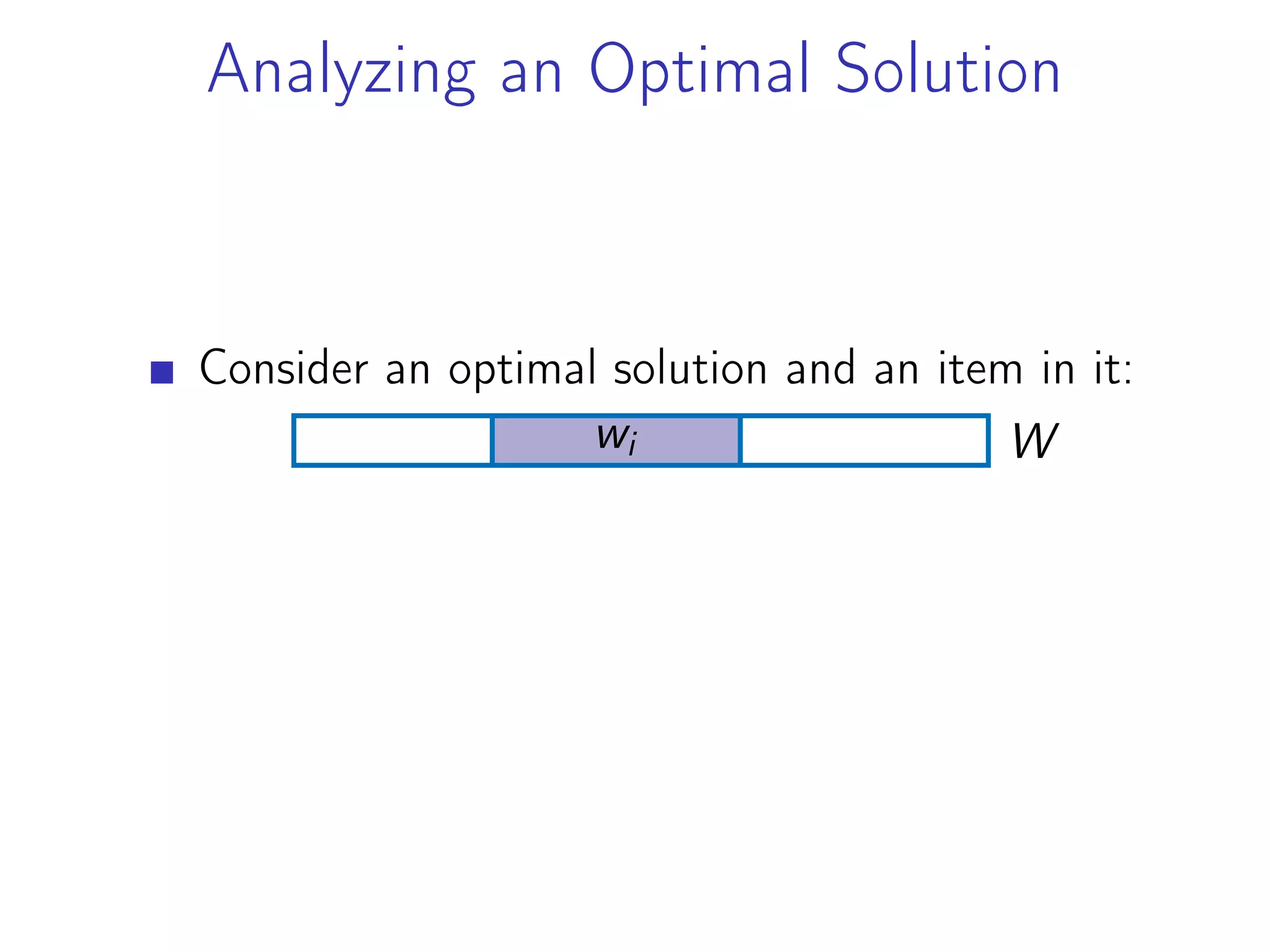
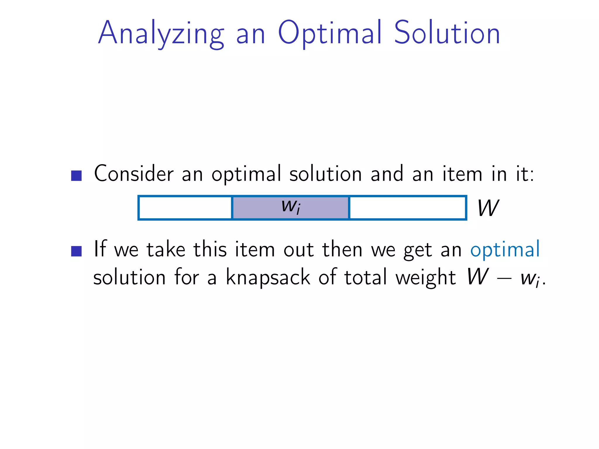
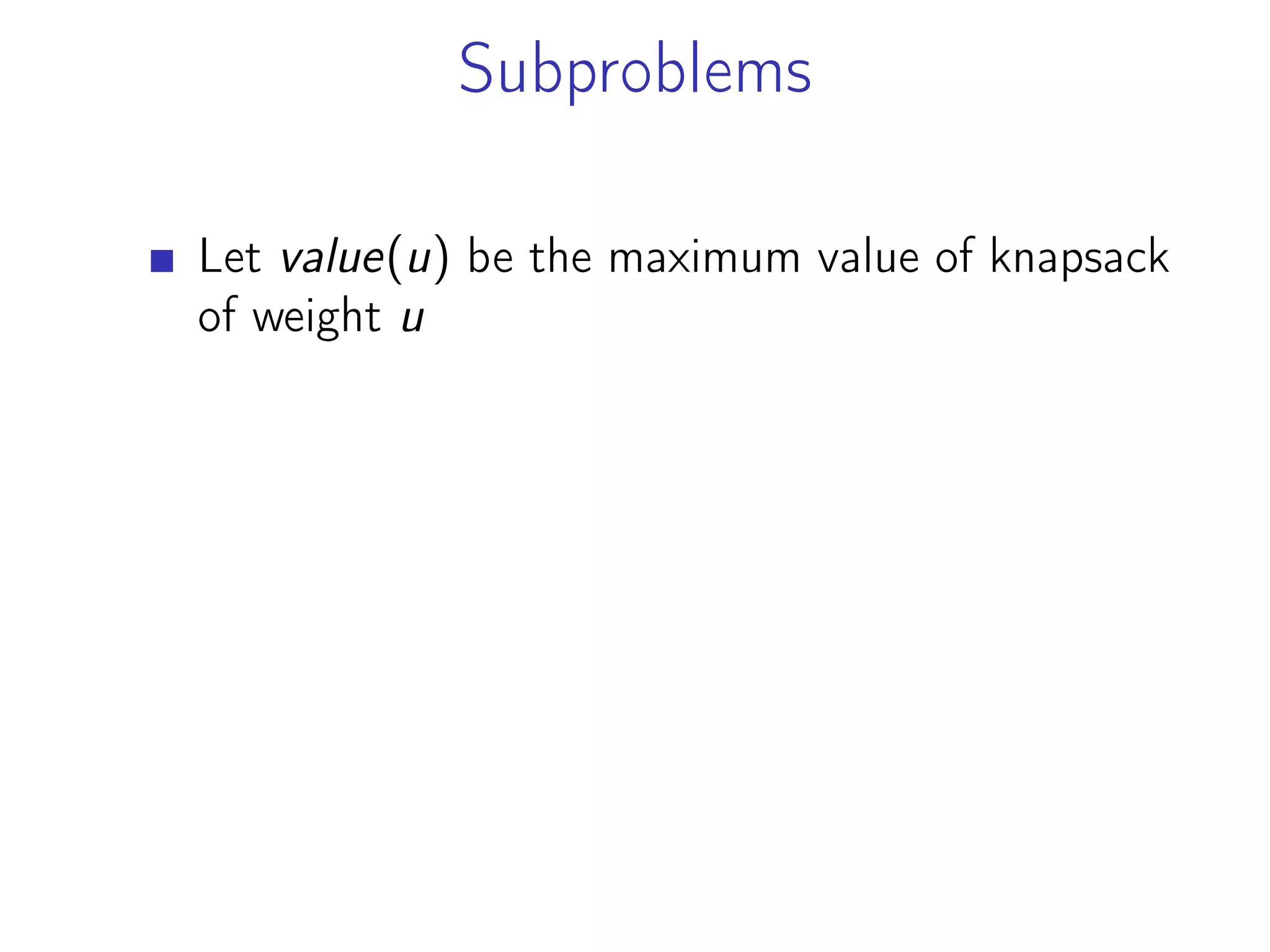
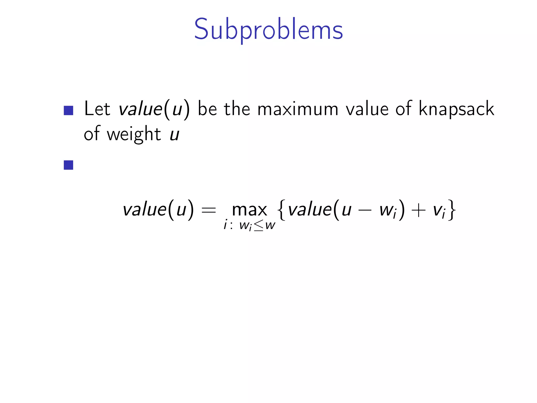
3 Knapsack: K(w) is the optimal value of
a knapsack of total weight w
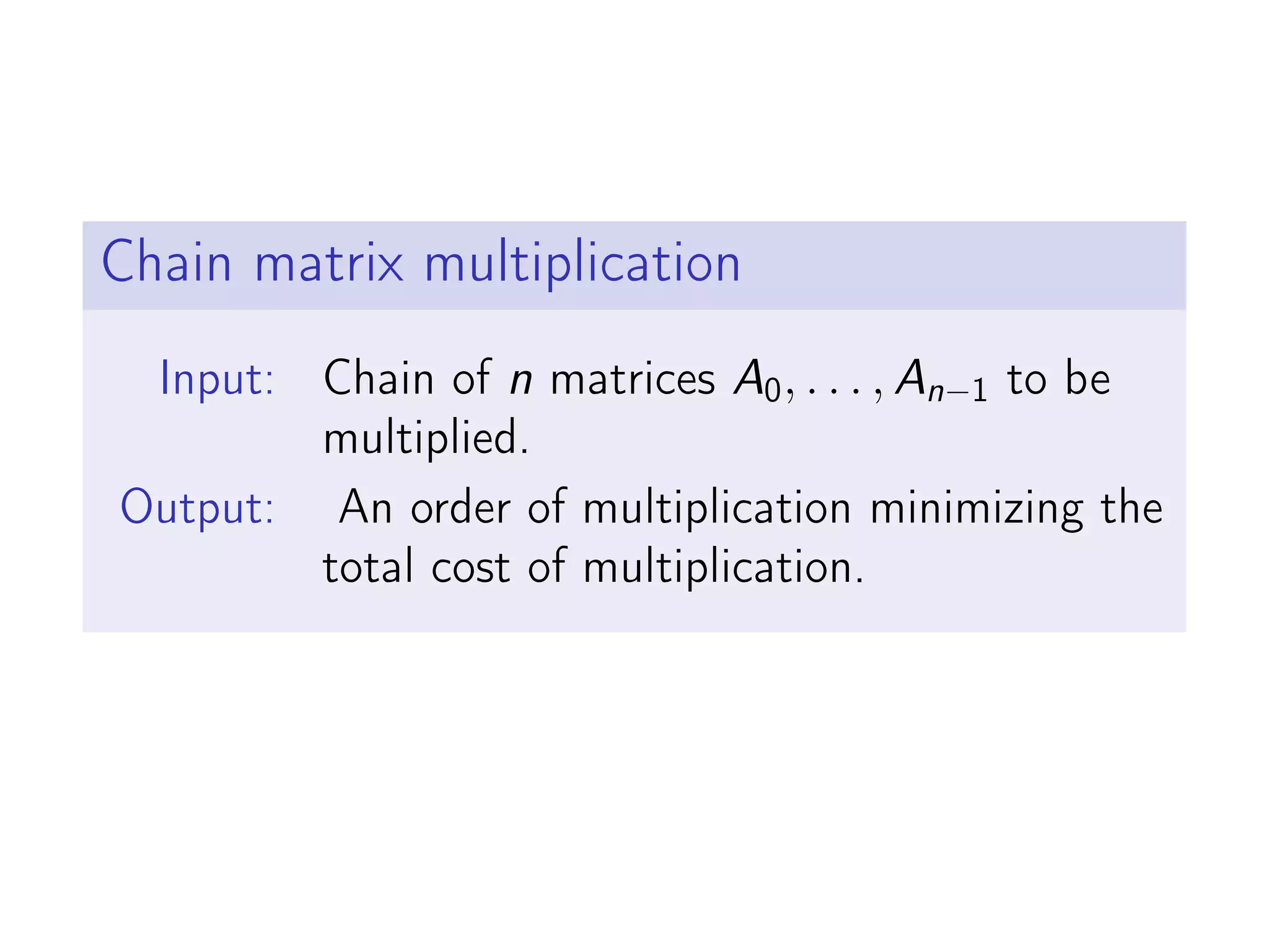
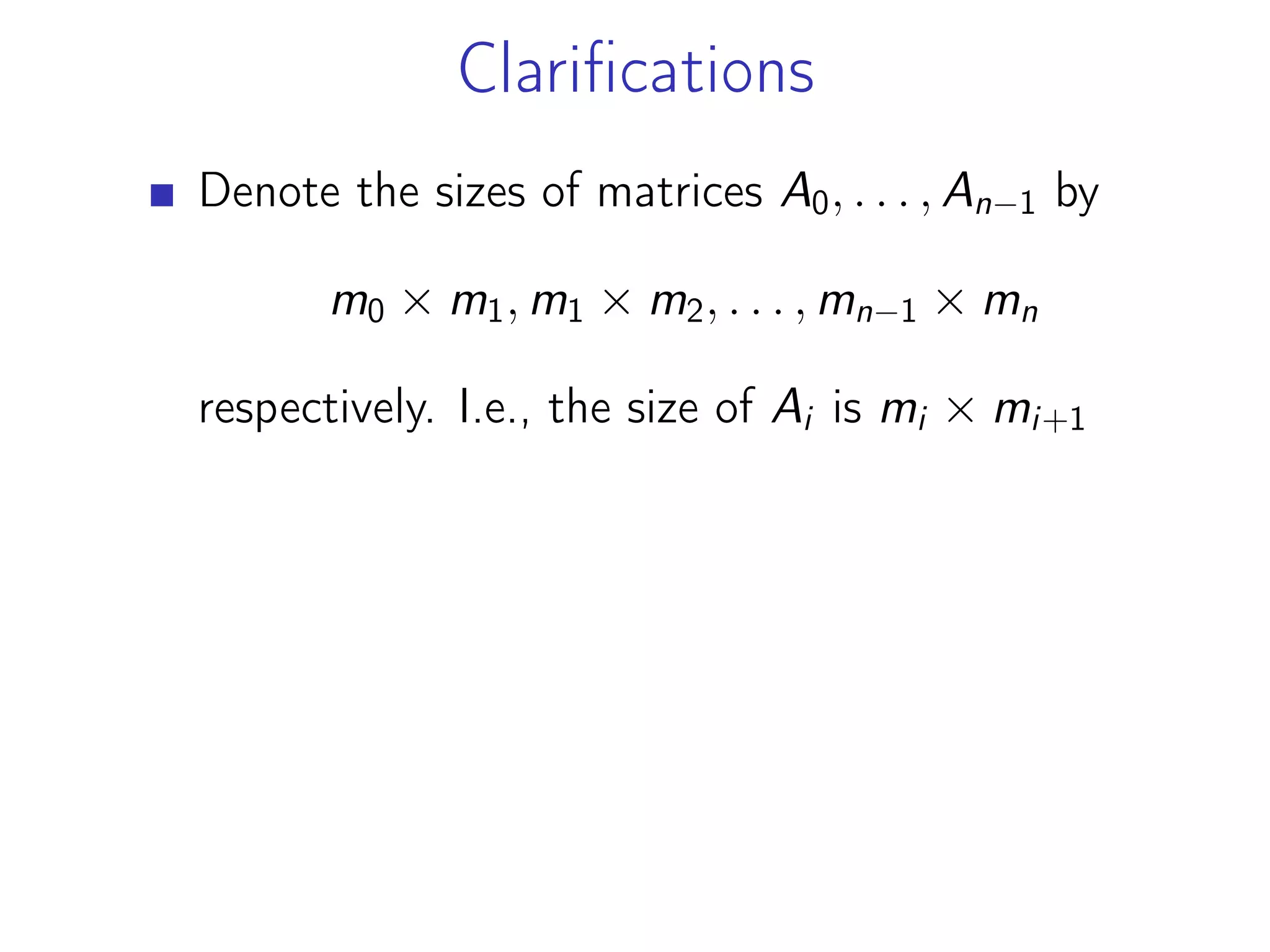
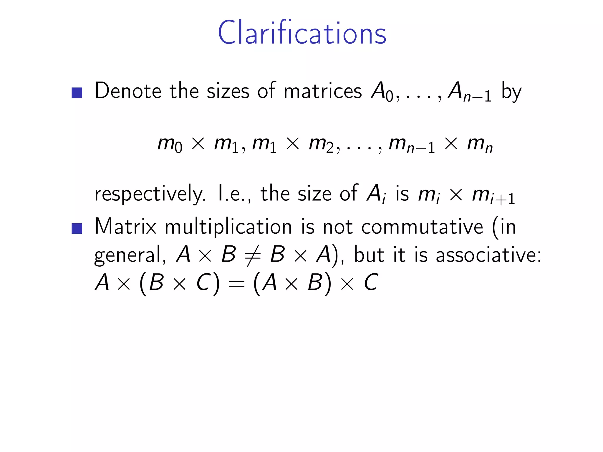
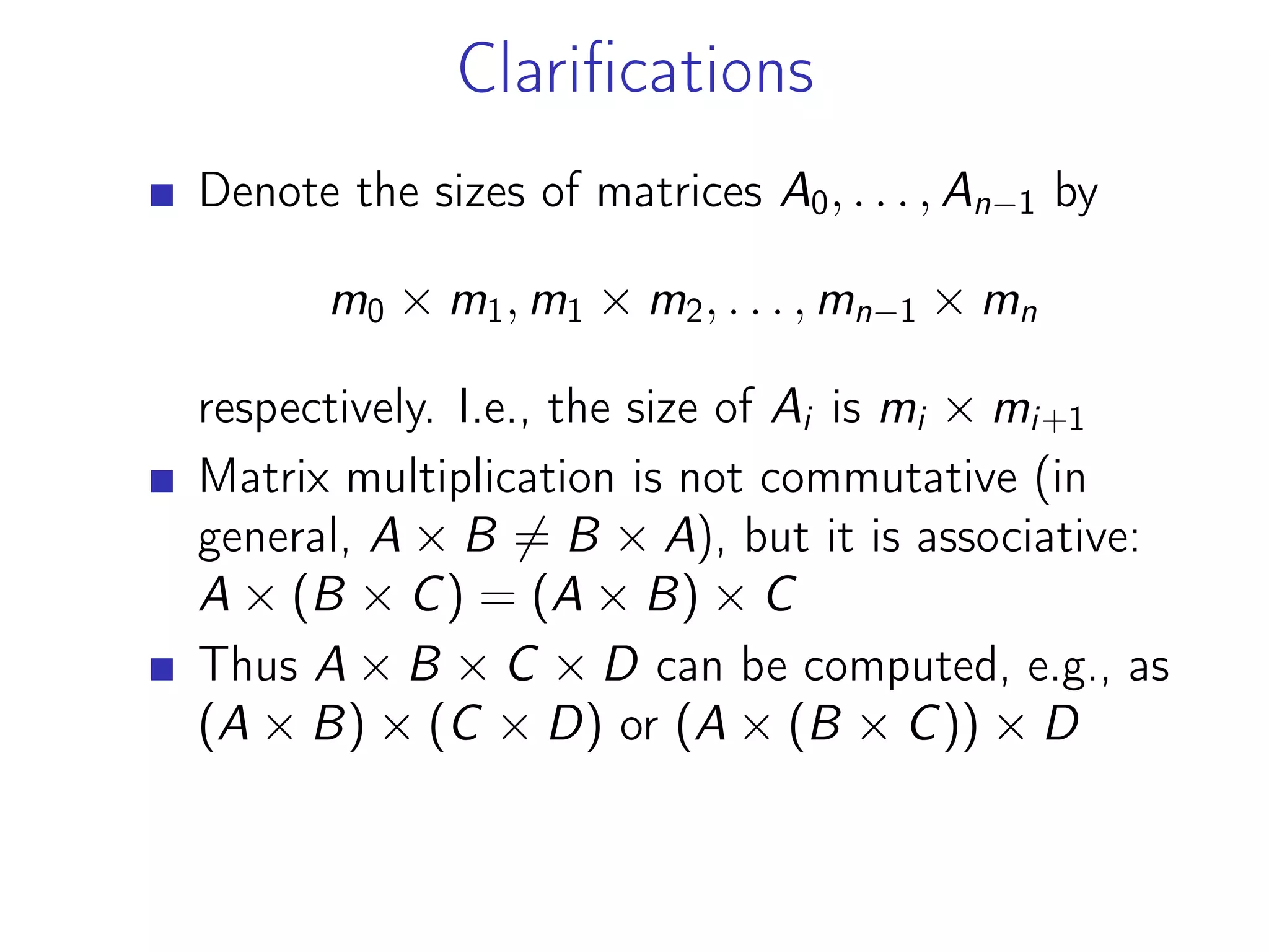
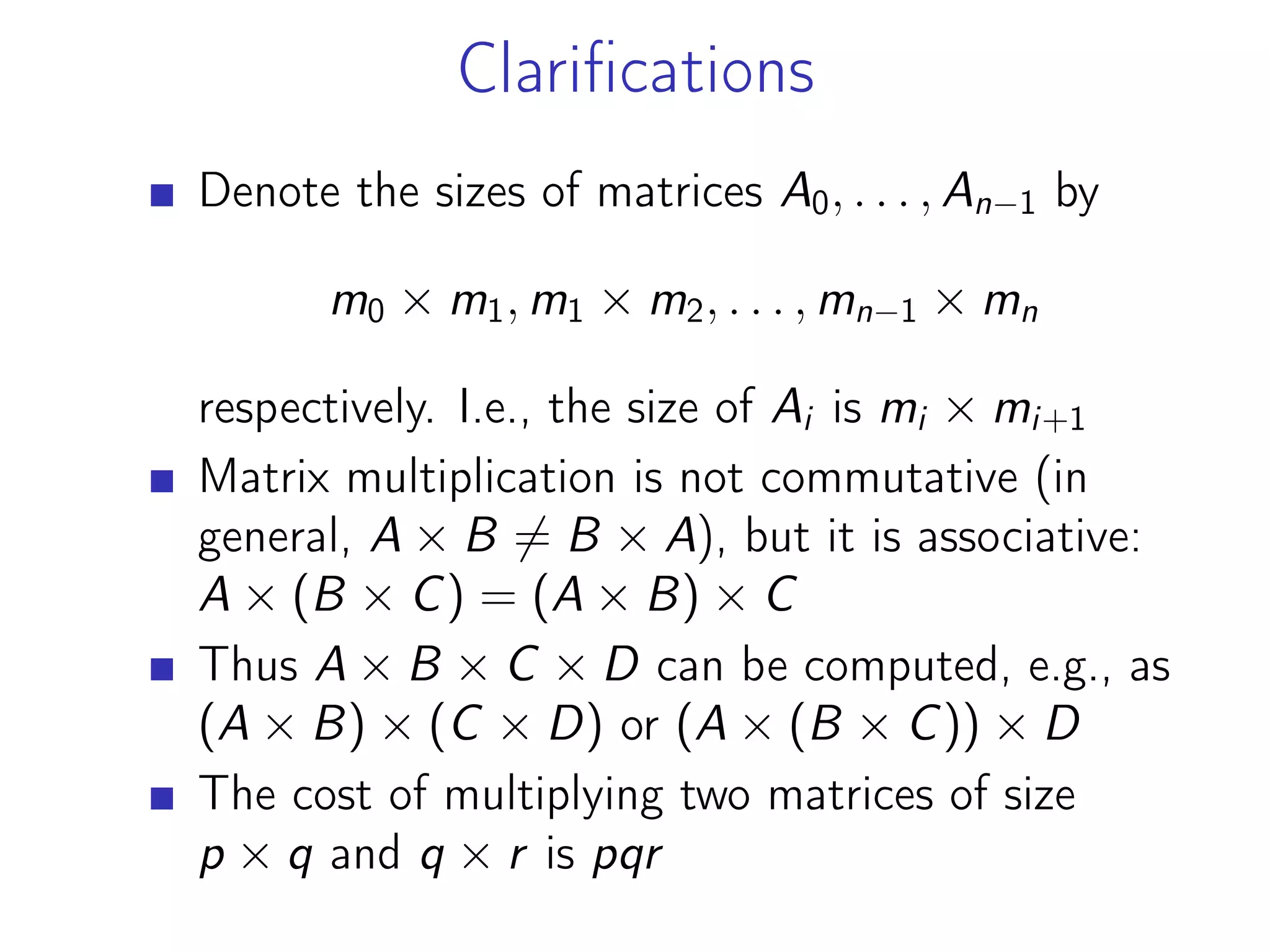
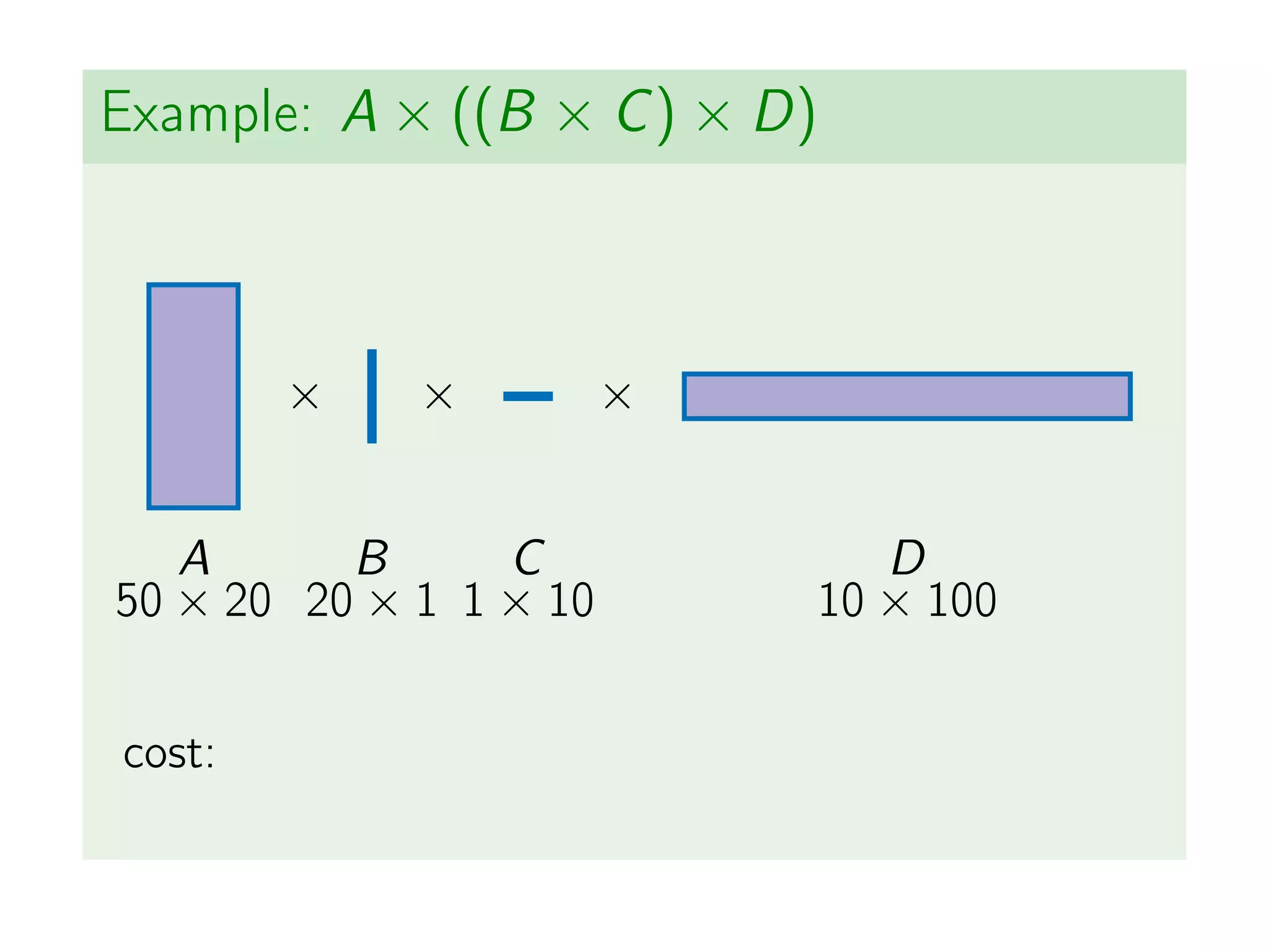
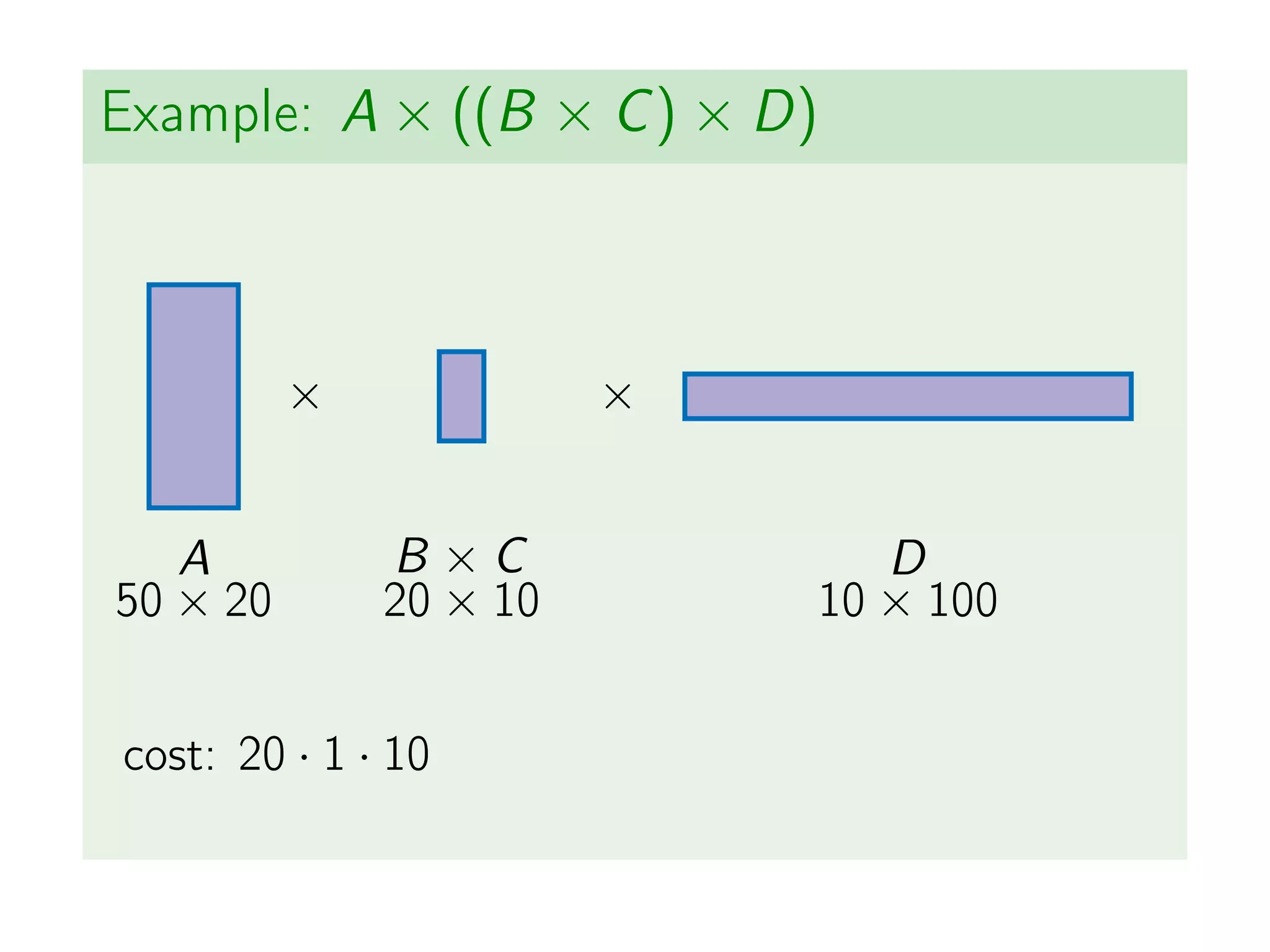
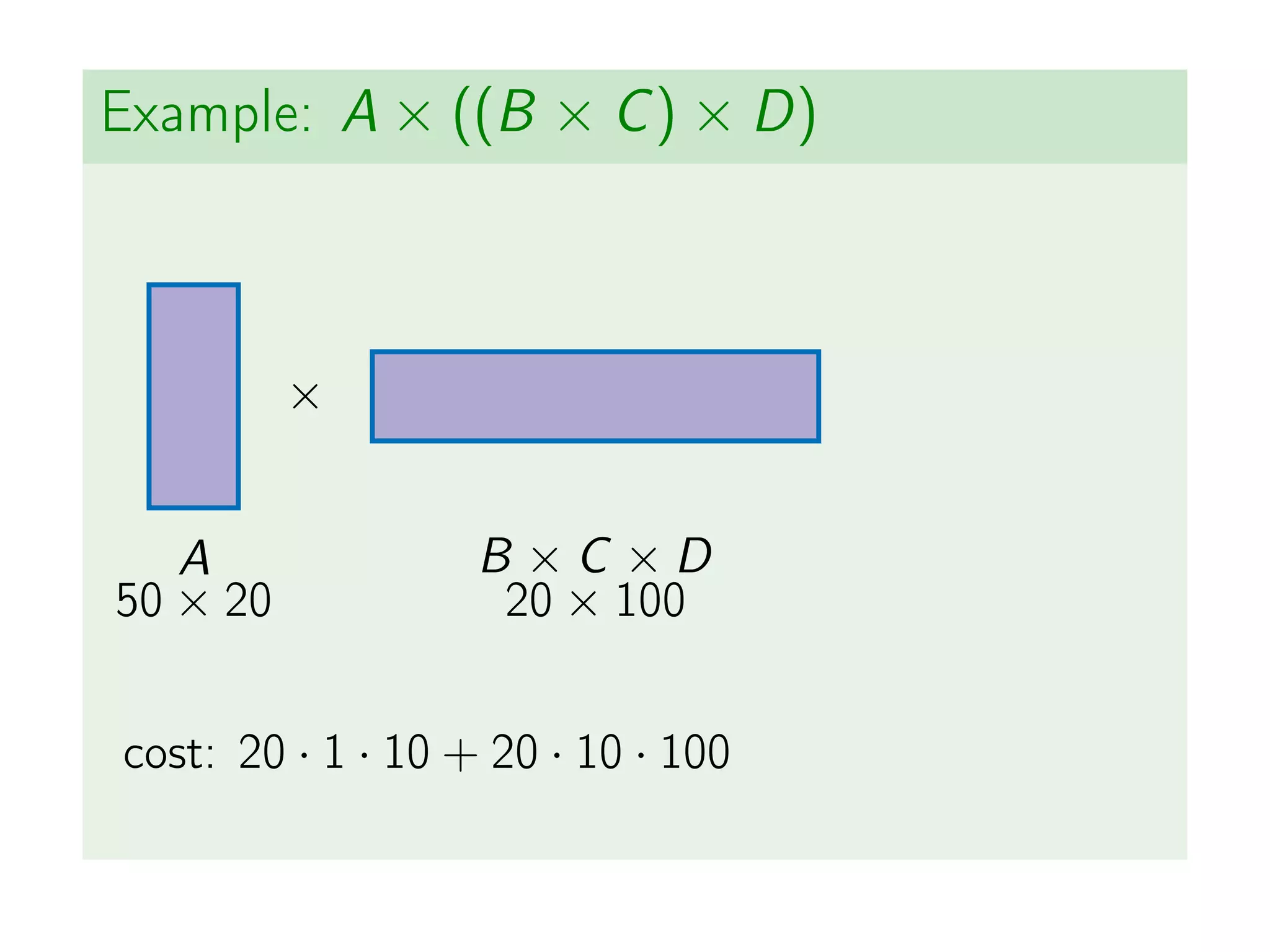
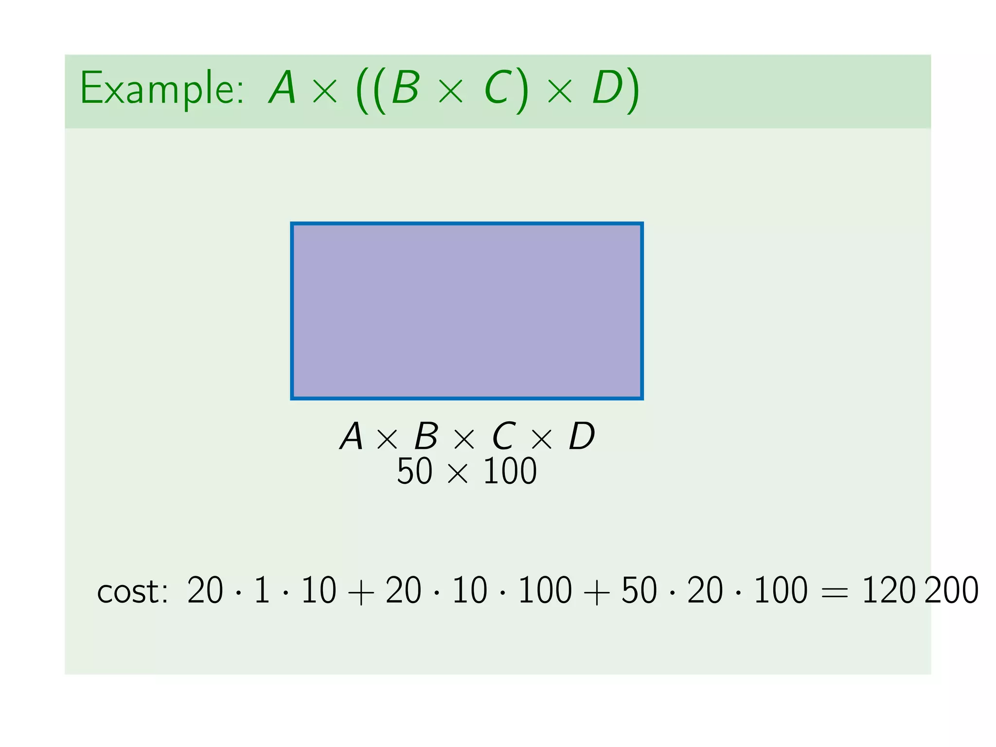
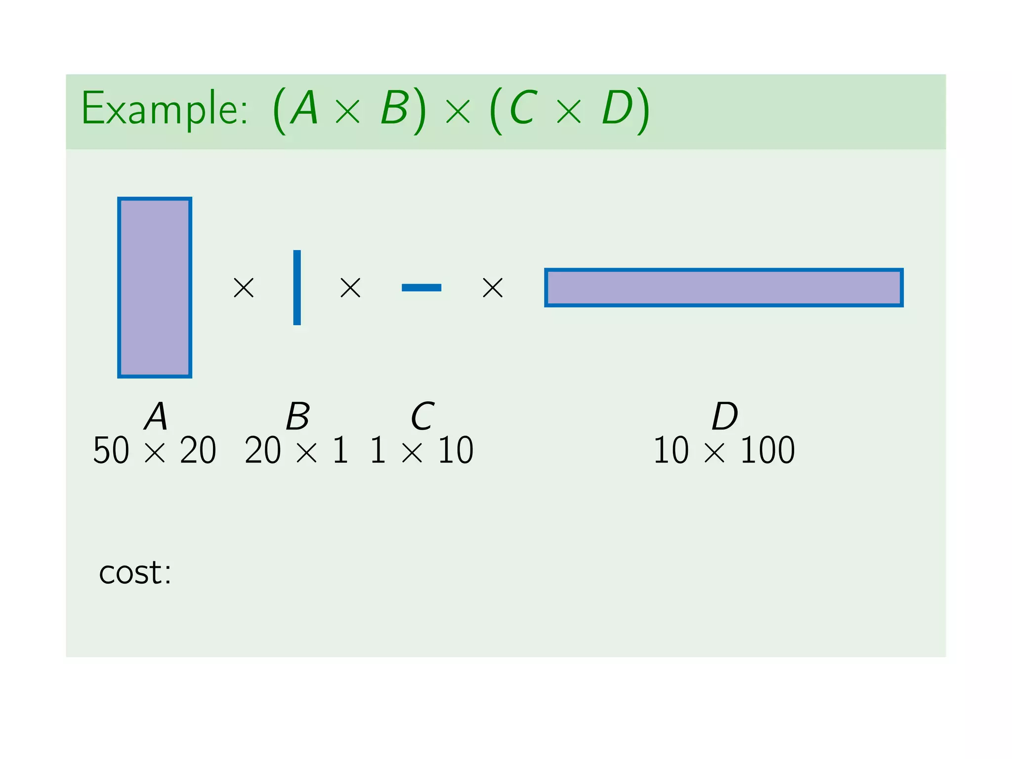
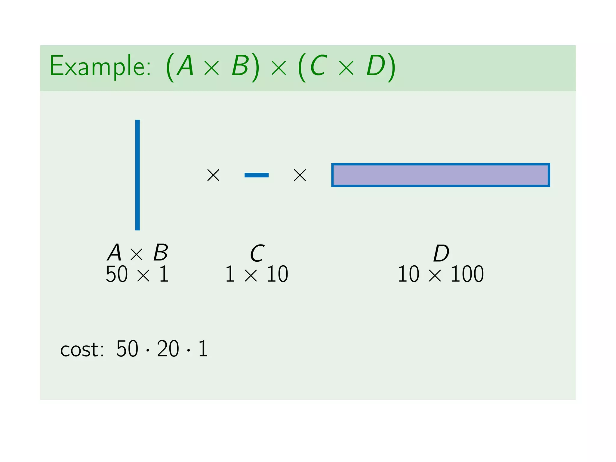
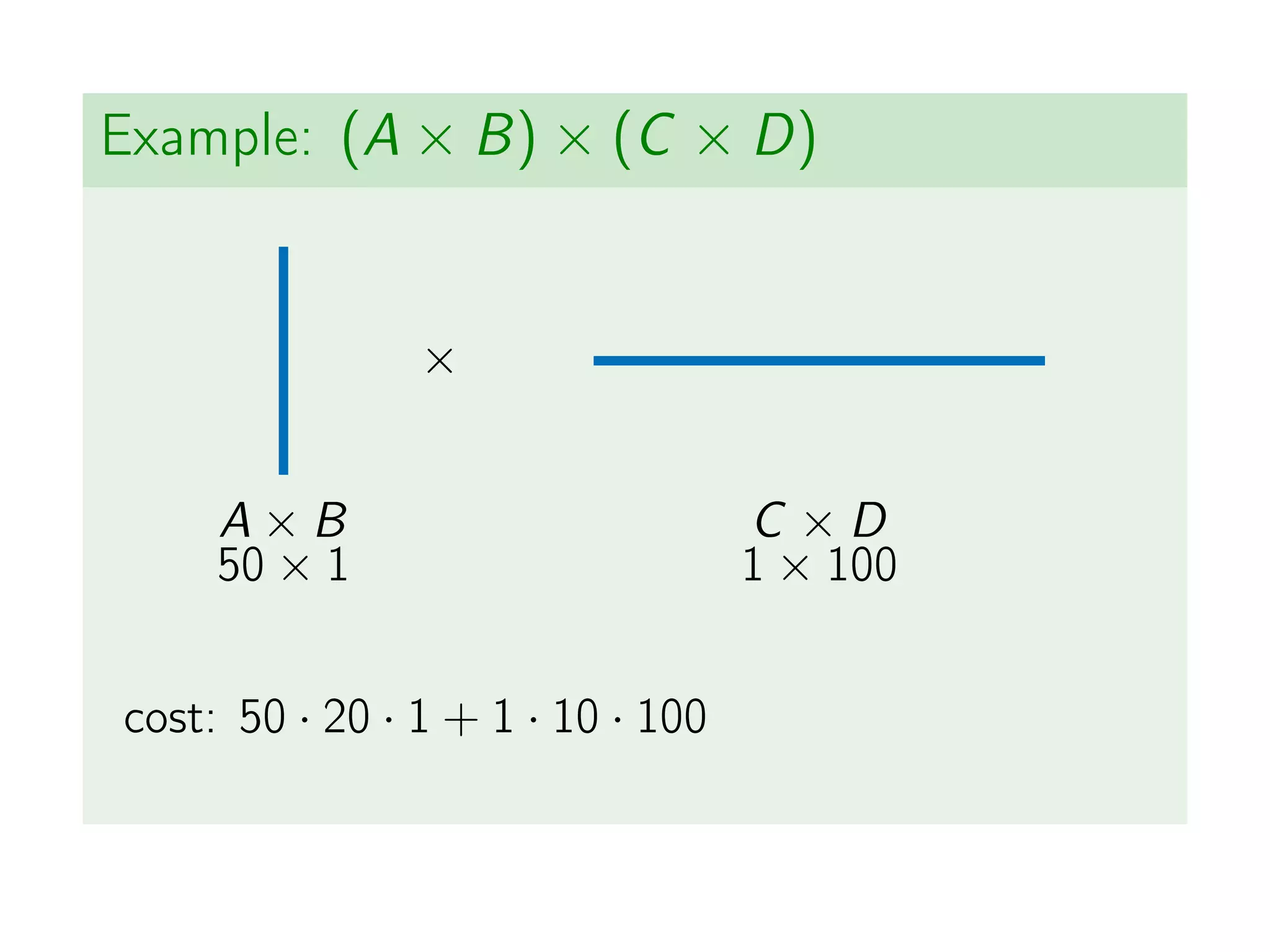
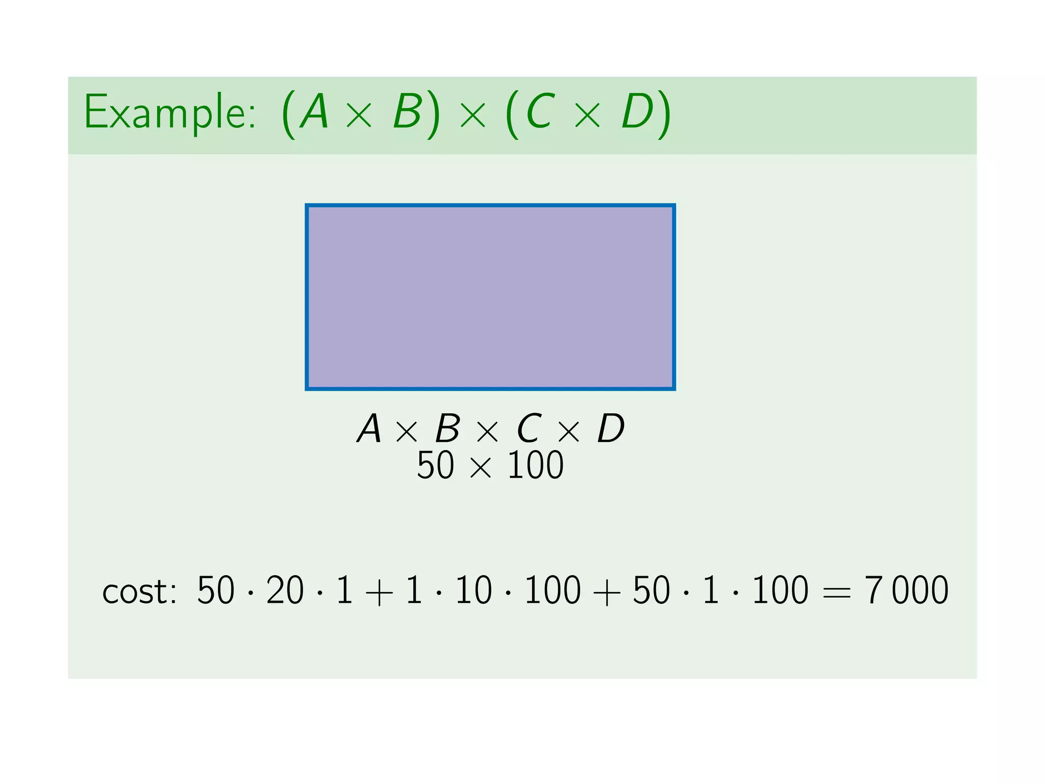
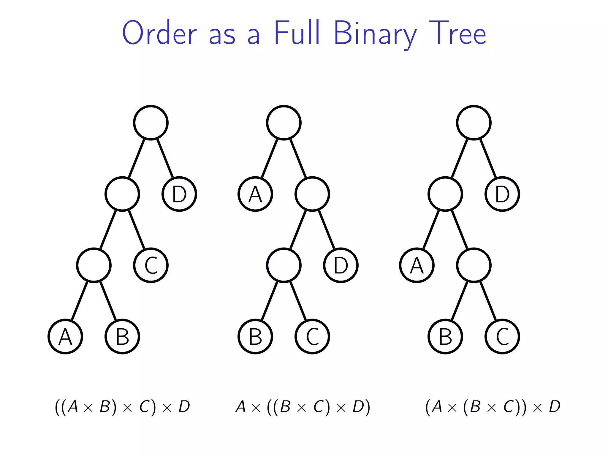
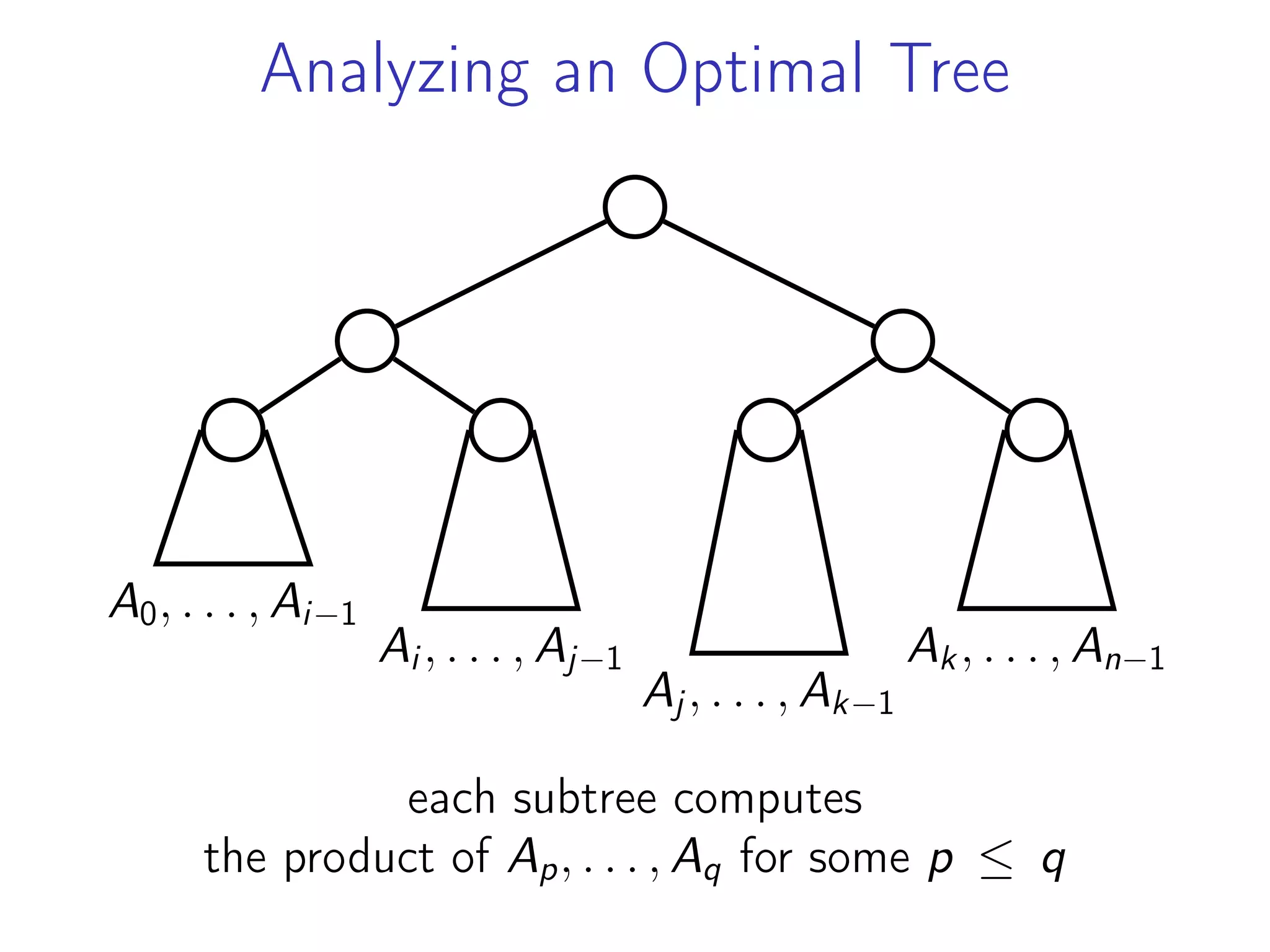
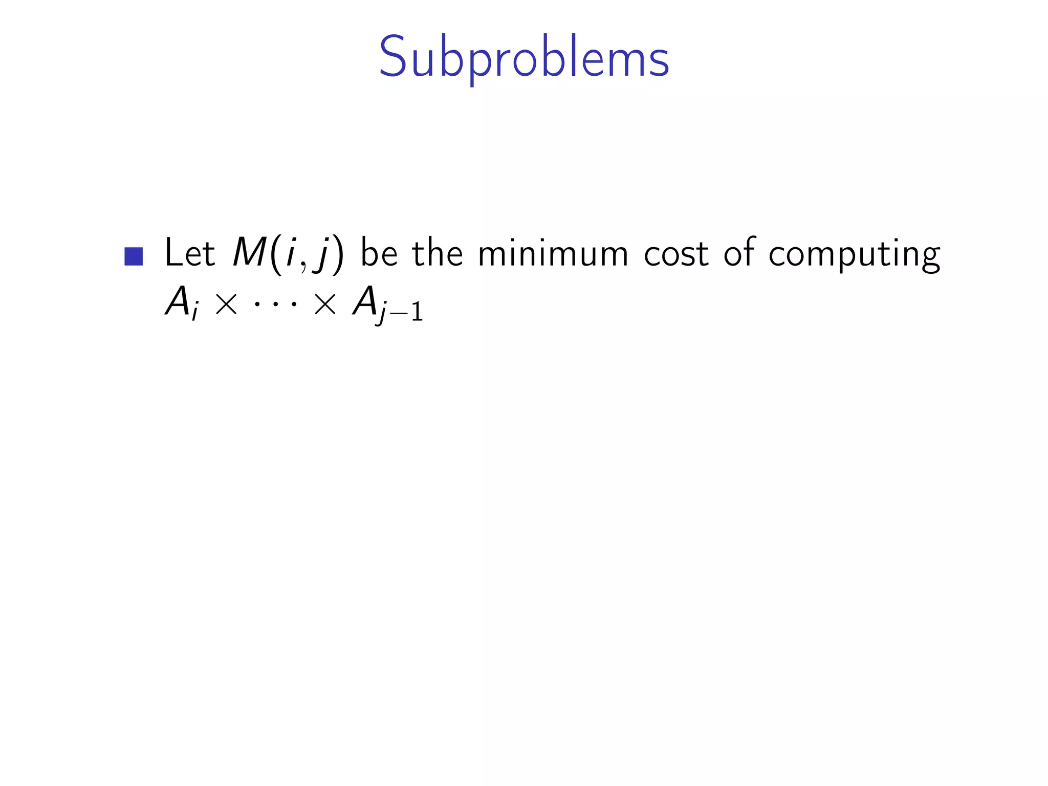
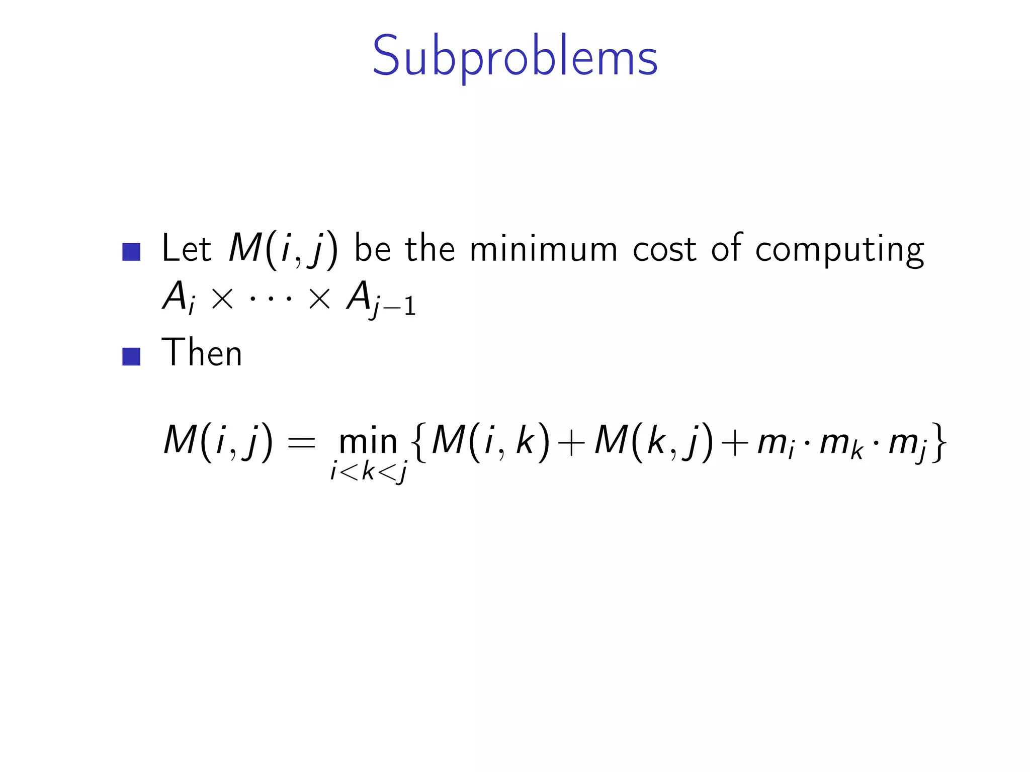
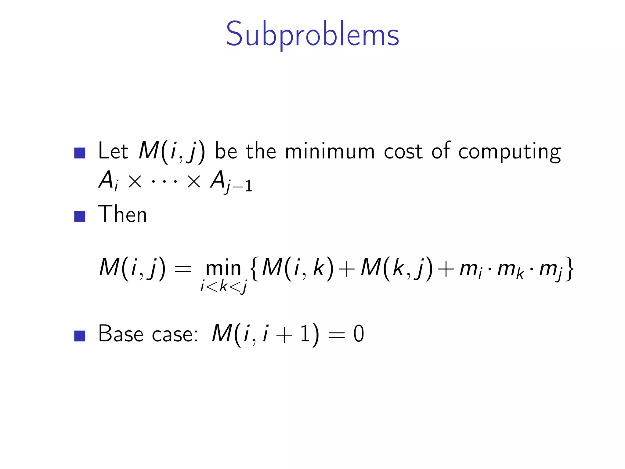
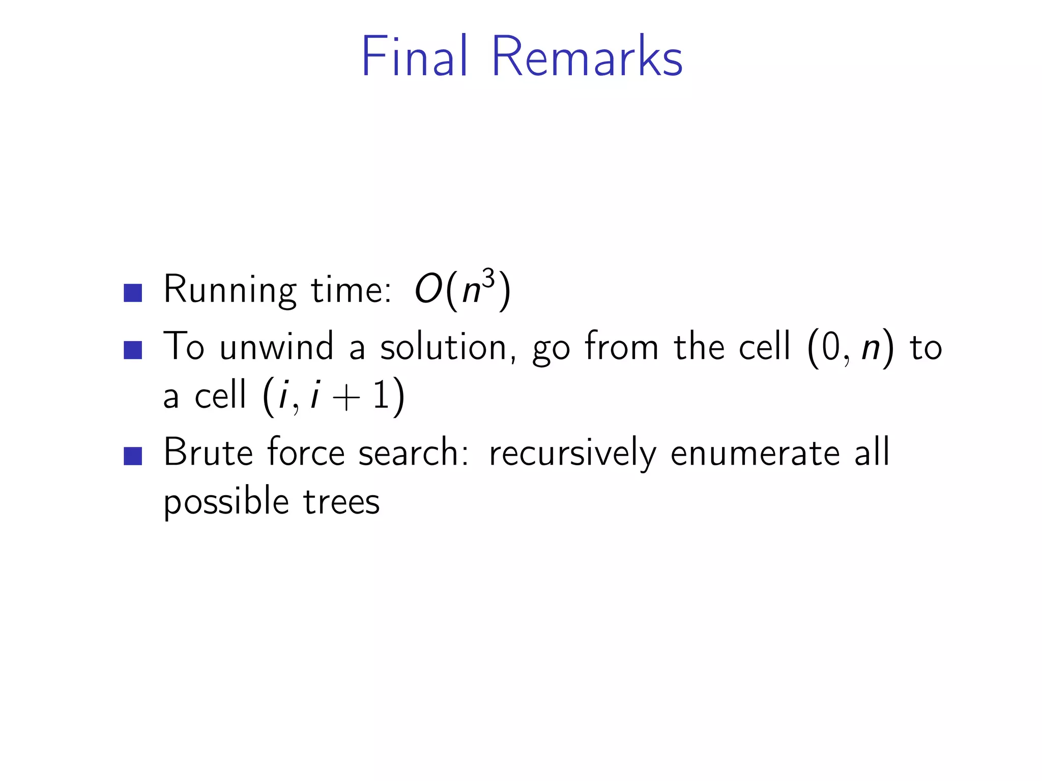
4 Chain matrix multiplication M(i, j) is the
optimal cost of multiplying matrices through i
to j − 1](https://image.slidesharecdn.com/dynamicprograming-220116082321/75/Dynamic-programing-264-2048.jpg)


![Memoization
1 def f i b (n ) :
2 i f n <= 1:
3 return n
4 return f i b (n − 1) + f i b (n − 2)
1 T = dict()
2
3 def f i b (n ) :
4 if n not in T:
5 i f n <= 1:
6 T[n] = n
7 else :
8 T[n] = f i b (n − 1) + f i b (n − 2)
9
10 return T[n]](https://crownmelresort.com/image.slidesharecdn.com/dynamicprograming-220116082321/75/Dynamic-programing-21-2048.jpg)


![Iterative Algorithm
1 def f i b (n ) :
2 T = [ None ] * (n + 1)
3 T[ 0 ] , T[ 1 ] = 0 , 1
4
5 for i in range (2 , n + 1 ) :
6 T[ i ] = T[ i − 1] + T[ i − 2]
7
8 return T[ n ]](https://crownmelresort.com/image.slidesharecdn.com/dynamicprograming-220116082321/75/Dynamic-programing-29-2048.jpg)


![Longest Increasing Subsequence
Longest increasing subsequence
Input: An array A = [a0, a1, . . . , an−1].
Output: A longest increasing subsequence (LIS),
i.e., ai1
, ai2
, . . . , aik
such that
i1 < i2 < . . . < ik, ai1
< ai2
< · · · < aik
,
and k is maximal.](https://crownmelresort.com/image.slidesharecdn.com/dynamicprograming-220116082321/75/Dynamic-programing-39-2048.jpg)


![Subproblems and Recurrence Relation
Let LIS(i) be the optimal length of a LIS ending
at A[i]](https://crownmelresort.com/image.slidesharecdn.com/dynamicprograming-220116082321/75/Dynamic-programing-47-2048.jpg)
![Subproblems and Recurrence Relation
Let LIS(i) be the optimal length of a LIS ending
at A[i]
Then
LIS(i) = 1+max{LIS(j): j < i and A[j] < A[i]}](https://crownmelresort.com/image.slidesharecdn.com/dynamicprograming-220116082321/75/Dynamic-programing-48-2048.jpg)
![Subproblems and Recurrence Relation
Let LIS(i) be the optimal length of a LIS ending
at A[i]
Then
LIS(i) = 1+max{LIS(j): j < i and A[j] < A[i]}
Convention: maximum of an empty set is equal
to zero](https://crownmelresort.com/image.slidesharecdn.com/dynamicprograming-220116082321/75/Dynamic-programing-49-2048.jpg)
![Subproblems and Recurrence Relation
Let LIS(i) be the optimal length of a LIS ending
at A[i]
Then
LIS(i) = 1+max{LIS(j): j < i and A[j] < A[i]}
Convention: maximum of an empty set is equal
to zero
Base case: LIS(0) = 1](https://crownmelresort.com/image.slidesharecdn.com/dynamicprograming-220116082321/75/Dynamic-programing-50-2048.jpg)
![Algorithm
When we have a recurrence relation at hand,
converting it to a recursive algorithm with
memoization is just a technicality
We will use a table T to store the results:
T[i] = LIS(i)](https://crownmelresort.com/image.slidesharecdn.com/dynamicprograming-220116082321/75/Dynamic-programing-51-2048.jpg)
![Algorithm
When we have a recurrence relation at hand,
converting it to a recursive algorithm with
memoization is just a technicality
We will use a table T to store the results:
T[i] = LIS(i)
Initially, T is empty. When LIS(i) is computed,
we store its value at T[i] (so that we will never
recompute LIS(i) again)](https://crownmelresort.com/image.slidesharecdn.com/dynamicprograming-220116082321/75/Dynamic-programing-52-2048.jpg)
![Algorithm
When we have a recurrence relation at hand,
converting it to a recursive algorithm with
memoization is just a technicality
We will use a table T to store the results:
T[i] = LIS(i)
Initially, T is empty. When LIS(i) is computed,
we store its value at T[i] (so that we will never
recompute LIS(i) again)
The exact data structure behind T is not that
important at this point: it could be an array or
a hash table](https://crownmelresort.com/image.slidesharecdn.com/dynamicprograming-220116082321/75/Dynamic-programing-53-2048.jpg)
![Memoization
1 T = dict ()
2
3 def l i s (A, i ) :
4 i f i not in T:
5 T[ i ] = 1
6
7 for j in range ( i ) :
8 i f A[ j ] < A[ i ] :
9 T[ i ] = max(T[ i ] , l i s (A, j ) + 1)
10
11 return T[ i ]
12
13 A = [7 , 2 , 1 , 3 , 8 , 4 , 9 , 1 , 2 , 6 , 5 , 9 , 3]
14 print (max( l i s (A, i ) for i in range ( len (A) ) ) )](https://crownmelresort.com/image.slidesharecdn.com/dynamicprograming-220116082321/75/Dynamic-programing-54-2048.jpg)


![Iterative Algorithm
1 def l i s (A) :
2 T = [ None ] * len (A)
3
4 for i in range ( len (A ) ) :
5 T[ i ] = 1
6 for j in range ( i ) :
7 i f A[ j ] < A[ i ] and T[ i ] < T[ j ] + 1:
8 T[ i ] = T[ j ] + 1
9
10 return max(T[ i ] for i in range ( len (A) ) )](https://crownmelresort.com/image.slidesharecdn.com/dynamicprograming-220116082321/75/Dynamic-programing-59-2048.jpg)
![Iterative Algorithm
1 def l i s (A) :
2 T = [ None ] * len (A)
3
4 for i in range ( len (A ) ) :
5 T[ i ] = 1
6 for j in range ( i ) :
7 i f A[ j ] < A[ i ] and T[ i ] < T[ j ] + 1:
8 T[ i ] = T[ j ] + 1
9
10 return max(T[ i ] for i in range ( len (A) ) )
Crucial property: when computing T[i], T[j] for
all j < i have already been computed](https://crownmelresort.com/image.slidesharecdn.com/dynamicprograming-220116082321/75/Dynamic-programing-60-2048.jpg)
![Iterative Algorithm
1 def l i s (A) :
2 T = [ None ] * len (A)
3
4 for i in range ( len (A ) ) :
5 T[ i ] = 1
6 for j in range ( i ) :
7 i f A[ j ] < A[ i ] and T[ i ] < T[ j ] + 1:
8 T[ i ] = T[ j ] + 1
9
10 return max(T[ i ] for i in range ( len (A) ) )
Crucial property: when computing T[i], T[j] for
all j < i have already been computed
Running time: O(n2
)](https://crownmelresort.com/image.slidesharecdn.com/dynamicprograming-220116082321/75/Dynamic-programing-61-2048.jpg)


![Adjusting the Algorithm
1 def l i s (A) :
2 T = [ None ] * len (A)
3 prev = [None] * len(A)
4
5 for i in range ( len (A ) ) :
6 T[ i ] = 1
7 prev[i] = -1
8 for j in range ( i ) :
9 i f A[ j ] < A[ i ] and T[ i ] < T[ j ] + 1:
10 T[ i ] = T[ j ] + 1
11 prev[i] = j](https://crownmelresort.com/image.slidesharecdn.com/dynamicprograming-220116082321/75/Dynamic-programing-65-2048.jpg)


![Unwinding Solution
1 l a s t = 0
2 for i in range (1 , len (A ) ) :
3 i f T[ i ] > T[ l a s t ] :
4 l a s t = i
5
6 l i s= [ ]
7 c u r r e n t = l a s t
8 while c u r r e n t >= 0:
9 l i s . append ( c u r r e n t )
10 c u r r e n t = prev [ c u r r e n t ]
11 l i s . r e v e r s e ()
12 return [A[ i ] for i in l i s ]](https://crownmelresort.com/image.slidesharecdn.com/dynamicprograming-220116082321/75/Dynamic-programing-77-2048.jpg)


![Brute Force: Code
1 def l i s (A, seq ) :
2 r e s u l t = len ( seq )
3
4 i f len ( seq ) == 0:
5 last_index = −1
6 last_element = float ( "−i n f " )
7 else :
8 last_index = seq [ −1]
9 last_element = A[ last_index ]
10
11 for i in range ( last_index + 1 , len (A ) ) :
12 i f A[ i ] > last_element :
13 r e s u l t = max( r e s u l t , l i s (A, seq + [ i ] ) )
14
15 return r e s u l t
16
17 print ( l i s (A=[7 , 2 , 1 , 3 , 8 , 4 , 9] , seq =[]))](https://crownmelresort.com/image.slidesharecdn.com/dynamicprograming-220116082321/75/Dynamic-programing-98-2048.jpg)


![Optimized Code
1 def l i s (A, seq_len , last_index ) :
2 i f last_index == −1:
3 last_element = float ( "−i n f " )
4 else :
5 last_element = A[ last_index ]
6
7 r e s u l t = seq_len
8
9 for i in range ( last_index + 1 , len (A ) ) :
10 i f A[ i ] > last_element :
11 r e s u l t = max( r e s u l t ,
12 l i s (A, seq_len + 1 , i ))
13
14 return r e s u l t
15
16 print ( l i s ( [ 3 , 2 , 7 , 8 , 9 , 5 , 8] , 0 , −1))](https://crownmelresort.com/image.slidesharecdn.com/dynamicprograming-220116082321/75/Dynamic-programing-103-2048.jpg)


![Resulting Code
1 def l i s (A, last_index ) :
2 i f last_index == −1:
3 last_element = float ( "−i n f " )
4 else :
5 last_element = A[ last_index ]
6
7 r e s u l t = 0
8
9 for i in range ( last_index + 1 , len (A ) ) :
10 i f A[ i ] > last_element :
11 r e s u l t = max( r e s u l t , 1 + l i s (A, i ))
12
13 return r e s u l t
14
15 print ( l i s ( [ 8 , 2 , 3 , 4 , 5 , 6 , 7] , −1))](https://crownmelresort.com/image.slidesharecdn.com/dynamicprograming-220116082321/75/Dynamic-programing-108-2048.jpg)
![Resulting Code
1 def l i s (A, last_index ) :
2 i f last_index == −1:
3 last_element = float ( "−i n f " )
4 else :
5 last_element = A[ last_index ]
6
7 r e s u l t = 0
8
9 for i in range ( last_index + 1 , len (A ) ) :
10 i f A[ i ] > last_element :
11 r e s u l t = max( r e s u l t , 1 + l i s (A, i ))
12
13 return r e s u l t
14
15 print ( l i s ( [ 8 , 2 , 3 , 4 , 5 , 6 , 7] , −1))
It remains to add memoization!](https://crownmelresort.com/image.slidesharecdn.com/dynamicprograming-220116082321/75/Dynamic-programing-109-2048.jpg)


![Statement
Edit distance
Input: Two strings A[0 . . . n − 1] and
B[0 . . . m − 1].
Output: The minimal number of insertions,
deletions, and substitutions needed to
transform A to B. This number is known
as edit distance or Levenshtein distance.](https://crownmelresort.com/image.slidesharecdn.com/dynamicprograming-220116082321/75/Dynamic-programing-115-2048.jpg)


![Analyzing an Optimal Alignment
A[0 . . . n − 1]
B[0 . . . m − 1]](https://crownmelresort.com/image.slidesharecdn.com/dynamicprograming-220116082321/75/Dynamic-programing-124-2048.jpg)
![Analyzing an Optimal Alignment
A[0 . . . n − 1]
B[0 . . . m − 1]
A[0 . . . n − 1] −
B[0 . . . m − 2] B[m − 1]
insertion](https://crownmelresort.com/image.slidesharecdn.com/dynamicprograming-220116082321/75/Dynamic-programing-125-2048.jpg)
![Analyzing an Optimal Alignment
A[0 . . . n − 1]
B[0 . . . m − 1]
A[0 . . . n − 1] −
B[0 . . . m − 2] B[m − 1]
insertion
A[0 . . . n − 2] A[n − 1]
B[0 . . . m − 1] −
deletion](https://crownmelresort.com/image.slidesharecdn.com/dynamicprograming-220116082321/75/Dynamic-programing-126-2048.jpg)
![Analyzing an Optimal Alignment
A[0 . . . n − 1]
B[0 . . . m − 1]
A[0 . . . n − 1] −
B[0 . . . m − 2] B[m − 1]
insertion
A[0 . . . n − 2] A[n − 1]
B[0 . . . m − 1] −
deletion
A[0 . . . n − 2] A[n − 1]
B[0 . . . m − 2] B[m − 1]
match/mismatch](https://crownmelresort.com/image.slidesharecdn.com/dynamicprograming-220116082321/75/Dynamic-programing-127-2048.jpg)
![Subproblems
Let ED(i, j) be the edit distance of
A[0 . . . i − 1] and B[0 . . . j − 1].](https://crownmelresort.com/image.slidesharecdn.com/dynamicprograming-220116082321/75/Dynamic-programing-128-2048.jpg)
![Subproblems
Let ED(i, j) be the edit distance of
A[0 . . . i − 1] and B[0 . . . j − 1].
We know for sure that the last column of an
optimal alignment is either an insertion, a
deletion, or a match/mismatch.](https://crownmelresort.com/image.slidesharecdn.com/dynamicprograming-220116082321/75/Dynamic-programing-129-2048.jpg)
![Subproblems
Let ED(i, j) be the edit distance of
A[0 . . . i − 1] and B[0 . . . j − 1].
We know for sure that the last column of an
optimal alignment is either an insertion, a
deletion, or a match/mismatch.
What is left is an optimal alignment of the
corresponding two prefixes (by cut-and-paste).](https://crownmelresort.com/image.slidesharecdn.com/dynamicprograming-220116082321/75/Dynamic-programing-130-2048.jpg)
![Recurrence Relation
ED(i, j) = min
⎧
⎪
⎨
⎪
⎩
ED(i, j − 1) + 1
ED(i − 1, j) + 1
ED(i − 1, j − 1) + diff(A[i], B[j])](https://crownmelresort.com/image.slidesharecdn.com/dynamicprograming-220116082321/75/Dynamic-programing-131-2048.jpg)
![Recurrence Relation
ED(i, j) = min
⎧
⎪
⎨
⎪
⎩
ED(i, j − 1) + 1
ED(i − 1, j) + 1
ED(i − 1, j − 1) + diff(A[i], B[j])
Base case: ED(i, 0) = i, ED(0, j) = j](https://crownmelresort.com/image.slidesharecdn.com/dynamicprograming-220116082321/75/Dynamic-programing-132-2048.jpg)
![Recursive Algorithm
1 T = dict ()
2
3 def edit_distance (a , b , i , j ) :
4 i f not ( i , j ) in T:
5 i f i == 0: T[ i , j ] = j
6 e l i f j == 0: T[ i , j ] = i
7 else :
8 d i f f = 0 i f a [ i − 1] == b [ j − 1] else 1
9 T[ i , j ] = min(
10 edit_distance (a , b , i − 1 , j ) + 1 ,
11 edit_distance (a , b , i , j − 1) + 1 ,
12 edit_distance (a , b , i − 1 , j − 1) + d i f f )
13
14 return T[ i , j ]
15
16
17 print ( edit_distance ( a=" e d i t i n g " , b=" d i s t a n c e " ,
18 i =7, j =8))](https://crownmelresort.com/image.slidesharecdn.com/dynamicprograming-220116082321/75/Dynamic-programing-133-2048.jpg)


![Iterative Algorithm
1 def edit_distance (a , b ) :
2 T = [ [ f l o a t ( " i n f " ) ] * ( len (b) + 1)
3 for _ in range ( len ( a ) + 1 ) ]
4 for i in range ( len ( a ) + 1 ) :
5 T[ i ] [ 0 ] = i
6 for j in range ( len (b) + 1 ) :
7 T [ 0 ] [ j ] = j
8
9 for i in range (1 , len ( a ) + 1 ) :
10 for j in range (1 , len (b) + 1 ) :
11 d i f f = 0 i f a [ i − 1] == b [ j − 1] else 1
12 T[ i ] [ j ] = min(T[ i − 1 ] [ j ] + 1 ,
13 T[ i ] [ j − 1] + 1 ,
14 T[ i − 1 ] [ j − 1] + d i f f )
15
16 return T[ len ( a ) ] [ len (b ) ]
17
18
19 print ( edit_distance ( a=" d i s t a n c e " , b=" e d i t i n g " ))](https://crownmelresort.com/image.slidesharecdn.com/dynamicprograming-220116082321/75/Dynamic-programing-137-2048.jpg)


![Reconstructing a Solution
To reconstruct a solution, we go back from the
cell (n, m) to the cell (0, 0)
If ED(i, j) = ED(i − 1, j) + 1, then there exists
an optimal alignment whose last column is a
deletion
If ED(i, j) = ED(i, j − 1) + 1, then there exists
an optimal alignment whose last column is an
insertion
If ED(i, j) = ED(i − 1, j − 1) + diff(A[i], B[j]),
then match (if A[i] = B[j]) or mismatch (if
A[i] ̸= B[j])](https://crownmelresort.com/image.slidesharecdn.com/dynamicprograming-220116082321/75/Dynamic-programing-152-2048.jpg)


![Saving Space
When filling in the matrix it is enough to keep
only the current column and the previous
column:
0
n
i
0 m
j
0
n
i
0 m
j
Thus, one can compute the edit distance of two
given strings A[1 . . . n] and B[1 . . . m] in time
O(nm) and space O(min{n, m}).](https://crownmelresort.com/image.slidesharecdn.com/dynamicprograming-220116082321/75/Dynamic-programing-165-2048.jpg)


![Generalized Recurrence Relation
min
⎧
⎪
⎨
⎪
⎩
ED(i, j − 1) + inscost(B[j]),
ED(i − 1, j) + delcost(A[i]),
ED(i − 1, j − 1) + substcost(A[i], B[j])](https://crownmelresort.com/image.slidesharecdn.com/dynamicprograming-220116082321/75/Dynamic-programing-169-2048.jpg)


![Recursive Algorithm
1 T = dict ()
2
3 def knapsack (w, v , u ) :
4 i f u not in T:
5 T[ u ] = 0
6
7 for i in range ( len (w) ) :
8 i f w[ i ] <= u :
9 T[ u ] = max(T[ u ] ,
10 knapsack (w, v , u − w[ i ] ) + v [ i ] )
11
12 return T[ u ]
13
14
15 print ( knapsack (w=[6 , 3 , 4 , 2] ,
16 v =[30 , 14 , 16 , 9] , u=10))](https://crownmelresort.com/image.slidesharecdn.com/dynamicprograming-220116082321/75/Dynamic-programing-194-2048.jpg)

![Recursive into Iterative
As usual, one can transform a recursive
algorithm into an iterative one
For this, we gradually fill in an array T:
T[u] = value(u)](https://crownmelresort.com/image.slidesharecdn.com/dynamicprograming-220116082321/75/Dynamic-programing-196-2048.jpg)
![Recursive Algorithm
1 def knapsack (W, w, v ) :
2 T = [ 0 ] * (W + 1)
3
4 for u in range (1 , W + 1 ) :
5 for i in range ( len (w) ) :
6 i f w[ i ] <= u :
7 T[ u ] = max(T[ u ] , T[ u − w[ i ] ] + v [ i ] )
8
9 return T[W]
10
11
12 print ( knapsack (W=10, w=[6 , 3 , 4 , 2] ,
13 v =[30 , 14 , 16 , 9 ] ) )](https://crownmelresort.com/image.slidesharecdn.com/dynamicprograming-220116082321/75/Dynamic-programing-197-2048.jpg)


![Brute Force: Knapsack with Repetitions
1 def knapsack (W, w, v , items ) :
2 weight = sum(w[ i ] for i in items )
3 value = sum( v [ i ] for i in items )
4
5 for i in range ( len (w) ) :
6 i f weight + w[ i ] <= W:
7 value = max( value ,
8 knapsack (W, w, v , items + [ i ] ) )
9
10 return value
11
12 print ( knapsack (W=10, w=[6 , 3 , 4 , 2] ,
13 v =[30 , 14 , 16 , 9] , items =[]))](https://crownmelresort.com/image.slidesharecdn.com/dynamicprograming-220116082321/75/Dynamic-programing-203-2048.jpg)


![Recursive Algorithm
1 T = dict ()
2
3 def knapsack (w, v , u , i ) :
4 i f (u , i ) not in T:
5 i f i == 0:
6 T[ u , i ] = 0
7 else :
8 T[ u , i ] = knapsack (w, v , u , i − 1)
9 i f u >= w[ i − 1 ] :
10 T[ u , i ] = max(T[ u , i ] ,
11 knapsack (w, v , u − w[ i − 1] , i − 1) + v [ i − 1 ]
12
13 return T[ u , i ]
14
15
16 print ( knapsack (w=[6 , 3 , 4 , 2] ,
17 v =[30 , 14 , 16 , 9] , u=10, i =4))](https://crownmelresort.com/image.slidesharecdn.com/dynamicprograming-220116082321/75/Dynamic-programing-218-2048.jpg)
![Iterative Algorithm
1 def knapsack (W, w, v ) :
2 T = [ [ None ] * ( len (w) + 1) for _ in range (W + 1 ) ]
3
4 for u in range (W + 1 ) :
5 T[ u ] [ 0 ] = 0
6
7 for i in range (1 , len (w) + 1 ) :
8 for u in range (W + 1 ) :
9 T[ u ] [ i ] = T[ u ] [ i − 1]
10 i f u >= w[ i − 1 ] :
11 T[ u ] [ i ] = max(T[ u ] [ i ] ,
12 T[ u − w[ i − 1 ] ] [ i − 1] + v [ i − 1 ] )
13
14 return T[W] [ len (w) ]
15
16
17 print ( knapsack (W=10, w=[6 , 3 , 4 , 2] ,
18 v =[30 , 14 , 16 , 9 ] ) )](https://crownmelresort.com/image.slidesharecdn.com/dynamicprograming-220116082321/75/Dynamic-programing-219-2048.jpg)


![1 def knapsack (W, w, v , items , l a s t ) :
2 weight = sum(w[ i ] for i in items )
3
4 i f l a s t == len (w) − 1:
5 return sum( v [ i ] for i in items )
6
7 value = knapsack (W, w, v , items , l a s t + 1)
8 i f weight + w[ l a s t + 1] <= W:
9 items . append ( l a s t + 1)
10 value = max( value ,
11 knapsack (W, w, v , items , l a s t + 1))
12 items . pop ()
13
14 return value
15
16 print ( knapsack (W=10, w=[6 , 3 , 4 , 2] ,
17 v =[30 , 14 , 16 , 9] ,
18 items =[] , l a s t =−1))](https://crownmelresort.com/image.slidesharecdn.com/dynamicprograming-220116082321/75/Dynamic-programing-229-2048.jpg)


![Recursive Algorithm
1 T = dict ()
2
3 def matrix_mult (m, i , j ) :
4 i f ( i , j ) not in T:
5 i f j == i + 1:
6 T[ i , j ] = 0
7 else :
8 T[ i , j ] = f l o a t ( " i n f " )
9 for k in range ( i + 1 , j ) :
10 T[ i , j ] = min(T[ i , j ] ,
11 matrix_mult (m, i , k ) +
12 matrix_mult (m, k , j ) +
13 m[ i ] * m[ j ] * m[ k ] )
14
15 return T[ i , j ]
16
17 print ( matrix_mult (m=[50 , 20 , 1 , 10 , 100] , i =0, j =4))](https://crownmelresort.com/image.slidesharecdn.com/dynamicprograming-220116082321/75/Dynamic-programing-256-2048.jpg)

![Iterative Algorithm
1 def matrix_mult (m) :
2 n = len (m) − 1
3 T = [ [ f l o a t ( " i n f " ) ] * (n + 1) for _ in range (n + 1 ) ]
4
5 for i in range (n ) :
6 T[ i ] [ i + 1] = 0
7
8 for s in range (2 , n + 1 ) :
9 for i in range (n − s + 1 ) :
10 j = i + s
11 for k in range ( i + 1 , j ) :
12 T[ i ] [ j ] = min(T[ i ] [ j ] ,
13 T[ i ] [ k ] + T[ k ] [ j ] +
14 m[ i ] * m[ j ] * m[ k ] )
15
16 return T [ 0 ] [ n ]
17
18 print ( matrix_mult (m=[50 , 20 , 1 , 10 , 100]))](https://crownmelresort.com/image.slidesharecdn.com/dynamicprograming-220116082321/75/Dynamic-programing-258-2048.jpg)


![Subproblems: Review
1 Longest increasing subsequence: LIS(i) is the
length of longest common subsequence ending
at element A[i]
2 Edit distance: ED(i, j) is the edit distance
between prefixes of length i and j
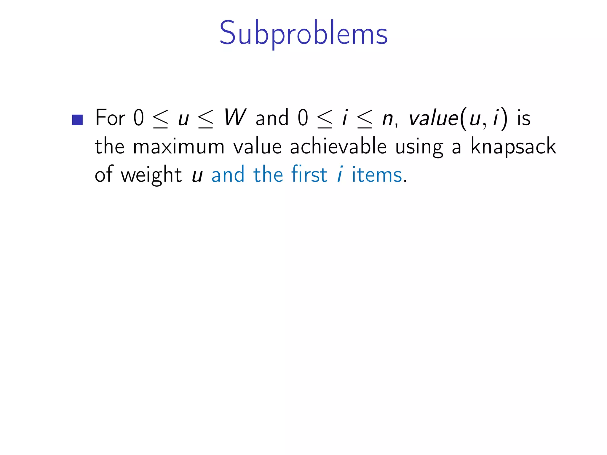
3 Knapsack: K(w) is the optimal value of
a knapsack of total weight w
4 Chain matrix multiplication M(i, j) is the
optimal cost of multiplying matrices through i
to j − 1](https://crownmelresort.com/image.slidesharecdn.com/dynamicprograming-220116082321/75/Dynamic-programing-264-2048.jpg)