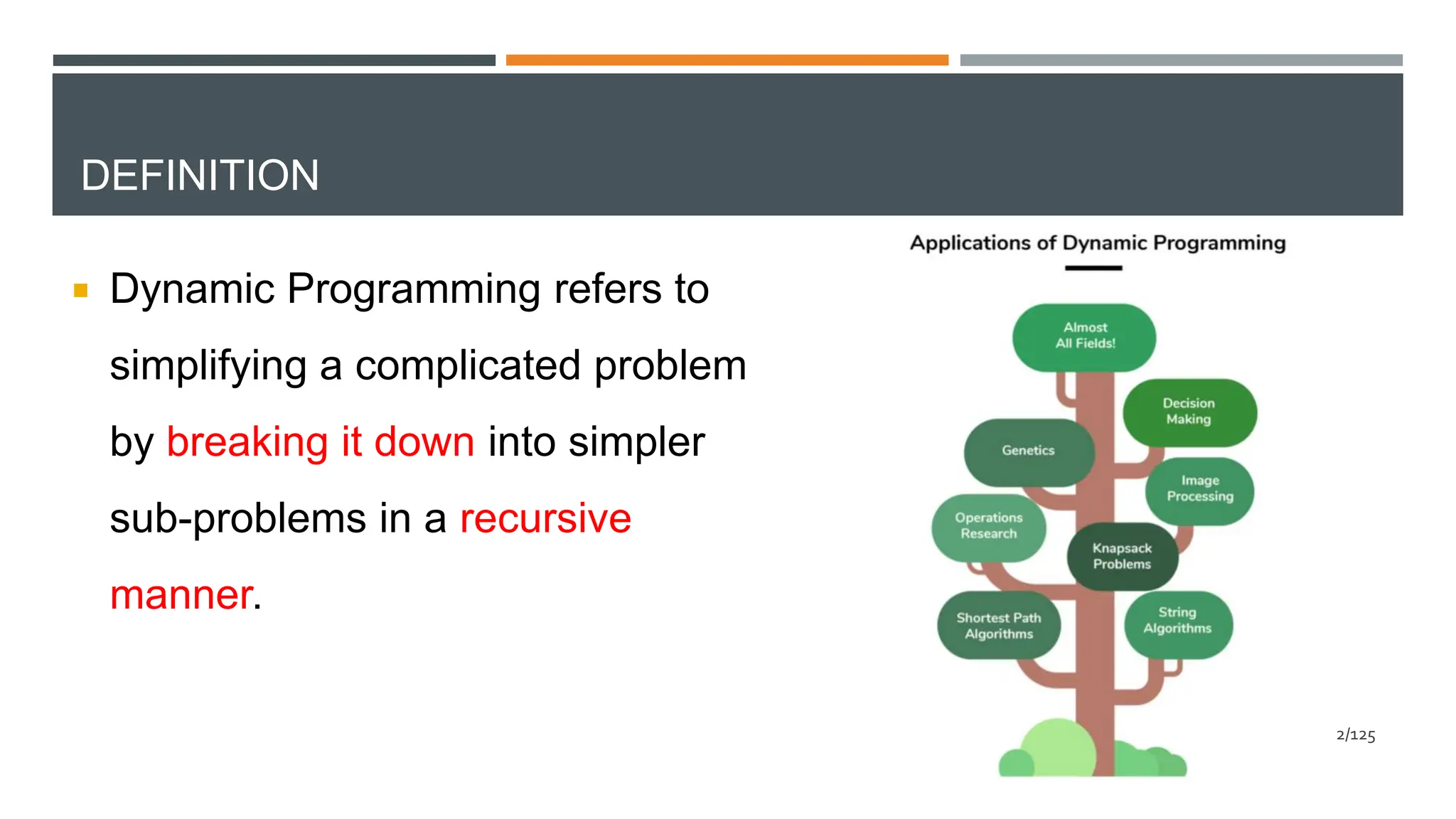
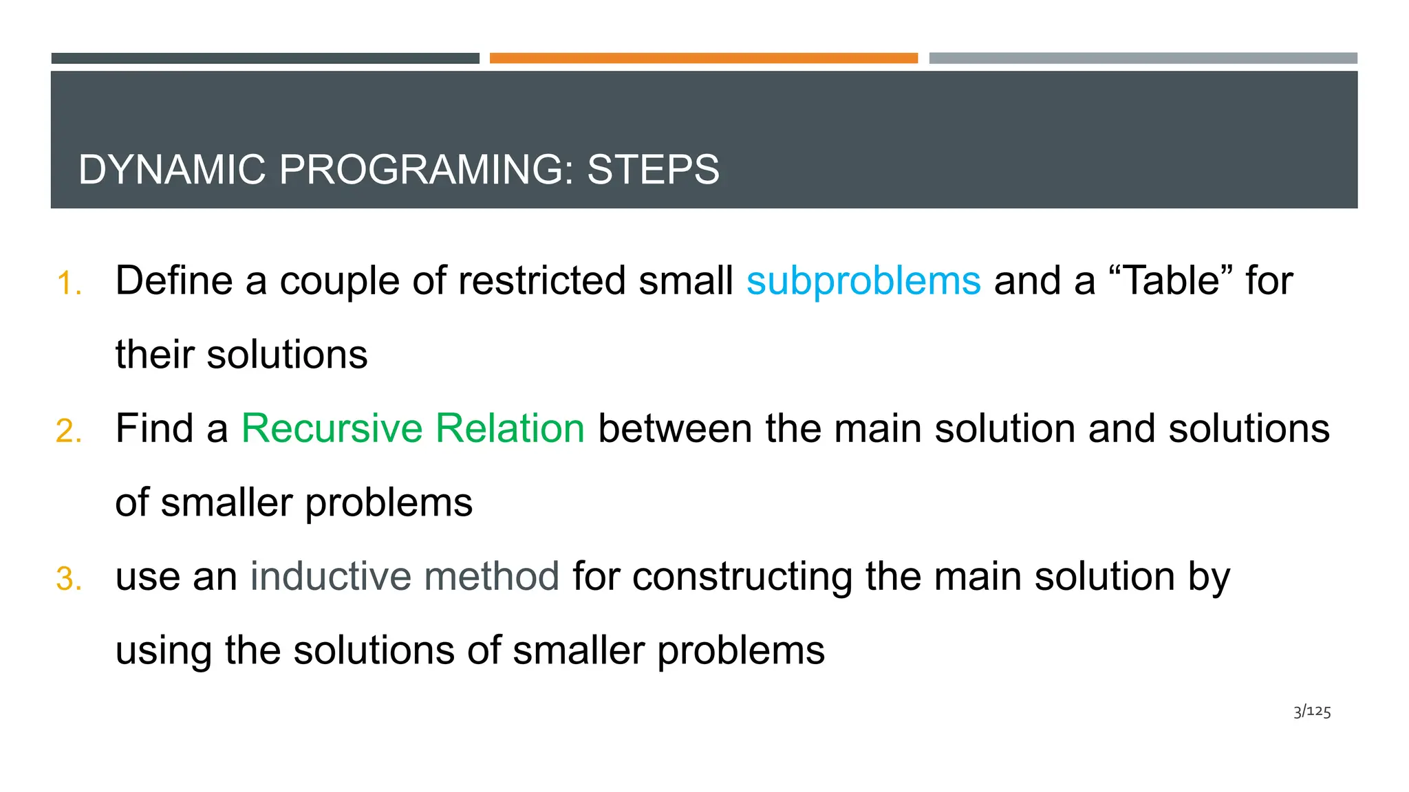
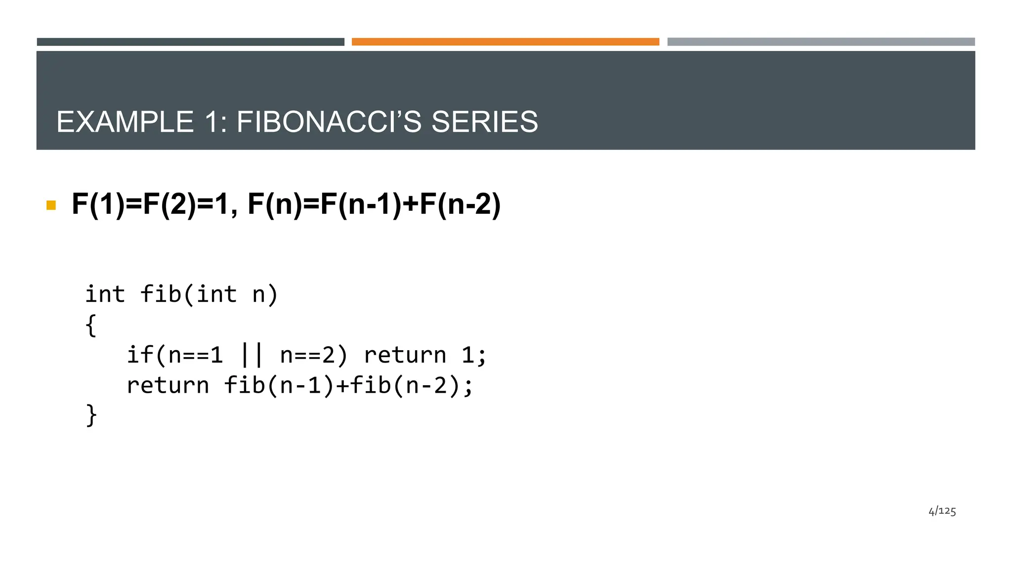
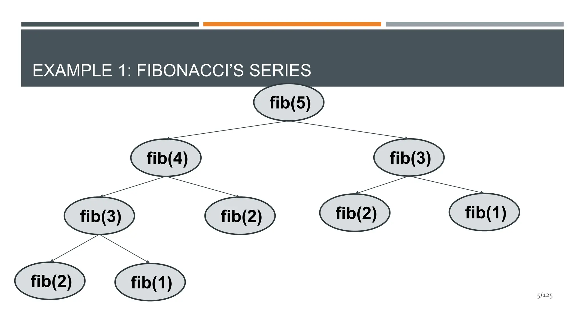
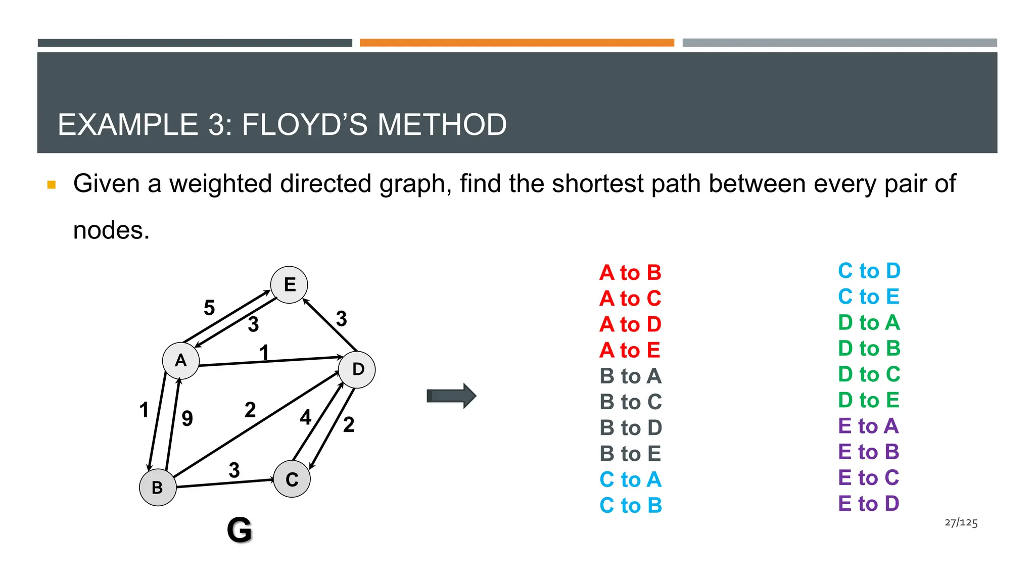
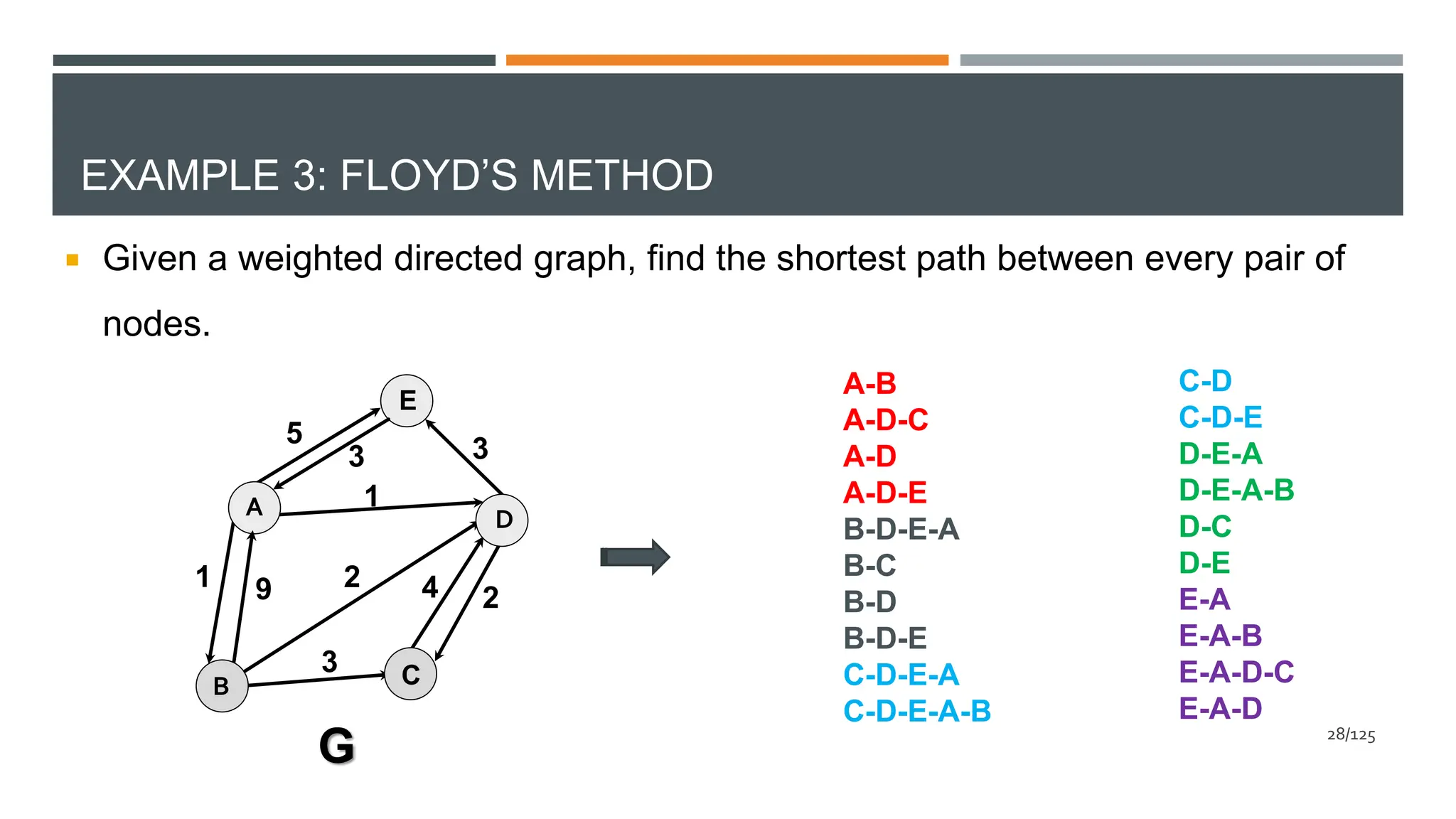
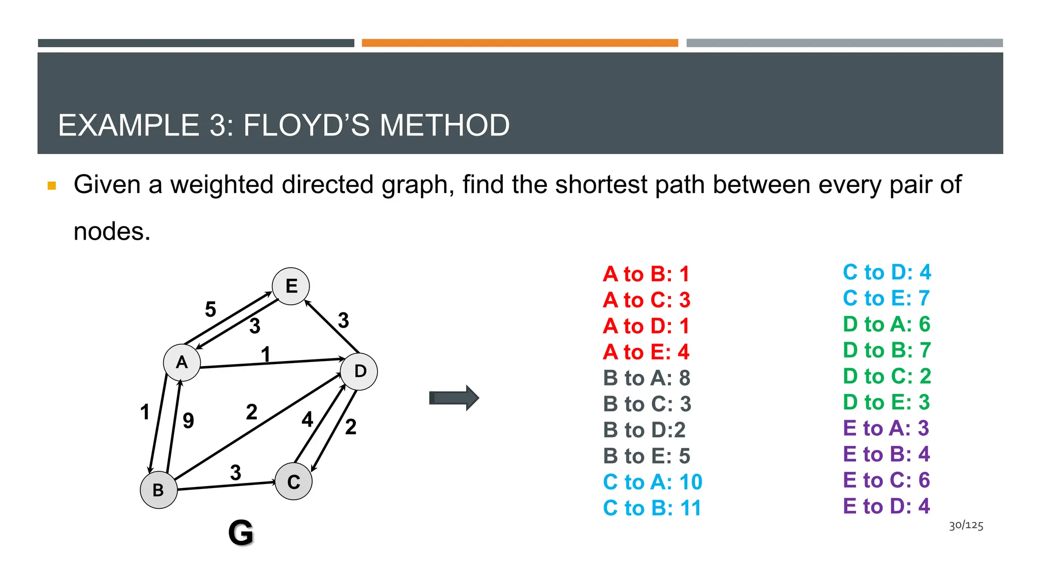
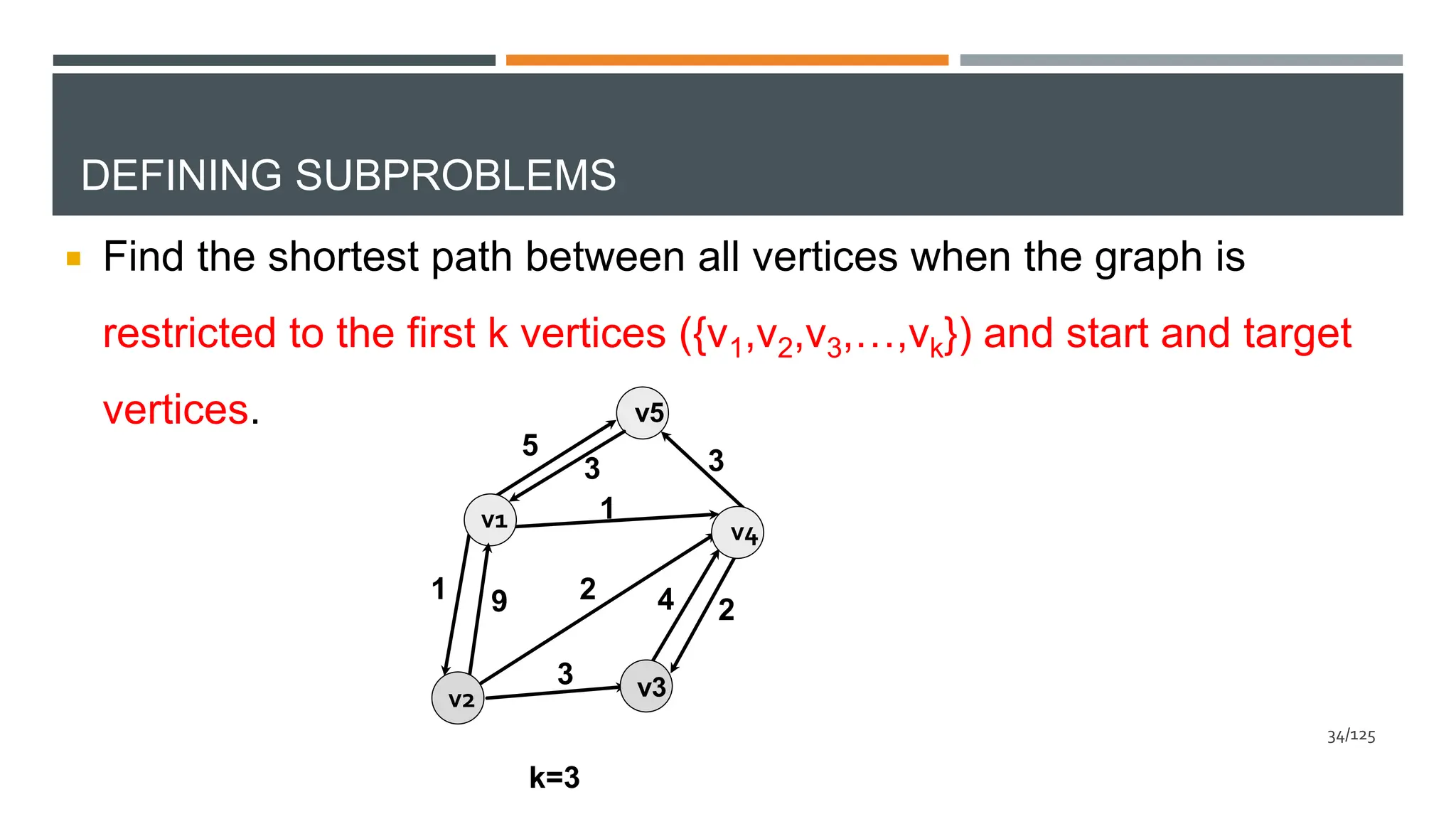
The document explains dynamic programming, a method for solving complex problems by breaking them down into simpler sub-problems, illustrated with examples such as the Fibonacci series and binomial coefficients. It details the steps involved in defining sub-problems, finding recursive relationships, and constructing solutions, along with time complexity analysis. Additionally, it covers Floyd's method for finding the shortest path in a weighted directed graph, providing an overview of how to represent graphs and analyze their shortest paths.

![FIBONACCI’S SERIES: DP APPROACH
fib(int n)
{
F[0]=F[1]=1;
for(i=2;i<=n;i++)
F[i]=F[i-1]+F[i-2];
}
1 - - - - -
1
F
1 2 - - - -
1
F
1 2 3 - - -
1
F
1 2 3 5 - -
1
F
fib(5)=?
- - - - - -
-
F
𝑂(𝑛)
7/125](https://image.slidesharecdn.com/dynamicprogramming-240626031018-00b06727/75/Data-Structures-and-algorithms-using-dynamicProgramming-7-2048.jpg)
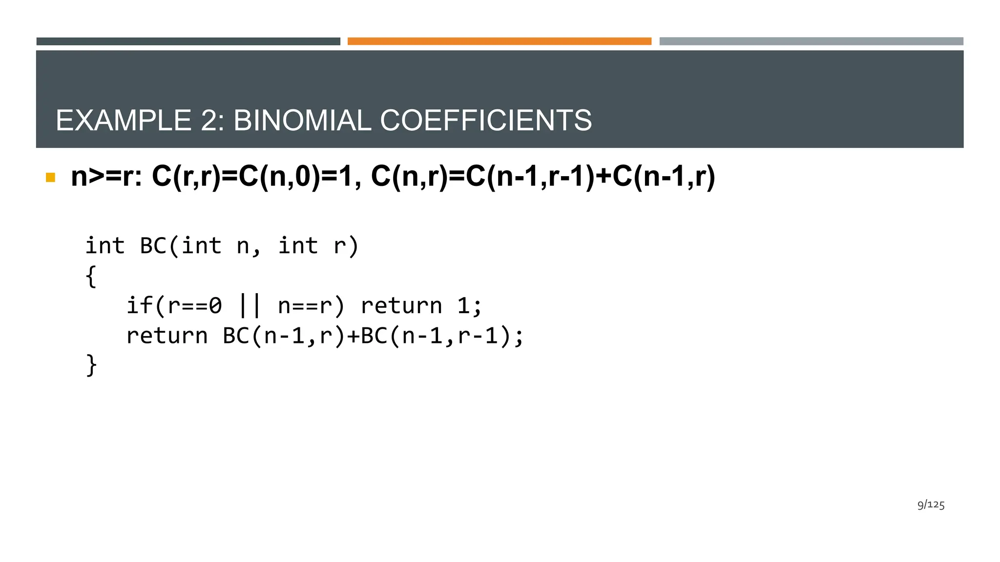
![EXAMPLE 2: BINOMIAL COEFFICIENT
int BC(int n, int r)
{
for(i=0;i<=n;i++)
for(j=0;j<=r;j++)
if(i>=j)
{
if(j==0 || i==j) M[i][j]=1;
else
M[i][j]=M[i-1][j]+M[i-1][j-1];
}
return M[n][r];
}
0
1
2
3
4
0 1 2 3
4
1
1 1
1 1
1 1
1 1
14/125
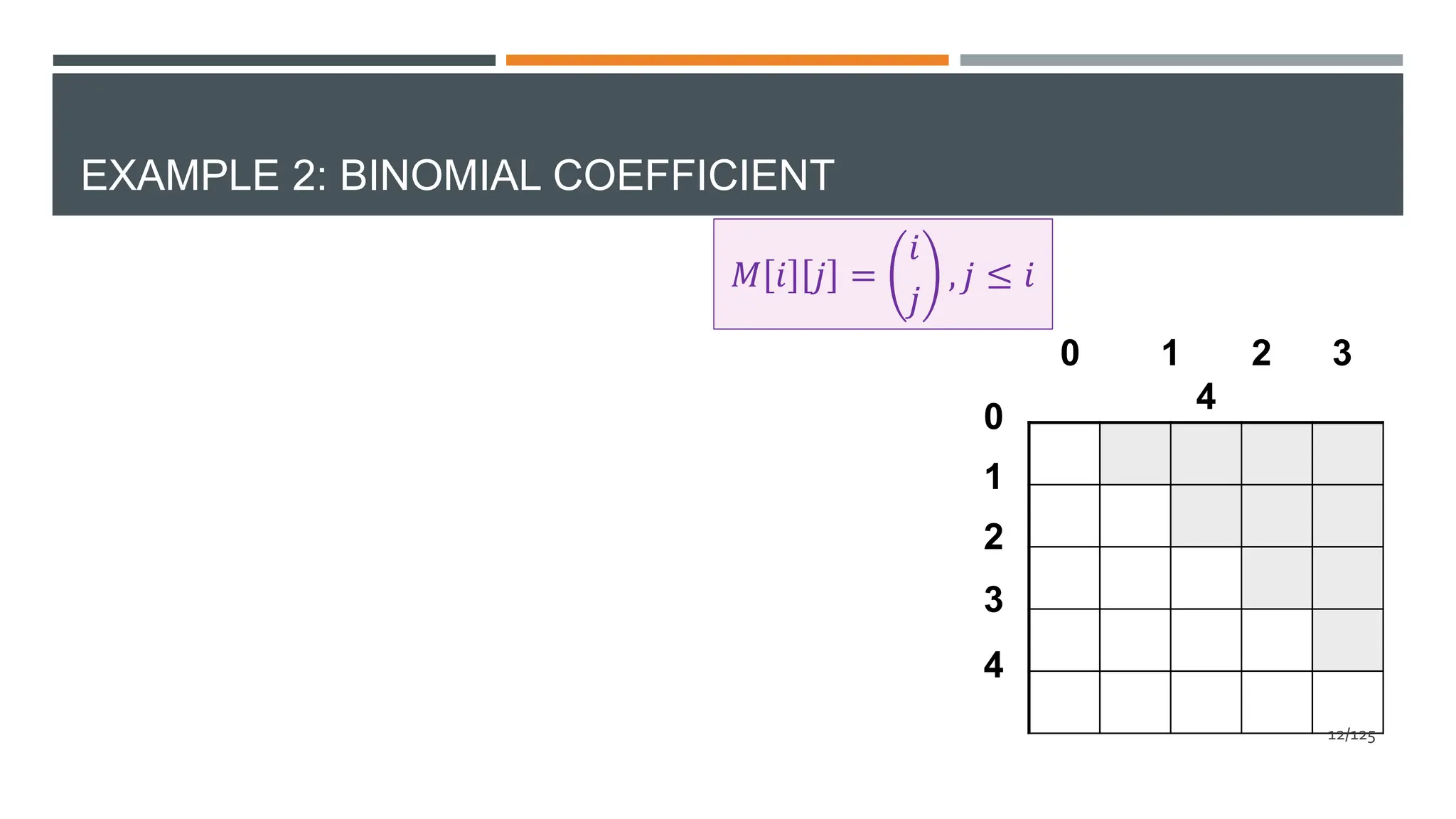
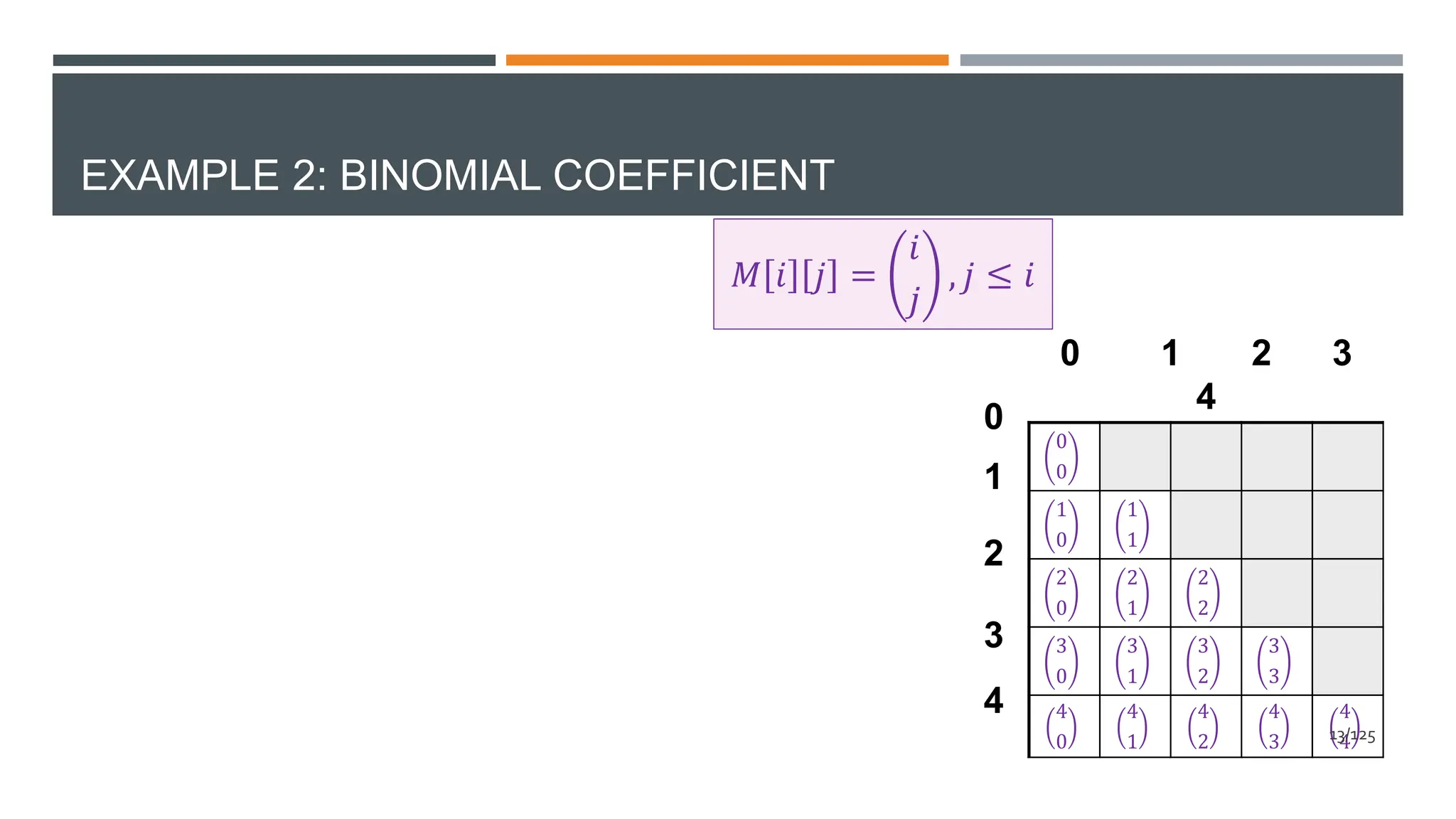
𝑀 𝑖 𝑗 =
𝑖
𝑗
, 𝑗 ≤ 𝑖](https://image.slidesharecdn.com/dynamicprogramming-240626031018-00b06727/75/Data-Structures-and-algorithms-using-dynamicProgramming-14-2048.jpg)
![EXAMPLE 2: BINOMIAL COEFFICIENT
int BC(int n, int r)
{
for(i=0;i<=n;i++)
for(j=0;j<=r;j++)
if(i>=j)
{
if(j==0 || i==j) M[i][j]=1;
else
M[i][j]=M[i-1][j]+M[i-1][j-1];
}
return M[n][r];
}
0
1
2
3
4
0 1 2 3
4
1
1 1
1 1
1 1
1 1
M[4][2]=? 15/125
𝑀 𝑖 𝑗 =
𝑖
𝑗
, 𝑗 ≤ 𝑖](https://image.slidesharecdn.com/dynamicprogramming-240626031018-00b06727/75/Data-Structures-and-algorithms-using-dynamicProgramming-15-2048.jpg)
![EXAMPLE 2: BINOMIAL COEFFICIENT
0
1
2
3
4
0 1 2 3
4
1
1 1
1 1
1 1
1 1
M[2][1]=?
16/125](https://image.slidesharecdn.com/dynamicprogramming-240626031018-00b06727/75/Data-Structures-and-algorithms-using-dynamicProgramming-16-2048.jpg)
![EXAMPLE 2: BINOMIAL COEFFICIENT
0
1
2
3
4
0 1 2 3
4
1
1 1
1 2 1
1 1
1 1
M[2][1]=?
17/125](https://image.slidesharecdn.com/dynamicprogramming-240626031018-00b06727/75/Data-Structures-and-algorithms-using-dynamicProgramming-17-2048.jpg)
![EXAMPLE 2: BINOMIAL COEFFICIENT
0
1
2
3
4
0 1 2 3
4
1
1 1
1 2 1
1 1
1 1
M[3][1]=?
18/125](https://image.slidesharecdn.com/dynamicprogramming-240626031018-00b06727/75/Data-Structures-and-algorithms-using-dynamicProgramming-18-2048.jpg)
![EXAMPLE 2: BINOMIAL COEFFICIENT
0
1
2
3
4
0 1 2 3
4
1
1 1
1 2 1
1 3 1
1 1
M[3][1]=?
19/125](https://image.slidesharecdn.com/dynamicprogramming-240626031018-00b06727/75/Data-Structures-and-algorithms-using-dynamicProgramming-19-2048.jpg)
![EXAMPLE 2: BINOMIAL COEFFICIENT
0
1
2
3
4
0 1 2 3
4
1
1 1
1 2 1
1 3 1
1 1
M[3][2]=?
20/125](https://image.slidesharecdn.com/dynamicprogramming-240626031018-00b06727/75/Data-Structures-and-algorithms-using-dynamicProgramming-20-2048.jpg)
![EXAMPLE 2: BINOMIAL COEFFICIENT
0
1
2
3
4
0 1 2 3
4
1
1 1
1 2 1
1 3 3 1
1 1
M[3][2]=?
21/125](https://image.slidesharecdn.com/dynamicprogramming-240626031018-00b06727/75/Data-Structures-and-algorithms-using-dynamicProgramming-21-2048.jpg)
![EXAMPLE 2: BINOMIAL COEFFICIENT
0
1
2
3
4
0 1 2 3
4
1
1 1
1 2 1
1 3 3 1
1 1
M[4][1]=?
22/125](https://image.slidesharecdn.com/dynamicprogramming-240626031018-00b06727/75/Data-Structures-and-algorithms-using-dynamicProgramming-22-2048.jpg)
![EXAMPLE 2: BINOMIAL COEFFICIENT
0
1
2
3
4
0 1 2 3
4
1
1 1
1 2 1
1 3 3 1
1 4 1
M[4][1]=?
23/125](https://image.slidesharecdn.com/dynamicprogramming-240626031018-00b06727/75/Data-Structures-and-algorithms-using-dynamicProgramming-23-2048.jpg)
![EXAMPLE 2: BINOMIAL COEFFICIENT
0
1
2
3
4
0 1 2 3
4
1
1 1
1 2 1
1 3 3 1
1 4 1
M[4][2]=?
24/125](https://image.slidesharecdn.com/dynamicprogramming-240626031018-00b06727/75/Data-Structures-and-algorithms-using-dynamicProgramming-24-2048.jpg)
![EXAMPLE 2: BINOMIAL COEFFICIENT
0
1
2
3
4
0 1 2 3
4
1
1 1
1 2 1
1 3 3 1
1 4 6 1
M[4][2]=?
25/125](https://image.slidesharecdn.com/dynamicprogramming-240626031018-00b06727/75/Data-Structures-and-algorithms-using-dynamicProgramming-25-2048.jpg)
![BINOMIAL COEFFICIENT: TIME COMPLEXITY
int BC(int n, int r)
{
for(i=0;i<=n;i++)
for(j=0;j<=r;j++)
if(i>=j)
{
if(j==0 || i==j) M[i][j]=1;
else
M[i][j]=M[i-1][j]+M[i-1][j-1];
}
return M[n][r];
}
26/125
𝑂(𝑛𝑟)](https://image.slidesharecdn.com/dynamicprogramming-240626031018-00b06727/75/Data-Structures-and-algorithms-using-dynamicProgramming-26-2048.jpg)

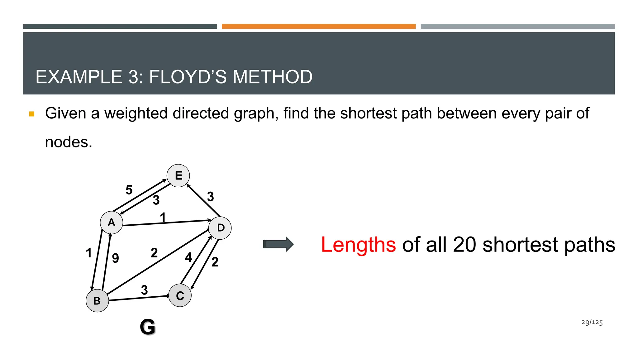
![GRAPH: REPRESENTATION
A D
C
E
G
B
1
1
5
9
3
2 4 2
3
3
A B C D E
A 0 1
8
1 5
B 9 0 3 2
8
C
8
8
0 4
8
D
8
8
2 0 3
E 3
8
8
8
0
W
31/125
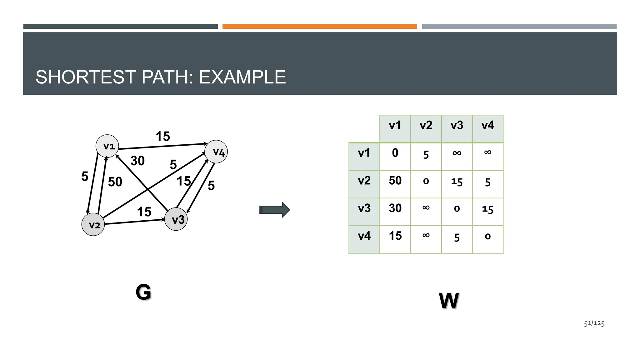
W[i][j]=weight of edge from vertex i to j](https://image.slidesharecdn.com/dynamicprogramming-240626031018-00b06727/75/Data-Structures-and-algorithms-using-dynamicProgramming-31-2048.jpg)
![SHORTEST PATHS: REPRESENTATION
A D
C
E
G
B
1
1
5
9
3
2 4 2
3
3
A B C D E
A 0 1 3 1 4
B 8 0 3 2 5
C 10 11 0 4 7
D 6 7 2 0 3
E 3 4 6 4 0
D
32/125
D[i][j]=length of shortest path from vertex i to j](https://image.slidesharecdn.com/dynamicprogramming-240626031018-00b06727/75/Data-Structures-and-algorithms-using-dynamicProgramming-32-2048.jpg)


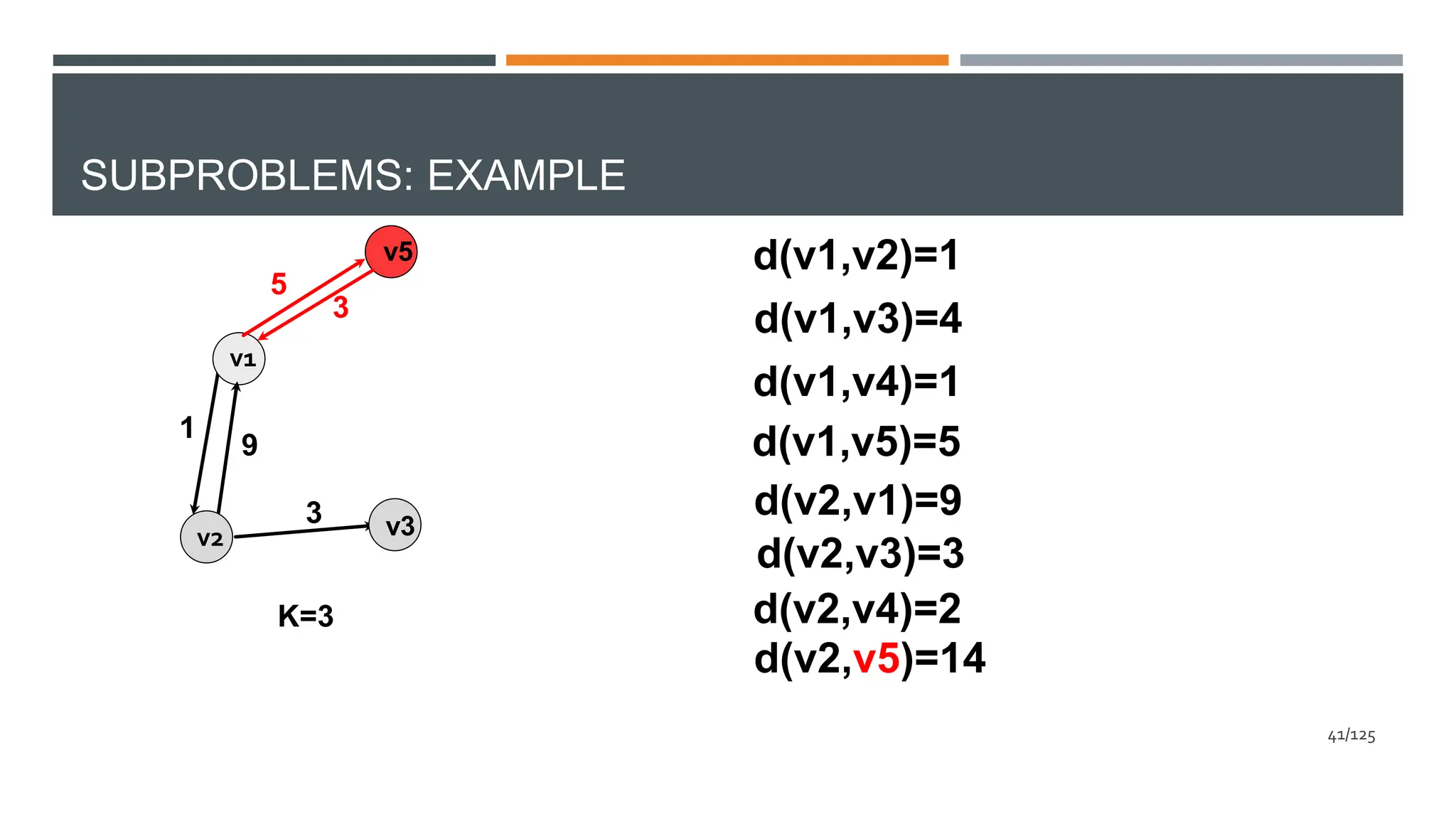


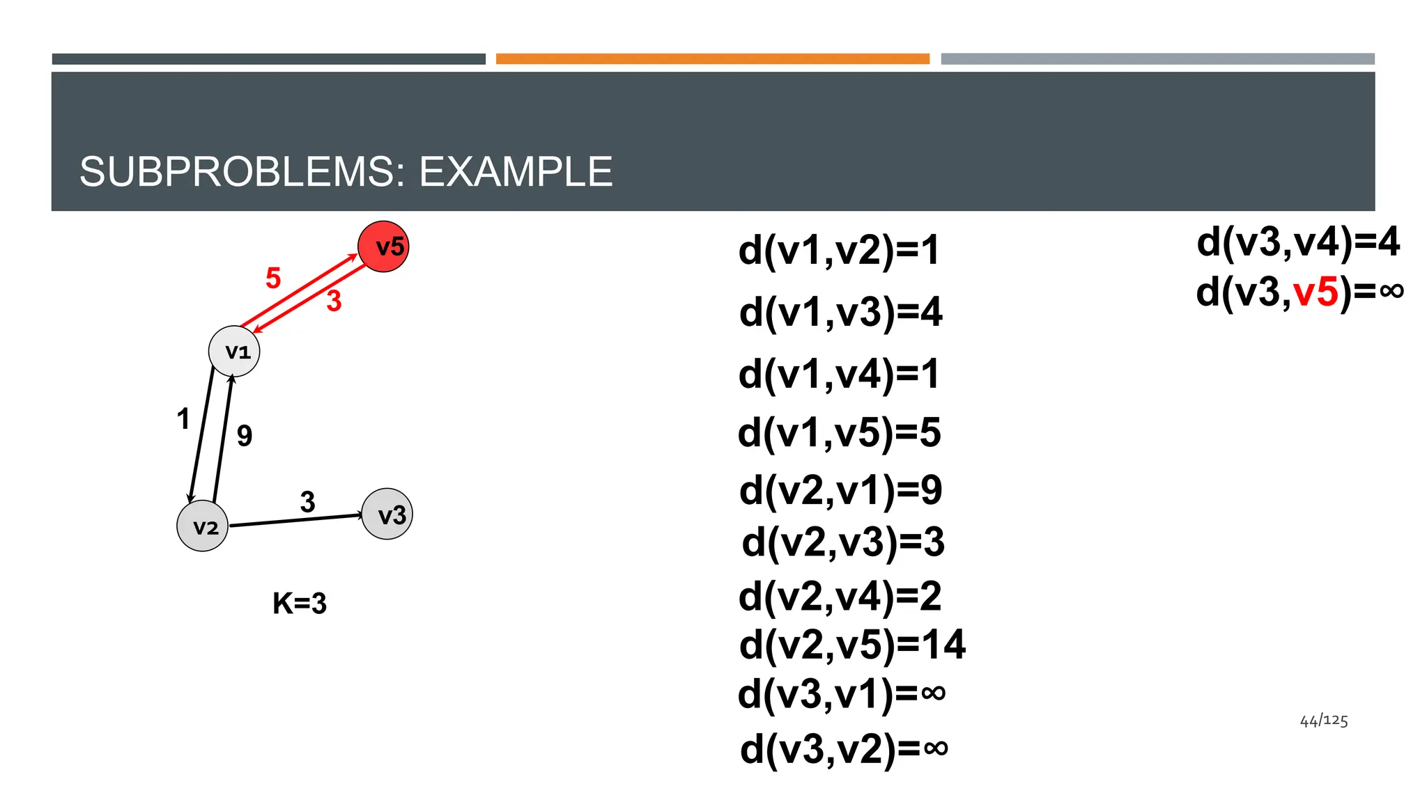
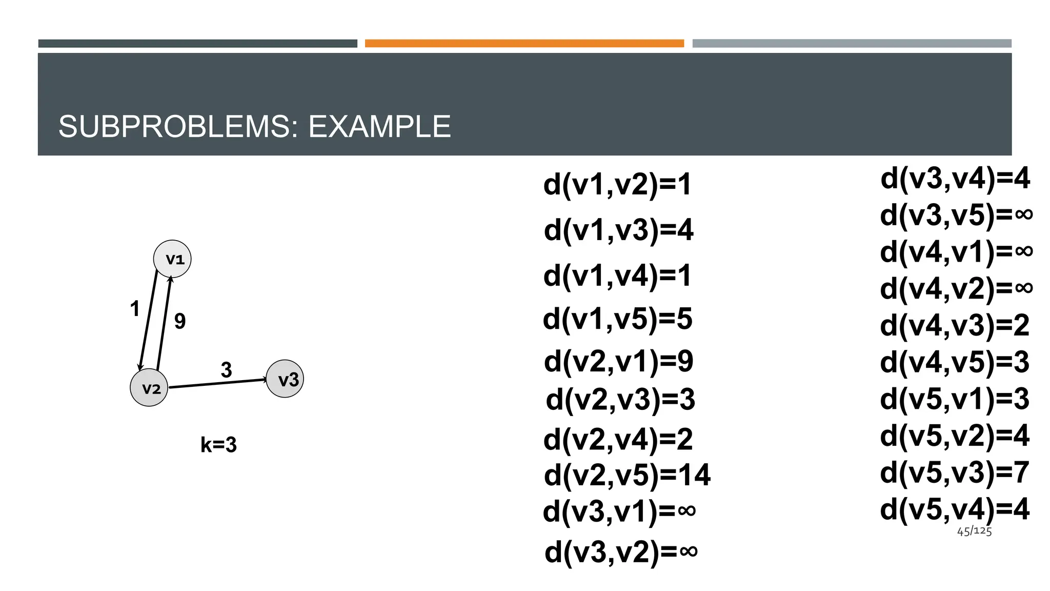
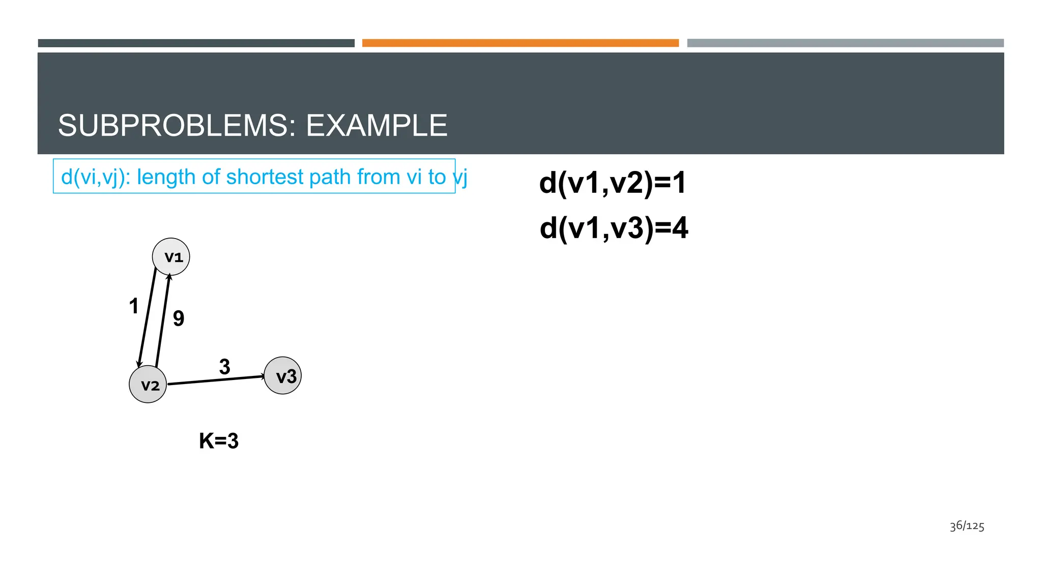
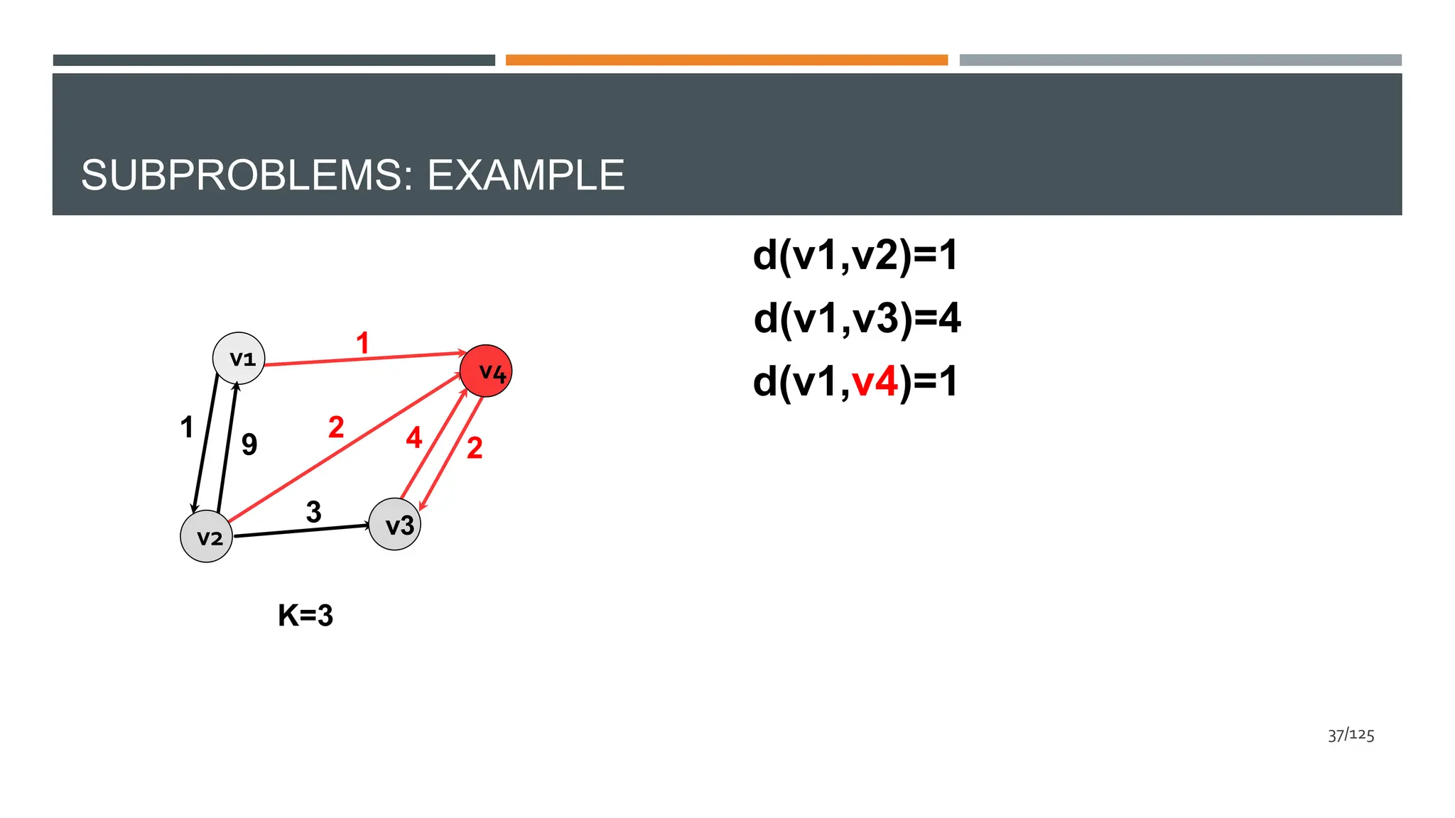
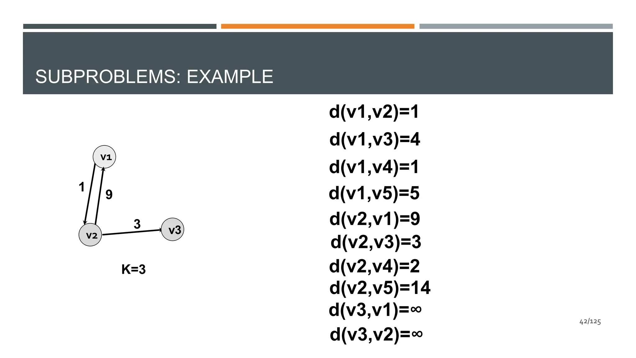
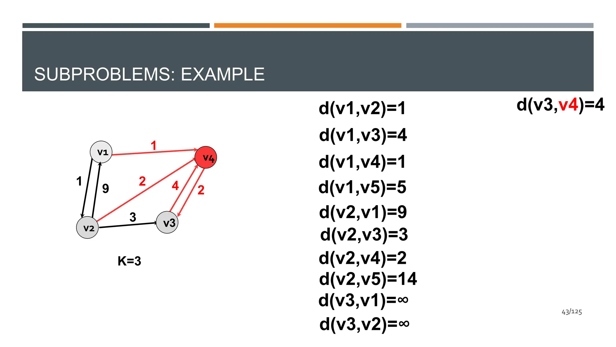
![SUBPROBLEMS: REPRESENTATION
v1 v4
v3
v5
v2
1
1
5
9
3
2 4 2
3
3
v1 v2 v3 v4 v5
v1 0 1 4 1 5
v2 9 0 3 2 14
v3 ∞ ∞ 0 4 ∞
v4 ∞ ∞ 2 0 3
v5 3 4 7 4 0
D
(3)
D [i][j]=length of shortest path between vi and vj in
the graph restricted to vertices {v1,v2,…,vk}
(k)
46/125](https://image.slidesharecdn.com/dynamicprogramming-240626031018-00b06727/75/Data-Structures-and-algorithms-using-dynamicProgramming-46-2048.jpg)
![CALCULATING DS
vi vj
D [i][j]
(k+1)
48/125](https://image.slidesharecdn.com/dynamicprogramming-240626031018-00b06727/75/Data-Structures-and-algorithms-using-dynamicProgramming-48-2048.jpg)
![CALCULATING DS
vi vj
D [i][j]
(k+1)
vi vj
vi vj
Vk+1
49/125](https://image.slidesharecdn.com/dynamicprogramming-240626031018-00b06727/75/Data-Structures-and-algorithms-using-dynamicProgramming-49-2048.jpg)
![CALCULATING DS
vi vj
D [i][j]
(k+1)
vi vj
vi vj
Vk+1
D(k)[i][j]
D [i][k+1]+D [k+1][j]
(k) (k)
D [i][k+1]+D [k+1][j],
(k) (k)
D [i][j]=min{
(k+1)
D [i][j]}
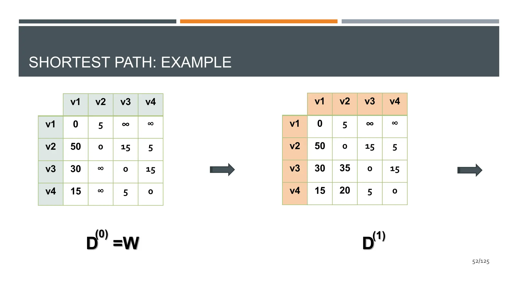
(k) 50/125](https://image.slidesharecdn.com/dynamicprogramming-240626031018-00b06727/75/Data-Structures-and-algorithms-using-dynamicProgramming-50-2048.jpg)

![FLOYD’S METHOD: ALGORITHM
Floyd(int W[][], int n)
{
D=W;//initializing D0
for(k=1;k<=n;k++) //calculating Dk
for(i=1;i<=n;i++)
for(j=1;j<=n;j++)
D[i][j]=min{D[i][j],D[i][k]+D[k][j]};
return D;
}
𝑂(𝑛3
)
55/125](https://image.slidesharecdn.com/dynamicprogramming-240626031018-00b06727/75/Data-Structures-and-algorithms-using-dynamicProgramming-55-2048.jpg)
![FLOYD’S METHOD: ALGORITHM
Floyd(int W[][], int n)
{
D=W;//initializing D0
for(k=1;k<=n;k++) //calculating Dk
for(i=1;i<=n;i++)
for(j=1;j<=n;j++)
if(D[i][k]+D[k][j]<D[i][j])
D[i][j]=D[i][k]+D[k][j];
return D;
}
𝑂(𝑛3
)
56/125](https://image.slidesharecdn.com/dynamicprogramming-240626031018-00b06727/75/Data-Structures-and-algorithms-using-dynamicProgramming-56-2048.jpg)
![SHORTEST PATHS!
Rows and columns of P: v1 to vn
P[i][j]=r: shortest path from vi to vj passes through vr
P[i][j]=0: edge vivj is the shortest path from vi to vj
1. How can I calculate P?
2. How can I use P for finding shortest paths?
57/125](https://image.slidesharecdn.com/dynamicprogramming-240626031018-00b06727/75/Data-Structures-and-algorithms-using-dynamicProgramming-57-2048.jpg)
![SHORTEST PATHS!
P[i][j]=r: shortest path from vi to vj passes through vr
P[i][j]=0: edge vivj is the shortest path from vi to vj
v1 v2 v3 v4
v1 0 0 4 2
v2 4 0 4 0
v3 0 1 0 0
v4 0 1 0 0
P
58/125](https://image.slidesharecdn.com/dynamicprogramming-240626031018-00b06727/75/Data-Structures-and-algorithms-using-dynamicProgramming-58-2048.jpg)
![SHORTEST PATHS!
v1 v2 v3 v4
v1 0 0 4 2
v2 4 0 4 0
v3 0 1 0 0
v4 0 1 0 0
P
SP(v1,v3)=?? v1 v3
59/125
P[i][j]=r: shortest path from vi to vj passes through vr
P[i][j]=0: edge vivj is the shortest path from vi to vj](https://image.slidesharecdn.com/dynamicprogramming-240626031018-00b06727/75/Data-Structures-and-algorithms-using-dynamicProgramming-59-2048.jpg)
![SHORTEST PATHS!
v1 v2 v3 v4
v1 0 0 4 2
v2 4 0 4 0
v3 0 1 0 0
v4 0 1 0 0
P
SP(v1,v3)=??
P[v1][v3]=4
v1 v3
v4
60/125
P[i][j]=r: shortest path from vi to vj passes through vr
P[i][j]=0: edge vivj is the shortest path from vi to vj](https://image.slidesharecdn.com/dynamicprogramming-240626031018-00b06727/75/Data-Structures-and-algorithms-using-dynamicProgramming-60-2048.jpg)
![SHORTEST PATHS!
v1 v2 v3 v4
v1 0 0 4 2
v2 4 0 4 0
v3 0 1 0 0
v4 0 1 0 0
P
SP(v1,v3)=??
P[v1][v3]=4
1. SP(v1,v4)=?
2. SP(v4,v3)=?
v1 v3
v4
61/125
P[i][j]=r: shortest path from vi to vj passes through vr
P[i][j]=0: edge vivj is the shortest path from vi to vj](https://image.slidesharecdn.com/dynamicprogramming-240626031018-00b06727/75/Data-Structures-and-algorithms-using-dynamicProgramming-61-2048.jpg)
![SHORTEST PATHS!
v1 v2 v3 v4
v1 0 0 4 2
v2 4 0 4 0
v3 0 1 0 0
v4 0 1 0 0
P
SP(v1,v3)=??
P[v1][v3]=4
1. P[v1][v4]=?
2. P[v4][v3]=?
v1 v3
v4
62/125
P[i][j]=r: shortest path from vi to vj passes through vr
P[i][j]=0: edge vivj is the shortest path from vi to vj](https://image.slidesharecdn.com/dynamicprogramming-240626031018-00b06727/75/Data-Structures-and-algorithms-using-dynamicProgramming-62-2048.jpg)
![SHORTEST PATHS!
v1 v2 v3 v4
v1 0 0 4 2
v2 4 0 4 0
v3 0 1 0 0
v4 0 1 0 0
P
SP(v1,v3)=??
P[v1][v3]=4
1. P[v1][v4]=2
2. P[v4][v3]=0
v1 v3
v4
63/125
P[i][j]=r: shortest path from vi to vj passes through vr
P[i][j]=0: edge vivj is the shortest path from vi to vj](https://image.slidesharecdn.com/dynamicprogramming-240626031018-00b06727/75/Data-Structures-and-algorithms-using-dynamicProgramming-63-2048.jpg)
![SHORTEST PATHS!
v1 v2 v3 v4
v1 0 0 4 2
v2 4 0 4 0
v3 0 1 0 0
v4 0 1 0 0
P
SP(v1,v3)=??
P[v1][v3]=4
1. P[v1][v4]=2
2. P[v4][v3]=0
v1
v2
64/125
v4
v3
P[i][j]=r: shortest path from vi to vj passes through vr
P[i][j]=0: edge vivj is the shortest path from vi to vj](https://image.slidesharecdn.com/dynamicprogramming-240626031018-00b06727/75/Data-Structures-and-algorithms-using-dynamicProgramming-64-2048.jpg)
![SHORTEST PATHS!
v1 v2 v3 v4
v1 0 0 4 2
v2 4 0 4 0
v3 0 1 0 0
v4 0 1 0 0
P
SP(v1,v3)=??
P[v1][v3]=4
1. P[v1][v4]=2
1.1. P[v1][v2]=0
1.2. P[v2][v4]=0
2. P[v4][v3]=0
v1
v2
65/125
v3
v4
P[i][j]=r: shortest path from vi to vj passes through vr
P[i][j]=0: edge vivj is the shortest path from vi to vj](https://image.slidesharecdn.com/dynamicprogramming-240626031018-00b06727/75/Data-Structures-and-algorithms-using-dynamicProgramming-65-2048.jpg)
![SHORTEST PATHS!
v1 v2 v3 v4
v1 0 0 4 2
v2 4 0 4 0
v3 0 1 0 0
v4 0 1 0 0
P
SP(v1,v3)=??
P[v1][v3]=4
1. P[v1][v4]=2
1.1. P[v1][v2]=0
1.2. P[v2][v4]=0
2. P[v4][v3]=0
v2
66/125
v3
v4
v1
P[i][j]=r: shortest path from vi to vj passes through vr
P[i][j]=0: edge vivj is the shortest path from vi to vj](https://image.slidesharecdn.com/dynamicprogramming-240626031018-00b06727/75/Data-Structures-and-algorithms-using-dynamicProgramming-66-2048.jpg)
![CALCULATING P
vi vj
D [i][j]
(k+1)
vi vj
vi vj
Vk+1
P[i][j]=k+1
D [i][k+1]+D [k+1][j] : P[i][j]=k+1
(k) (k)
If D [i][j]=
(k+1) 67/125](https://image.slidesharecdn.com/dynamicprogramming-240626031018-00b06727/75/Data-Structures-and-algorithms-using-dynamicProgramming-67-2048.jpg)
![FLOYD’S ALGORITHM
Floyd(int W[][], int n){
D=W;
P=0;
for(k=1;k<=n;k++)
for(i=1;i<=n;i++)
for(j=1;j<=n;j++)
if(D[i][k]+D[k][j]<D[i][j])
{
D[i][j]=D[i][k]+D[k][j];
P[i][j]=k+1;
}
return D;
}
68/125](https://image.slidesharecdn.com/dynamicprogramming-240626031018-00b06727/75/Data-Structures-and-algorithms-using-dynamicProgramming-68-2048.jpg)


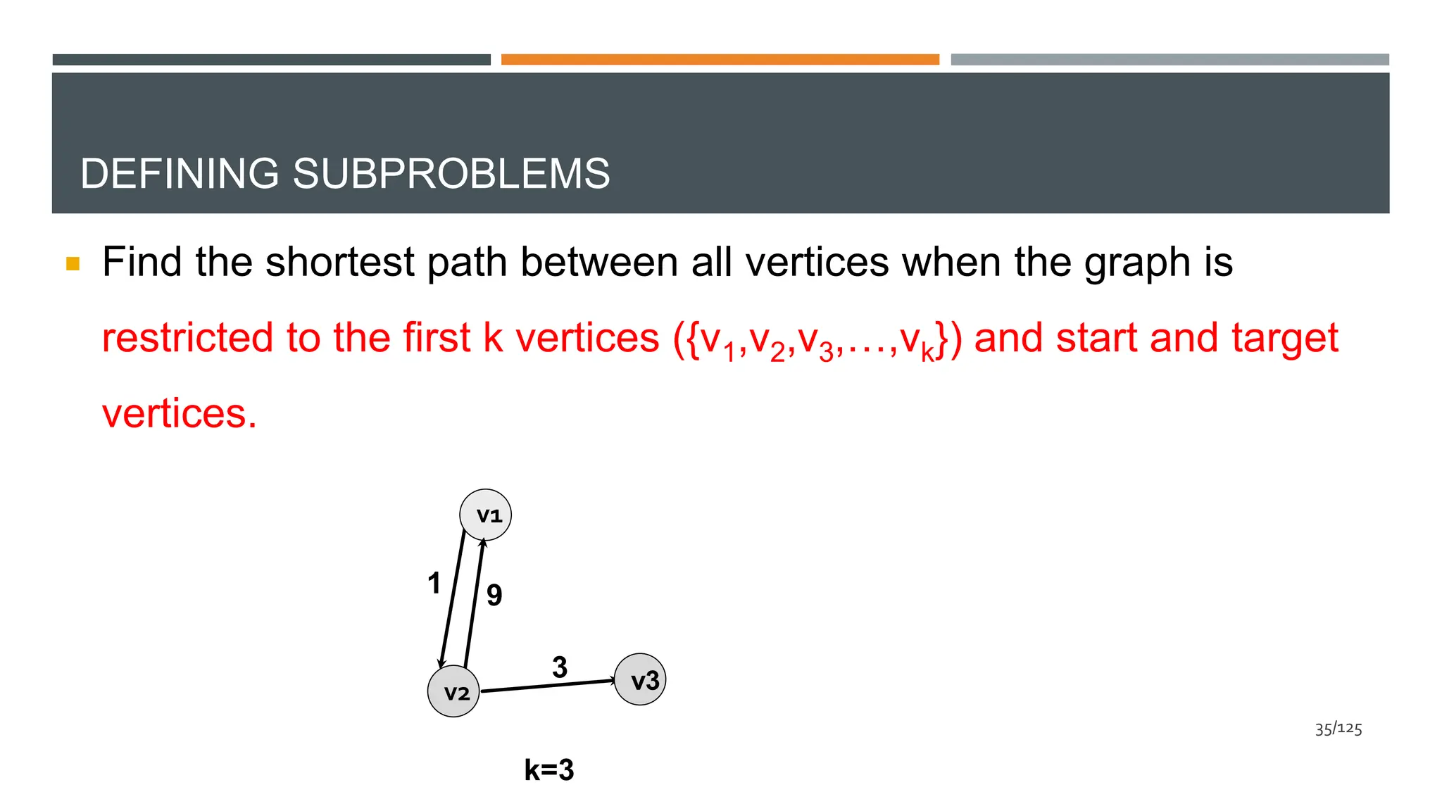
![DEFINING SUBPROBLEMS
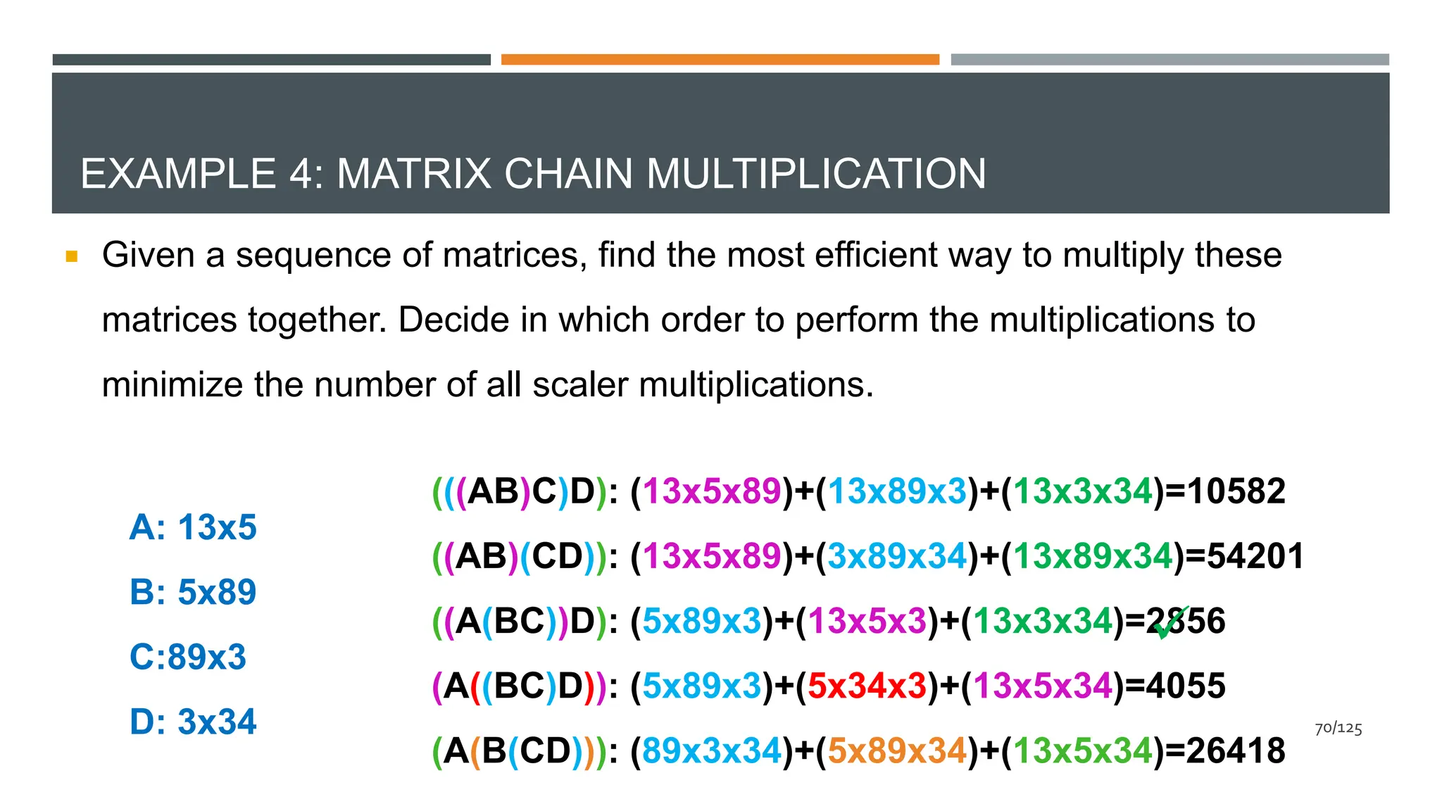
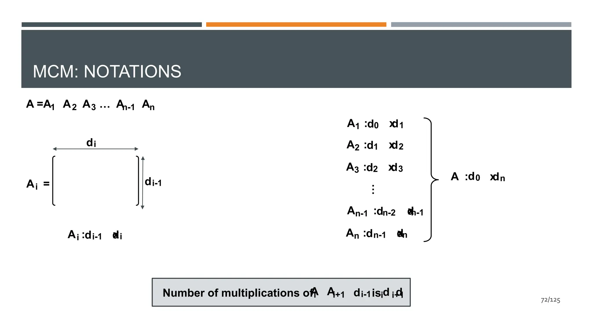
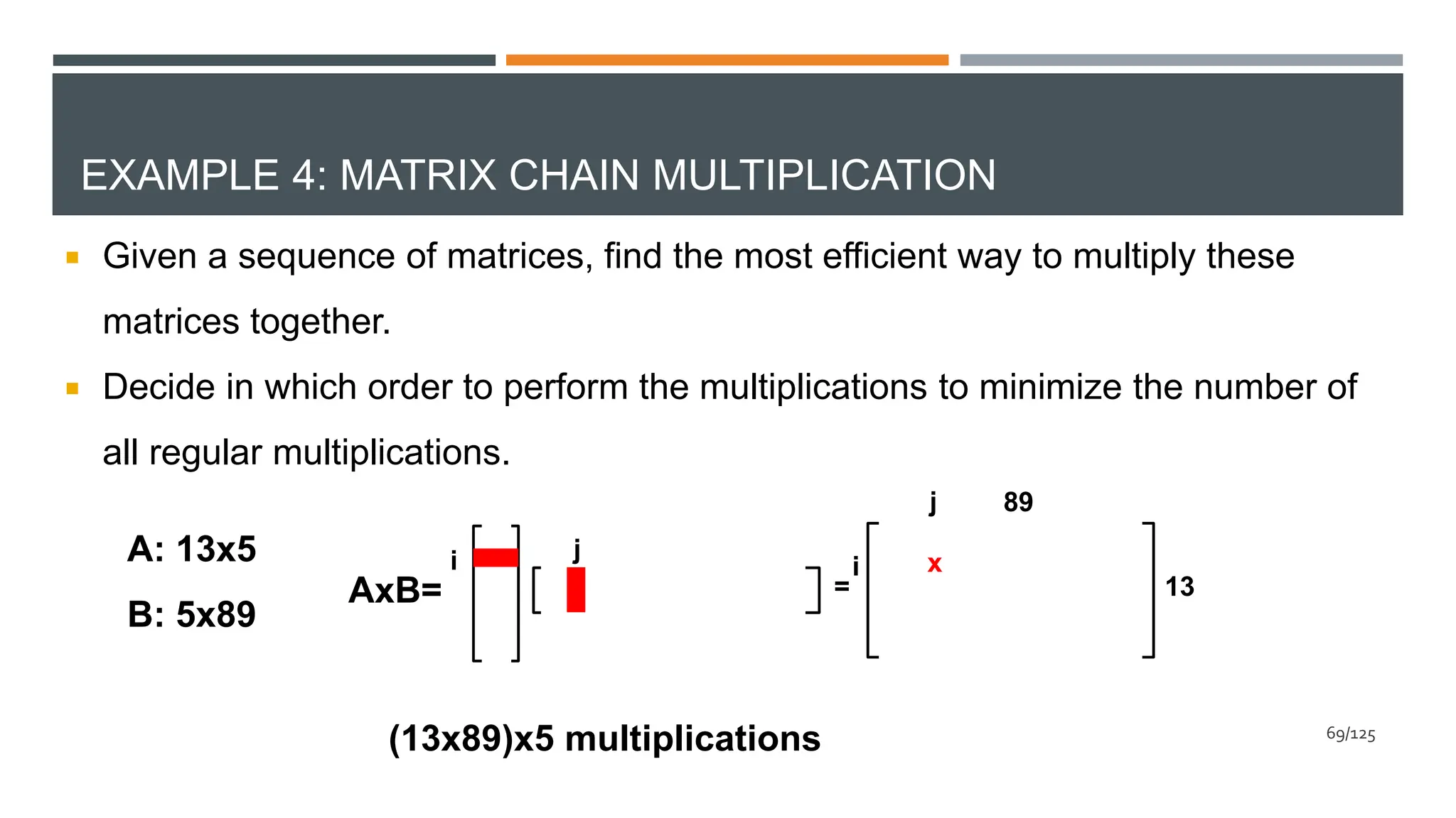
Find the most efficient way to multiply the following matrices
together:
For i>=j, M[i][j]=0
M[1][n]=Optimum number of multiplications.
A x A x … x A
i i+1 j
M[i][j]=Minimum number of multiplications
in product Ai Ai+1 … Aj , i<j
74/125](https://image.slidesharecdn.com/dynamicprogramming-240626031018-00b06727/75/Data-Structures-and-algorithms-using-dynamicProgramming-74-2048.jpg)
![CALCULATING M[I][J] A A … A
i i+1 j
d d
j
di-1 i
M[i+1][j]+
d d
j
di-1 i+1
M[i][i+1]+M[i+2][j]+
d d
j
di-1 i+2
M[i][i+2]+M[i+3][j]+
d d
j
di-1 k
M[i][k]+M[k+1][j]+
…
…
d d
j
di-1 j-3
M[i][j-3]+M[j-2][j]+
d d
j
di-1 j-2
M[i][j-2]+M[j-1][j]+
d d
j
di-1 j-1
M[i][j-1]+
(A … A )(A … A )
i i+2 i+3 j
(A … A )(A … A )
i j-3 j-2 j
(A A )(A … A )
i i+1 i+2 j
A (A … A )
i i+1 j
…
(A … A )(A … A )
i k k+1 j
…
(A … A )(A A )
i j-2 j-1 j
(A … A ) A
i j-1 j
MIN
75/125](https://image.slidesharecdn.com/dynamicprogramming-240626031018-00b06727/75/Data-Structures-and-algorithms-using-dynamicProgramming-75-2048.jpg)
![CALCULATING M[I][J]
A A … A
i i+1 j
(A … A )(A … A )
i k k+1 j
d d
j
di-1 k
M[i][j]= MIN { M[i][k]+M[k+1][j] + }
i<=k<j
MIN
M[i][i]= 0 76/125](https://image.slidesharecdn.com/dynamicprogramming-240626031018-00b06727/75/Data-Structures-and-algorithms-using-dynamicProgramming-76-2048.jpg)
![CALCULATING M
1
2
3
4
:
n
1 2 3 4
…
n
M[i][j]=?
A A … A
i i+1 j
77/125](https://image.slidesharecdn.com/dynamicprogramming-240626031018-00b06727/75/Data-Structures-and-algorithms-using-dynamicProgramming-77-2048.jpg)
![CALCULATING M
M[i][j]=?
A A … A
i i+1 j
i<=j 1
2
3
4
:
n
1 2 3 4
…
n
78/125](https://image.slidesharecdn.com/dynamicprogramming-240626031018-00b06727/75/Data-Structures-and-algorithms-using-dynamicProgramming-78-2048.jpg)
![CALCULATING M
Diagonal 0
Diagonal 1
Diagonal 2
Diagonal n-2
Diagonal n-1
M[i][i]: n
M[i][i+1]: n-1
M[i][i+2]: n-2
M[i][i+d]: n-d
M[i][i+n-2]: 2
M[1][1+n-1]: 1
Diagonal d: M[i][i+d], 1<=i<=n-d M[i][j] lies on Diagonal j-i
1
2
3
4
:
n
1 2 3 4
…
n
Diagonal d
79/125](https://image.slidesharecdn.com/dynamicprogramming-240626031018-00b06727/75/Data-Structures-and-algorithms-using-dynamicProgramming-79-2048.jpg)
![CALCULATING M
M[i][i]=0
1
2
3
4
:
n
1 2 3 4
…
n
0
0
0
0
0
0
80/125](https://image.slidesharecdn.com/dynamicprogramming-240626031018-00b06727/75/Data-Structures-and-algorithms-using-dynamicProgramming-80-2048.jpg)
![CALCULATING M
d d
i+1
di-1 k
M[i][i+1]= MIN { M[i][k]+M[k+1][i+1]+ }=
i<=k<i+1
d d
i+1
di-1 i
M[i][i]+M[i+1][i+1]+ i+1
=d d d
i-1 i
d d
2
d0 1
1
2
3
4
:
n
1 2 3 4
…
n
0
0
0
0
0
0
81/125](https://image.slidesharecdn.com/dynamicprogramming-240626031018-00b06727/75/Data-Structures-and-algorithms-using-dynamicProgramming-81-2048.jpg)
![CALCULATING M
d di+2
di-1 k
M[i][i+2]= MIN { M[i][k]+M[k+1][i+2]+ }=
i<=k<i+2
d di+2
di-1 i
MIN{M[i][i]+M[i+1][i+2]+ d di+2
di-1 i+1
, M[i][i+1]+M[i+2][i+2]+ }
1
2
3
4
:
n
1 2 3 4 … n
0
0
0
0
0
0
82/125](https://image.slidesharecdn.com/dynamicprogramming-240626031018-00b06727/75/Data-Structures-and-algorithms-using-dynamicProgramming-82-2048.jpg)
![CALCULATING M
d dj
di-1 k
M[i][j]= MIN { M[i][k]+M[k+1][j] + }
i<=k<j
k-i<j-i j-k-1<j-i
1
2
3
4
:
n
1 2 3 4 … n
83/125
Diagonal j-i](https://image.slidesharecdn.com/dynamicprogramming-240626031018-00b06727/75/Data-Structures-and-algorithms-using-dynamicProgramming-83-2048.jpg)
![MATRIX CHAIN MULTIPLICATION
int MCM(int n, int d[]){
for(i=1;i<=n;i++) M[i][i]=0;// Diagonal 0
for(d=1;d<=n-1;d++) // Diagonals 1 to n-1
for(i=1;i<=n-d;i++)
{
j=i+d;
M[i][j]=Min(M[i][k]+M[k+1][j]+d[i-1]*d[k]*d[j]);
}
return M[1][n];
}
i<=k<=j-1
𝑂(𝑛3)
84/125](https://image.slidesharecdn.com/dynamicprogramming-240626031018-00b06727/75/Data-Structures-and-algorithms-using-dynamicProgramming-84-2048.jpg)
![ORDERS!
P[i][j]=k: the optimal order is
(A … A )(A … A )
i k k+1 j
85/125](https://image.slidesharecdn.com/dynamicprogramming-240626031018-00b06727/75/Data-Structures-and-algorithms-using-dynamicProgramming-85-2048.jpg)
![ORDERS!
P[i][j]=k: the optimal order is
P[i][i+1]=i
(A … A )(A … A )
i k k+1 j
86/125](https://image.slidesharecdn.com/dynamicprogramming-240626031018-00b06727/75/Data-Structures-and-algorithms-using-dynamicProgramming-86-2048.jpg)
![ORDERS!
P
A1 A2 A3 A4 A5 A6
P[i][j]=k: the optimal order is
P[i][i+1]=i
(A … A )(A … A )
i k k+1 j
1
2
3
4
5
6
1 2 3 4
5
6
1 1 1 1
3 4 5
4 5
5
87/125](https://image.slidesharecdn.com/dynamicprogramming-240626031018-00b06727/75/Data-Structures-and-algorithms-using-dynamicProgramming-87-2048.jpg)
![ORDERS!
P
A1 A2 A3 A4 A5 A6
P[1][6]=1
P[i][j]=k: the optimal order is
(A … A )(A … A )
i k k+1 j
1
2
3
4
5
6
1 2 3 4
5
6
1 1 1 1
3 4 5
4 5
5
A1 (A2 A3 A4 A5 A6)
88/125](https://image.slidesharecdn.com/dynamicprogramming-240626031018-00b06727/75/Data-Structures-and-algorithms-using-dynamicProgramming-88-2048.jpg)
![ORDERS!
P
A1 A2 A3 A4 A5 A6
P[1][6]=1
P[2][6]=5
P[i][j]=k: the optimal order is
P[i][i+1]=i
(A … A )(A … A )
i k k+1 j
1
2
3
4
5
6
1 2 3 4
5
6
1 1 1 1
3 4 5
4 5
5
A1 (A2 A3 A4 A5 A6)
A1 ((A2 A3 A4 A5 ) A6)
89/125](https://image.slidesharecdn.com/dynamicprogramming-240626031018-00b06727/75/Data-Structures-and-algorithms-using-dynamicProgramming-89-2048.jpg)
![ORDERS!
P
A1 A2 A3 A4 A5 A6
P[1][6]=1
P[2][6]=5
P[2][5]=4
P[i][j]=k: the optimal order is
P[i][i+1]=i
(A … A )(A … A )
i k k+1 j
1
2
3
4
5
6
1 2 3 4
5
6
1 1 1 1
3 4 5
4 5
5
A1 (A2 A3 A4 A5 A6)
A1 ((A2 A3 A4 A5 ) A6)
A1 (((A2 A3 A4 )A5 ) A6)
90/125](https://image.slidesharecdn.com/dynamicprogramming-240626031018-00b06727/75/Data-Structures-and-algorithms-using-dynamicProgramming-90-2048.jpg)
![ORDERS!
P
A1 A2 A3 A4 A5 A6
P[1][6]=1
P[2][6]=5
P[2][5]=4
P[2][4]=3
P[i][j]=k: the optimal order is
j>=i+1
(A … A )(A … A )
i k k+1 j
1
2
3
4
5
6
1 2 3 4
5
6
1 1 1 3
3 4 5
4 5
5
A1 (A2 A3 A4 A5 A6)
A1 ((A2 A3 A4 A5 ) A6)
A1 (((A2 A3 A4 )A5 ) A6)
A1 ((((A2 A3 )A4 )A5 ) A6)
91/125](https://image.slidesharecdn.com/dynamicprogramming-240626031018-00b06727/75/Data-Structures-and-algorithms-using-dynamicProgramming-91-2048.jpg)
![ORDERS!
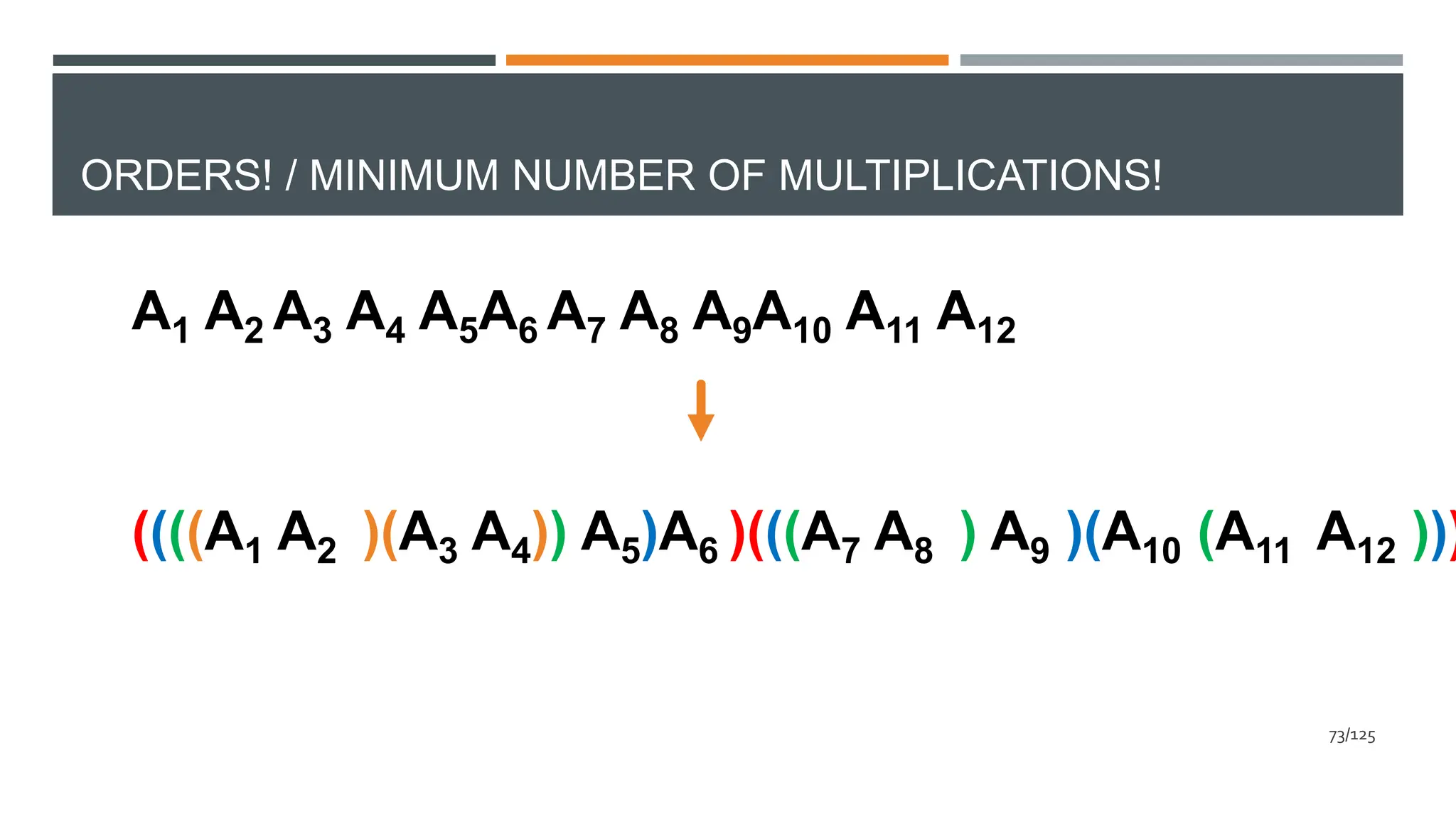
((((A1 A2 )(A3 A4)) A5)A6 )(((A7 A8 ) A9 )(A10 (A11 A12 )))
1. P[1][12]=6
1.1. P[1][6]=5
1.1.1. P[1][5]=4
1.1.1.1. P[1][4]=2
1.2. P[7][12]=9
1.2.1. P[7][9]=8
1.2.2. P[10][12]=10
92/125](https://image.slidesharecdn.com/dynamicprogramming-240626031018-00b06727/75/Data-Structures-and-algorithms-using-dynamicProgramming-92-2048.jpg)
![MATRIX CHAIN MULTIPLICATION
int MCM(int n, int d[]){
for(i=1;i<=n;i++) M[i][i]=0;// Diagonal 0
for(d=1;d<=n-1;d++) // Diagonals 1 to n-1
for(i=1;i<=n-d;i++)
{
j=i+d;
M[i][j]=Min(M[i][k]+M[k+1][j]+d[i-1]*d[k]*d[j]);
P[i][j]=min_k;
}
return M[1][n];
}
1<=k<=j-1
𝑂(𝑛3)
93/125](https://image.slidesharecdn.com/dynamicprogramming-240626031018-00b06727/75/Data-Structures-and-algorithms-using-dynamicProgramming-93-2048.jpg)
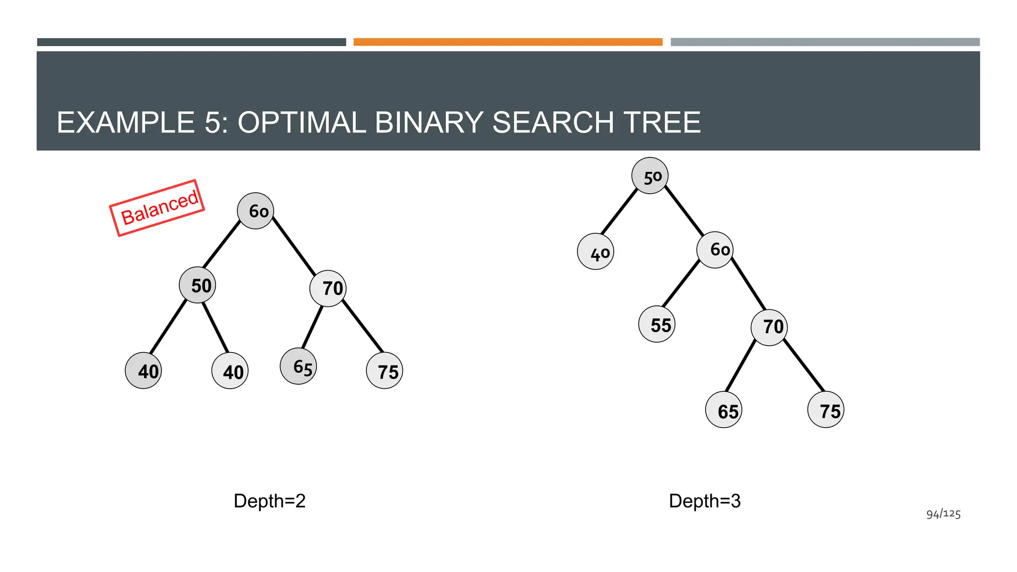
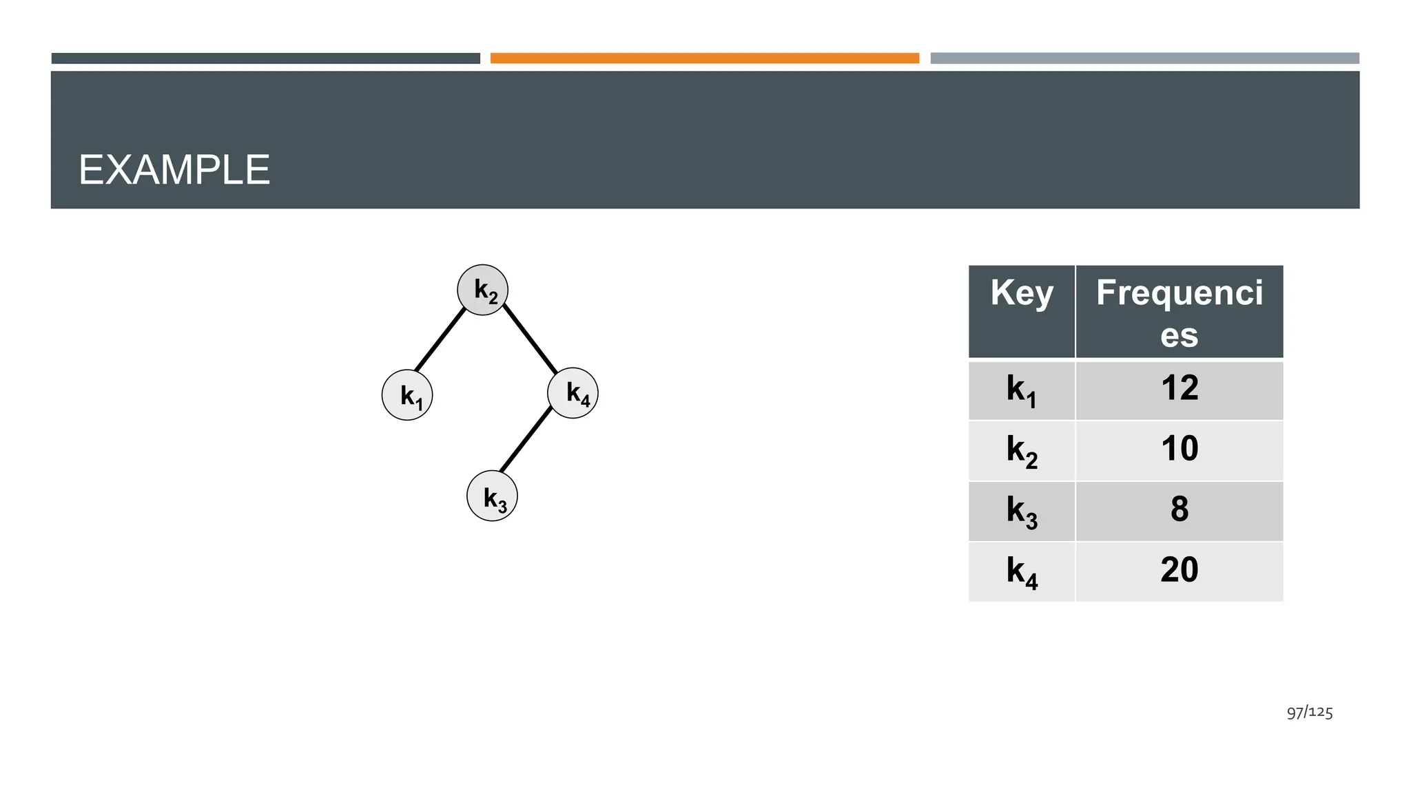
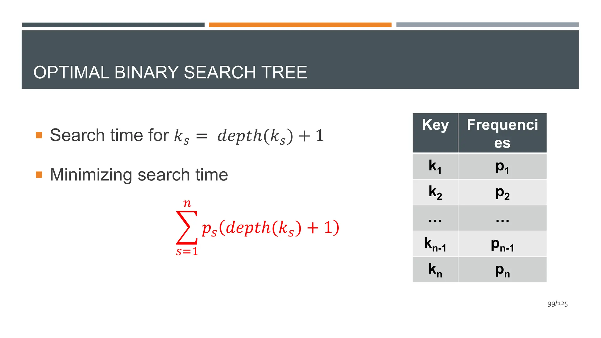
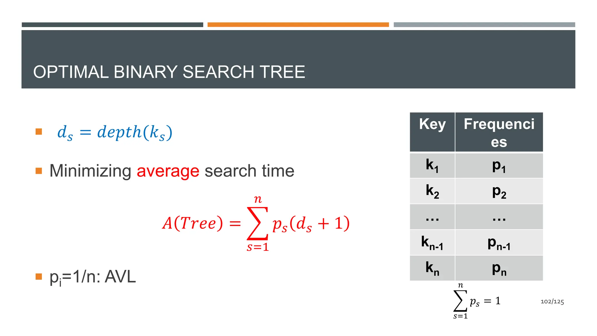
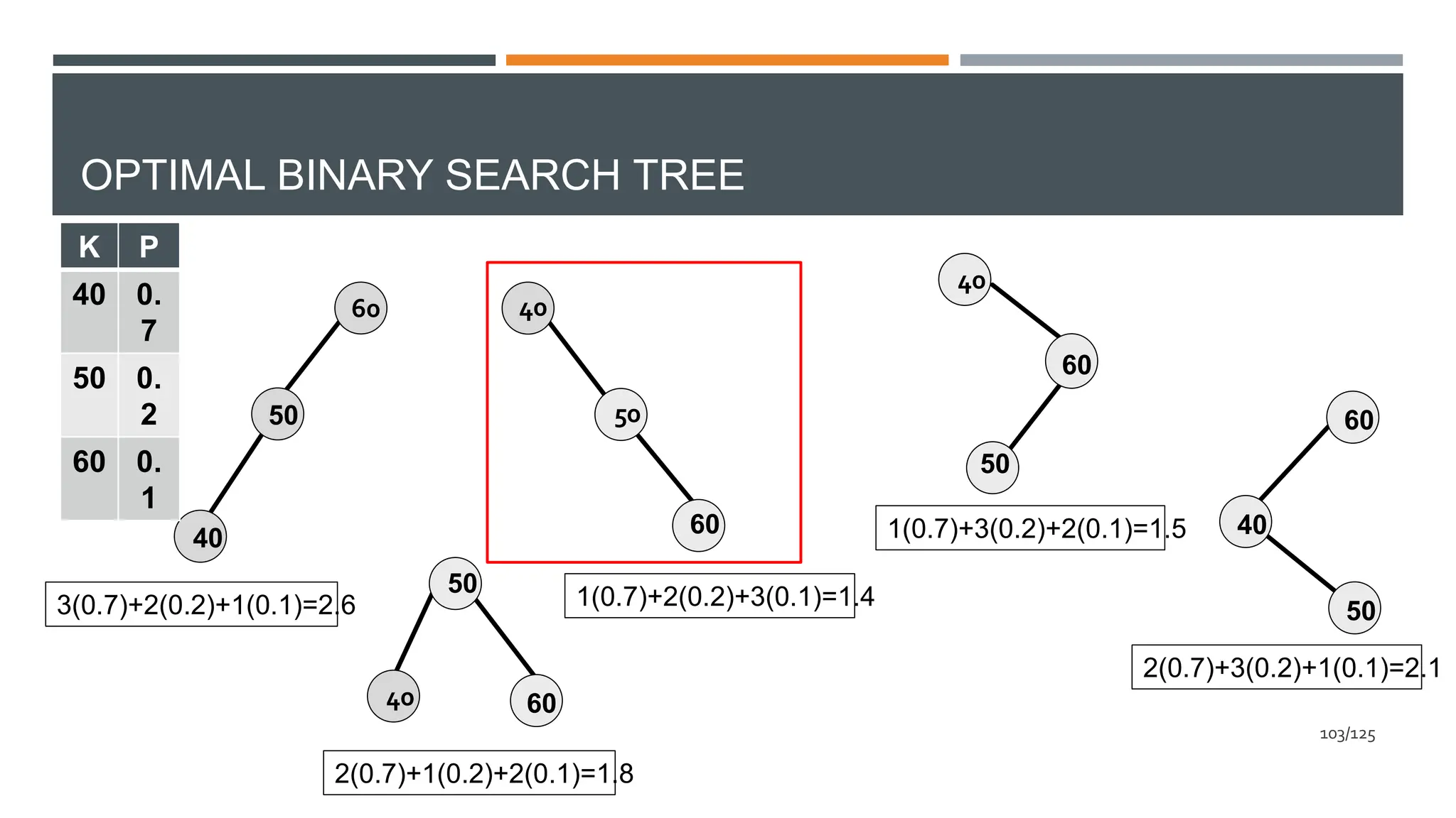
![OPTIMAL BINARY SEARCH TREE
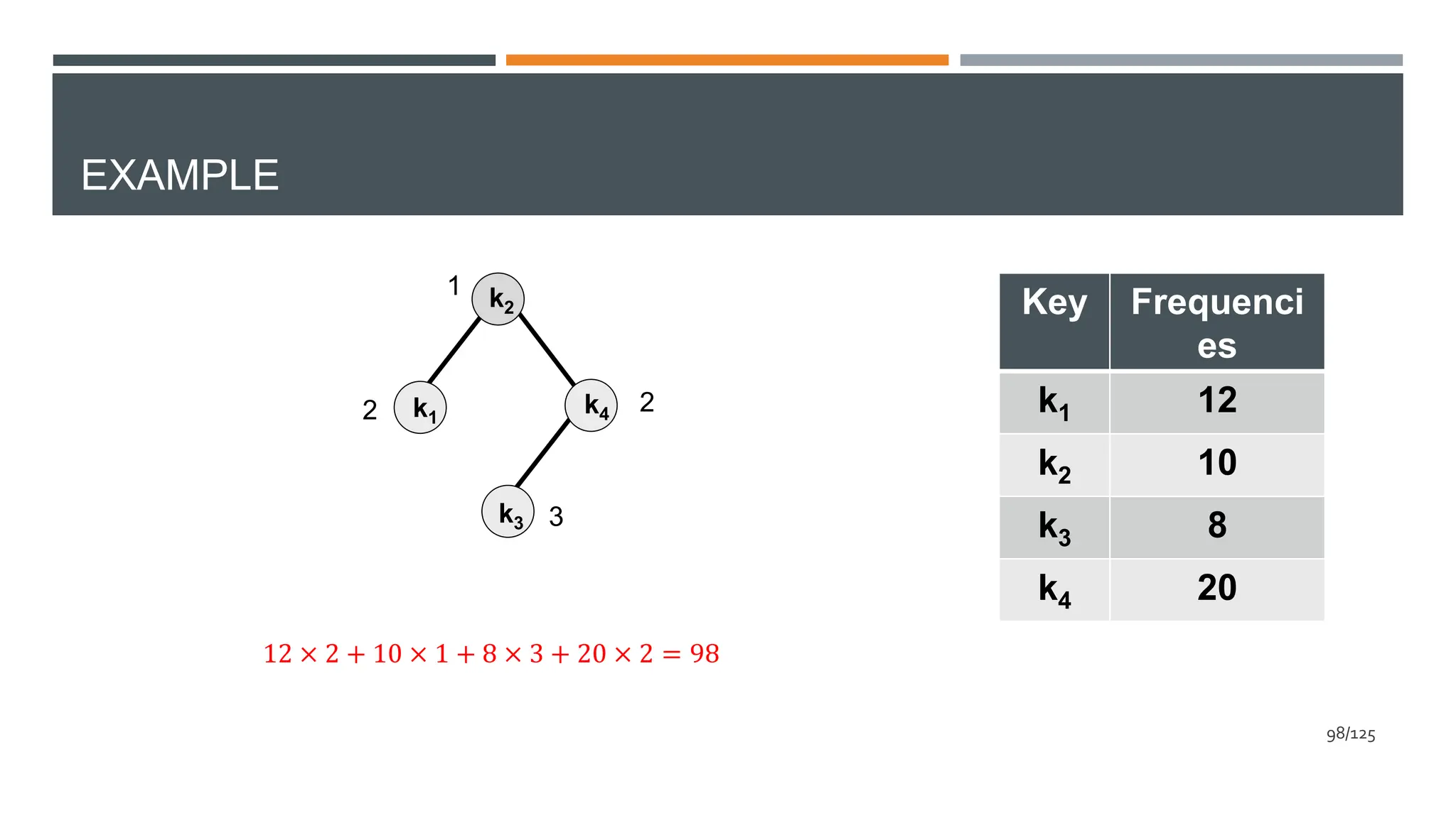
Given a sorted array key 𝑘1 ≤ 𝑘2 ≤ ⋯ ≤ 𝑘𝑛−1 ≤ 𝑘𝑛
of search keys and an array P[0.. n-1], where P[i] is
the number of searches for 𝑘𝑖.
Construct a binary search tree of all keys such that
the total cost of all the searches is as small as
possible.
Key Frequenci
es
k1 p1
k2 p2
… …
kn-1 pn-1
kn pn
96/125](https://image.slidesharecdn.com/dynamicprogramming-240626031018-00b06727/75/Data-Structures-and-algorithms-using-dynamicProgramming-96-2048.jpg)


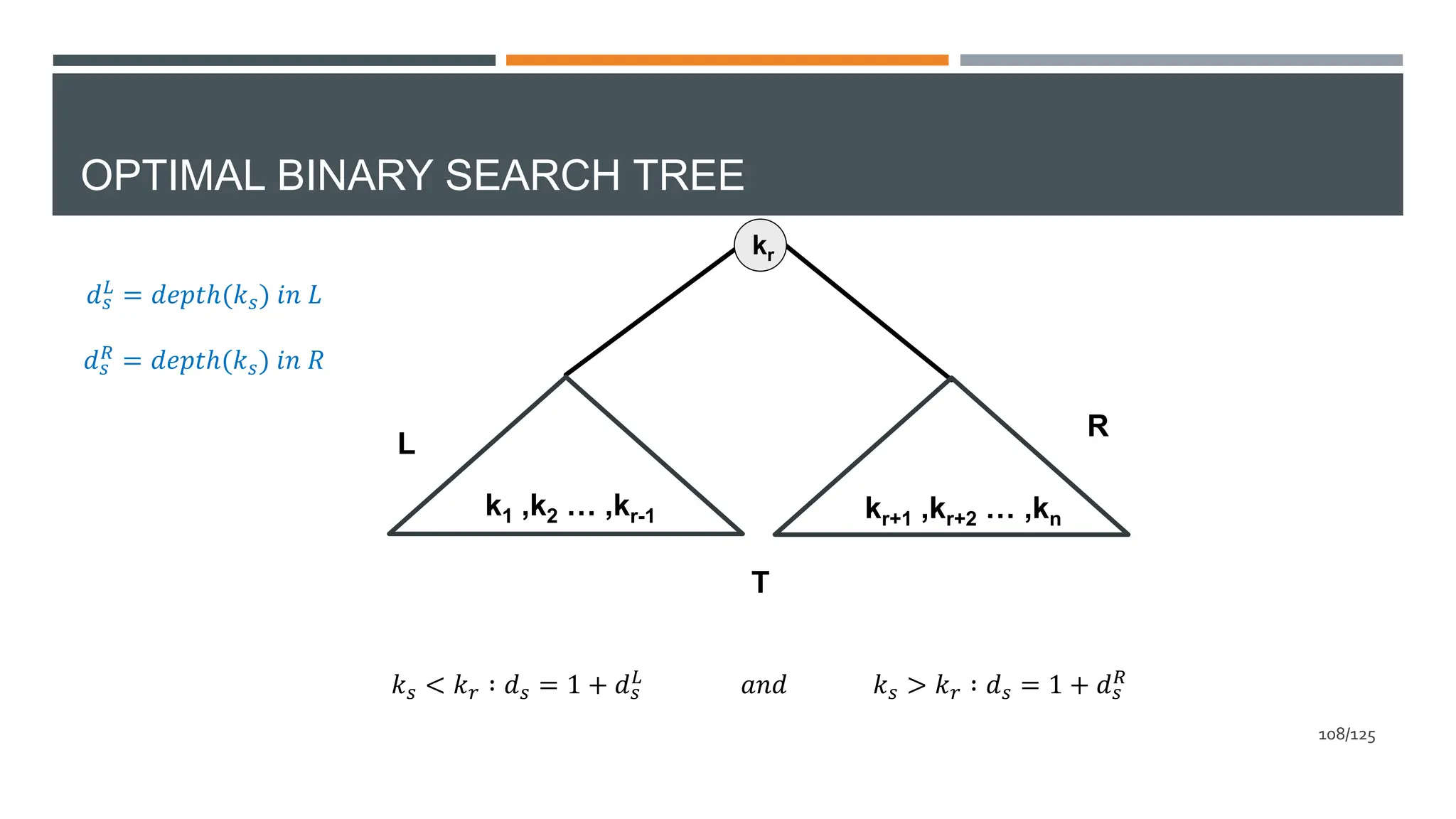
![OPTIMAL BINARY SEARCH TREE
kr
ki ,k2 … ,kr-1 kr+1 ,kr+2 … ,kj
L
R
A[i][j]=Minimum Average Search Time for a binary tree
of keys: ki, ki+1, …,kj-1, kj : 1<= i <= j <=n
104/125](https://image.slidesharecdn.com/dynamicprogramming-240626031018-00b06727/75/Data-Structures-and-algorithms-using-dynamicProgramming-104-2048.jpg)
![OPTIMAL BINARY SEARCH TREE
ki
A[i][i]=pi
105/125](https://image.slidesharecdn.com/dynamicprogramming-240626031018-00b06727/75/Data-Structures-and-algorithms-using-dynamicProgramming-105-2048.jpg)
![OPTIMAL BINARY SEARCH TREE
kr
k1 ,k2 … ,kr-1 kr+1 ,kr+2 … ,kn
L
A[1][n]=?
R
106/125](https://image.slidesharecdn.com/dynamicprogramming-240626031018-00b06727/75/Data-Structures-and-algorithms-using-dynamicProgramming-106-2048.jpg)
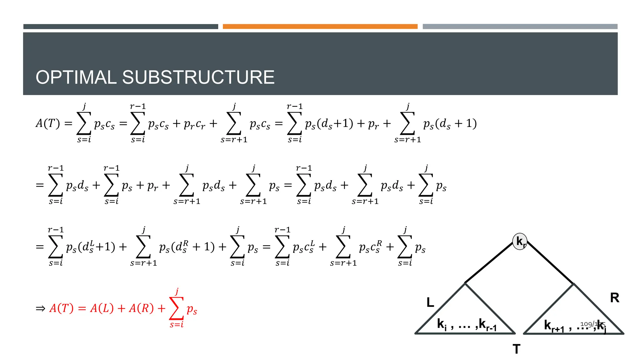
![OPTIMAL SUBSTRUCTURE
ki , … ,kr-1 kr+1 , … ,kj
L R
kr
T*
if 𝒌𝒓 is the root of optimal tree: 𝑨 𝒊 [𝒋] = 𝑨[𝒊][𝒓 − 𝟏] + 𝑨[𝒓 + 𝟏][𝒋] +
𝒔=𝒊
𝒋
𝒑𝒔
107/125](https://image.slidesharecdn.com/dynamicprogramming-240626031018-00b06727/75/Data-Structures-and-algorithms-using-dynamicProgramming-107-2048.jpg)
![CALCULATING A[I][J]
kr
ki
kj
ki+1
ki
kj-1
kj
… …
𝑨[𝒊 + 𝟏][𝒋] +
𝒔=𝒊
𝒋
𝒑𝒔 𝑨 𝒊 𝒊 + 𝑨[𝒊 + 𝟐][𝒋] +
𝒔=𝒊
𝒋
𝒑𝒔 𝑨[𝒊][𝒓 − 𝟏] + 𝑨[𝒓 + 𝟏][𝒋] +
𝒔=𝒊
𝒋
𝒑𝒔
𝑨[𝒊][𝒋 − 𝟏] +
𝒔=𝒊
𝒋
𝒑𝒔
𝑨 𝒊 𝒋 − 𝟐 + 𝑨[𝒋][𝒋] +
𝒔=𝒊
𝒋
𝒑𝒔
𝑨 𝒊 [𝒋] = 𝑴𝑰𝑵{ 𝑨[𝒊][𝒓 − 𝟏] + 𝑨[𝒓 + 𝟏][𝒋] +
𝒔=𝒊
𝒋
𝒑𝒔}
𝒊 ≤ 𝒓 ≤ 𝒋
110/125](https://image.slidesharecdn.com/dynamicprogramming-240626031018-00b06727/75/Data-Structures-and-algorithms-using-dynamicProgramming-110-2048.jpg)
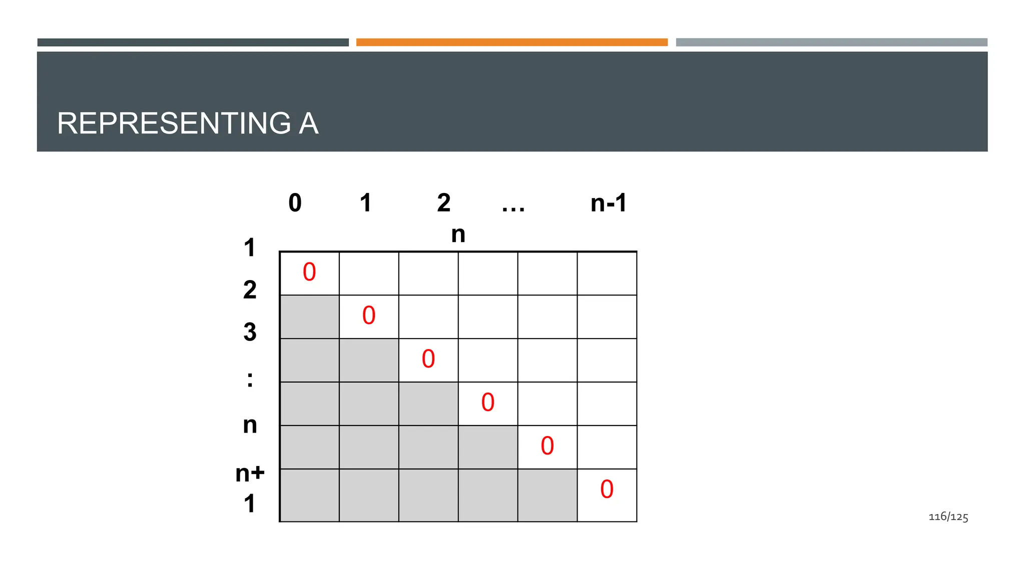
![REPRESENTING A
1
2
3
:
n
n+
1
0 1 2 … n-1
n
𝟏 ≤ 𝒊 ≤ 𝒋 ≤ 𝒏: 𝑨 𝒊 [𝒋] = 𝑴𝑰𝑵{ 𝑨[𝒊][𝒓 − 𝟏] + 𝑨[𝒓 + 𝟏][𝒋] +
𝒔=𝒊
𝒋
𝒑𝒔}
𝒊 ≤ 𝒓 ≤ 𝒋
111/125](https://image.slidesharecdn.com/dynamicprogramming-240626031018-00b06727/75/Data-Structures-and-algorithms-using-dynamicProgramming-111-2048.jpg)
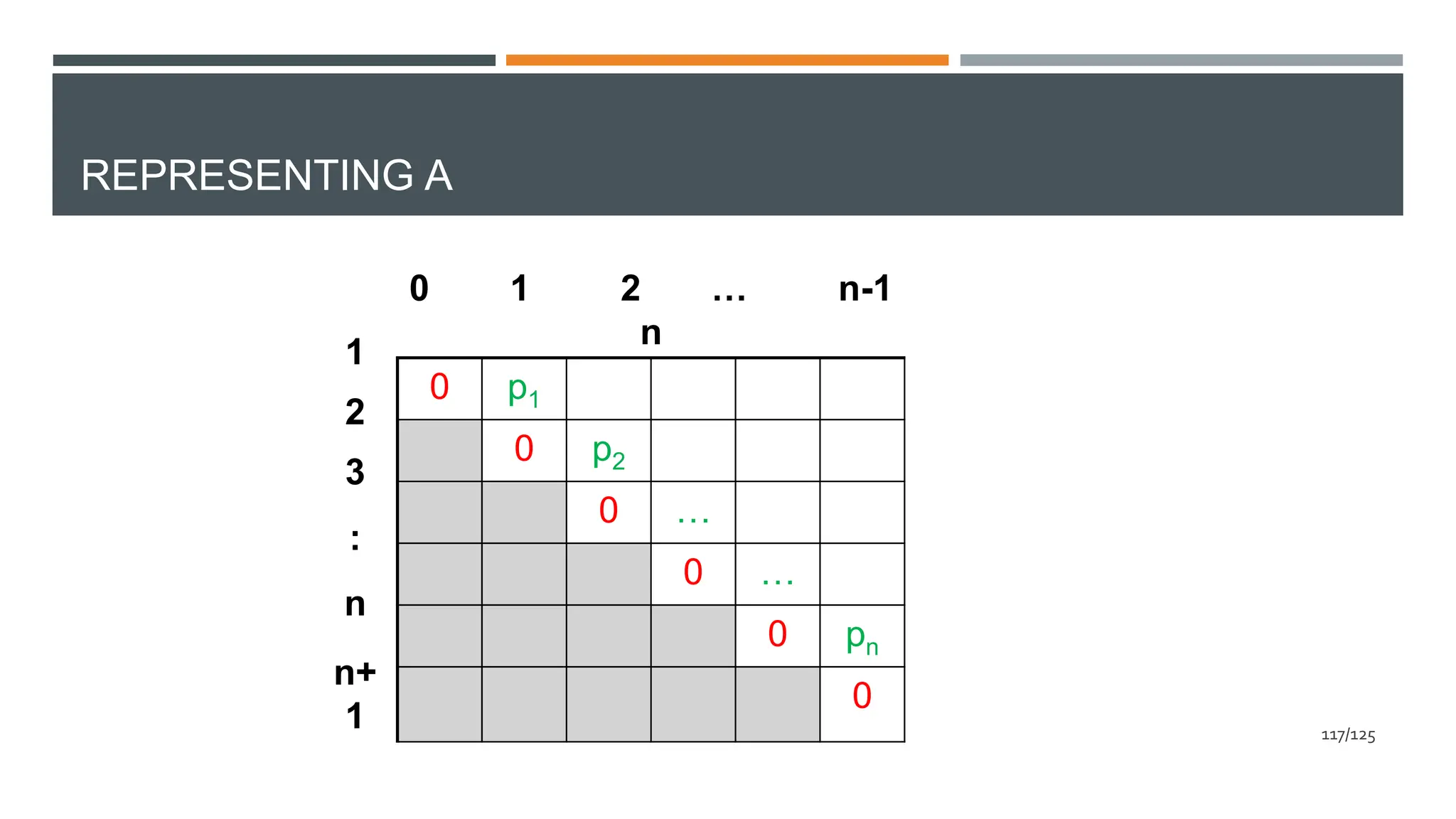
![REPRESENTING A
1
2
3
:
n
n+
1
0 1 2 … n-1
n
𝟏 ≤ 𝒊 ≤ 𝒋 ≤ 𝒏: 𝑨 𝒊 [𝒋] = 𝑴𝑰𝑵{ 𝑨[𝒊][𝒓 − 𝟏] + 𝑨[𝒓 + 𝟏][𝒋] +
𝒔=𝒊
𝒋
𝒑𝒔}
𝒊 ≤ 𝒓 ≤ 𝒋
𝒊 = 𝟏 → 𝒓 − 𝟏 = 𝟎
112/125](https://image.slidesharecdn.com/dynamicprogramming-240626031018-00b06727/75/Data-Structures-and-algorithms-using-dynamicProgramming-112-2048.jpg)
![REPRESENTING A
1
2
3
:
n
n+
1
0 1 2 … n-1
n
𝟏 ≤ 𝒊 ≤ 𝒋 ≤ 𝒏: 𝑨 𝒊 [𝒋] = 𝑴𝑰𝑵{ 𝑨[𝒊][𝒓 − 𝟏] + 𝑨[𝒓 + 𝟏][𝒋] +
𝒔=𝒊
𝒋
𝒑𝒔}
𝒊 ≤ 𝒓 ≤ 𝒋
𝒋 = 𝒏 → 𝒓 + 𝟏 = 𝒏 + 𝟏
113/125
𝒊 = 𝟏 → 𝒓 − 𝟏 = 𝟎](https://image.slidesharecdn.com/dynamicprogramming-240626031018-00b06727/75/Data-Structures-and-algorithms-using-dynamicProgramming-113-2048.jpg)
![REPRESENTING A
1
2
3
:
n
n+
1
0 1 2 … n-1
n
Diagonal 0
Diagonal 1
Diagonal d
Diagonal n-2
Diagonal n-1
Diagonal -1
A[i][i-1]: n+1
A[i][i]: n
A[i][i+1]: n-1
A[i][i+d]: n-d
A[i][i+n-2]: 2
A[1][1+n-1]: 1
Diagonal d: A[i][i+d], 1<=i<=n-d A[i][j] lies on Diagonal j-i
114/125](https://image.slidesharecdn.com/dynamicprogramming-240626031018-00b06727/75/Data-Structures-and-algorithms-using-dynamicProgramming-114-2048.jpg)
![REPRESENTING A
𝟏 ≤ 𝒊 ≤ 𝒋 ≤ 𝒏: 𝑨 𝒊 [𝒋] = 𝑴𝑰𝑵{ 𝑨[𝒊][𝒓 − 𝟏] + 𝑨[𝒓 + 𝟏][𝒋] +
𝒔=𝒊
𝒋
𝒑𝒔}
𝒊 ≤ 𝒓 ≤ 𝒋
𝒓 − 𝟏 − 𝒊 ≤ 𝒋 − 𝒊 − 𝟏 𝒋 − 𝒓 − 𝟏 ≤ 𝒋 − 𝒊 − 𝟏
𝑶𝒏 𝒅𝒊𝒂𝒈𝒐𝒏𝒂𝒍 𝒋 − 𝒊
115/125](https://image.slidesharecdn.com/dynamicprogramming-240626031018-00b06727/75/Data-Structures-and-algorithms-using-dynamicProgramming-115-2048.jpg)


![OPTIMAL BINARY SEARCH TREE
int OBST(int n, int P[]){
for(i=1;i<=n+1;i++) A[i][i-1]=0;// Diagonal -1
for(i=1;i<=n;i++) A[i][i]=P[i];// Diagonal 0
for(d=1;d<=n-1;d++) // Diagonals 1 to n-1
for(i=1;i<=n-d;i++)
{
j=i+d;
A[i][j]=Min(A[i][r-1]+A[r+1][j]+P[i]+…+P[j]);
}
return A[1][n];
}
1<=r<=j
𝑂(𝑛3)
118/125](https://image.slidesharecdn.com/dynamicprogramming-240626031018-00b06727/75/Data-Structures-and-algorithms-using-dynamicProgramming-118-2048.jpg)
![CONSTRUCTING OPTIMAL TREE
R[i][j]=r: kr is the root in the optimal Tree of ki … kj
R[i][i-1]=0, R[i][i]=i
119/125](https://image.slidesharecdn.com/dynamicprogramming-240626031018-00b06727/75/Data-Structures-and-algorithms-using-dynamicProgramming-119-2048.jpg)
![CONSTRUCTING OPTIMAL TREE
R[i][j]=r: kr is the root in the optimal Tree of ki … kj
R[i][i]=i
P
1
2
3
4
5
6
0 1 2 3
4
5
1 1 1 1 4
2 3 4 5
3 4 5
4 5
5 120/125](https://image.slidesharecdn.com/dynamicprogramming-240626031018-00b06727/75/Data-Structures-and-algorithms-using-dynamicProgramming-120-2048.jpg)
![CONSTRUCTING OPTIMAL TREE
R[i][j]=r: kr is the root in the optimal Tree of ki … kj
R[i][i-1]=0, R[i][i]=i
P
1
2
3
4
5
6
0 1 2 3
4
5
1 1 1 1 4
2 3 4 5
3 4 5
4 5
5
R[1][5]=4
k4
k1 … k3 k5
121/125](https://image.slidesharecdn.com/dynamicprogramming-240626031018-00b06727/75/Data-Structures-and-algorithms-using-dynamicProgramming-121-2048.jpg)
![CONSTRUCTING OPTIMAL TREE
R[i][j]=r: kr is the root in the optimal Tree of ki … kj
R[i][i-1]=0, R[i][i]=i
P
1
2
3
4
5
6
0 1 2 3
4
5
1 1 1 1 4
2 3 4 5
3 4 5
4 5
5
R[1][3]=1
k4
k2 , k3
k5
k1
122/125](https://image.slidesharecdn.com/dynamicprogramming-240626031018-00b06727/75/Data-Structures-and-algorithms-using-dynamicProgramming-122-2048.jpg)
![CONSTRUCTING OPTIMAL TREE
R[i][j]=r: kr is the root in the optimal Tree of ki … kj
R[i][i-1]=0, R[i][i]=i
P
1
2
3
4
5
6
0 1 2 3
4
5
1 1 1 1 4
2 3 4 5
3 4 5
4 5
5
R[2][3]=3
k4
k5
k1
k3
k2
123/125](https://image.slidesharecdn.com/dynamicprogramming-240626031018-00b06727/75/Data-Structures-and-algorithms-using-dynamicProgramming-123-2048.jpg)
![OPTIMAL BINARY SEARCH TREE
int OBST(int n, int P[]){
for(i=1;i<=n+1;i++) {A[i][i-1]=0;R[i][i-1]=0;}// Diagonal -1
for(i=1;i<=n;i++) {A[i][i]=P[i];R[i][i]=i;}// Diagonal 0
for(d=1;d<=n-1;d++) // Diagonals 1 to n-1
for(i=1;i<=n-d;i++)
{
j=i+d;
A[i][j]=Min(A[i][r-1]+A[r+1][j]+P[i]+…+P[j]);
R[i][j]=min_r;
}
return A[1][n];
}
1<=r<=j
𝑂(𝑛3)
124/125](https://image.slidesharecdn.com/dynamicprogramming-240626031018-00b06727/75/Data-Structures-and-algorithms-using-dynamicProgramming-124-2048.jpg)


![FIBONACCI’S SERIES: DP APPROACH
fib(int n)
{
F[0]=F[1]=1;
for(i=2;i<=n;i++)
F[i]=F[i-1]+F[i-2];
}
1 - - - - -
1
F
1 2 - - - -
1
F
1 2 3 - - -
1
F
1 2 3 5 - -
1
F
fib(5)=?
- - - - - -
-
F
𝑂(𝑛)
7/125](https://crownmelresort.com/image.slidesharecdn.com/dynamicprogramming-240626031018-00b06727/75/Data-Structures-and-algorithms-using-dynamicProgramming-7-2048.jpg)


![EXAMPLE 2: BINOMIAL COEFFICIENT
int BC(int n, int r)
{
for(i=0;i<=n;i++)
for(j=0;j<=r;j++)
if(i>=j)
{
if(j==0 || i==j) M[i][j]=1;
else
M[i][j]=M[i-1][j]+M[i-1][j-1];
}
return M[n][r];
}
0
1
2
3
4
0 1 2 3
4
1
1 1
1 1
1 1
1 1
14/125
𝑀 𝑖 𝑗 =
𝑖
𝑗
, 𝑗 ≤ 𝑖](https://crownmelresort.com/image.slidesharecdn.com/dynamicprogramming-240626031018-00b06727/75/Data-Structures-and-algorithms-using-dynamicProgramming-14-2048.jpg)
![EXAMPLE 2: BINOMIAL COEFFICIENT
int BC(int n, int r)
{
for(i=0;i<=n;i++)
for(j=0;j<=r;j++)
if(i>=j)
{
if(j==0 || i==j) M[i][j]=1;
else
M[i][j]=M[i-1][j]+M[i-1][j-1];
}
return M[n][r];
}
0
1
2
3
4
0 1 2 3
4
1
1 1
1 1
1 1
1 1
M[4][2]=? 15/125
𝑀 𝑖 𝑗 =
𝑖
𝑗
, 𝑗 ≤ 𝑖](https://crownmelresort.com/image.slidesharecdn.com/dynamicprogramming-240626031018-00b06727/75/Data-Structures-and-algorithms-using-dynamicProgramming-15-2048.jpg)
![EXAMPLE 2: BINOMIAL COEFFICIENT
0
1
2
3
4
0 1 2 3
4
1
1 1
1 1
1 1
1 1
M[2][1]=?
16/125](https://crownmelresort.com/image.slidesharecdn.com/dynamicprogramming-240626031018-00b06727/75/Data-Structures-and-algorithms-using-dynamicProgramming-16-2048.jpg)
![EXAMPLE 2: BINOMIAL COEFFICIENT
0
1
2
3
4
0 1 2 3
4
1
1 1
1 2 1
1 1
1 1
M[2][1]=?
17/125](https://crownmelresort.com/image.slidesharecdn.com/dynamicprogramming-240626031018-00b06727/75/Data-Structures-and-algorithms-using-dynamicProgramming-17-2048.jpg)
![EXAMPLE 2: BINOMIAL COEFFICIENT
0
1
2
3
4
0 1 2 3
4
1
1 1
1 2 1
1 1
1 1
M[3][1]=?
18/125](https://crownmelresort.com/image.slidesharecdn.com/dynamicprogramming-240626031018-00b06727/75/Data-Structures-and-algorithms-using-dynamicProgramming-18-2048.jpg)
![EXAMPLE 2: BINOMIAL COEFFICIENT
0
1
2
3
4
0 1 2 3
4
1
1 1
1 2 1
1 3 1
1 1
M[3][1]=?
19/125](https://crownmelresort.com/image.slidesharecdn.com/dynamicprogramming-240626031018-00b06727/75/Data-Structures-and-algorithms-using-dynamicProgramming-19-2048.jpg)
![EXAMPLE 2: BINOMIAL COEFFICIENT
0
1
2
3
4
0 1 2 3
4
1
1 1
1 2 1
1 3 1
1 1
M[3][2]=?
20/125](https://crownmelresort.com/image.slidesharecdn.com/dynamicprogramming-240626031018-00b06727/75/Data-Structures-and-algorithms-using-dynamicProgramming-20-2048.jpg)
![EXAMPLE 2: BINOMIAL COEFFICIENT
0
1
2
3
4
0 1 2 3
4
1
1 1
1 2 1
1 3 3 1
1 1
M[3][2]=?
21/125](https://crownmelresort.com/image.slidesharecdn.com/dynamicprogramming-240626031018-00b06727/75/Data-Structures-and-algorithms-using-dynamicProgramming-21-2048.jpg)
![EXAMPLE 2: BINOMIAL COEFFICIENT
0
1
2
3
4
0 1 2 3
4
1
1 1
1 2 1
1 3 3 1
1 1
M[4][1]=?
22/125](https://crownmelresort.com/image.slidesharecdn.com/dynamicprogramming-240626031018-00b06727/75/Data-Structures-and-algorithms-using-dynamicProgramming-22-2048.jpg)
![EXAMPLE 2: BINOMIAL COEFFICIENT
0
1
2
3
4
0 1 2 3
4
1
1 1
1 2 1
1 3 3 1
1 4 1
M[4][1]=?
23/125](https://crownmelresort.com/image.slidesharecdn.com/dynamicprogramming-240626031018-00b06727/75/Data-Structures-and-algorithms-using-dynamicProgramming-23-2048.jpg)
![EXAMPLE 2: BINOMIAL COEFFICIENT
0
1
2
3
4
0 1 2 3
4
1
1 1
1 2 1
1 3 3 1
1 4 1
M[4][2]=?
24/125](https://crownmelresort.com/image.slidesharecdn.com/dynamicprogramming-240626031018-00b06727/75/Data-Structures-and-algorithms-using-dynamicProgramming-24-2048.jpg)
![EXAMPLE 2: BINOMIAL COEFFICIENT
0
1
2
3
4
0 1 2 3
4
1
1 1
1 2 1
1 3 3 1
1 4 6 1
M[4][2]=?
25/125](https://crownmelresort.com/image.slidesharecdn.com/dynamicprogramming-240626031018-00b06727/75/Data-Structures-and-algorithms-using-dynamicProgramming-25-2048.jpg)
![BINOMIAL COEFFICIENT: TIME COMPLEXITY
int BC(int n, int r)
{
for(i=0;i<=n;i++)
for(j=0;j<=r;j++)
if(i>=j)
{
if(j==0 || i==j) M[i][j]=1;
else
M[i][j]=M[i-1][j]+M[i-1][j-1];
}
return M[n][r];
}
26/125
𝑂(𝑛𝑟)](https://crownmelresort.com/image.slidesharecdn.com/dynamicprogramming-240626031018-00b06727/75/Data-Structures-and-algorithms-using-dynamicProgramming-26-2048.jpg)


![GRAPH: REPRESENTATION
A D
C
E
G
B
1
1
5
9
3
2 4 2
3
3
A B C D E
A 0 1
8
1 5
B 9 0 3 2
8
C
8
8
0 4
8
D
8
8
2 0 3
E 3
8
8
8
0
W
31/125
W[i][j]=weight of edge from vertex i to j](https://crownmelresort.com/image.slidesharecdn.com/dynamicprogramming-240626031018-00b06727/75/Data-Structures-and-algorithms-using-dynamicProgramming-31-2048.jpg)
![SHORTEST PATHS: REPRESENTATION
A D
C
E
G
B
1
1
5
9
3
2 4 2
3
3
A B C D E
A 0 1 3 1 4
B 8 0 3 2 5
C 10 11 0 4 7
D 6 7 2 0 3
E 3 4 6 4 0
D
32/125
D[i][j]=length of shortest path from vertex i to j](https://crownmelresort.com/image.slidesharecdn.com/dynamicprogramming-240626031018-00b06727/75/Data-Structures-and-algorithms-using-dynamicProgramming-32-2048.jpg)


![SUBPROBLEMS: REPRESENTATION
v1 v4
v3
v5
v2
1
1
5
9
3
2 4 2
3
3
v1 v2 v3 v4 v5
v1 0 1 4 1 5
v2 9 0 3 2 14
v3 ∞ ∞ 0 4 ∞
v4 ∞ ∞ 2 0 3
v5 3 4 7 4 0
D
(3)
D [i][j]=length of shortest path between vi and vj in
the graph restricted to vertices {v1,v2,…,vk}
(k)
46/125](https://crownmelresort.com/image.slidesharecdn.com/dynamicprogramming-240626031018-00b06727/75/Data-Structures-and-algorithms-using-dynamicProgramming-46-2048.jpg)

![CALCULATING DS
vi vj
D [i][j]
(k+1)
48/125](https://crownmelresort.com/image.slidesharecdn.com/dynamicprogramming-240626031018-00b06727/75/Data-Structures-and-algorithms-using-dynamicProgramming-48-2048.jpg)
![CALCULATING DS
vi vj
D [i][j]
(k+1)
vi vj
vi vj
Vk+1
49/125](https://crownmelresort.com/image.slidesharecdn.com/dynamicprogramming-240626031018-00b06727/75/Data-Structures-and-algorithms-using-dynamicProgramming-49-2048.jpg)
![CALCULATING DS
vi vj
D [i][j]
(k+1)
vi vj
vi vj
Vk+1
D(k)[i][j]
D [i][k+1]+D [k+1][j]
(k) (k)
D [i][k+1]+D [k+1][j],
(k) (k)
D [i][j]=min{
(k+1)
D [i][j]}
(k) 50/125](https://crownmelresort.com/image.slidesharecdn.com/dynamicprogramming-240626031018-00b06727/75/Data-Structures-and-algorithms-using-dynamicProgramming-50-2048.jpg)


![FLOYD’S METHOD: ALGORITHM
Floyd(int W[][], int n)
{
D=W;//initializing D0
for(k=1;k<=n;k++) //calculating Dk
for(i=1;i<=n;i++)
for(j=1;j<=n;j++)
D[i][j]=min{D[i][j],D[i][k]+D[k][j]};
return D;
}
𝑂(𝑛3
)
55/125](https://crownmelresort.com/image.slidesharecdn.com/dynamicprogramming-240626031018-00b06727/75/Data-Structures-and-algorithms-using-dynamicProgramming-55-2048.jpg)
![FLOYD’S METHOD: ALGORITHM
Floyd(int W[][], int n)
{
D=W;//initializing D0
for(k=1;k<=n;k++) //calculating Dk
for(i=1;i<=n;i++)
for(j=1;j<=n;j++)
if(D[i][k]+D[k][j]<D[i][j])
D[i][j]=D[i][k]+D[k][j];
return D;
}
𝑂(𝑛3
)
56/125](https://crownmelresort.com/image.slidesharecdn.com/dynamicprogramming-240626031018-00b06727/75/Data-Structures-and-algorithms-using-dynamicProgramming-56-2048.jpg)
![SHORTEST PATHS!
Rows and columns of P: v1 to vn
P[i][j]=r: shortest path from vi to vj passes through vr
P[i][j]=0: edge vivj is the shortest path from vi to vj
1. How can I calculate P?
2. How can I use P for finding shortest paths?
57/125](https://crownmelresort.com/image.slidesharecdn.com/dynamicprogramming-240626031018-00b06727/75/Data-Structures-and-algorithms-using-dynamicProgramming-57-2048.jpg)
![SHORTEST PATHS!
P[i][j]=r: shortest path from vi to vj passes through vr
P[i][j]=0: edge vivj is the shortest path from vi to vj
v1 v2 v3 v4
v1 0 0 4 2
v2 4 0 4 0
v3 0 1 0 0
v4 0 1 0 0
P
58/125](https://crownmelresort.com/image.slidesharecdn.com/dynamicprogramming-240626031018-00b06727/75/Data-Structures-and-algorithms-using-dynamicProgramming-58-2048.jpg)
![SHORTEST PATHS!
v1 v2 v3 v4
v1 0 0 4 2
v2 4 0 4 0
v3 0 1 0 0
v4 0 1 0 0
P
SP(v1,v3)=?? v1 v3
59/125
P[i][j]=r: shortest path from vi to vj passes through vr
P[i][j]=0: edge vivj is the shortest path from vi to vj](https://crownmelresort.com/image.slidesharecdn.com/dynamicprogramming-240626031018-00b06727/75/Data-Structures-and-algorithms-using-dynamicProgramming-59-2048.jpg)
![SHORTEST PATHS!
v1 v2 v3 v4
v1 0 0 4 2
v2 4 0 4 0
v3 0 1 0 0
v4 0 1 0 0
P
SP(v1,v3)=??
P[v1][v3]=4
v1 v3
v4
60/125
P[i][j]=r: shortest path from vi to vj passes through vr
P[i][j]=0: edge vivj is the shortest path from vi to vj](https://crownmelresort.com/image.slidesharecdn.com/dynamicprogramming-240626031018-00b06727/75/Data-Structures-and-algorithms-using-dynamicProgramming-60-2048.jpg)
![SHORTEST PATHS!
v1 v2 v3 v4
v1 0 0 4 2
v2 4 0 4 0
v3 0 1 0 0
v4 0 1 0 0
P
SP(v1,v3)=??
P[v1][v3]=4
1. SP(v1,v4)=?
2. SP(v4,v3)=?
v1 v3
v4
61/125
P[i][j]=r: shortest path from vi to vj passes through vr
P[i][j]=0: edge vivj is the shortest path from vi to vj](https://crownmelresort.com/image.slidesharecdn.com/dynamicprogramming-240626031018-00b06727/75/Data-Structures-and-algorithms-using-dynamicProgramming-61-2048.jpg)
![SHORTEST PATHS!
v1 v2 v3 v4
v1 0 0 4 2
v2 4 0 4 0
v3 0 1 0 0
v4 0 1 0 0
P
SP(v1,v3)=??
P[v1][v3]=4
1. P[v1][v4]=?
2. P[v4][v3]=?
v1 v3
v4
62/125
P[i][j]=r: shortest path from vi to vj passes through vr
P[i][j]=0: edge vivj is the shortest path from vi to vj](https://crownmelresort.com/image.slidesharecdn.com/dynamicprogramming-240626031018-00b06727/75/Data-Structures-and-algorithms-using-dynamicProgramming-62-2048.jpg)
![SHORTEST PATHS!
v1 v2 v3 v4
v1 0 0 4 2
v2 4 0 4 0
v3 0 1 0 0
v4 0 1 0 0
P
SP(v1,v3)=??
P[v1][v3]=4
1. P[v1][v4]=2
2. P[v4][v3]=0
v1 v3
v4
63/125
P[i][j]=r: shortest path from vi to vj passes through vr
P[i][j]=0: edge vivj is the shortest path from vi to vj](https://crownmelresort.com/image.slidesharecdn.com/dynamicprogramming-240626031018-00b06727/75/Data-Structures-and-algorithms-using-dynamicProgramming-63-2048.jpg)
![SHORTEST PATHS!
v1 v2 v3 v4
v1 0 0 4 2
v2 4 0 4 0
v3 0 1 0 0
v4 0 1 0 0
P
SP(v1,v3)=??
P[v1][v3]=4
1. P[v1][v4]=2
2. P[v4][v3]=0
v1
v2
64/125
v4
v3
P[i][j]=r: shortest path from vi to vj passes through vr
P[i][j]=0: edge vivj is the shortest path from vi to vj](https://crownmelresort.com/image.slidesharecdn.com/dynamicprogramming-240626031018-00b06727/75/Data-Structures-and-algorithms-using-dynamicProgramming-64-2048.jpg)
![SHORTEST PATHS!
v1 v2 v3 v4
v1 0 0 4 2
v2 4 0 4 0
v3 0 1 0 0
v4 0 1 0 0
P
SP(v1,v3)=??
P[v1][v3]=4
1. P[v1][v4]=2
1.1. P[v1][v2]=0
1.2. P[v2][v4]=0
2. P[v4][v3]=0
v1
v2
65/125
v3
v4
P[i][j]=r: shortest path from vi to vj passes through vr
P[i][j]=0: edge vivj is the shortest path from vi to vj](https://crownmelresort.com/image.slidesharecdn.com/dynamicprogramming-240626031018-00b06727/75/Data-Structures-and-algorithms-using-dynamicProgramming-65-2048.jpg)
![SHORTEST PATHS!
v1 v2 v3 v4
v1 0 0 4 2
v2 4 0 4 0
v3 0 1 0 0
v4 0 1 0 0
P
SP(v1,v3)=??
P[v1][v3]=4
1. P[v1][v4]=2
1.1. P[v1][v2]=0
1.2. P[v2][v4]=0
2. P[v4][v3]=0
v2
66/125
v3
v4
v1
P[i][j]=r: shortest path from vi to vj passes through vr
P[i][j]=0: edge vivj is the shortest path from vi to vj](https://crownmelresort.com/image.slidesharecdn.com/dynamicprogramming-240626031018-00b06727/75/Data-Structures-and-algorithms-using-dynamicProgramming-66-2048.jpg)
![CALCULATING P
vi vj
D [i][j]
(k+1)
vi vj
vi vj
Vk+1
P[i][j]=k+1
D [i][k+1]+D [k+1][j] : P[i][j]=k+1
(k) (k)
If D [i][j]=
(k+1) 67/125](https://crownmelresort.com/image.slidesharecdn.com/dynamicprogramming-240626031018-00b06727/75/Data-Structures-and-algorithms-using-dynamicProgramming-67-2048.jpg)
![FLOYD’S ALGORITHM
Floyd(int W[][], int n){
D=W;
P=0;
for(k=1;k<=n;k++)
for(i=1;i<=n;i++)
for(j=1;j<=n;j++)
if(D[i][k]+D[k][j]<D[i][j])
{
D[i][j]=D[i][k]+D[k][j];
P[i][j]=k+1;
}
return D;
}
68/125](https://crownmelresort.com/image.slidesharecdn.com/dynamicprogramming-240626031018-00b06727/75/Data-Structures-and-algorithms-using-dynamicProgramming-68-2048.jpg)


![DEFINING SUBPROBLEMS
Find the most efficient way to multiply the following matrices
together:
For i>=j, M[i][j]=0
M[1][n]=Optimum number of multiplications.
A x A x … x A
i i+1 j
M[i][j]=Minimum number of multiplications
in product Ai Ai+1 … Aj , i<j
74/125](https://crownmelresort.com/image.slidesharecdn.com/dynamicprogramming-240626031018-00b06727/75/Data-Structures-and-algorithms-using-dynamicProgramming-74-2048.jpg)
![CALCULATING M[I][J] A A … A
i i+1 j
d d
j
di-1 i
M[i+1][j]+
d d
j
di-1 i+1
M[i][i+1]+M[i+2][j]+
d d
j
di-1 i+2
M[i][i+2]+M[i+3][j]+
d d
j
di-1 k
M[i][k]+M[k+1][j]+
…
…
d d
j
di-1 j-3
M[i][j-3]+M[j-2][j]+
d d
j
di-1 j-2
M[i][j-2]+M[j-1][j]+
d d
j
di-1 j-1
M[i][j-1]+
(A … A )(A … A )
i i+2 i+3 j
(A … A )(A … A )
i j-3 j-2 j
(A A )(A … A )
i i+1 i+2 j
A (A … A )
i i+1 j
…
(A … A )(A … A )
i k k+1 j
…
(A … A )(A A )
i j-2 j-1 j
(A … A ) A
i j-1 j
MIN
75/125](https://crownmelresort.com/image.slidesharecdn.com/dynamicprogramming-240626031018-00b06727/75/Data-Structures-and-algorithms-using-dynamicProgramming-75-2048.jpg)
![CALCULATING M[I][J]
A A … A
i i+1 j
(A … A )(A … A )
i k k+1 j
d d
j
di-1 k
M[i][j]= MIN { M[i][k]+M[k+1][j] + }
i<=k<j
MIN
M[i][i]= 0 76/125](https://crownmelresort.com/image.slidesharecdn.com/dynamicprogramming-240626031018-00b06727/75/Data-Structures-and-algorithms-using-dynamicProgramming-76-2048.jpg)
![CALCULATING M
1
2
3
4
:
n
1 2 3 4
…
n
M[i][j]=?
A A … A
i i+1 j
77/125](https://crownmelresort.com/image.slidesharecdn.com/dynamicprogramming-240626031018-00b06727/75/Data-Structures-and-algorithms-using-dynamicProgramming-77-2048.jpg)
![CALCULATING M
M[i][j]=?
A A … A
i i+1 j
i<=j 1
2
3
4
:
n
1 2 3 4
…
n
78/125](https://crownmelresort.com/image.slidesharecdn.com/dynamicprogramming-240626031018-00b06727/75/Data-Structures-and-algorithms-using-dynamicProgramming-78-2048.jpg)
![CALCULATING M
Diagonal 0
Diagonal 1
Diagonal 2
Diagonal n-2
Diagonal n-1
M[i][i]: n
M[i][i+1]: n-1
M[i][i+2]: n-2
M[i][i+d]: n-d
M[i][i+n-2]: 2
M[1][1+n-1]: 1
Diagonal d: M[i][i+d], 1<=i<=n-d M[i][j] lies on Diagonal j-i
1
2
3
4
:
n
1 2 3 4
…
n
Diagonal d
79/125](https://crownmelresort.com/image.slidesharecdn.com/dynamicprogramming-240626031018-00b06727/75/Data-Structures-and-algorithms-using-dynamicProgramming-79-2048.jpg)
![CALCULATING M
M[i][i]=0
1
2
3
4
:
n
1 2 3 4
…
n
0
0
0
0
0
0
80/125](https://crownmelresort.com/image.slidesharecdn.com/dynamicprogramming-240626031018-00b06727/75/Data-Structures-and-algorithms-using-dynamicProgramming-80-2048.jpg)
![CALCULATING M
d d
i+1
di-1 k
M[i][i+1]= MIN { M[i][k]+M[k+1][i+1]+ }=
i<=k<i+1
d d
i+1
di-1 i
M[i][i]+M[i+1][i+1]+ i+1
=d d d
i-1 i
d d
2
d0 1
1
2
3
4
:
n
1 2 3 4
…
n
0
0
0
0
0
0
81/125](https://crownmelresort.com/image.slidesharecdn.com/dynamicprogramming-240626031018-00b06727/75/Data-Structures-and-algorithms-using-dynamicProgramming-81-2048.jpg)
![CALCULATING M
d di+2
di-1 k
M[i][i+2]= MIN { M[i][k]+M[k+1][i+2]+ }=
i<=k<i+2
d di+2
di-1 i
MIN{M[i][i]+M[i+1][i+2]+ d di+2
di-1 i+1
, M[i][i+1]+M[i+2][i+2]+ }
1
2
3
4
:
n
1 2 3 4 … n
0
0
0
0
0
0
82/125](https://crownmelresort.com/image.slidesharecdn.com/dynamicprogramming-240626031018-00b06727/75/Data-Structures-and-algorithms-using-dynamicProgramming-82-2048.jpg)
![CALCULATING M
d dj
di-1 k
M[i][j]= MIN { M[i][k]+M[k+1][j] + }
i<=k<j
k-i<j-i j-k-1<j-i
1
2
3
4
:
n
1 2 3 4 … n
83/125
Diagonal j-i](https://crownmelresort.com/image.slidesharecdn.com/dynamicprogramming-240626031018-00b06727/75/Data-Structures-and-algorithms-using-dynamicProgramming-83-2048.jpg)
![MATRIX CHAIN MULTIPLICATION
int MCM(int n, int d[]){
for(i=1;i<=n;i++) M[i][i]=0;// Diagonal 0
for(d=1;d<=n-1;d++) // Diagonals 1 to n-1
for(i=1;i<=n-d;i++)
{
j=i+d;
M[i][j]=Min(M[i][k]+M[k+1][j]+d[i-1]*d[k]*d[j]);
}
return M[1][n];
}
i<=k<=j-1
𝑂(𝑛3)
84/125](https://crownmelresort.com/image.slidesharecdn.com/dynamicprogramming-240626031018-00b06727/75/Data-Structures-and-algorithms-using-dynamicProgramming-84-2048.jpg)
![ORDERS!
P[i][j]=k: the optimal order is
(A … A )(A … A )
i k k+1 j
85/125](https://crownmelresort.com/image.slidesharecdn.com/dynamicprogramming-240626031018-00b06727/75/Data-Structures-and-algorithms-using-dynamicProgramming-85-2048.jpg)
![ORDERS!
P[i][j]=k: the optimal order is
P[i][i+1]=i
(A … A )(A … A )
i k k+1 j
86/125](https://crownmelresort.com/image.slidesharecdn.com/dynamicprogramming-240626031018-00b06727/75/Data-Structures-and-algorithms-using-dynamicProgramming-86-2048.jpg)
![ORDERS!
P
A1 A2 A3 A4 A5 A6
P[i][j]=k: the optimal order is
P[i][i+1]=i
(A … A )(A … A )
i k k+1 j
1
2
3
4
5
6
1 2 3 4
5
6
1 1 1 1
3 4 5
4 5
5
87/125](https://crownmelresort.com/image.slidesharecdn.com/dynamicprogramming-240626031018-00b06727/75/Data-Structures-and-algorithms-using-dynamicProgramming-87-2048.jpg)
![ORDERS!
P
A1 A2 A3 A4 A5 A6
P[1][6]=1
P[i][j]=k: the optimal order is
(A … A )(A … A )
i k k+1 j
1
2
3
4
5
6
1 2 3 4
5
6
1 1 1 1
3 4 5
4 5
5
A1 (A2 A3 A4 A5 A6)
88/125](https://crownmelresort.com/image.slidesharecdn.com/dynamicprogramming-240626031018-00b06727/75/Data-Structures-and-algorithms-using-dynamicProgramming-88-2048.jpg)
![ORDERS!
P
A1 A2 A3 A4 A5 A6
P[1][6]=1
P[2][6]=5
P[i][j]=k: the optimal order is
P[i][i+1]=i
(A … A )(A … A )
i k k+1 j
1
2
3
4
5
6
1 2 3 4
5
6
1 1 1 1
3 4 5
4 5
5
A1 (A2 A3 A4 A5 A6)
A1 ((A2 A3 A4 A5 ) A6)
89/125](https://crownmelresort.com/image.slidesharecdn.com/dynamicprogramming-240626031018-00b06727/75/Data-Structures-and-algorithms-using-dynamicProgramming-89-2048.jpg)
![ORDERS!
P
A1 A2 A3 A4 A5 A6
P[1][6]=1
P[2][6]=5
P[2][5]=4
P[i][j]=k: the optimal order is
P[i][i+1]=i
(A … A )(A … A )
i k k+1 j
1
2
3
4
5
6
1 2 3 4
5
6
1 1 1 1
3 4 5
4 5
5
A1 (A2 A3 A4 A5 A6)
A1 ((A2 A3 A4 A5 ) A6)
A1 (((A2 A3 A4 )A5 ) A6)
90/125](https://crownmelresort.com/image.slidesharecdn.com/dynamicprogramming-240626031018-00b06727/75/Data-Structures-and-algorithms-using-dynamicProgramming-90-2048.jpg)
![ORDERS!
P
A1 A2 A3 A4 A5 A6
P[1][6]=1
P[2][6]=5
P[2][5]=4
P[2][4]=3
P[i][j]=k: the optimal order is
j>=i+1
(A … A )(A … A )
i k k+1 j
1
2
3
4
5
6
1 2 3 4
5
6
1 1 1 3
3 4 5
4 5
5
A1 (A2 A3 A4 A5 A6)
A1 ((A2 A3 A4 A5 ) A6)
A1 (((A2 A3 A4 )A5 ) A6)
A1 ((((A2 A3 )A4 )A5 ) A6)
91/125](https://crownmelresort.com/image.slidesharecdn.com/dynamicprogramming-240626031018-00b06727/75/Data-Structures-and-algorithms-using-dynamicProgramming-91-2048.jpg)
![ORDERS!
((((A1 A2 )(A3 A4)) A5)A6 )(((A7 A8 ) A9 )(A10 (A11 A12 )))
1. P[1][12]=6
1.1. P[1][6]=5
1.1.1. P[1][5]=4
1.1.1.1. P[1][4]=2
1.2. P[7][12]=9
1.2.1. P[7][9]=8
1.2.2. P[10][12]=10
92/125](https://crownmelresort.com/image.slidesharecdn.com/dynamicprogramming-240626031018-00b06727/75/Data-Structures-and-algorithms-using-dynamicProgramming-92-2048.jpg)
![MATRIX CHAIN MULTIPLICATION
int MCM(int n, int d[]){
for(i=1;i<=n;i++) M[i][i]=0;// Diagonal 0
for(d=1;d<=n-1;d++) // Diagonals 1 to n-1
for(i=1;i<=n-d;i++)
{
j=i+d;
M[i][j]=Min(M[i][k]+M[k+1][j]+d[i-1]*d[k]*d[j]);
P[i][j]=min_k;
}
return M[1][n];
}
1<=k<=j-1
𝑂(𝑛3)
93/125](https://crownmelresort.com/image.slidesharecdn.com/dynamicprogramming-240626031018-00b06727/75/Data-Structures-and-algorithms-using-dynamicProgramming-93-2048.jpg)


![OPTIMAL BINARY SEARCH TREE
Given a sorted array key 𝑘1 ≤ 𝑘2 ≤ ⋯ ≤ 𝑘𝑛−1 ≤ 𝑘𝑛
of search keys and an array P[0.. n-1], where P[i] is
the number of searches for 𝑘𝑖.
Construct a binary search tree of all keys such that
the total cost of all the searches is as small as
possible.
Key Frequenci
es
k1 p1
k2 p2
… …
kn-1 pn-1
kn pn
96/125](https://crownmelresort.com/image.slidesharecdn.com/dynamicprogramming-240626031018-00b06727/75/Data-Structures-and-algorithms-using-dynamicProgramming-96-2048.jpg)


![OPTIMAL BINARY SEARCH TREE
kr
ki ,k2 … ,kr-1 kr+1 ,kr+2 … ,kj
L
R
A[i][j]=Minimum Average Search Time for a binary tree
of keys: ki, ki+1, …,kj-1, kj : 1<= i <= j <=n
104/125](https://crownmelresort.com/image.slidesharecdn.com/dynamicprogramming-240626031018-00b06727/75/Data-Structures-and-algorithms-using-dynamicProgramming-104-2048.jpg)
![OPTIMAL BINARY SEARCH TREE
ki
A[i][i]=pi
105/125](https://crownmelresort.com/image.slidesharecdn.com/dynamicprogramming-240626031018-00b06727/75/Data-Structures-and-algorithms-using-dynamicProgramming-105-2048.jpg)
![OPTIMAL BINARY SEARCH TREE
kr
k1 ,k2 … ,kr-1 kr+1 ,kr+2 … ,kn
L
A[1][n]=?
R
106/125](https://crownmelresort.com/image.slidesharecdn.com/dynamicprogramming-240626031018-00b06727/75/Data-Structures-and-algorithms-using-dynamicProgramming-106-2048.jpg)
![OPTIMAL SUBSTRUCTURE
ki , … ,kr-1 kr+1 , … ,kj
L R
kr
T*
if 𝒌𝒓 is the root of optimal tree: 𝑨 𝒊 [𝒋] = 𝑨[𝒊][𝒓 − 𝟏] + 𝑨[𝒓 + 𝟏][𝒋] +
𝒔=𝒊
𝒋
𝒑𝒔
107/125](https://crownmelresort.com/image.slidesharecdn.com/dynamicprogramming-240626031018-00b06727/75/Data-Structures-and-algorithms-using-dynamicProgramming-107-2048.jpg)


![CALCULATING A[I][J]
kr
ki
kj
ki+1
ki
kj-1
kj
… …
𝑨[𝒊 + 𝟏][𝒋] +
𝒔=𝒊
𝒋
𝒑𝒔 𝑨 𝒊 𝒊 + 𝑨[𝒊 + 𝟐][𝒋] +
𝒔=𝒊
𝒋
𝒑𝒔 𝑨[𝒊][𝒓 − 𝟏] + 𝑨[𝒓 + 𝟏][𝒋] +
𝒔=𝒊
𝒋
𝒑𝒔
𝑨[𝒊][𝒋 − 𝟏] +
𝒔=𝒊
𝒋
𝒑𝒔
𝑨 𝒊 𝒋 − 𝟐 + 𝑨[𝒋][𝒋] +
𝒔=𝒊
𝒋
𝒑𝒔
𝑨 𝒊 [𝒋] = 𝑴𝑰𝑵{ 𝑨[𝒊][𝒓 − 𝟏] + 𝑨[𝒓 + 𝟏][𝒋] +
𝒔=𝒊
𝒋
𝒑𝒔}
𝒊 ≤ 𝒓 ≤ 𝒋
110/125](https://crownmelresort.com/image.slidesharecdn.com/dynamicprogramming-240626031018-00b06727/75/Data-Structures-and-algorithms-using-dynamicProgramming-110-2048.jpg)
![REPRESENTING A
1
2
3
:
n
n+
1
0 1 2 … n-1
n
𝟏 ≤ 𝒊 ≤ 𝒋 ≤ 𝒏: 𝑨 𝒊 [𝒋] = 𝑴𝑰𝑵{ 𝑨[𝒊][𝒓 − 𝟏] + 𝑨[𝒓 + 𝟏][𝒋] +
𝒔=𝒊
𝒋
𝒑𝒔}
𝒊 ≤ 𝒓 ≤ 𝒋
111/125](https://crownmelresort.com/image.slidesharecdn.com/dynamicprogramming-240626031018-00b06727/75/Data-Structures-and-algorithms-using-dynamicProgramming-111-2048.jpg)
![REPRESENTING A
1
2
3
:
n
n+
1
0 1 2 … n-1
n
𝟏 ≤ 𝒊 ≤ 𝒋 ≤ 𝒏: 𝑨 𝒊 [𝒋] = 𝑴𝑰𝑵{ 𝑨[𝒊][𝒓 − 𝟏] + 𝑨[𝒓 + 𝟏][𝒋] +
𝒔=𝒊
𝒋
𝒑𝒔}
𝒊 ≤ 𝒓 ≤ 𝒋
𝒊 = 𝟏 → 𝒓 − 𝟏 = 𝟎
112/125](https://crownmelresort.com/image.slidesharecdn.com/dynamicprogramming-240626031018-00b06727/75/Data-Structures-and-algorithms-using-dynamicProgramming-112-2048.jpg)
![REPRESENTING A
1
2
3
:
n
n+
1
0 1 2 … n-1
n
𝟏 ≤ 𝒊 ≤ 𝒋 ≤ 𝒏: 𝑨 𝒊 [𝒋] = 𝑴𝑰𝑵{ 𝑨[𝒊][𝒓 − 𝟏] + 𝑨[𝒓 + 𝟏][𝒋] +
𝒔=𝒊
𝒋
𝒑𝒔}
𝒊 ≤ 𝒓 ≤ 𝒋
𝒋 = 𝒏 → 𝒓 + 𝟏 = 𝒏 + 𝟏
113/125
𝒊 = 𝟏 → 𝒓 − 𝟏 = 𝟎](https://crownmelresort.com/image.slidesharecdn.com/dynamicprogramming-240626031018-00b06727/75/Data-Structures-and-algorithms-using-dynamicProgramming-113-2048.jpg)
![REPRESENTING A
1
2
3
:
n
n+
1
0 1 2 … n-1
n
Diagonal 0
Diagonal 1
Diagonal d
Diagonal n-2
Diagonal n-1
Diagonal -1
A[i][i-1]: n+1
A[i][i]: n
A[i][i+1]: n-1
A[i][i+d]: n-d
A[i][i+n-2]: 2
A[1][1+n-1]: 1
Diagonal d: A[i][i+d], 1<=i<=n-d A[i][j] lies on Diagonal j-i
114/125](https://crownmelresort.com/image.slidesharecdn.com/dynamicprogramming-240626031018-00b06727/75/Data-Structures-and-algorithms-using-dynamicProgramming-114-2048.jpg)
![REPRESENTING A
𝟏 ≤ 𝒊 ≤ 𝒋 ≤ 𝒏: 𝑨 𝒊 [𝒋] = 𝑴𝑰𝑵{ 𝑨[𝒊][𝒓 − 𝟏] + 𝑨[𝒓 + 𝟏][𝒋] +
𝒔=𝒊
𝒋
𝒑𝒔}
𝒊 ≤ 𝒓 ≤ 𝒋
𝒓 − 𝟏 − 𝒊 ≤ 𝒋 − 𝒊 − 𝟏 𝒋 − 𝒓 − 𝟏 ≤ 𝒋 − 𝒊 − 𝟏
𝑶𝒏 𝒅𝒊𝒂𝒈𝒐𝒏𝒂𝒍 𝒋 − 𝒊
115/125](https://crownmelresort.com/image.slidesharecdn.com/dynamicprogramming-240626031018-00b06727/75/Data-Structures-and-algorithms-using-dynamicProgramming-115-2048.jpg)
![OPTIMAL BINARY SEARCH TREE
int OBST(int n, int P[]){
for(i=1;i<=n+1;i++) A[i][i-1]=0;// Diagonal -1
for(i=1;i<=n;i++) A[i][i]=P[i];// Diagonal 0
for(d=1;d<=n-1;d++) // Diagonals 1 to n-1
for(i=1;i<=n-d;i++)
{
j=i+d;
A[i][j]=Min(A[i][r-1]+A[r+1][j]+P[i]+…+P[j]);
}
return A[1][n];
}
1<=r<=j
𝑂(𝑛3)
118/125](https://crownmelresort.com/image.slidesharecdn.com/dynamicprogramming-240626031018-00b06727/75/Data-Structures-and-algorithms-using-dynamicProgramming-118-2048.jpg)
![CONSTRUCTING OPTIMAL TREE
R[i][j]=r: kr is the root in the optimal Tree of ki … kj
R[i][i-1]=0, R[i][i]=i
119/125](https://crownmelresort.com/image.slidesharecdn.com/dynamicprogramming-240626031018-00b06727/75/Data-Structures-and-algorithms-using-dynamicProgramming-119-2048.jpg)
![CONSTRUCTING OPTIMAL TREE
R[i][j]=r: kr is the root in the optimal Tree of ki … kj
R[i][i]=i
P
1
2
3
4
5
6
0 1 2 3
4
5
1 1 1 1 4
2 3 4 5
3 4 5
4 5
5 120/125](https://crownmelresort.com/image.slidesharecdn.com/dynamicprogramming-240626031018-00b06727/75/Data-Structures-and-algorithms-using-dynamicProgramming-120-2048.jpg)
![CONSTRUCTING OPTIMAL TREE
R[i][j]=r: kr is the root in the optimal Tree of ki … kj
R[i][i-1]=0, R[i][i]=i
P
1
2
3
4
5
6
0 1 2 3
4
5
1 1 1 1 4
2 3 4 5
3 4 5
4 5
5
R[1][5]=4
k4
k1 … k3 k5
121/125](https://crownmelresort.com/image.slidesharecdn.com/dynamicprogramming-240626031018-00b06727/75/Data-Structures-and-algorithms-using-dynamicProgramming-121-2048.jpg)
![CONSTRUCTING OPTIMAL TREE
R[i][j]=r: kr is the root in the optimal Tree of ki … kj
R[i][i-1]=0, R[i][i]=i
P
1
2
3
4
5
6
0 1 2 3
4
5
1 1 1 1 4
2 3 4 5
3 4 5
4 5
5
R[1][3]=1
k4
k2 , k3
k5
k1
122/125](https://crownmelresort.com/image.slidesharecdn.com/dynamicprogramming-240626031018-00b06727/75/Data-Structures-and-algorithms-using-dynamicProgramming-122-2048.jpg)
![CONSTRUCTING OPTIMAL TREE
R[i][j]=r: kr is the root in the optimal Tree of ki … kj
R[i][i-1]=0, R[i][i]=i
P
1
2
3
4
5
6
0 1 2 3
4
5
1 1 1 1 4
2 3 4 5
3 4 5
4 5
5
R[2][3]=3
k4
k5
k1
k3
k2
123/125](https://crownmelresort.com/image.slidesharecdn.com/dynamicprogramming-240626031018-00b06727/75/Data-Structures-and-algorithms-using-dynamicProgramming-123-2048.jpg)
![OPTIMAL BINARY SEARCH TREE
int OBST(int n, int P[]){
for(i=1;i<=n+1;i++) {A[i][i-1]=0;R[i][i-1]=0;}// Diagonal -1
for(i=1;i<=n;i++) {A[i][i]=P[i];R[i][i]=i;}// Diagonal 0
for(d=1;d<=n-1;d++) // Diagonals 1 to n-1
for(i=1;i<=n-d;i++)
{
j=i+d;
A[i][j]=Min(A[i][r-1]+A[r+1][j]+P[i]+…+P[j]);
R[i][j]=min_r;
}
return A[1][n];
}
1<=r<=j
𝑂(𝑛3)
124/125](https://crownmelresort.com/image.slidesharecdn.com/dynamicprogramming-240626031018-00b06727/75/Data-Structures-and-algorithms-using-dynamicProgramming-124-2048.jpg)


![SHS_Core_CAE_Q3_LE1 FOR THIRD [FINAL].pdf](https://cdn.slidesharecdn.com/ss_thumbnails/shscorecaeq3le1final-251116055110-e3081055-thumbnail.jpg?width=640&height=640&fit=bounds)


