Downloaded 34 times


![Pseudocode
1. int Chain( int i, int j )
2. {
3. int min = 10000, value, k;
4. if( i == j ){
5. return 0;
6. }
7. else{
8. for( k = i; k < j; k++ ){
9. value = (Chain(i, k) + Chain(k + 1, j) + (dimensions[i-1] *
dimensions[k] * dimensions[j]));
10. if( min > value ){
11. min = value;
12. mat[i][j] = k;
13. }
14. }
15. }
16. return min;](https://image.slidesharecdn.com/presentation1-150601195355-lva1-app6892/75/dynamic-programming-complete-by-Mumtaz-Ali-03154103173-48-2048.jpg)
![1. int main(void)
2. {
3. int result, i;
4. printf("Enter number of matrices: ");
5. scanf("%d", &n);
6. printf("Enter dimensions : ");
7. for( i = 0; i <= n; i++ ){
8. scanf("%d", &dimensions[i]);
9. }
10. result = Chain(1, n);
11. printf("nTotal number of multiplications: %d andn", result);
12. printf("Multiplication order is: ");
13. PrintOrder( 1, n );
14. printf("n");
15. }](https://image.slidesharecdn.com/presentation1-150601195355-lva1-app6892/75/dynamic-programming-complete-by-Mumtaz-Ali-03154103173-49-2048.jpg)


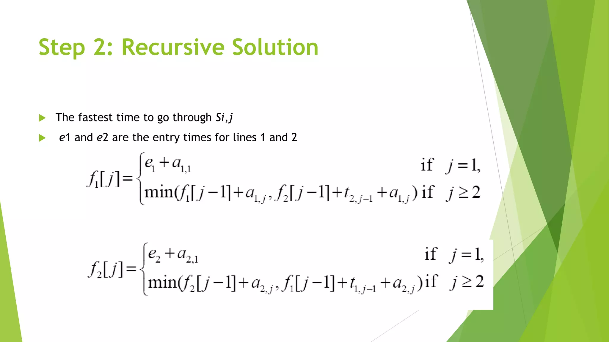
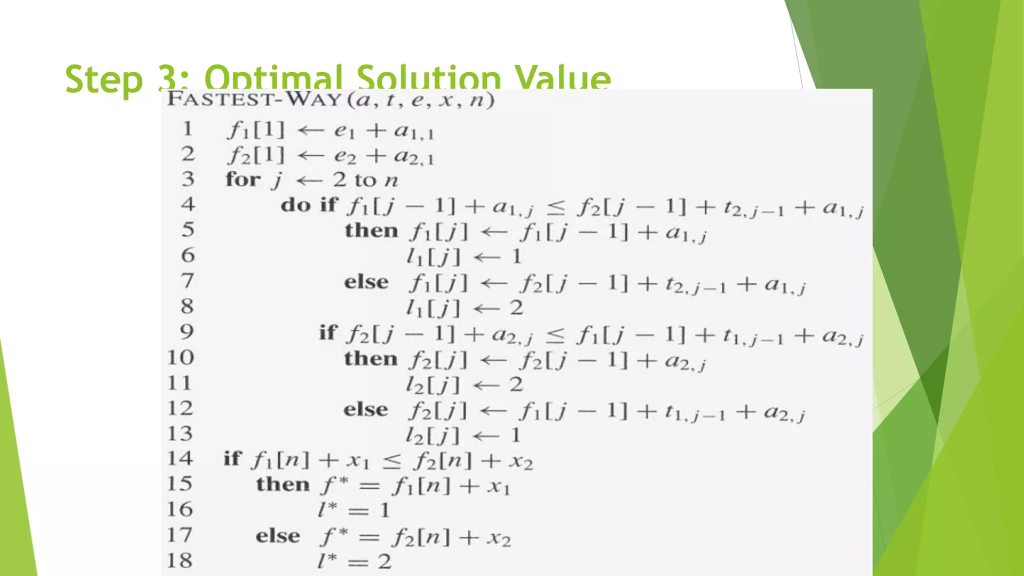
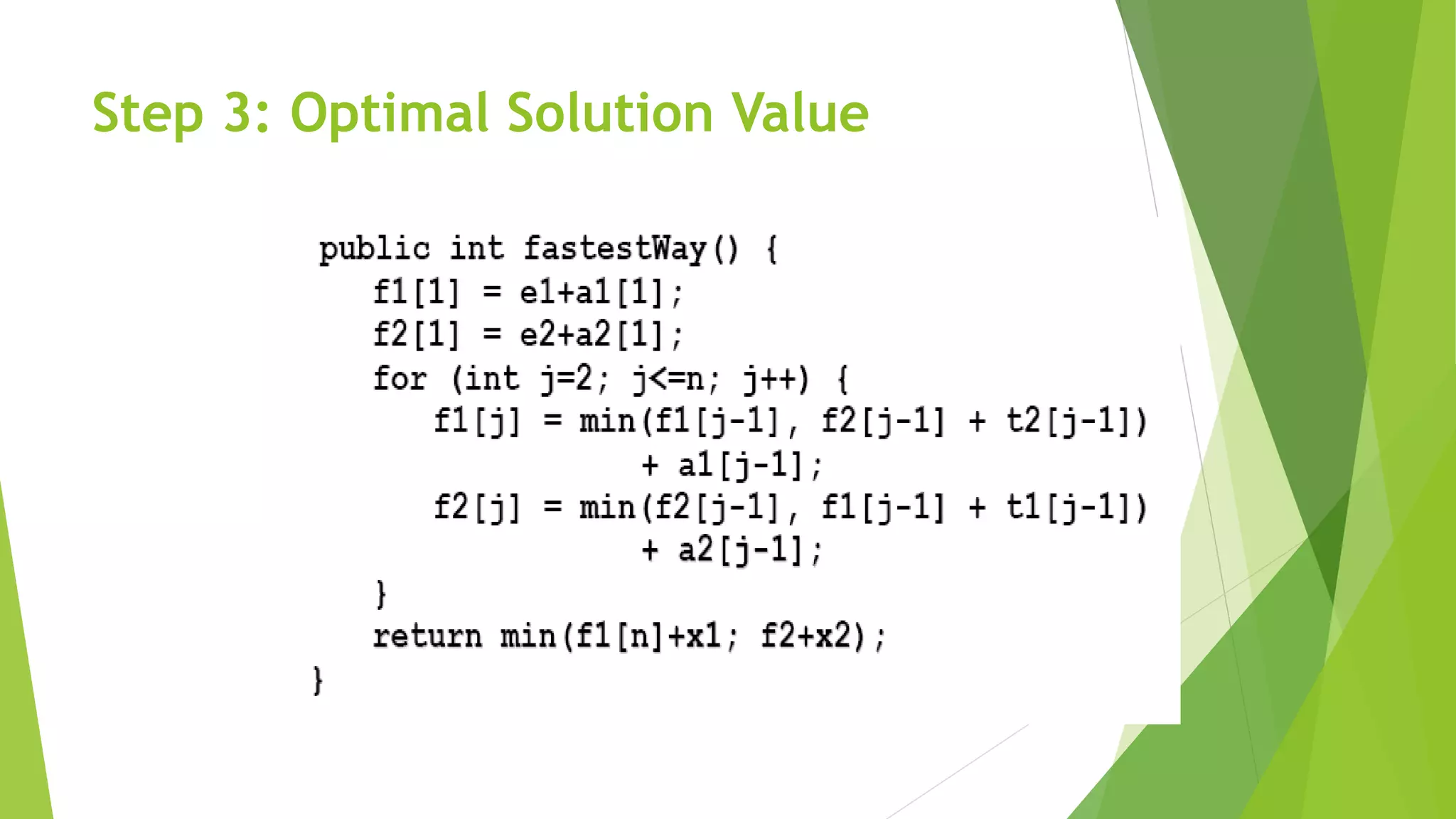
![Step 2: Recursive Solution
Define the value of an optimal solution recursively in terms of the
optimal solution to sub-problems
Sub-problem here
finding the fastest way through station j on both lines (i=1,2)
Let fi [j] be the fastest possible time to go from starting point through Si,j
The fastest time to go all the way through the factory: f*
x1 and x2 are the exit times from lines 1 and 2, respectively](https://image.slidesharecdn.com/presentation1-150601195355-lva1-app6892/75/dynamic-programming-complete-by-Mumtaz-Ali-03154103173-65-2048.jpg)
![Step 2: Recursive Solution
To help us keep track of how to construct an optimal solution, let us define
li[j ]: line # whose station j-1 is used in a fastest way through Si,j (i = 1, 2, and j =
2, 3,..., n)
we avoid defining li[1] because no station precedes station 1 on either lines.
We also define
l*: the line whose station n is used in a fastest way through the entire factory](https://image.slidesharecdn.com/presentation1-150601195355-lva1-app6892/75/dynamic-programming-complete-by-Mumtaz-Ali-03154103173-69-2048.jpg)
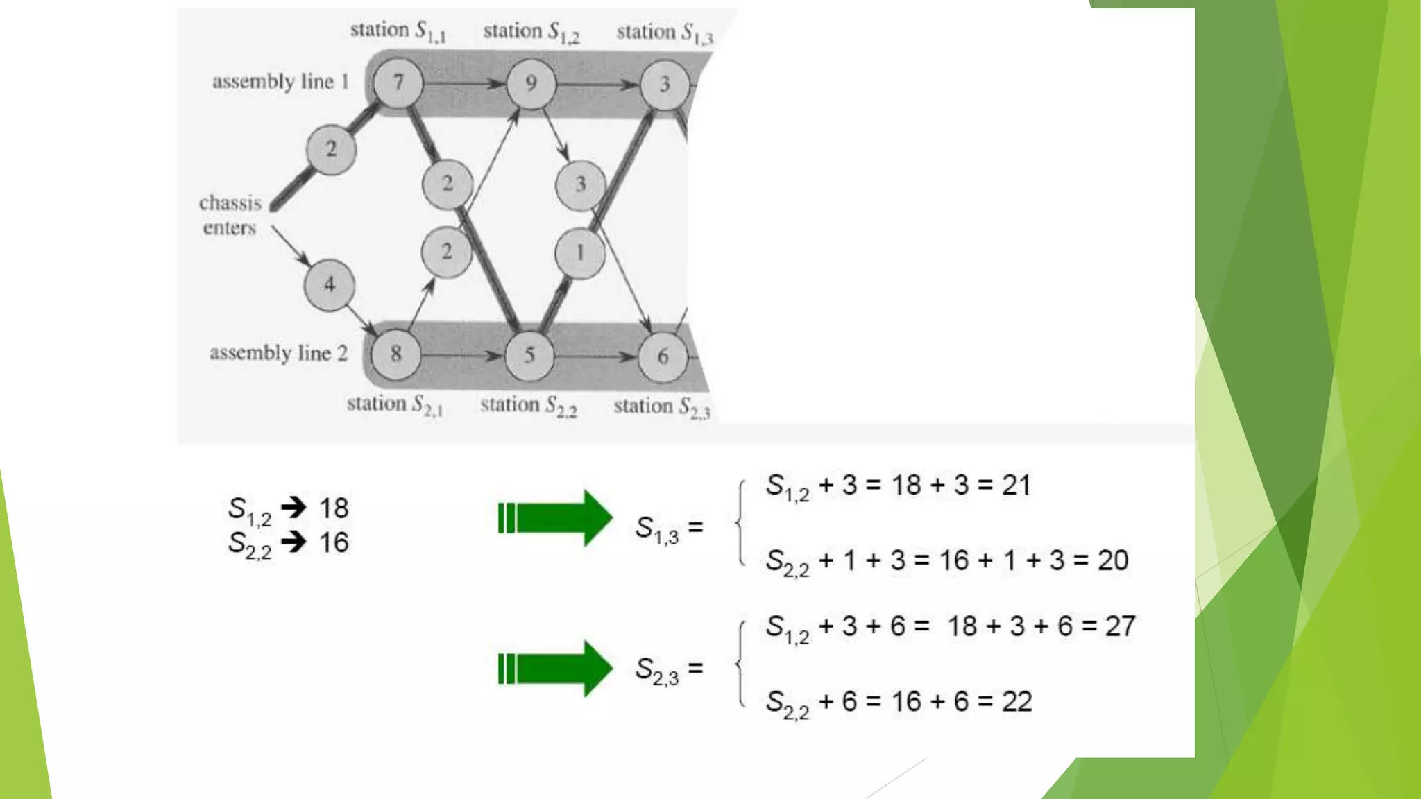
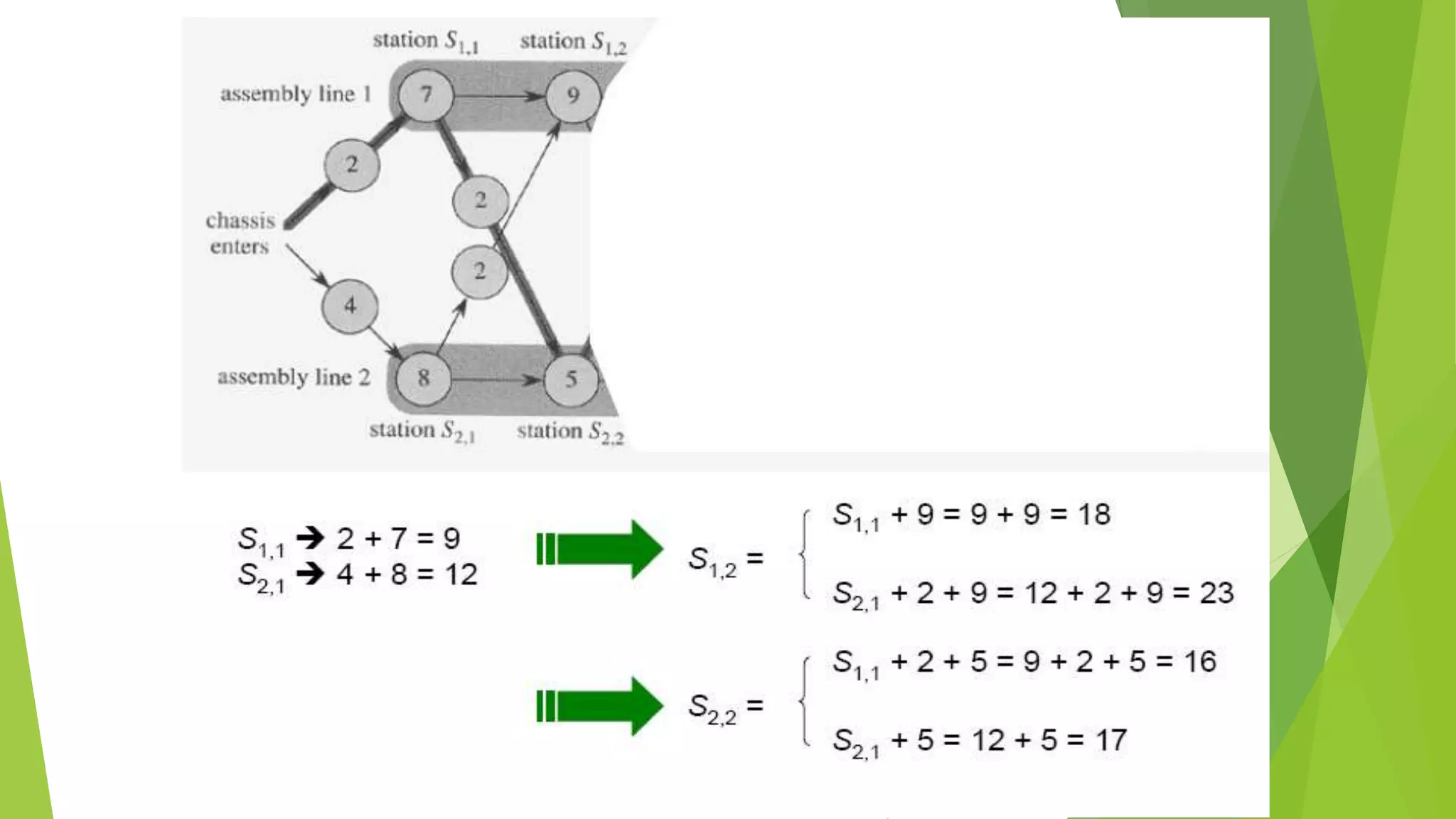
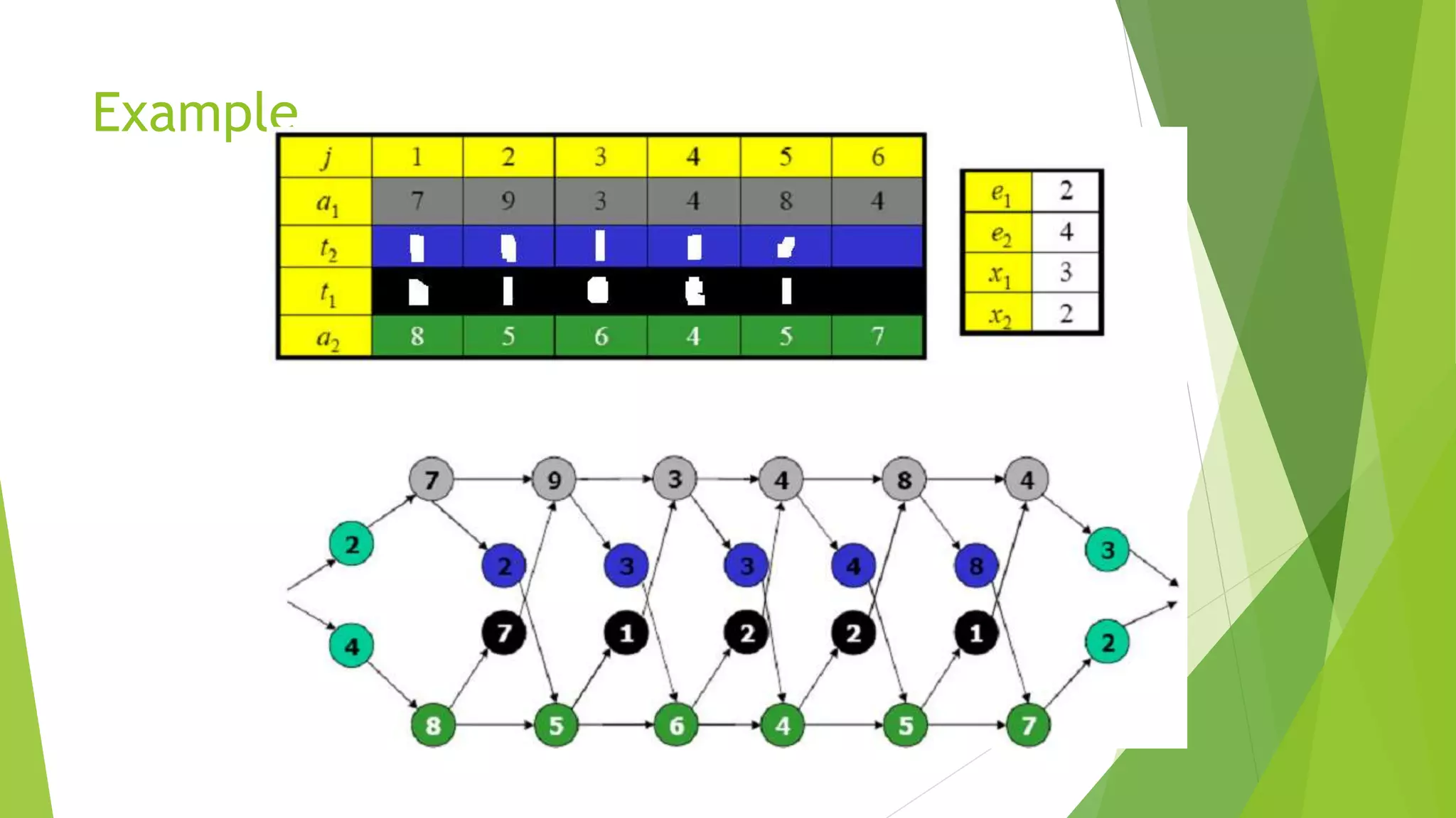
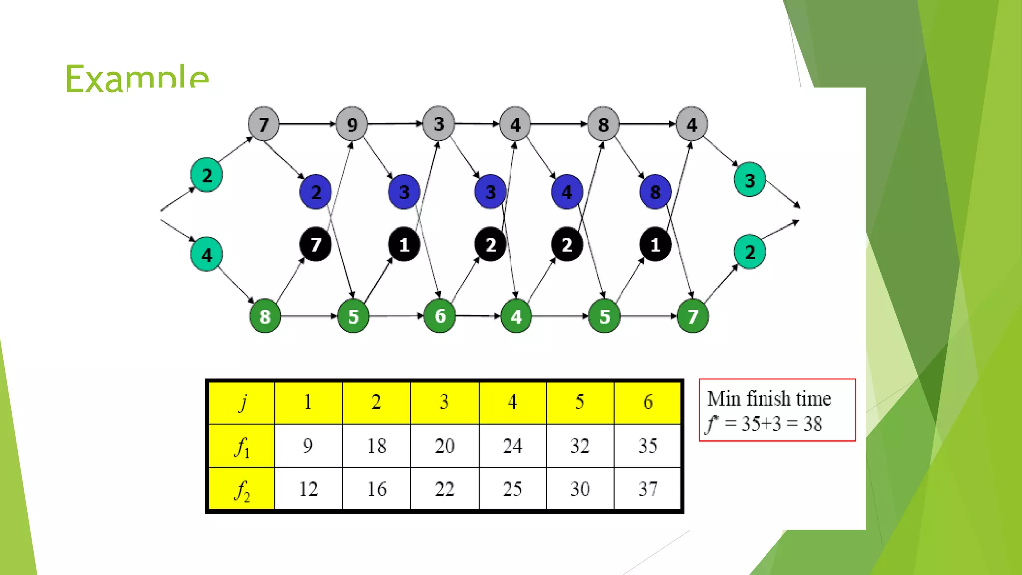
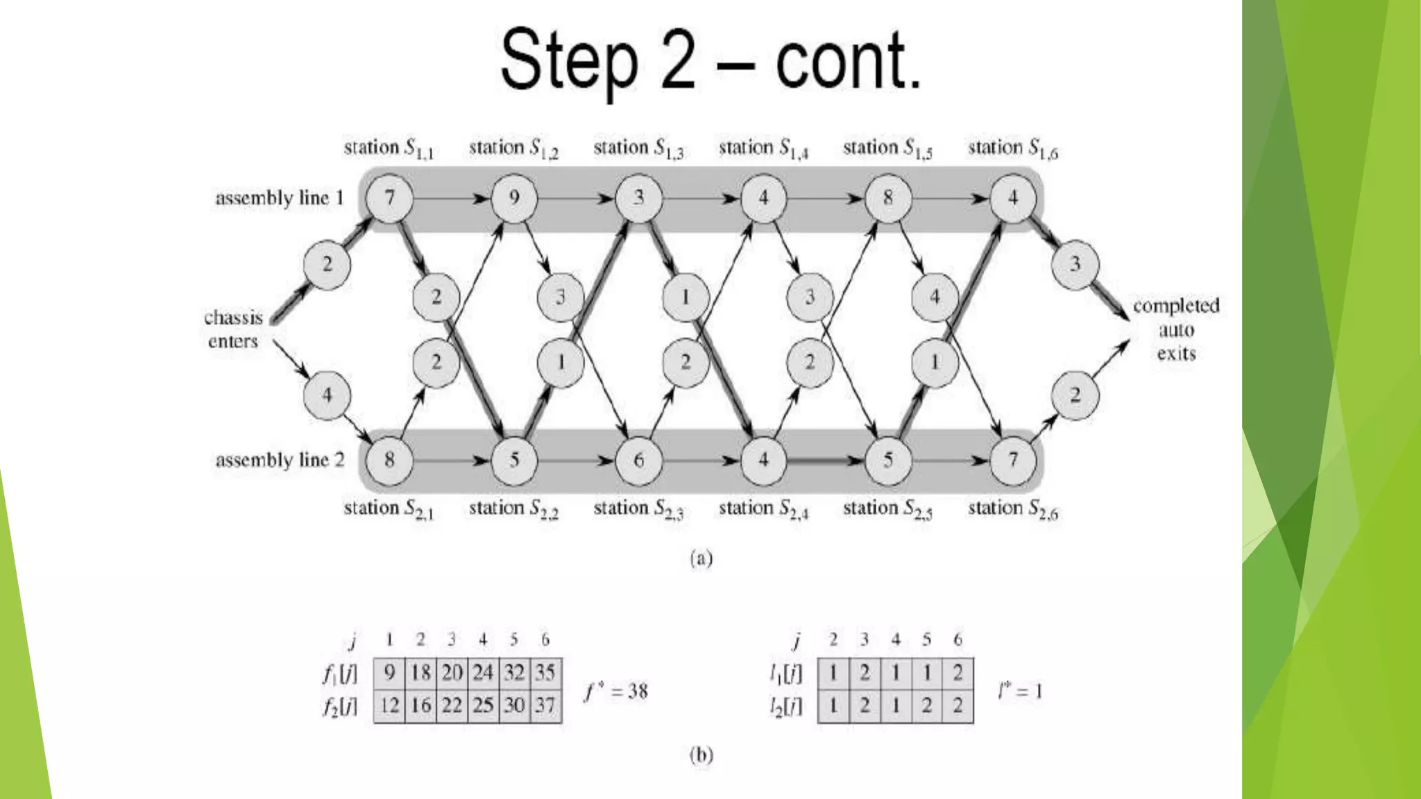
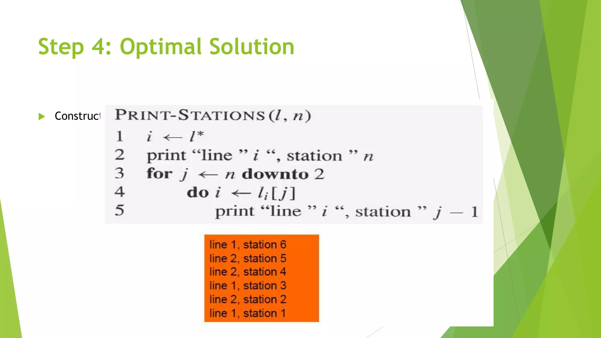
![Step 2: Recursive Solution
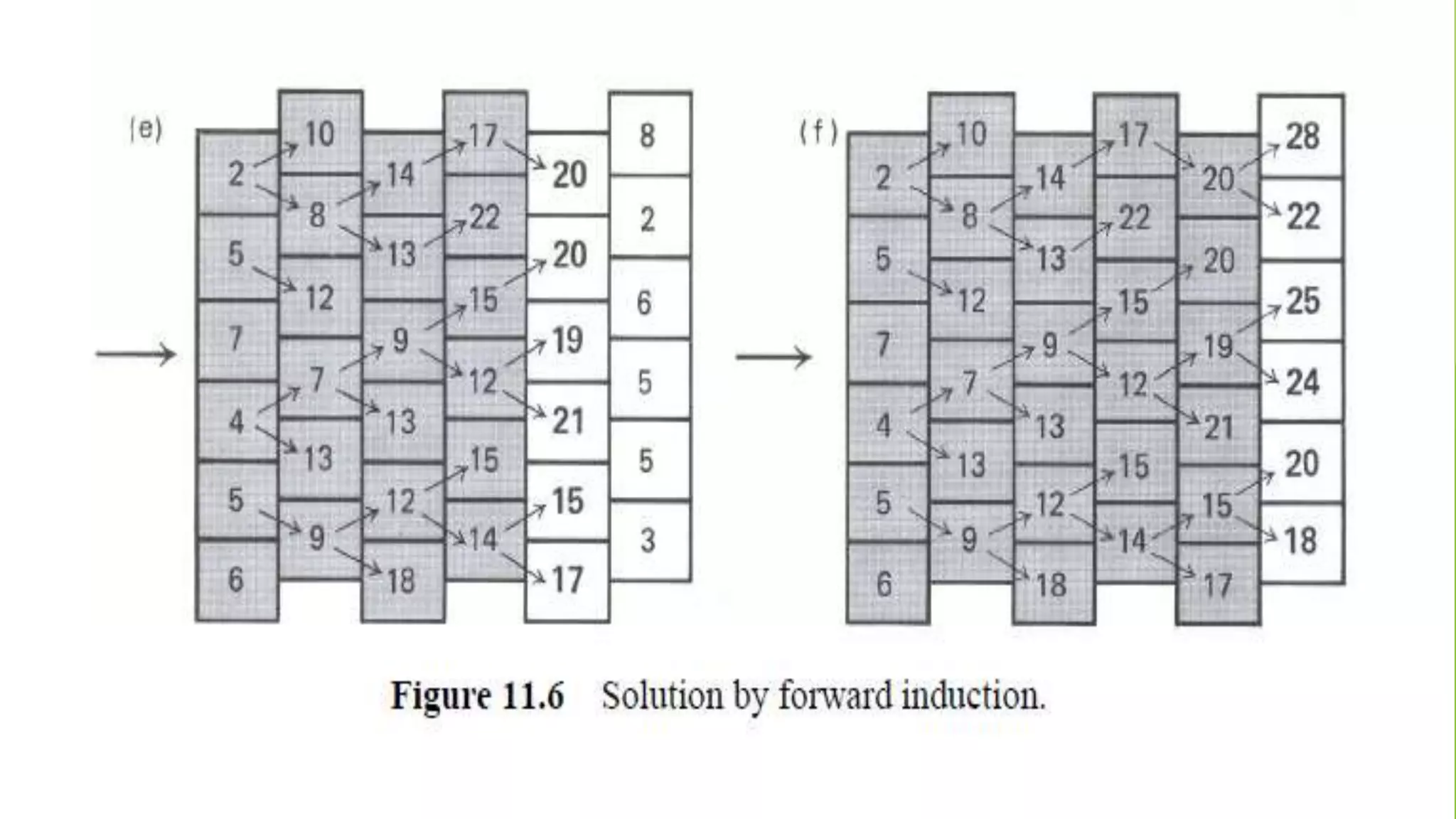
Using the values of l* and li[j] shown in Figure (b) in next slide, we would trace a
fastest way through the factory shown in part (a) as follows
The fastest total time comes from choosing stations
Line 1: 1, 3, & 6 Line 2: 2, 4, & 5](https://image.slidesharecdn.com/presentation1-150601195355-lva1-app6892/75/dynamic-programming-complete-by-Mumtaz-Ali-03154103173-70-2048.jpg)


![Pseudocode
1. int Chain( int i, int j )
2. {
3. int min = 10000, value, k;
4. if( i == j ){
5. return 0;
6. }
7. else{
8. for( k = i; k < j; k++ ){
9. value = (Chain(i, k) + Chain(k + 1, j) + (dimensions[i-1] *
dimensions[k] * dimensions[j]));
10. if( min > value ){
11. min = value;
12. mat[i][j] = k;
13. }
14. }
15. }
16. return min;](https://crownmelresort.com/image.slidesharecdn.com/presentation1-150601195355-lva1-app6892/75/dynamic-programming-complete-by-Mumtaz-Ali-03154103173-48-2048.jpg)
![1. int main(void)
2. {
3. int result, i;
4. printf("Enter number of matrices: ");
5. scanf("%d", &n);
6. printf("Enter dimensions : ");
7. for( i = 0; i <= n; i++ ){
8. scanf("%d", &dimensions[i]);
9. }
10. result = Chain(1, n);
11. printf("nTotal number of multiplications: %d andn", result);
12. printf("Multiplication order is: ");
13. PrintOrder( 1, n );
14. printf("n");
15. }](https://crownmelresort.com/image.slidesharecdn.com/presentation1-150601195355-lva1-app6892/75/dynamic-programming-complete-by-Mumtaz-Ali-03154103173-49-2048.jpg)


![Step 2: Recursive Solution
Define the value of an optimal solution recursively in terms of the
optimal solution to sub-problems
Sub-problem here
finding the fastest way through station j on both lines (i=1,2)
Let fi [j] be the fastest possible time to go from starting point through Si,j
The fastest time to go all the way through the factory: f*
x1 and x2 are the exit times from lines 1 and 2, respectively](https://crownmelresort.com/image.slidesharecdn.com/presentation1-150601195355-lva1-app6892/75/dynamic-programming-complete-by-Mumtaz-Ali-03154103173-65-2048.jpg)


![Step 2: Recursive Solution
To help us keep track of how to construct an optimal solution, let us define
li[j ]: line # whose station j-1 is used in a fastest way through Si,j (i = 1, 2, and j =
2, 3,..., n)
we avoid defining li[1] because no station precedes station 1 on either lines.
We also define
l*: the line whose station n is used in a fastest way through the entire factory](https://crownmelresort.com/image.slidesharecdn.com/presentation1-150601195355-lva1-app6892/75/dynamic-programming-complete-by-Mumtaz-Ali-03154103173-69-2048.jpg)
![Step 2: Recursive Solution
Using the values of l* and li[j] shown in Figure (b) in next slide, we would trace a
fastest way through the factory shown in part (a) as follows
The fastest total time comes from choosing stations
Line 1: 1, 3, & 6 Line 2: 2, 4, & 5](https://crownmelresort.com/image.slidesharecdn.com/presentation1-150601195355-lva1-app6892/75/dynamic-programming-complete-by-Mumtaz-Ali-03154103173-70-2048.jpg)


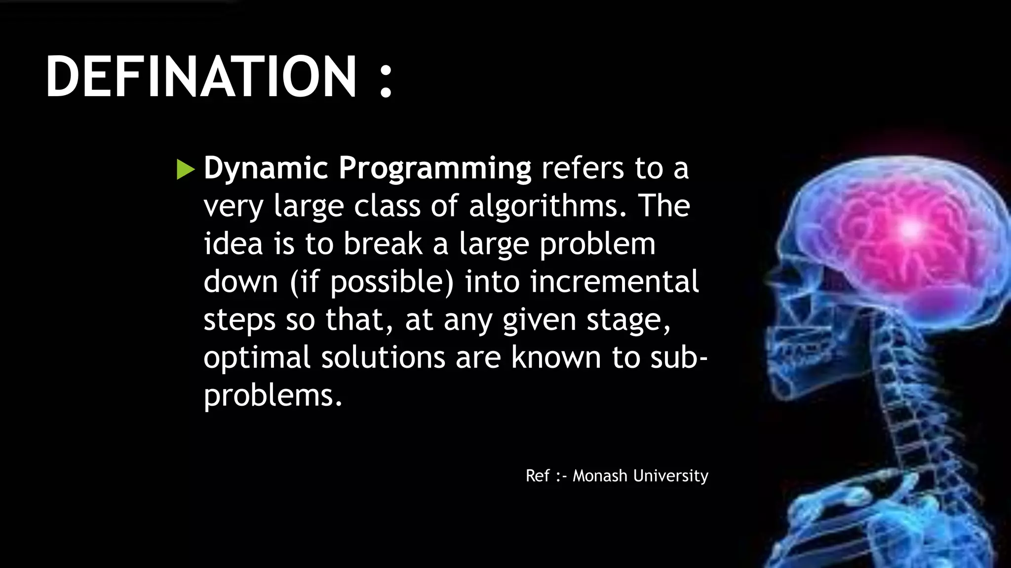
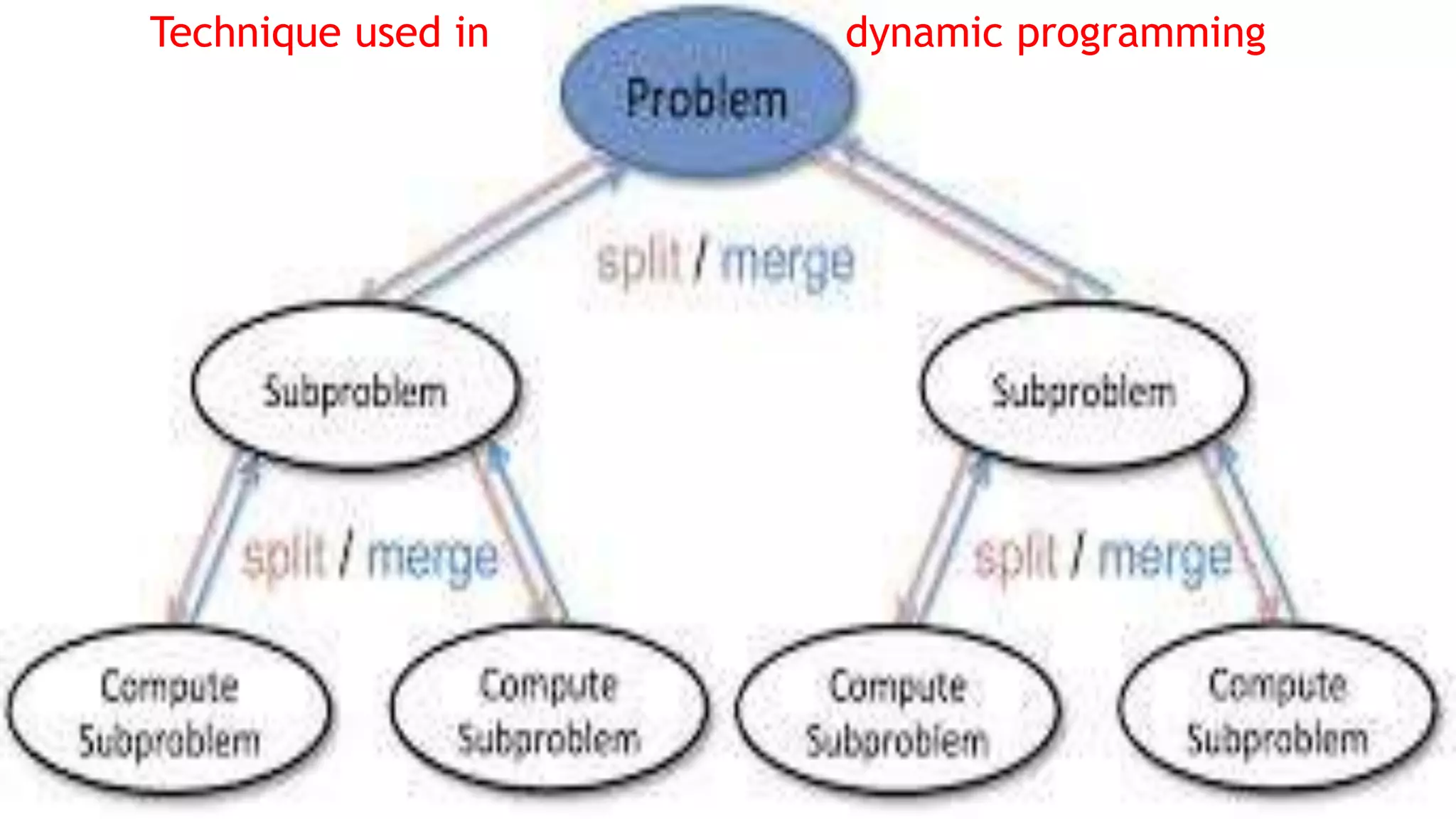
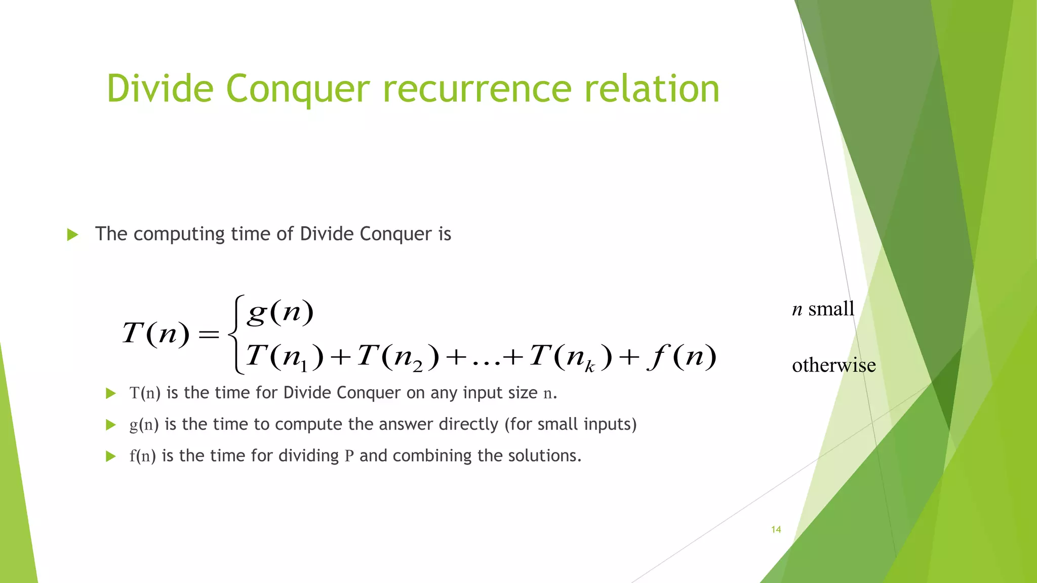
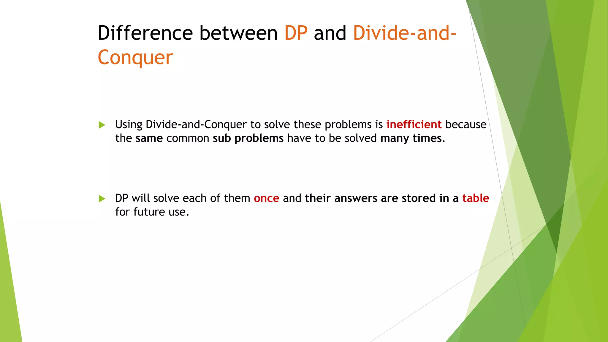
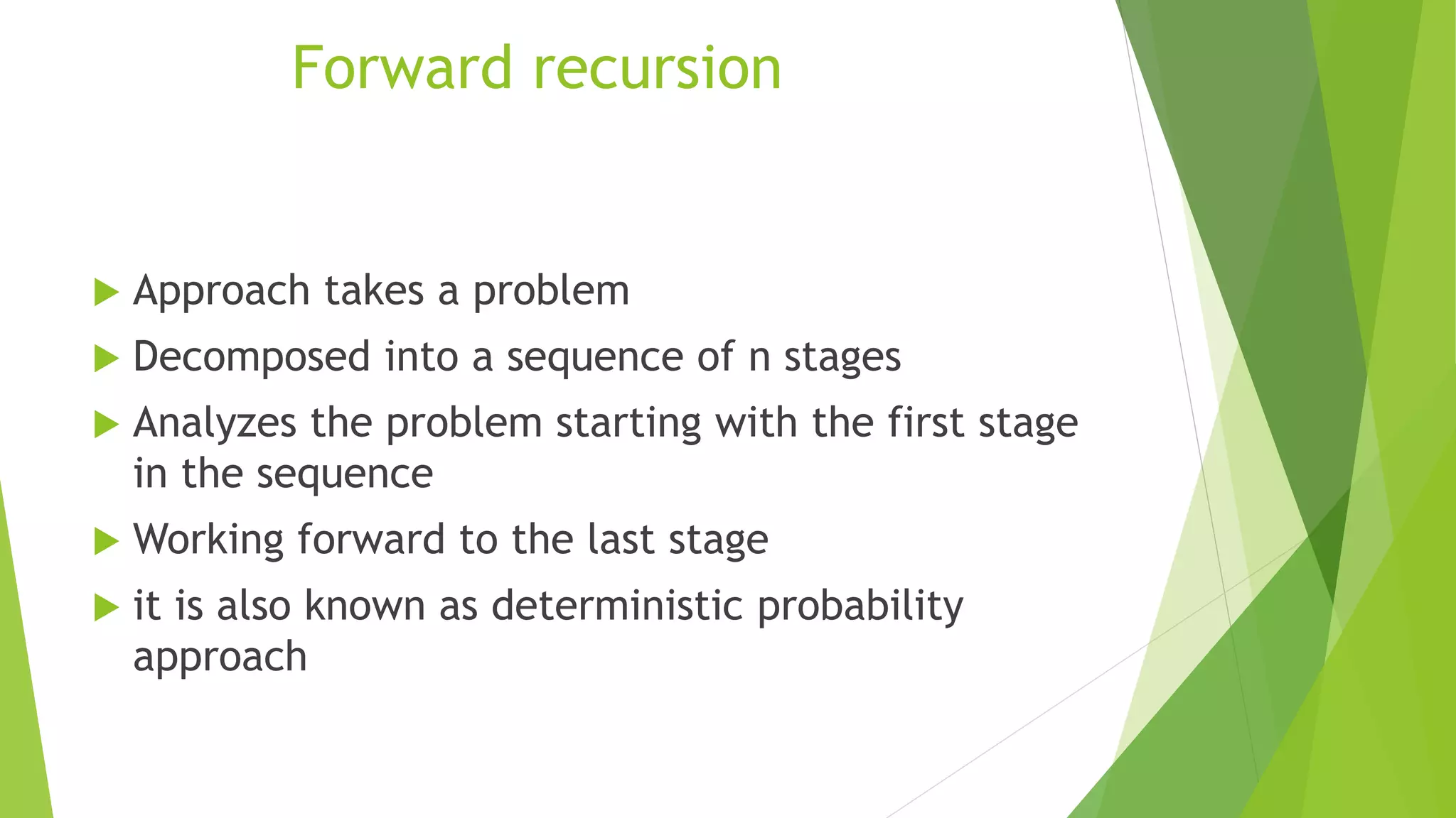
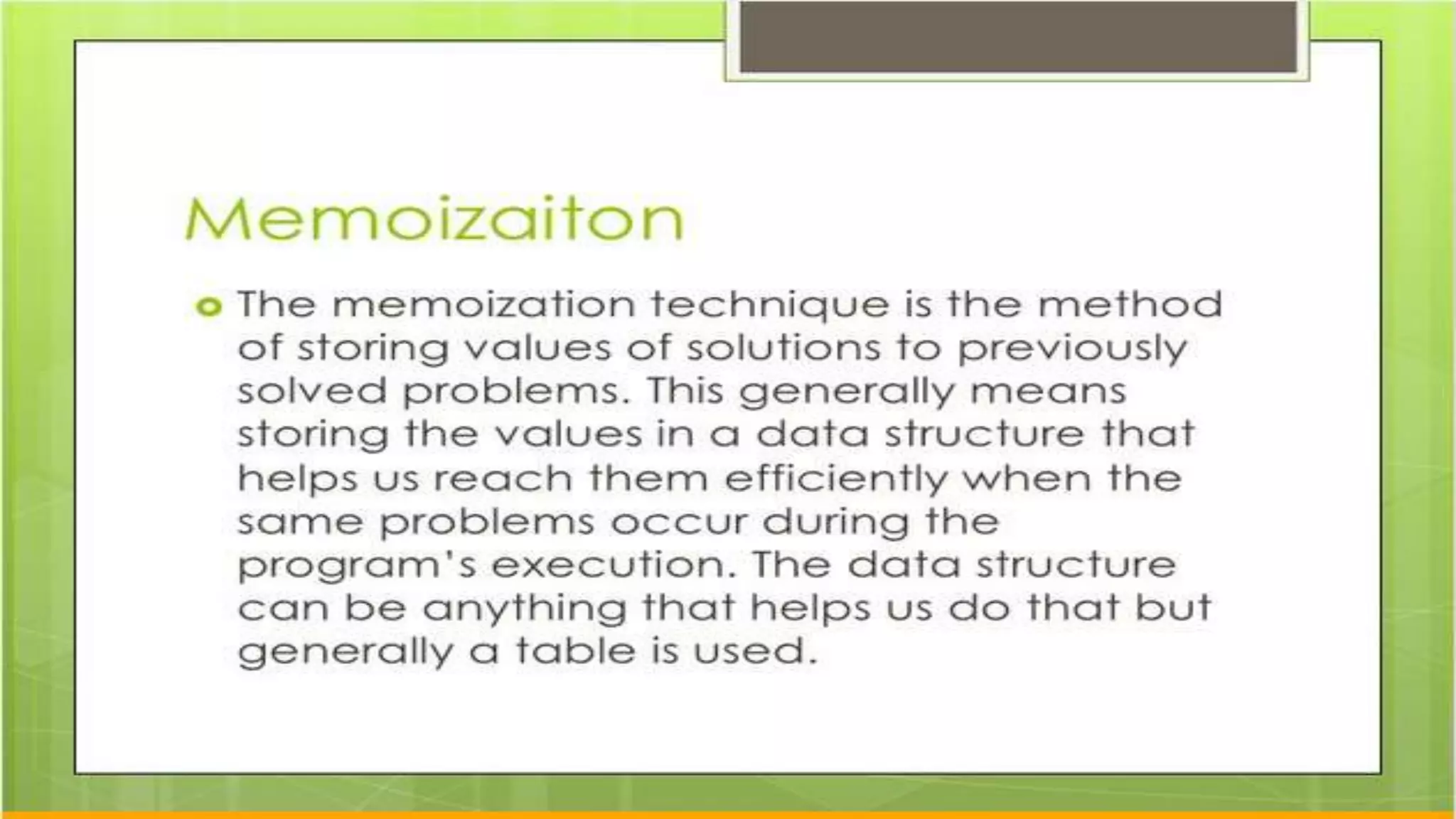
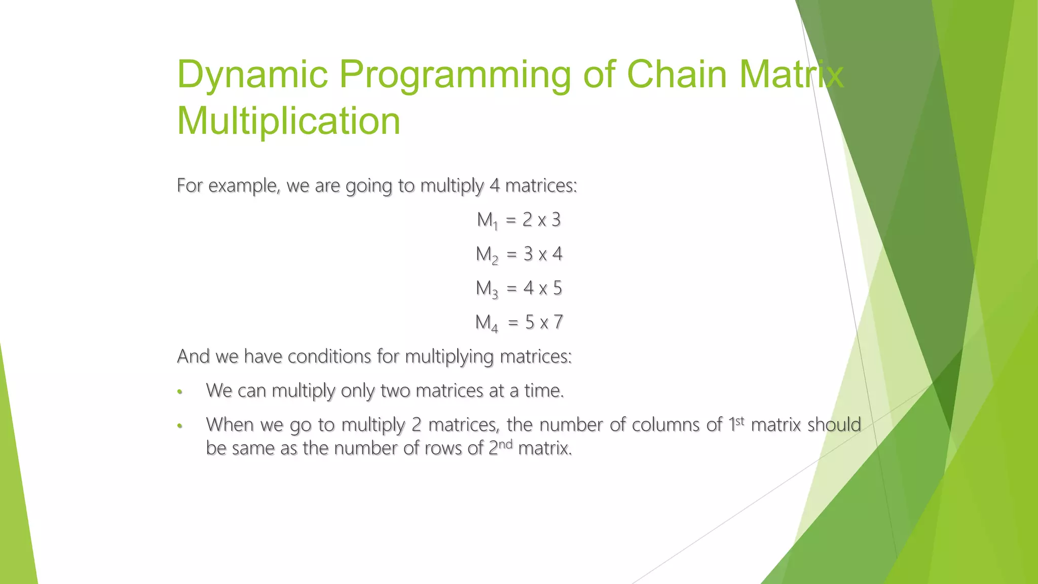
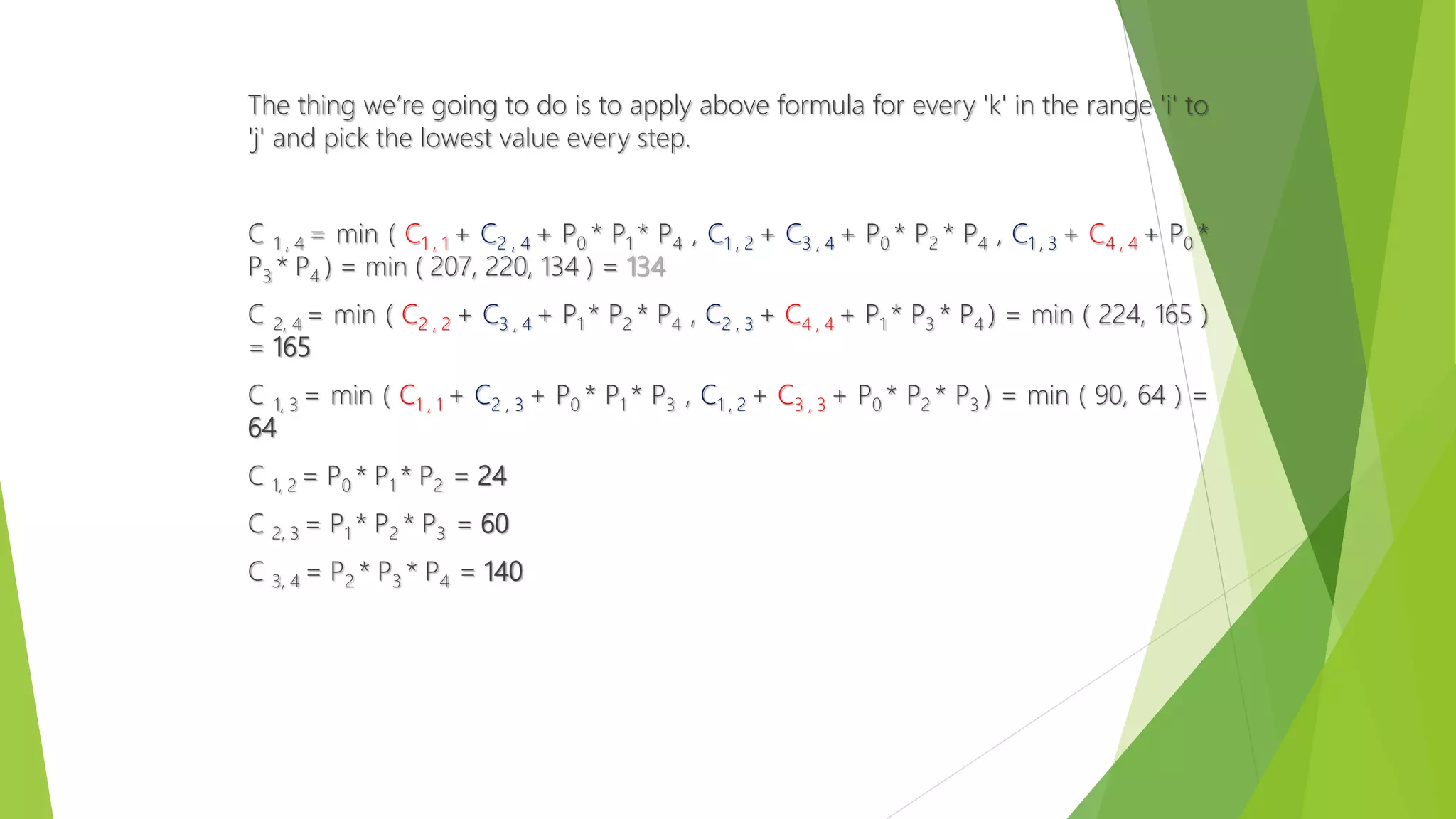
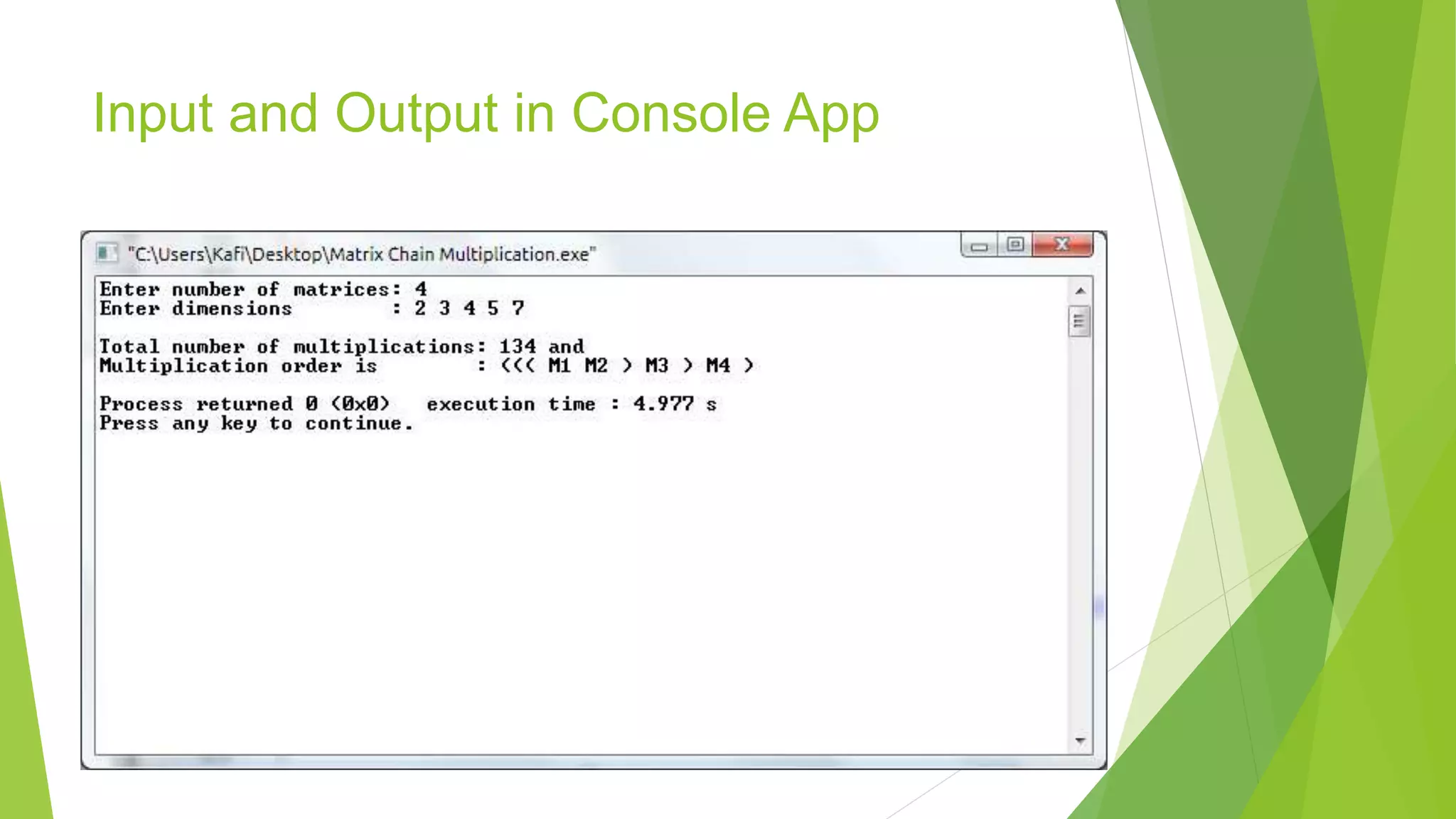
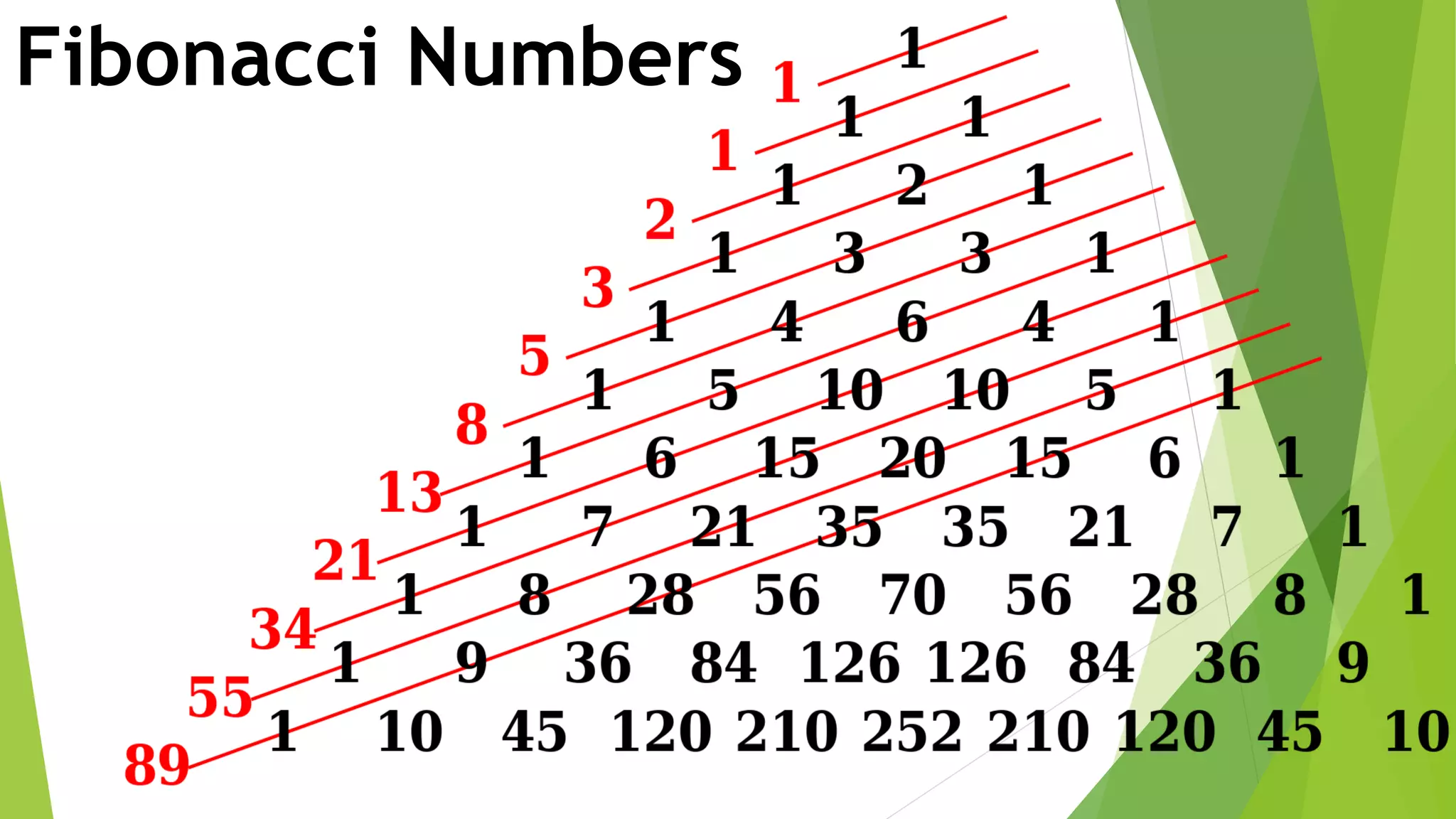
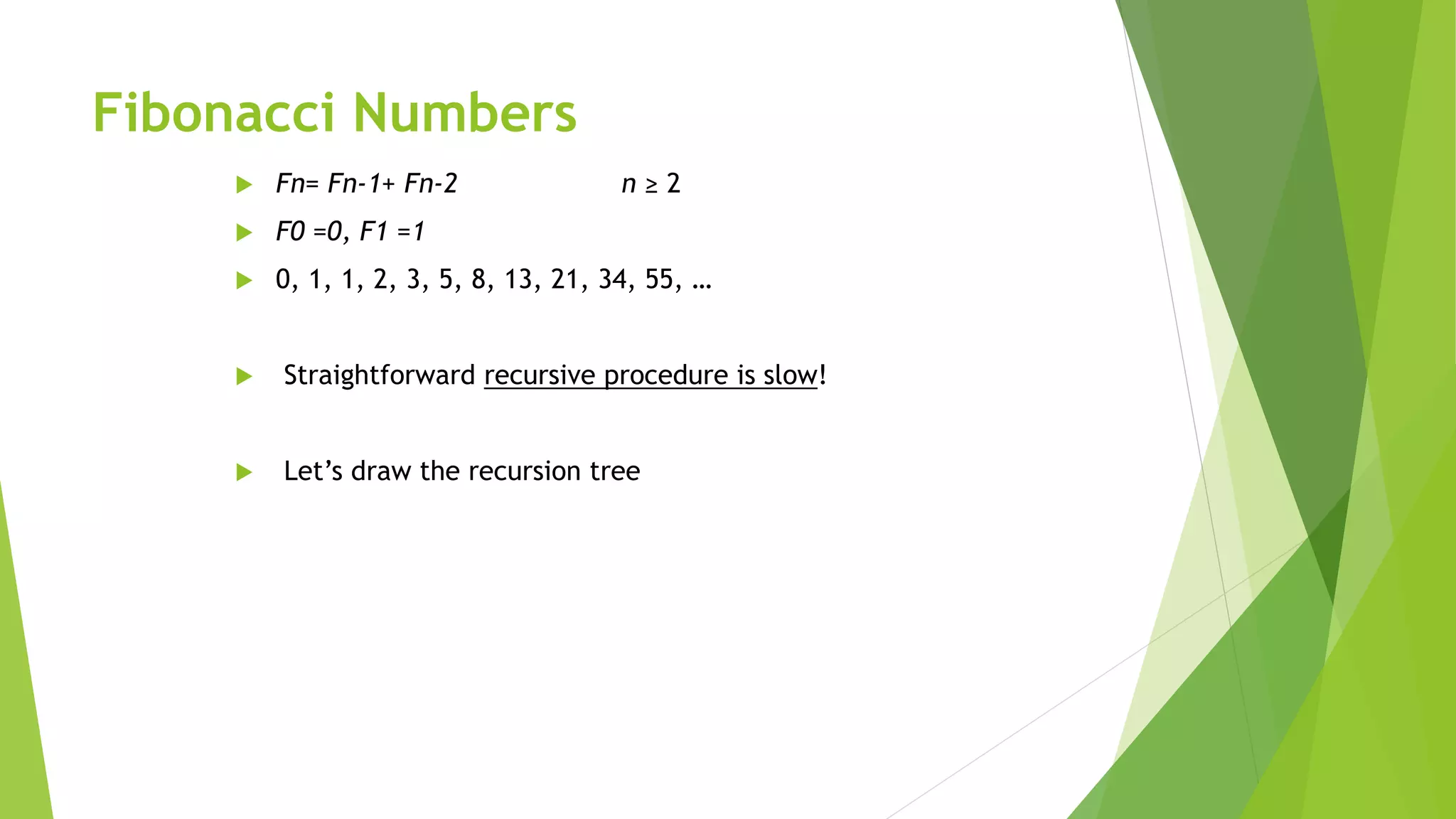
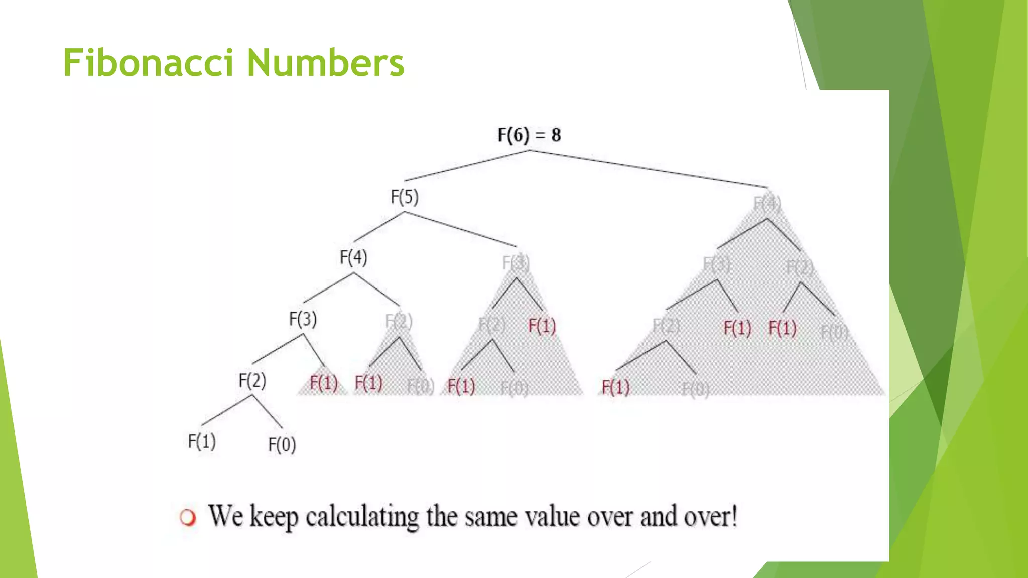
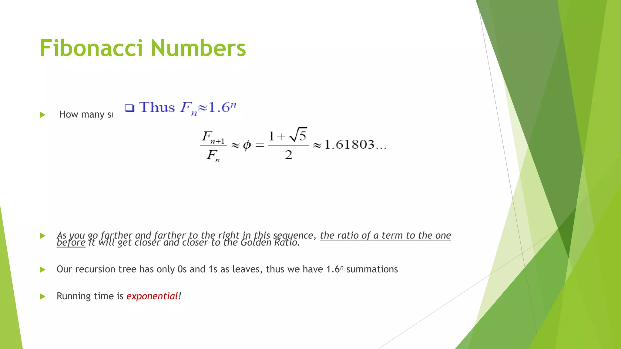
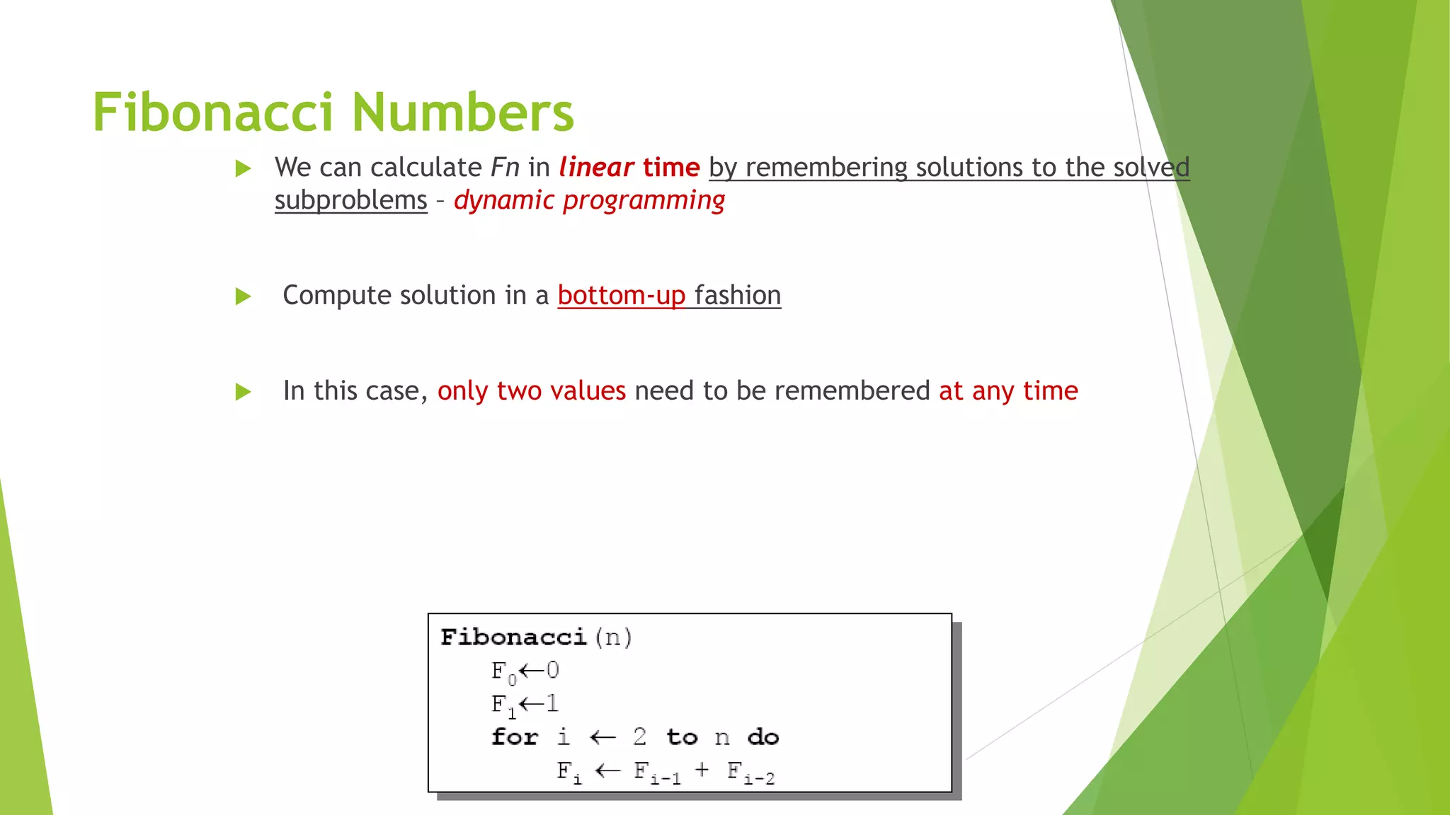
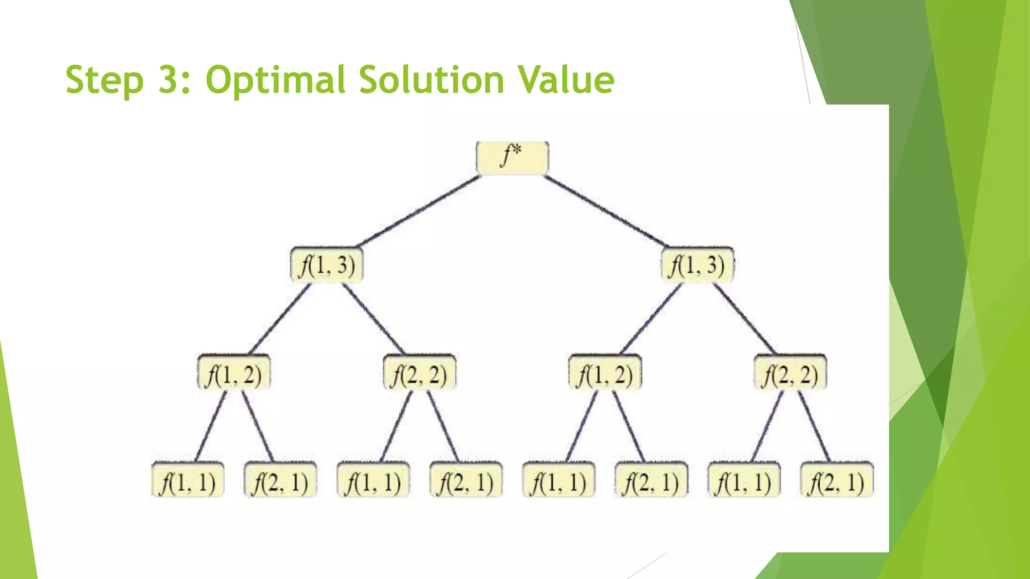
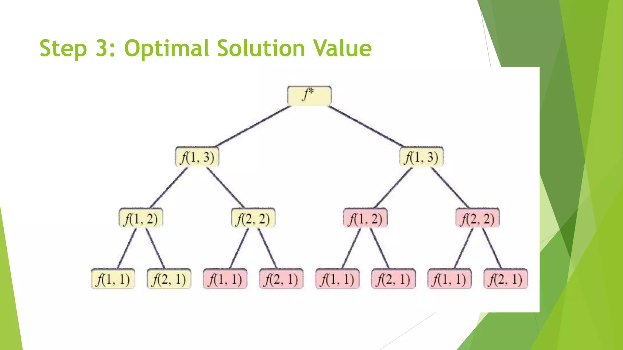
The document discusses dynamic programming, including its meaning, definition, uses, techniques, and examples. Dynamic programming refers to breaking large problems down into smaller subproblems, solving each subproblem only once, and storing the results for future use. This avoids recomputing the same subproblems repeatedly. Examples covered include matrix chain multiplication, the Fibonacci sequence, and optimal substructure. The document provides details on formulating and solving dynamic programming problems through recursive definitions and storing results in tables.


![ANPARA THERMAL POWER STATION[1] sangam.pdf](https://cdn.slidesharecdn.com/ss_thumbnails/anparathermalpowerstation1sangam-251121115219-9261cde4-thumbnail.jpg?width=640&height=640&fit=bounds)


