Downloaded 606 times
![Finding Minimum or Maximum Alg.: MINIMUM (A, n) min ← A[1] for i ← 2 to n do if min > A[i] then min ← A[i] return min How many comparisons are needed? n – 1 : each element, except the minimum, must be compared to a smaller element at least once The same number of comparisons are needed to find the maximum The algorithm is optimal with respect to the number of comparisons performed](https://image.slidesharecdn.com/lecture8dynamicprogramming-101206135908-phpapp02/75/Lecture-8-dynamic-programming-3-2048.jpg)
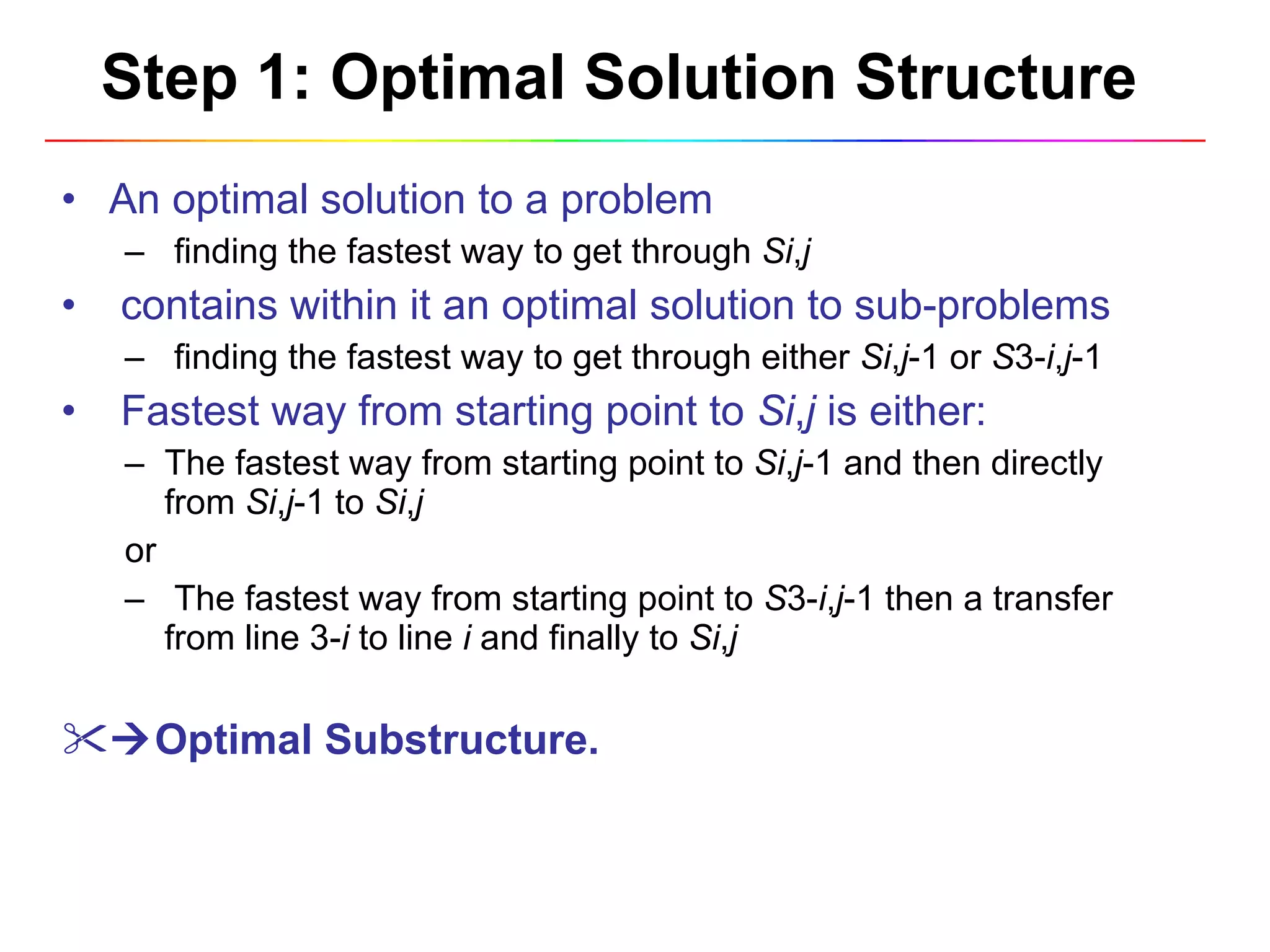
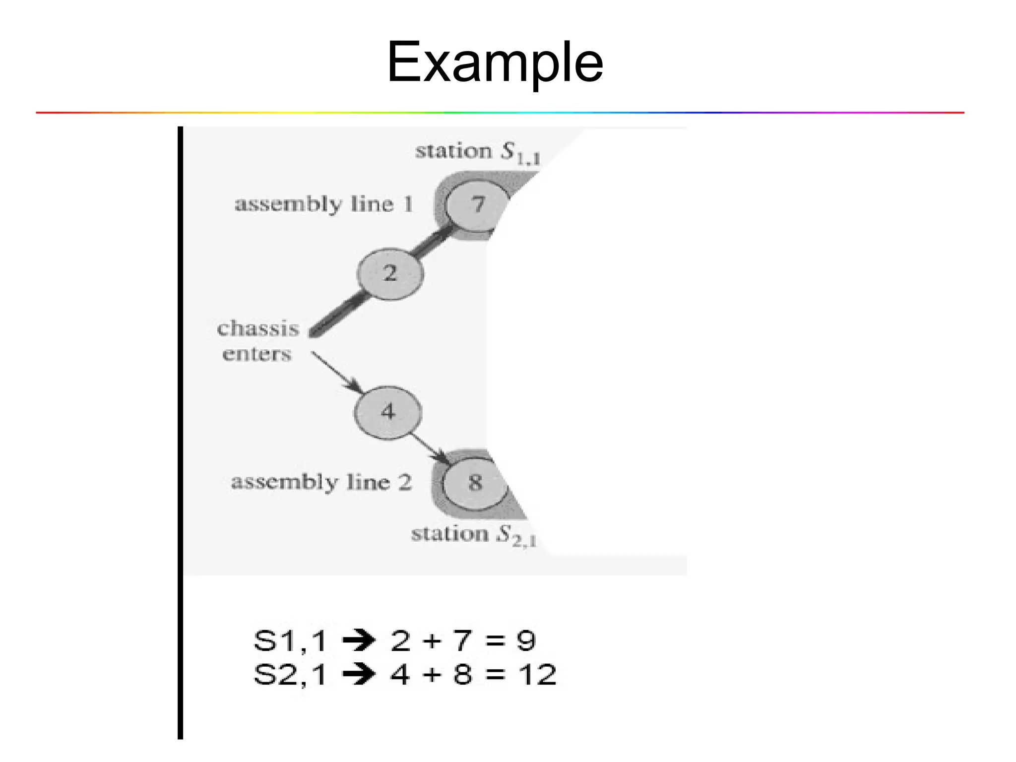
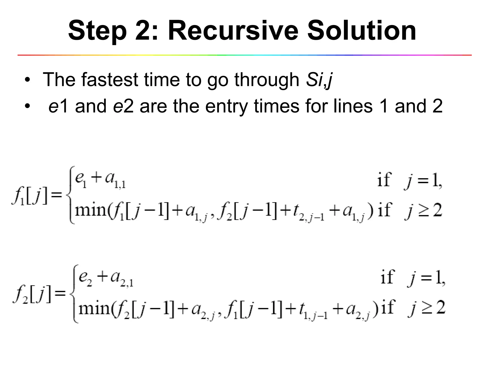
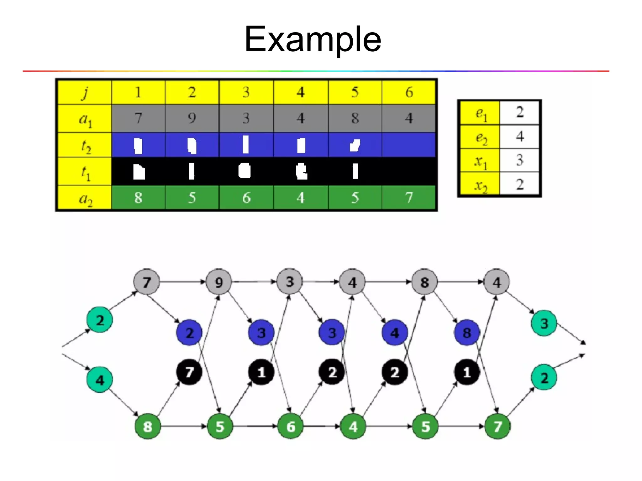
![Step 2: Recursive Solution Define the value of an optimal solution recursively in terms of the optimal solution to sub-problems Sub-problem here finding the fastest way through station j on both lines (i=1,2) Let fi [ j ] be the fastest possible time to go from starting point through Si , j The fastest time to go all the way through the factory : f * x 1 and x 2 are the exit times from lines 1 and 2, respectively](https://image.slidesharecdn.com/lecture8dynamicprogramming-101206135908-phpapp02/75/Lecture-8-dynamic-programming-29-2048.jpg)
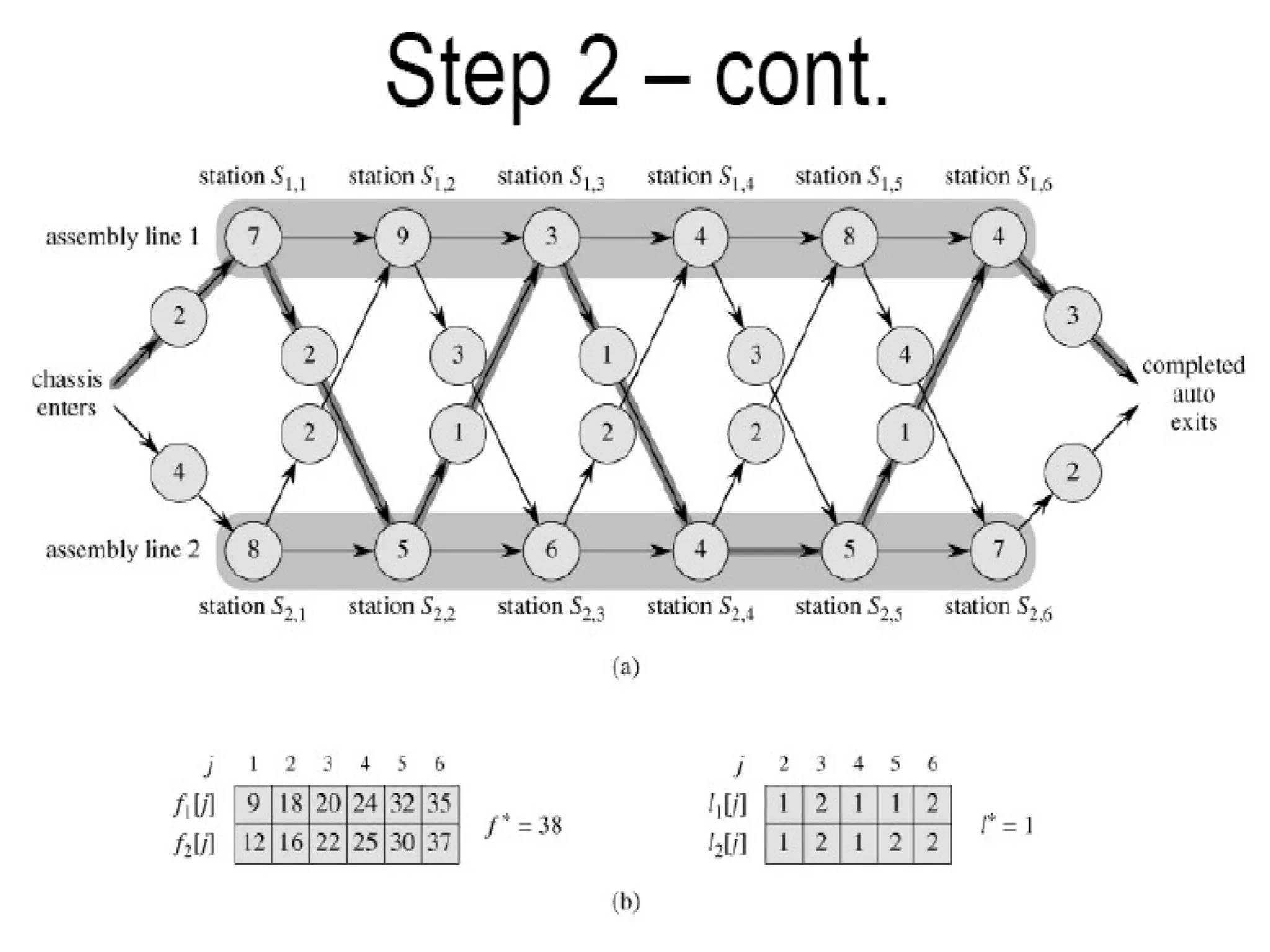
![Step 2: Recursive Solution To help us keep track of how to construct an optimal solution, let us define li [ j ]: line # whose station j -1 is used in a fastest way through Si , j ( i = 1, 2, and j = 2, 3,..., n ) we avoid defining li [1] because no station precedes station 1 on either lines. We also define l *: the line whose station n is used in a fastest way through the entire factory](https://image.slidesharecdn.com/lecture8dynamicprogramming-101206135908-phpapp02/75/Lecture-8-dynamic-programming-33-2048.jpg)
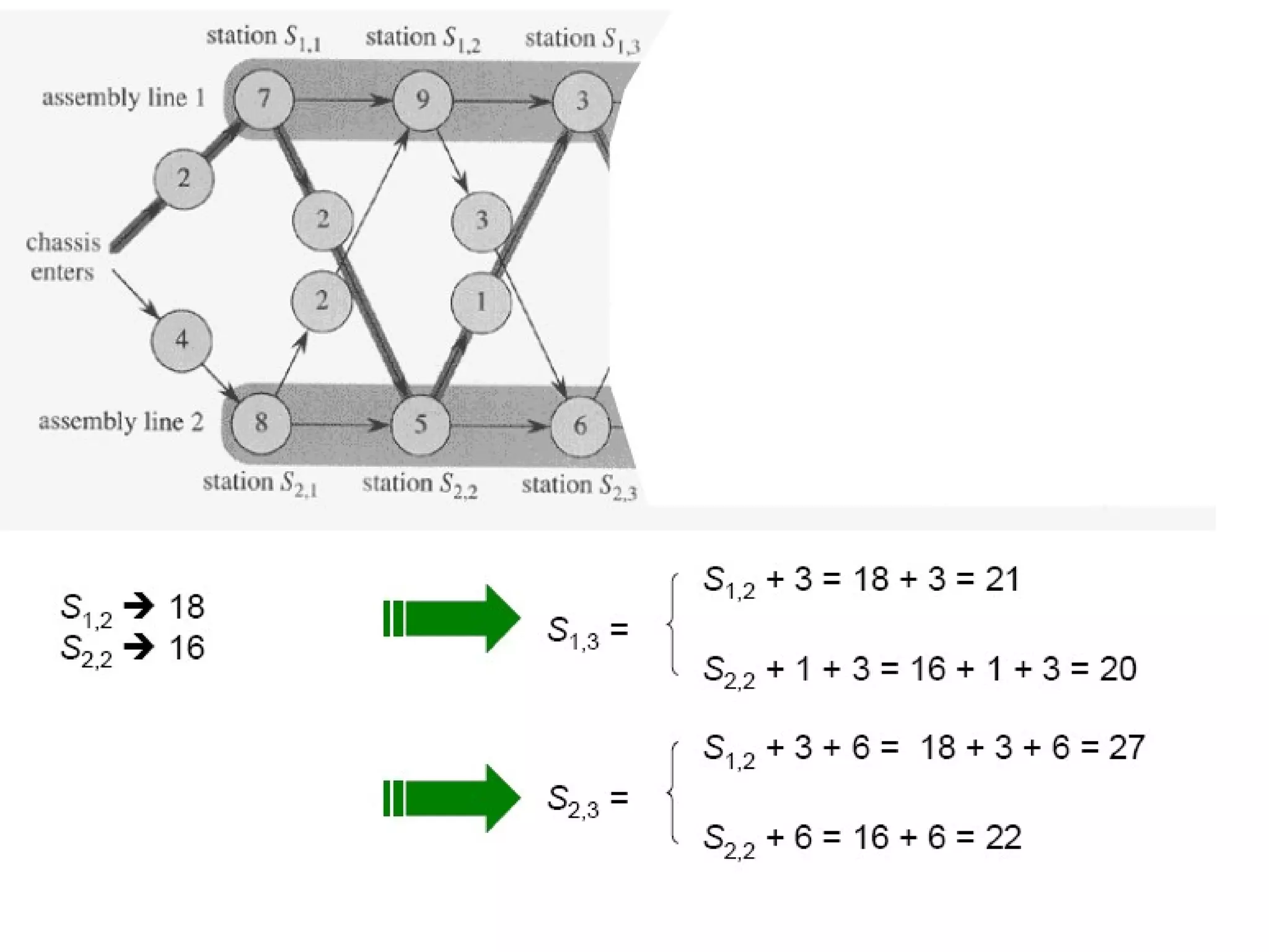
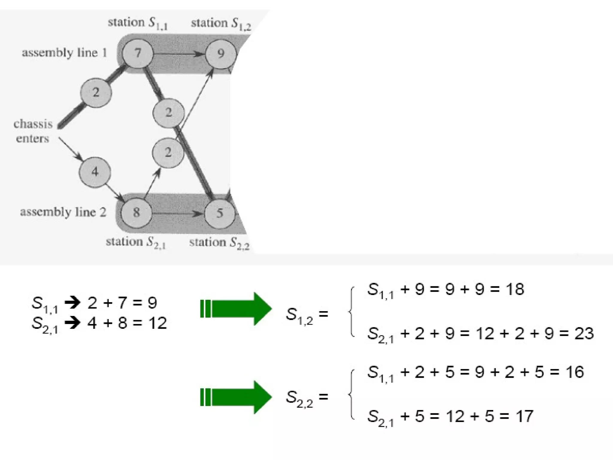
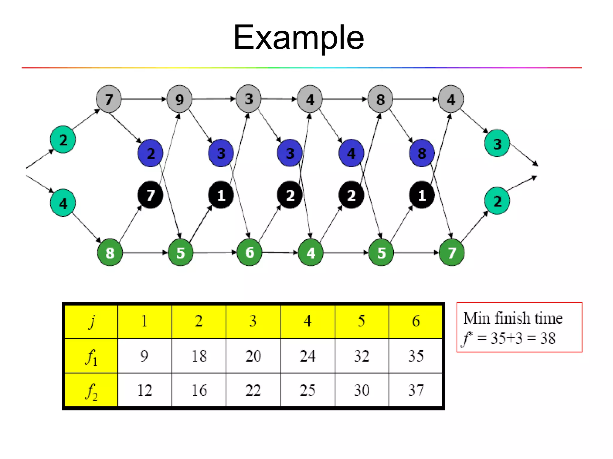
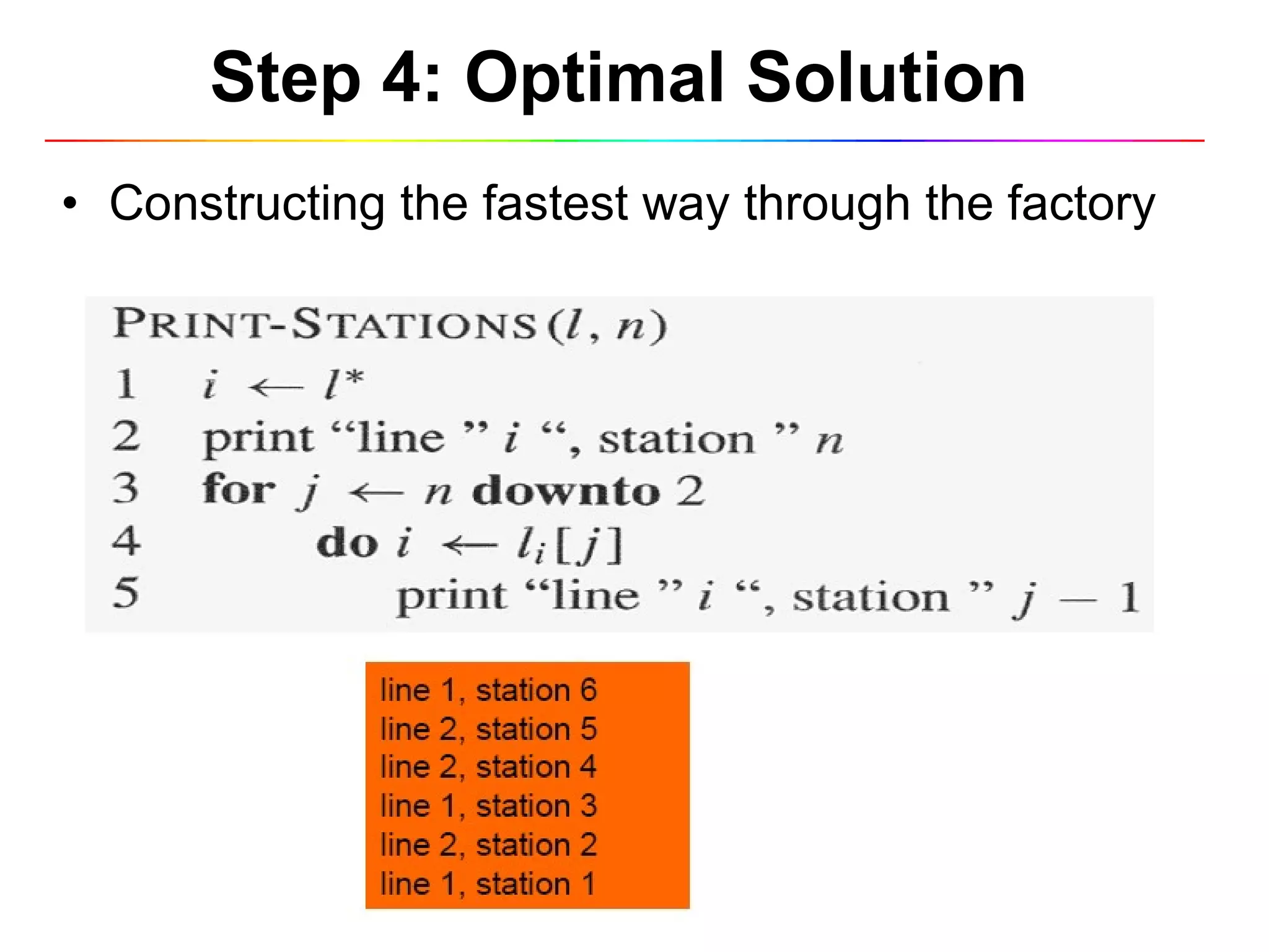
![Step 2: Recursive Solution Using the values of l * and li [ j ] shown in Figure (b) in next slide, we would trace a fastest way through the factory shown in part (a) as follows The fastest total time comes from choosing stations Line 1: 1, 3, & 6 Line 2: 2, 4, & 5](https://image.slidesharecdn.com/lecture8dynamicprogramming-101206135908-phpapp02/75/Lecture-8-dynamic-programming-34-2048.jpg)


![Finding Minimum or Maximum Alg.: MINIMUM (A, n) min ← A[1] for i ← 2 to n do if min > A[i] then min ← A[i] return min How many comparisons are needed? n – 1 : each element, except the minimum, must be compared to a smaller element at least once The same number of comparisons are needed to find the maximum The algorithm is optimal with respect to the number of comparisons performed](https://crownmelresort.com/image.slidesharecdn.com/lecture8dynamicprogramming-101206135908-phpapp02/75/Lecture-8-dynamic-programming-3-2048.jpg)


![Step 2: Recursive Solution Define the value of an optimal solution recursively in terms of the optimal solution to sub-problems Sub-problem here finding the fastest way through station j on both lines (i=1,2) Let fi [ j ] be the fastest possible time to go from starting point through Si , j The fastest time to go all the way through the factory : f * x 1 and x 2 are the exit times from lines 1 and 2, respectively](https://crownmelresort.com/image.slidesharecdn.com/lecture8dynamicprogramming-101206135908-phpapp02/75/Lecture-8-dynamic-programming-29-2048.jpg)


![Step 2: Recursive Solution To help us keep track of how to construct an optimal solution, let us define li [ j ]: line # whose station j -1 is used in a fastest way through Si , j ( i = 1, 2, and j = 2, 3,..., n ) we avoid defining li [1] because no station precedes station 1 on either lines. We also define l *: the line whose station n is used in a fastest way through the entire factory](https://crownmelresort.com/image.slidesharecdn.com/lecture8dynamicprogramming-101206135908-phpapp02/75/Lecture-8-dynamic-programming-33-2048.jpg)
![Step 2: Recursive Solution Using the values of l * and li [ j ] shown in Figure (b) in next slide, we would trace a fastest way through the factory shown in part (a) as follows The fastest total time comes from choosing stations Line 1: 1, 3, & 6 Line 2: 2, 4, & 5](https://crownmelresort.com/image.slidesharecdn.com/lecture8dynamicprogramming-101206135908-phpapp02/75/Lecture-8-dynamic-programming-34-2048.jpg)


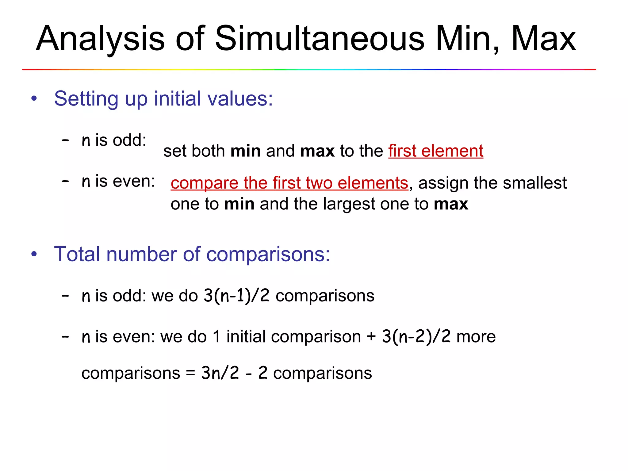
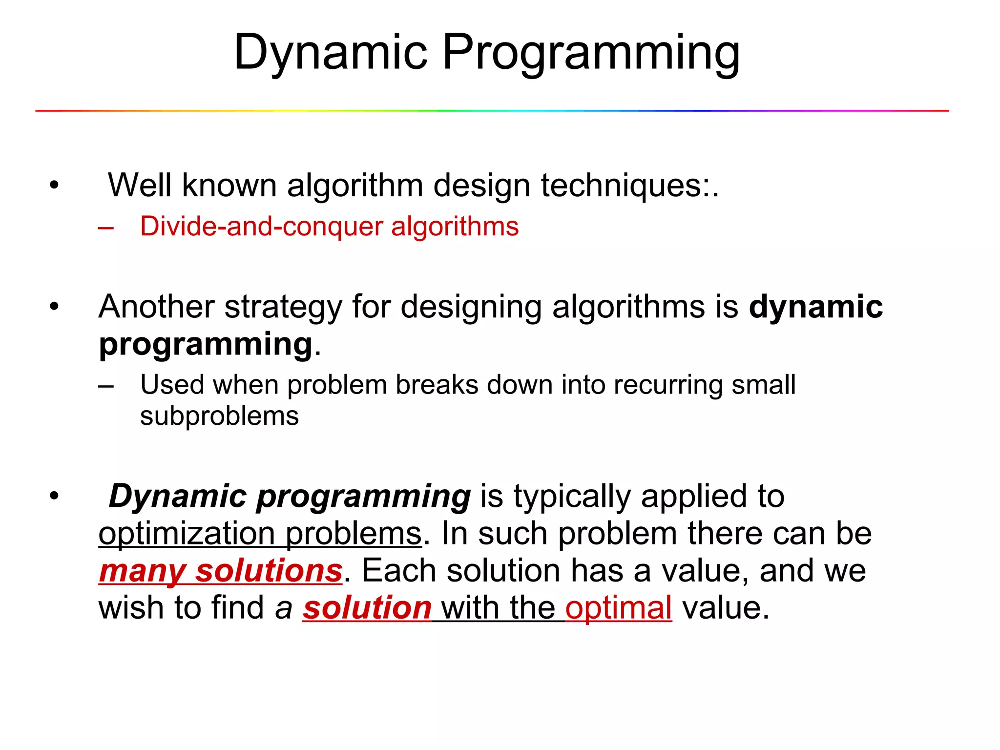
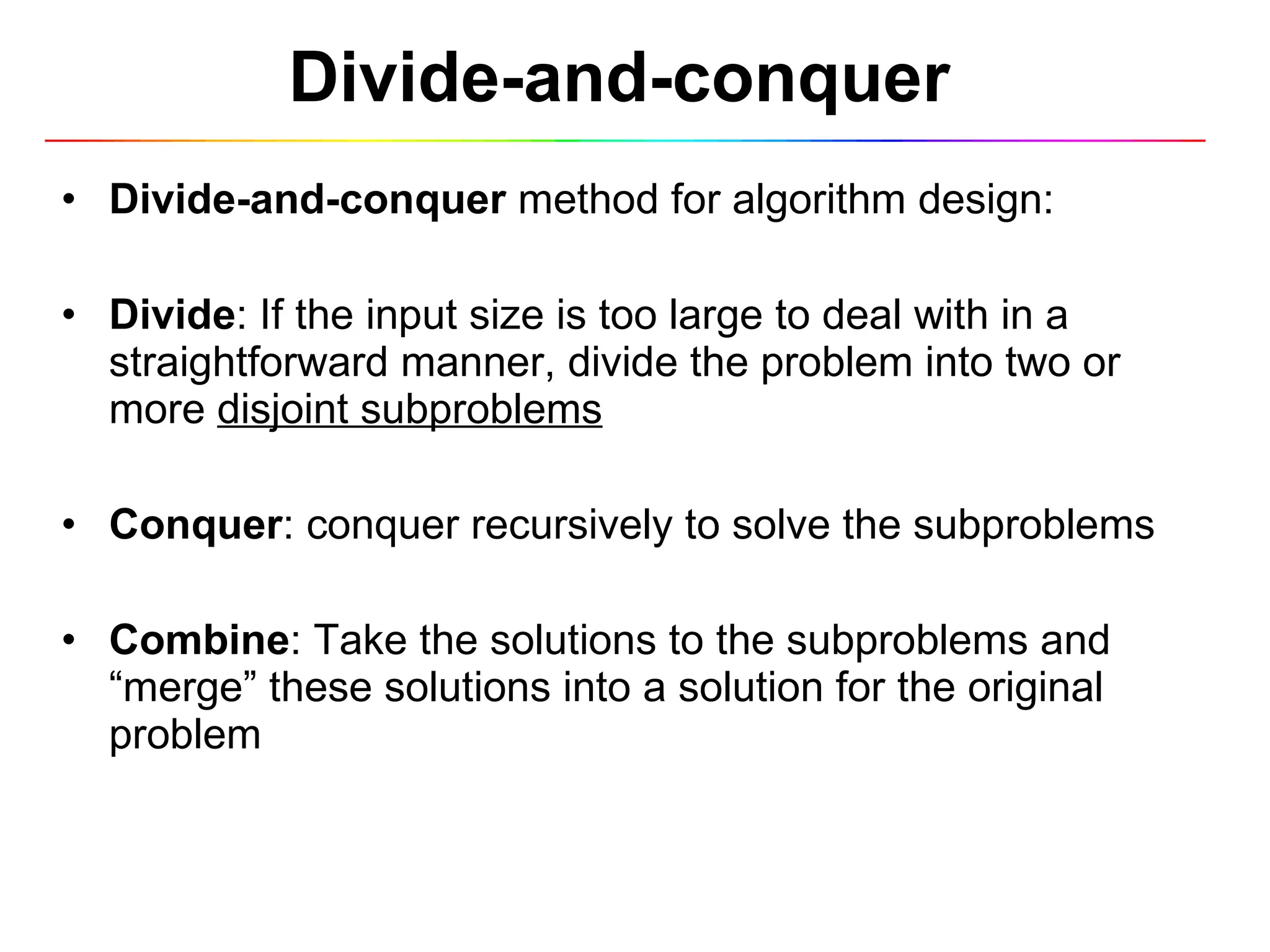
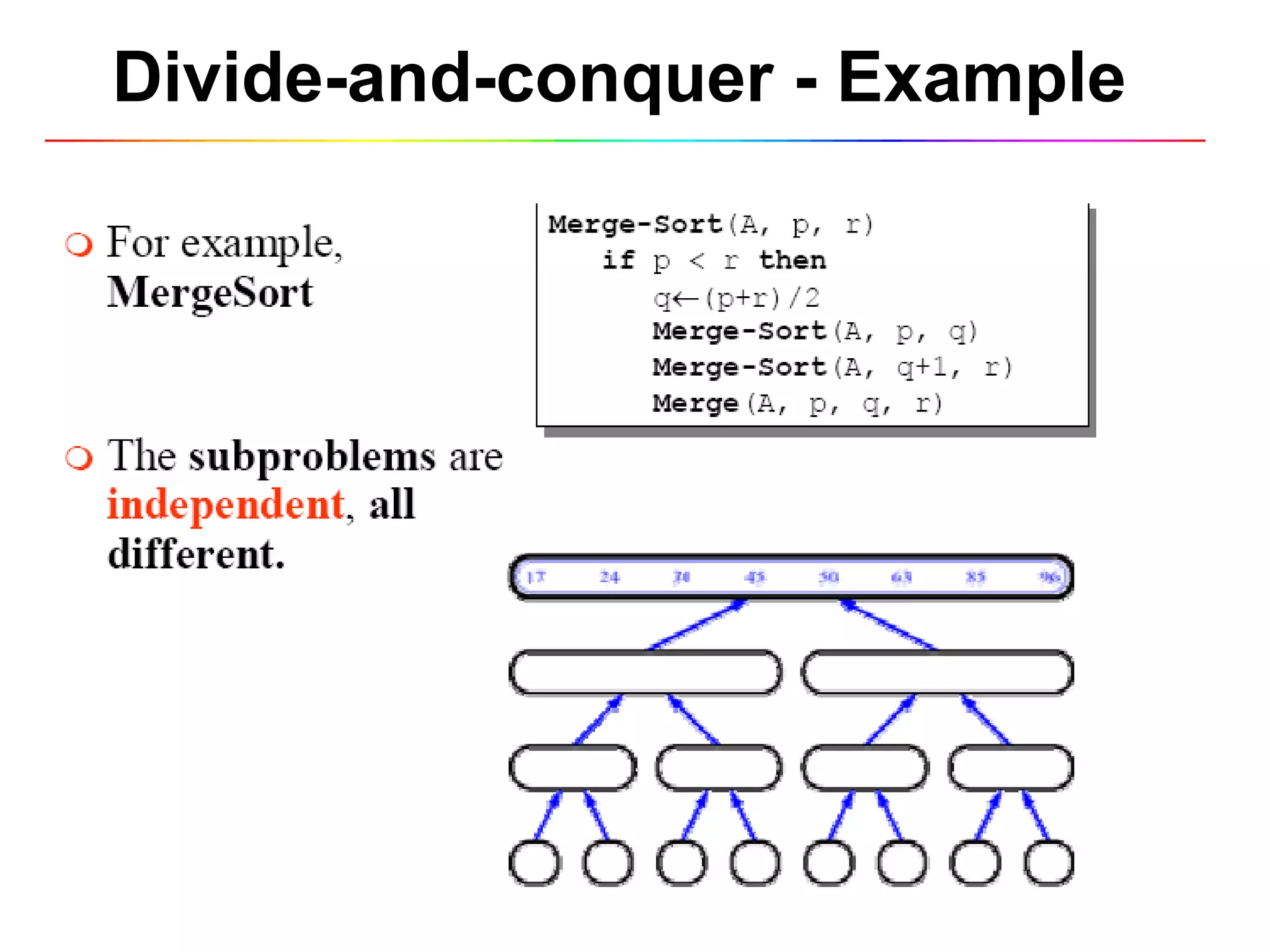
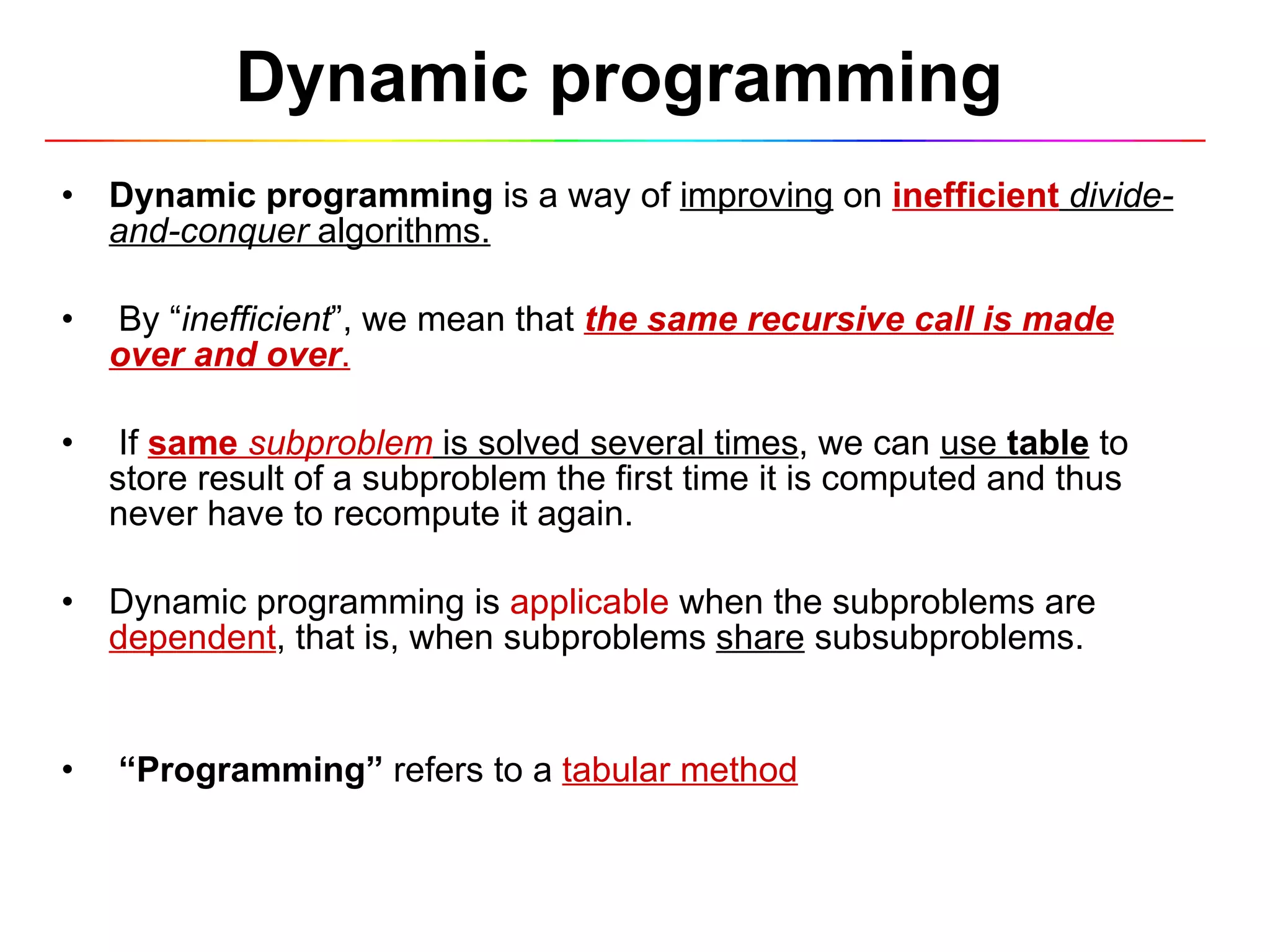
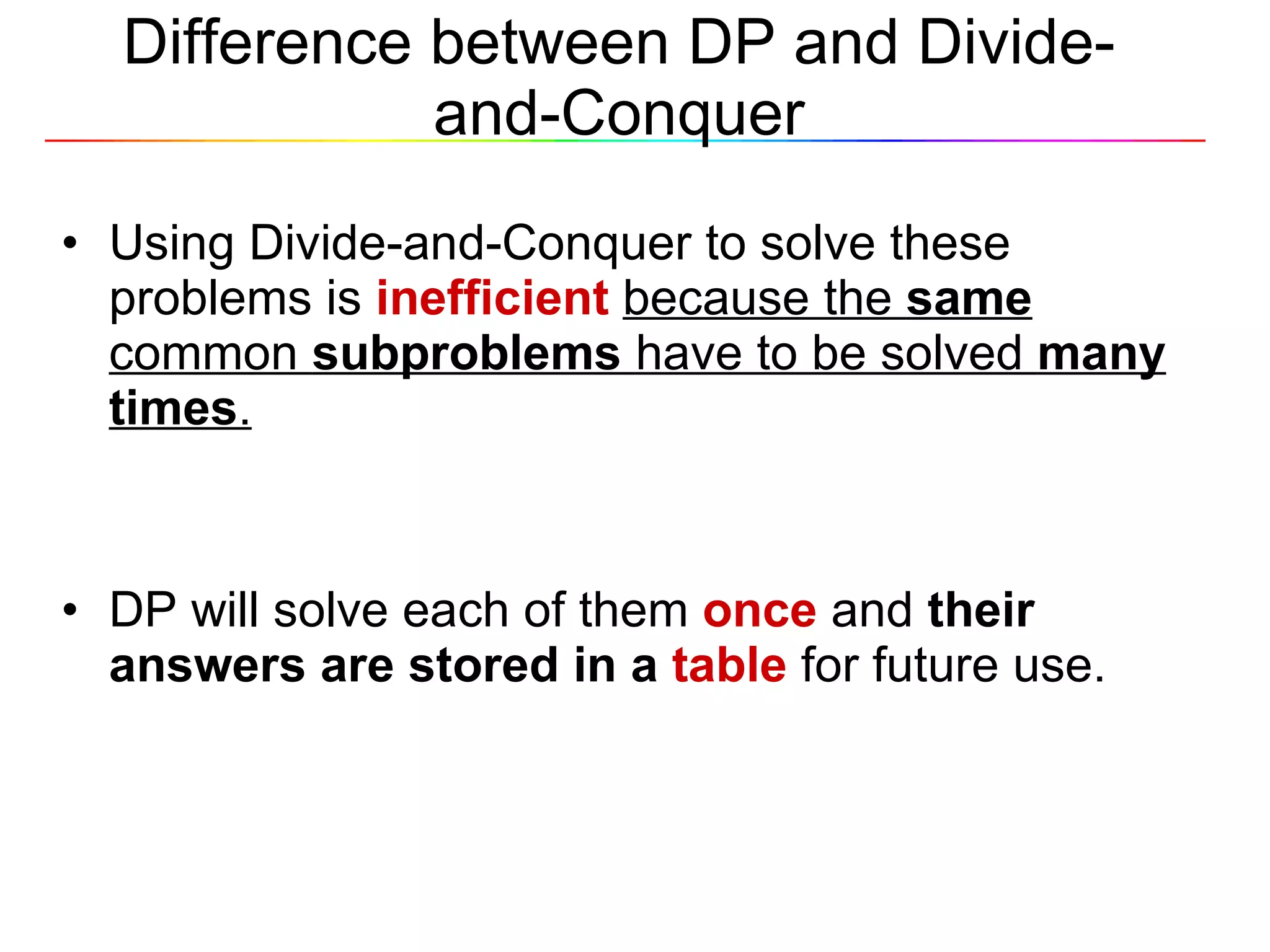
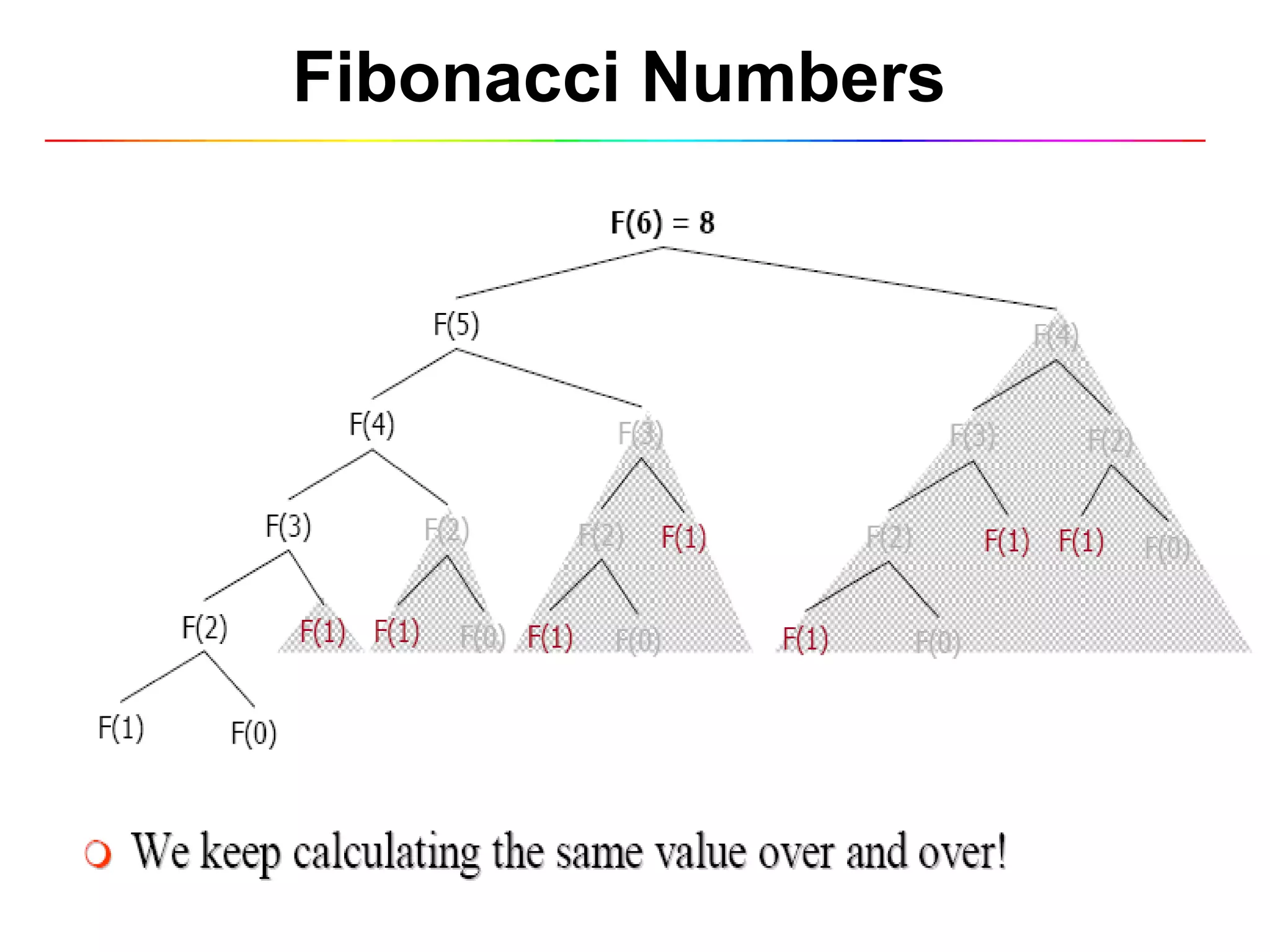
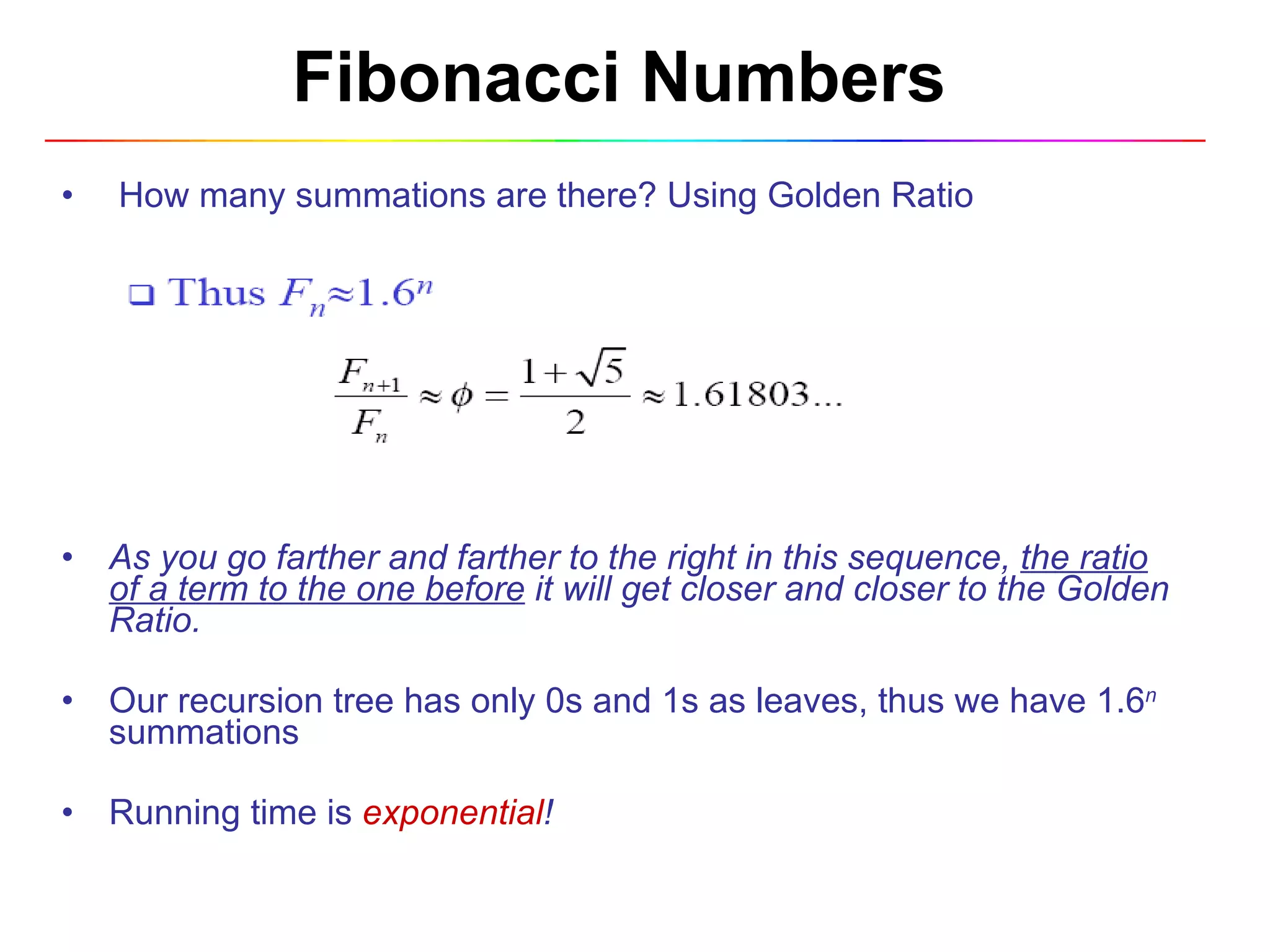
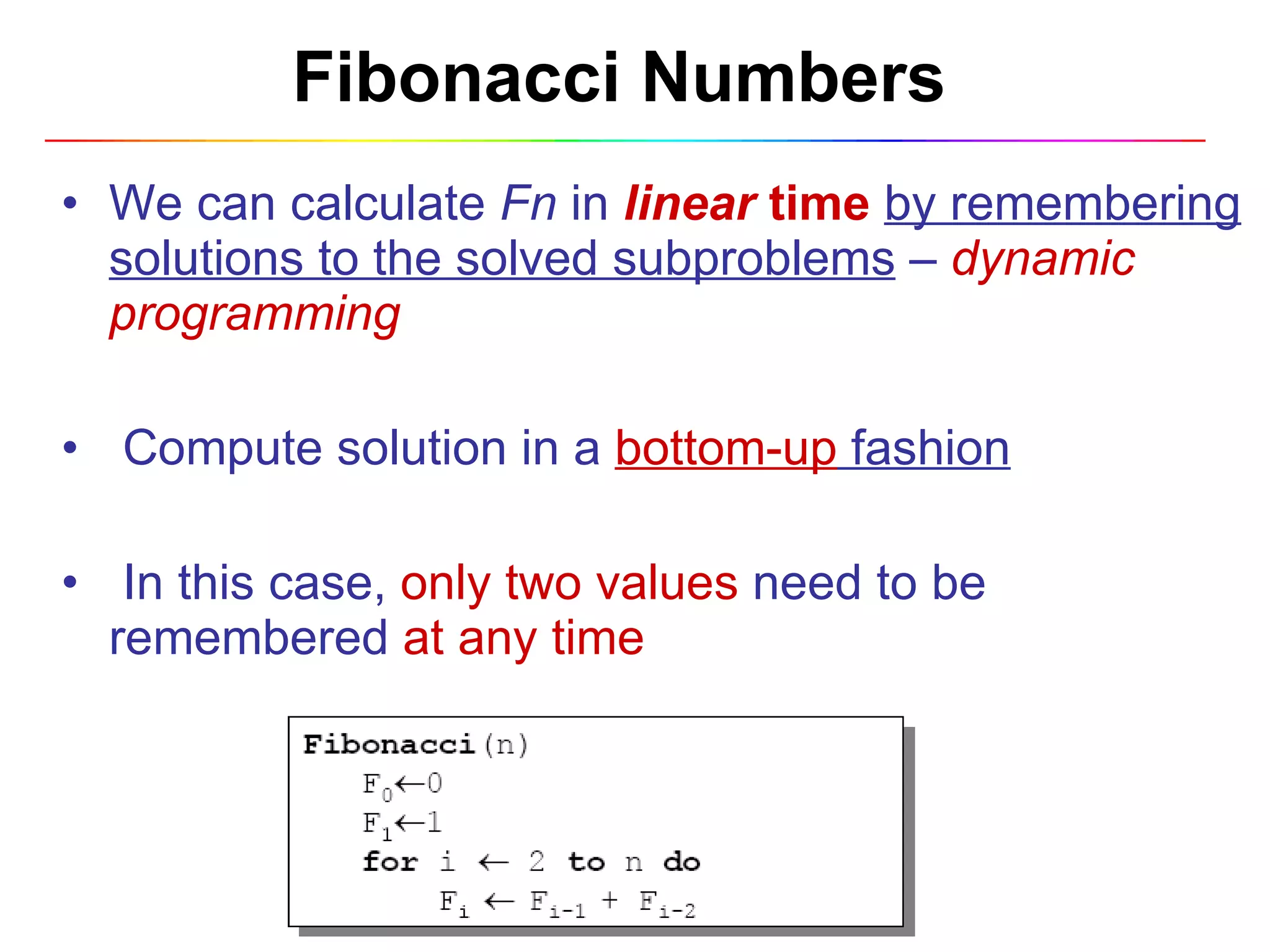
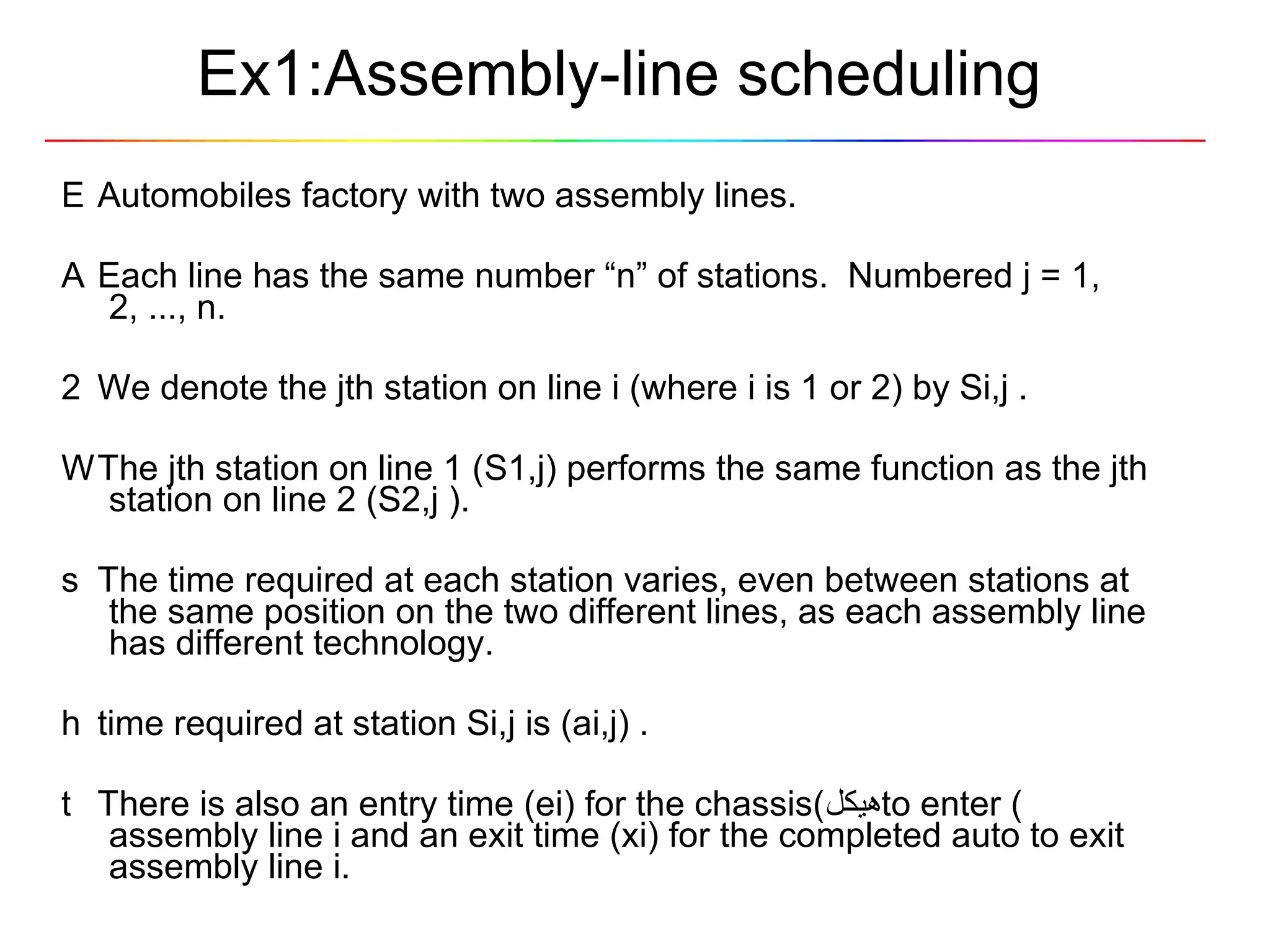
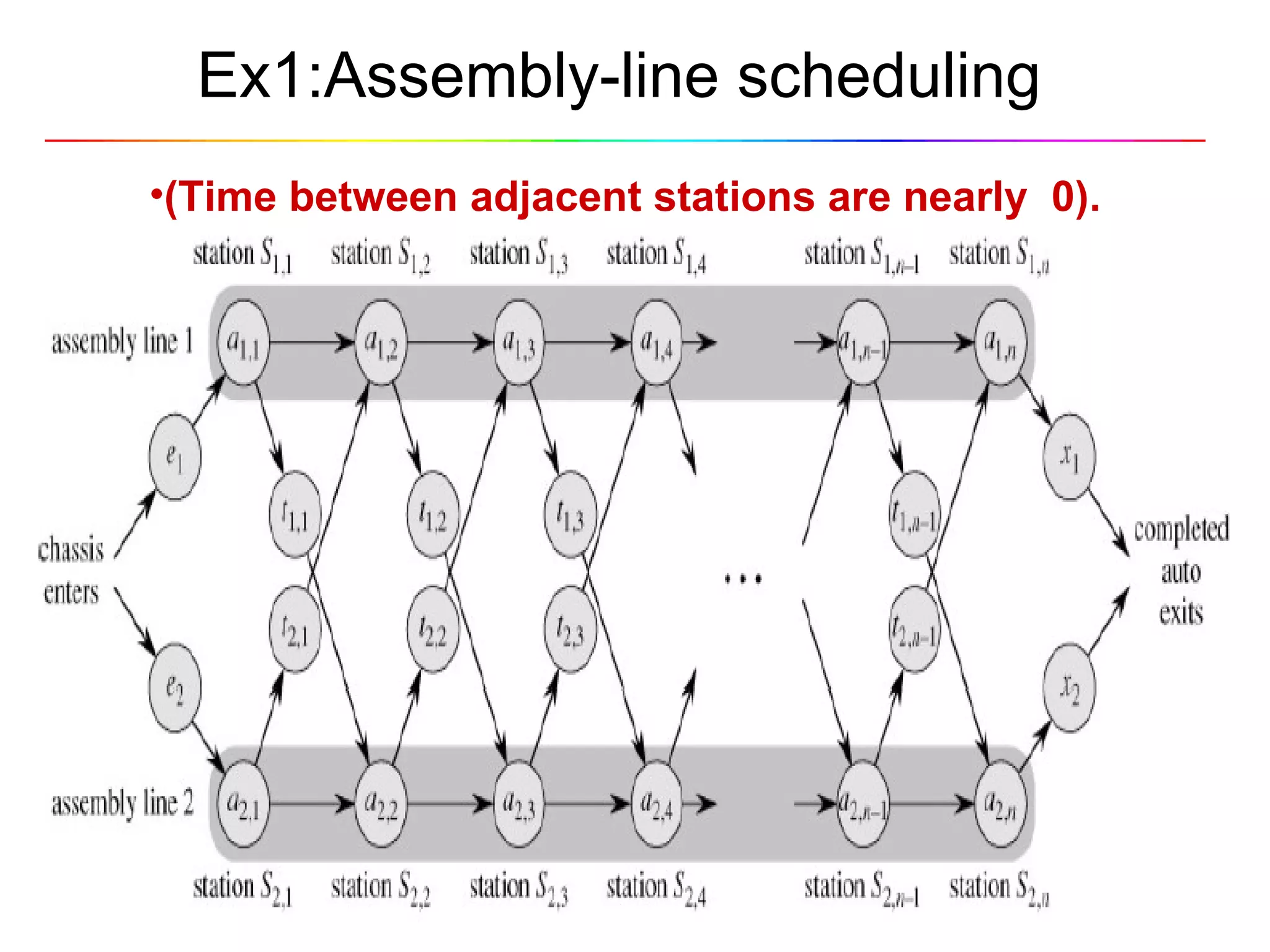
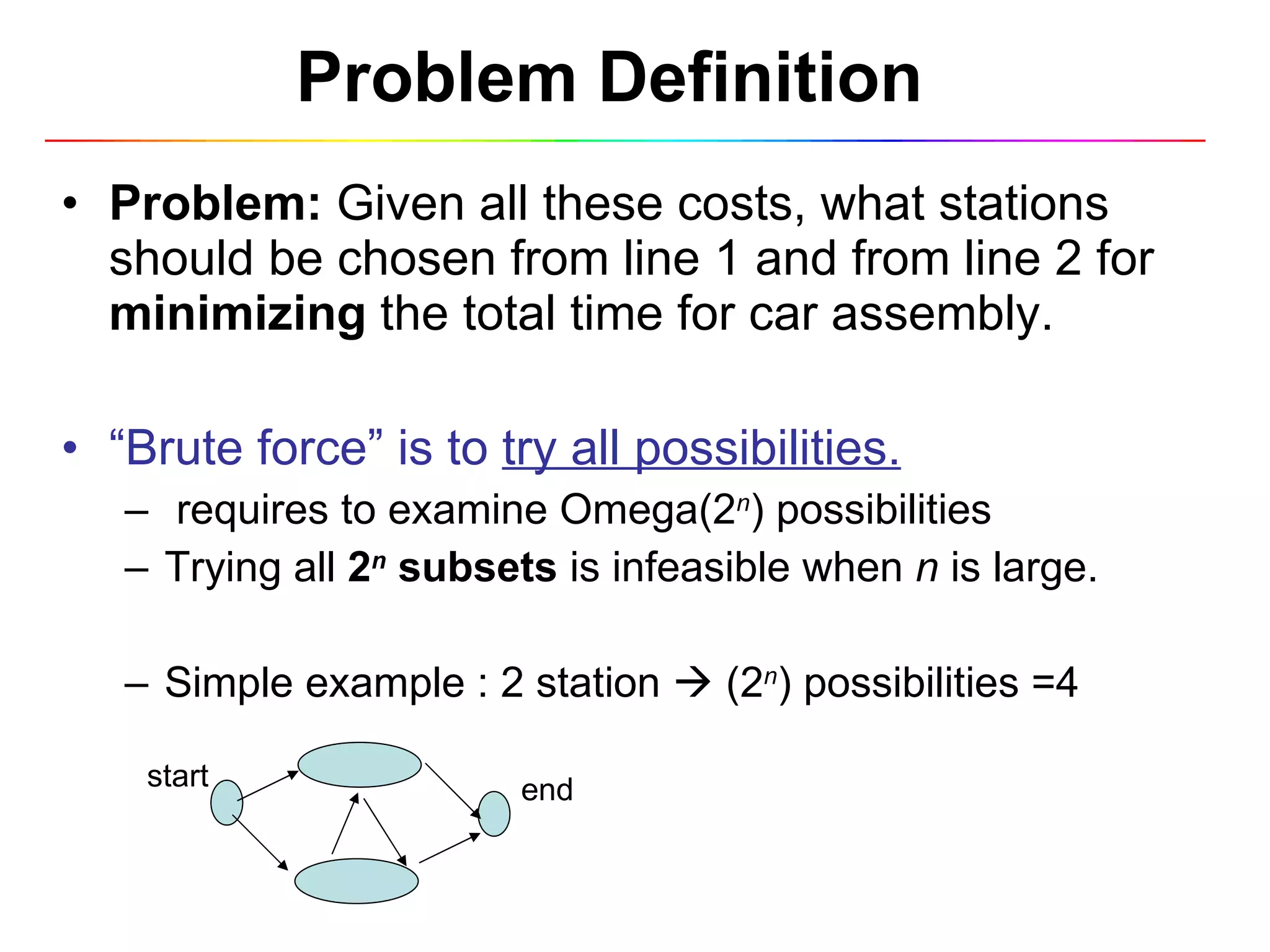
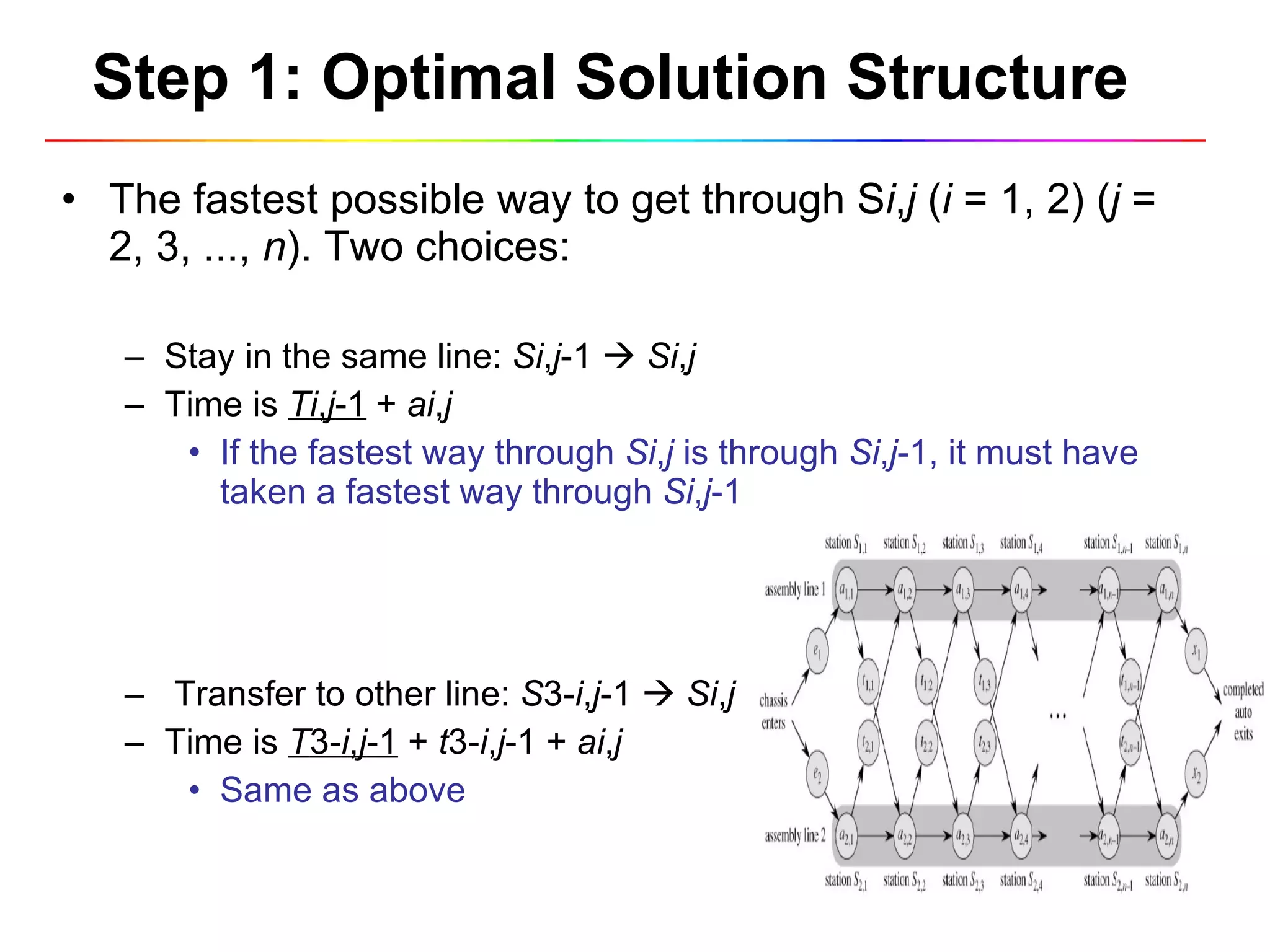
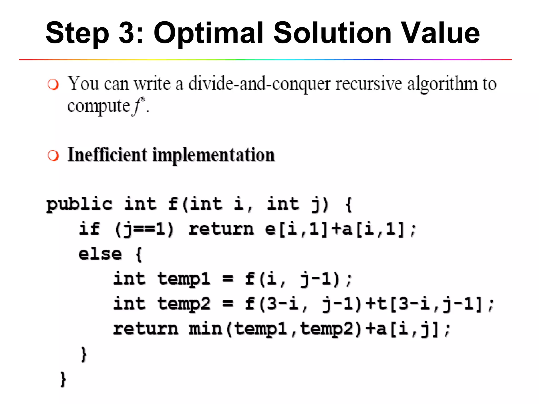
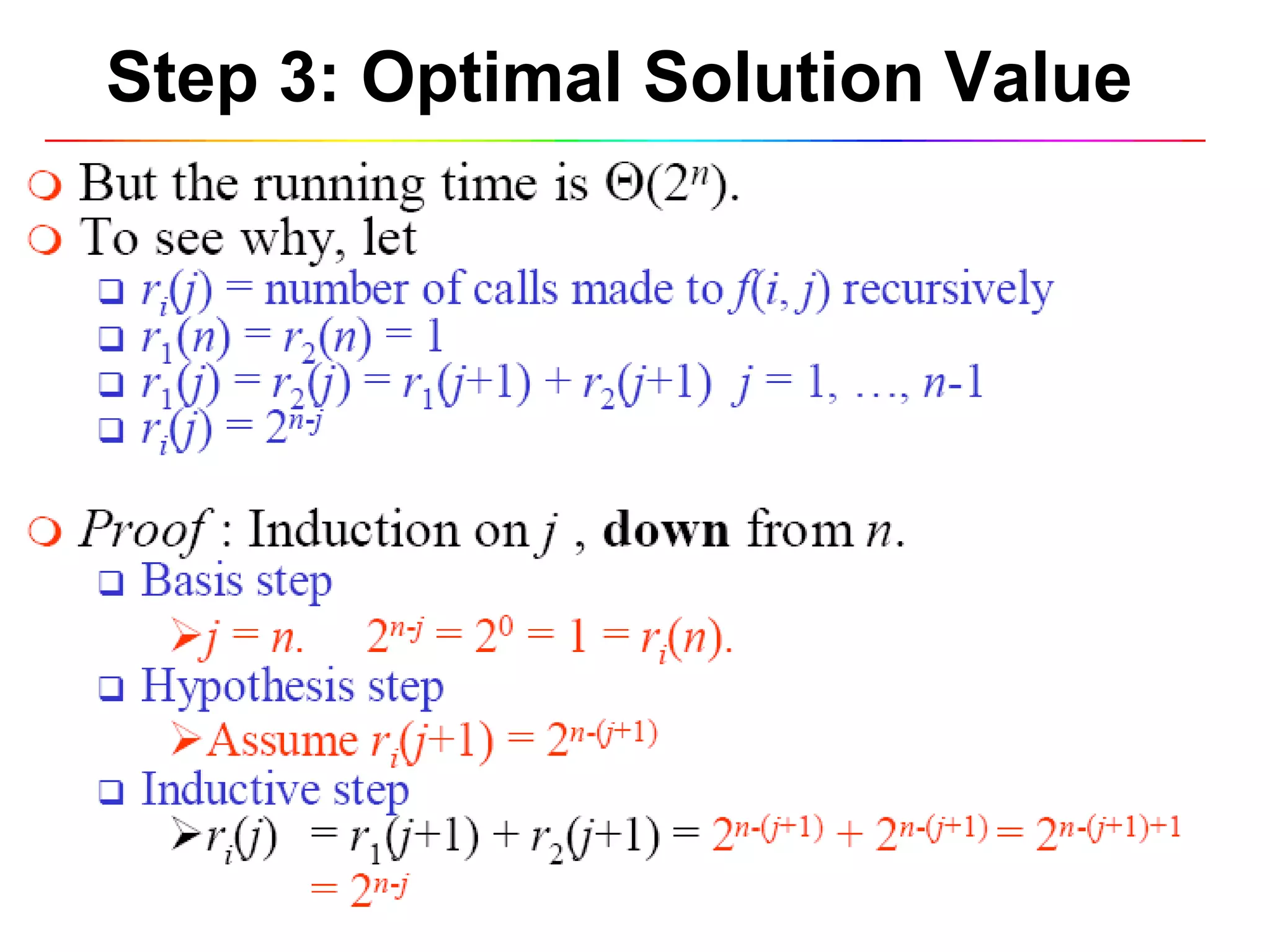
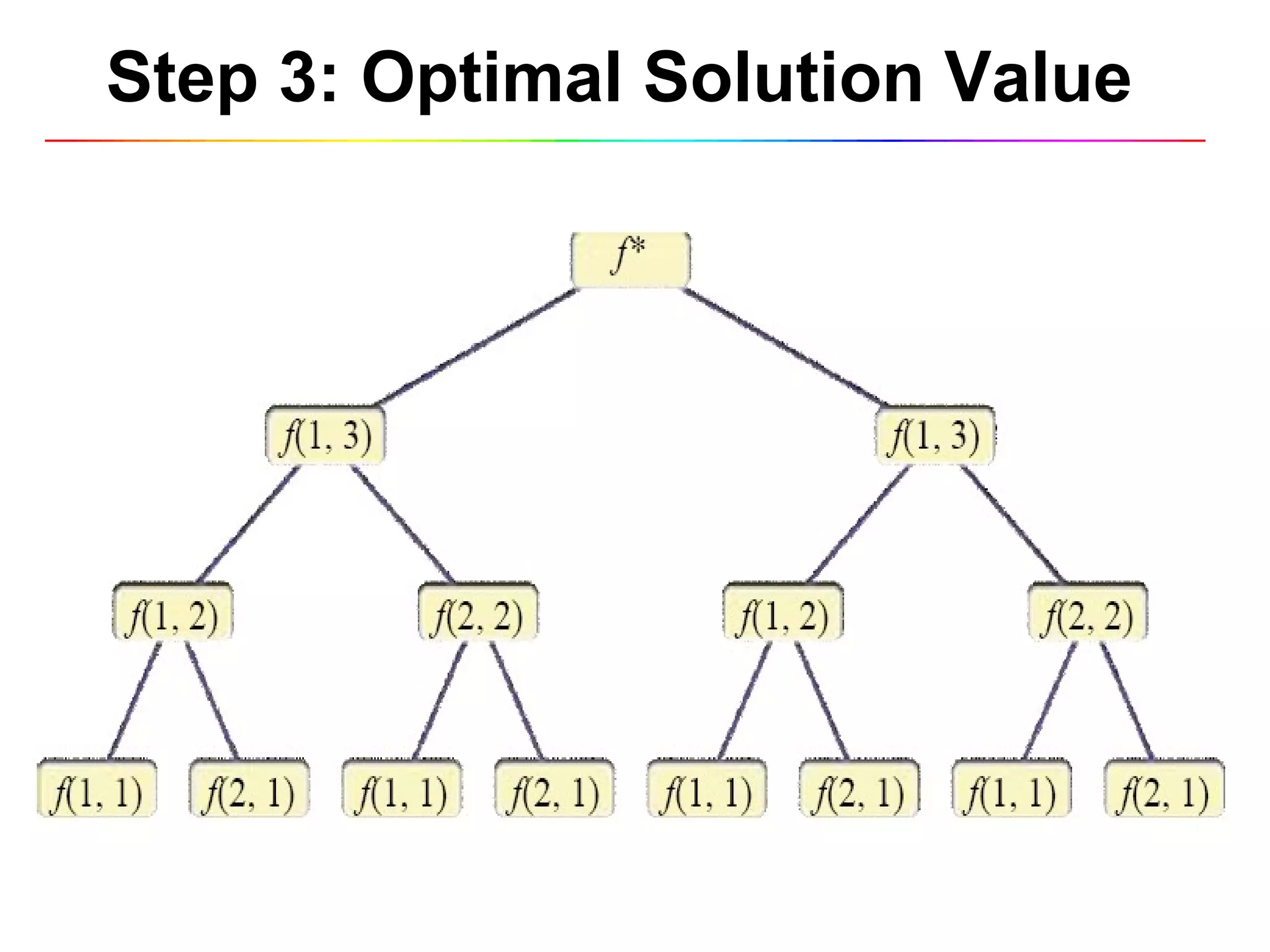
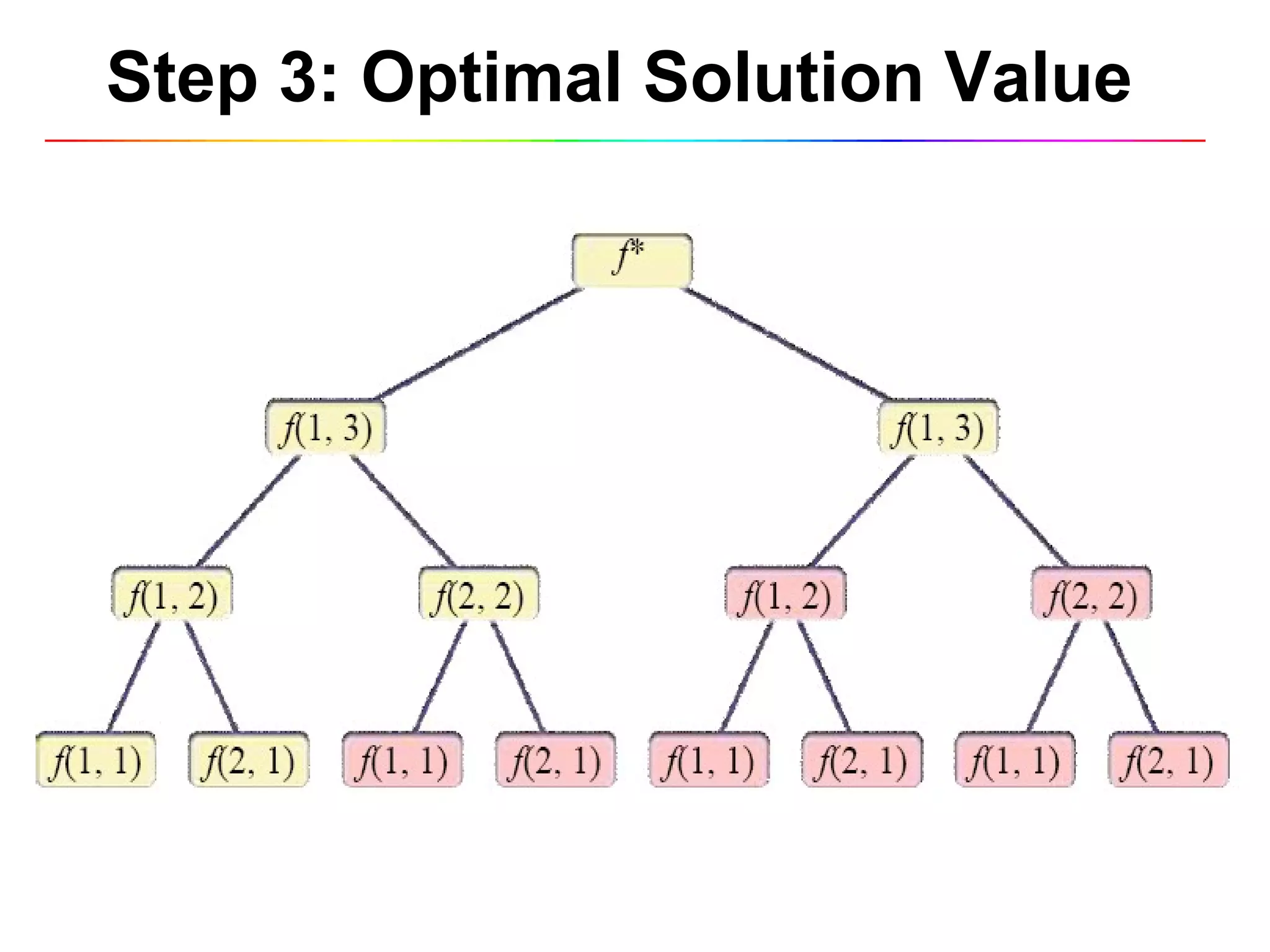
This document discusses algorithms for finding minimum and maximum elements in an array, including simultaneous minimum and maximum algorithms. It introduces dynamic programming as a technique for improving inefficient divide-and-conquer algorithms by storing results of subproblems to avoid recomputing them. Examples of dynamic programming include calculating the Fibonacci sequence and solving an assembly line scheduling problem to minimize total time.