Downloaded 3,789 times
![IMPORTANT DEFINITIONS IN L.P.
Solution:
A set of variables [X1,X2,...,Xn+m] is called a
solution to L.P. Problem if it satisfies its constraints.
Feasible Solution:
A set of variables [X1,X2,...,Xn+m] is called a
feasible solution to L.P. Problem if it satisfies its
constraints as well as non-negativity restrictions.
Optimal Feasible Solution:
The basic feasible solution that optimises the
objective function.
Unbounded Solution:
If the value of the objective function can be
increased or decreased indefinitely, the solution is called
an unbounded solution.](https://image.slidesharecdn.com/linearprograming-111120091922-phpapp02/75/Linear-programing-13-2048.jpg)


![IMPORTANT DEFINITIONS IN L.P.
Solution:
A set of variables [X1,X2,...,Xn+m] is called a
solution to L.P. Problem if it satisfies its constraints.
Feasible Solution:
A set of variables [X1,X2,...,Xn+m] is called a
feasible solution to L.P. Problem if it satisfies its
constraints as well as non-negativity restrictions.
Optimal Feasible Solution:
The basic feasible solution that optimises the
objective function.
Unbounded Solution:
If the value of the objective function can be
increased or decreased indefinitely, the solution is called
an unbounded solution.](https://crownmelresort.com/image.slidesharecdn.com/linearprograming-111120091922-phpapp02/75/Linear-programing-13-2048.jpg)


The document discusses linear programming (LP) as a mathematical method used for optimal resource allocation in various fields. It covers definitions, applications, advantages, limitations, and types of solutions in LP, alongside specific terminologies like feasible and optimal solutions. Additionally, it touches on duality and sensitivity analysis, which help in understanding the optimization process under varying conditions.
Presentation by Sankheerth P. and team introduces Linear Programming (LP) and its significance.
LP optimizes limited resources through mathematical modeling to find the best outcomes.
Describes essential requirements and assumptions for LP, such as defined objectives and resource limitations.
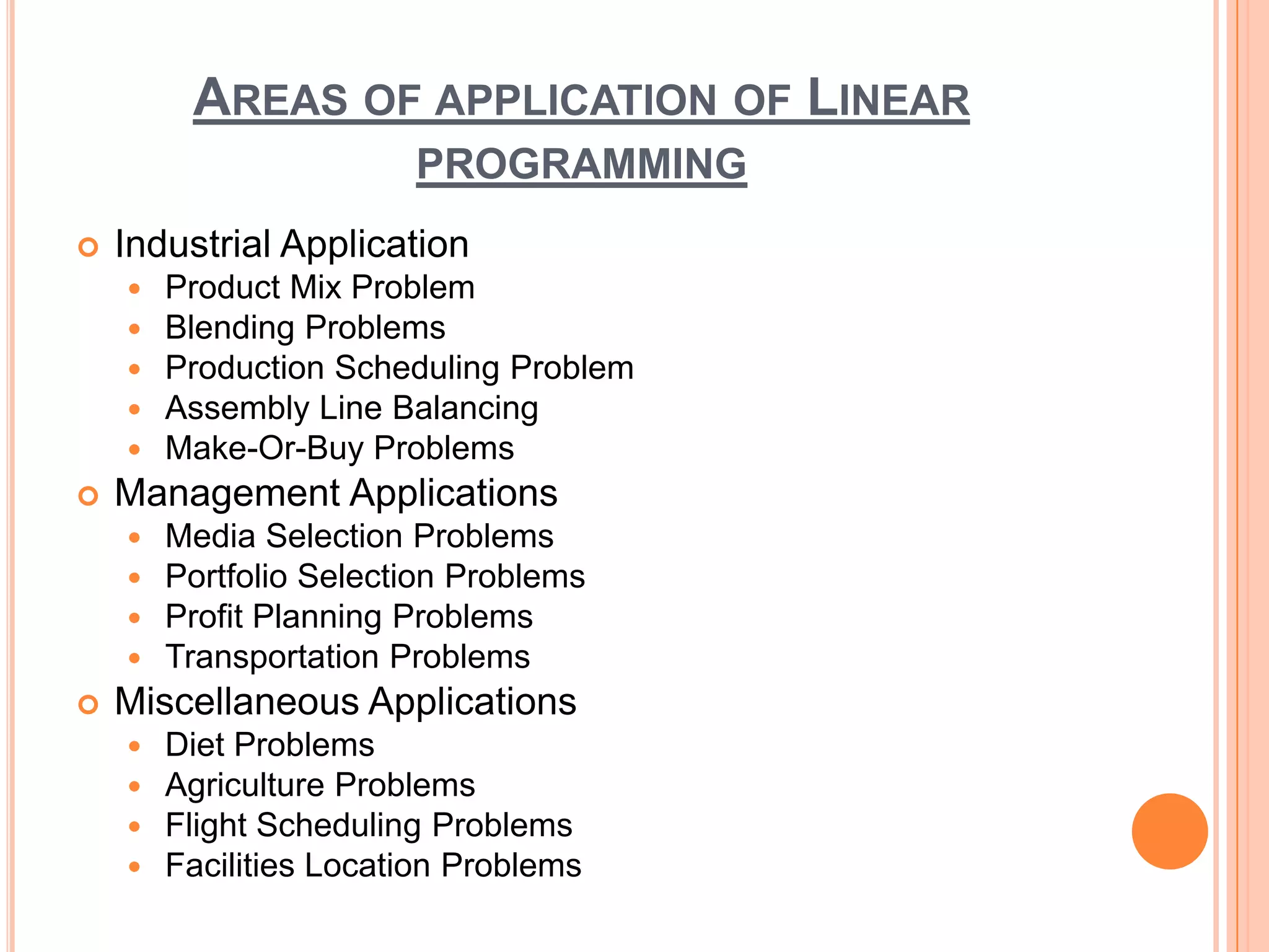
LP is utilized in diverse fields like business, industrial settings, military, and agriculture for optimizing processes.
LP aids in effective decision making and resource optimization but has limitations like computational difficulties and static applicability.
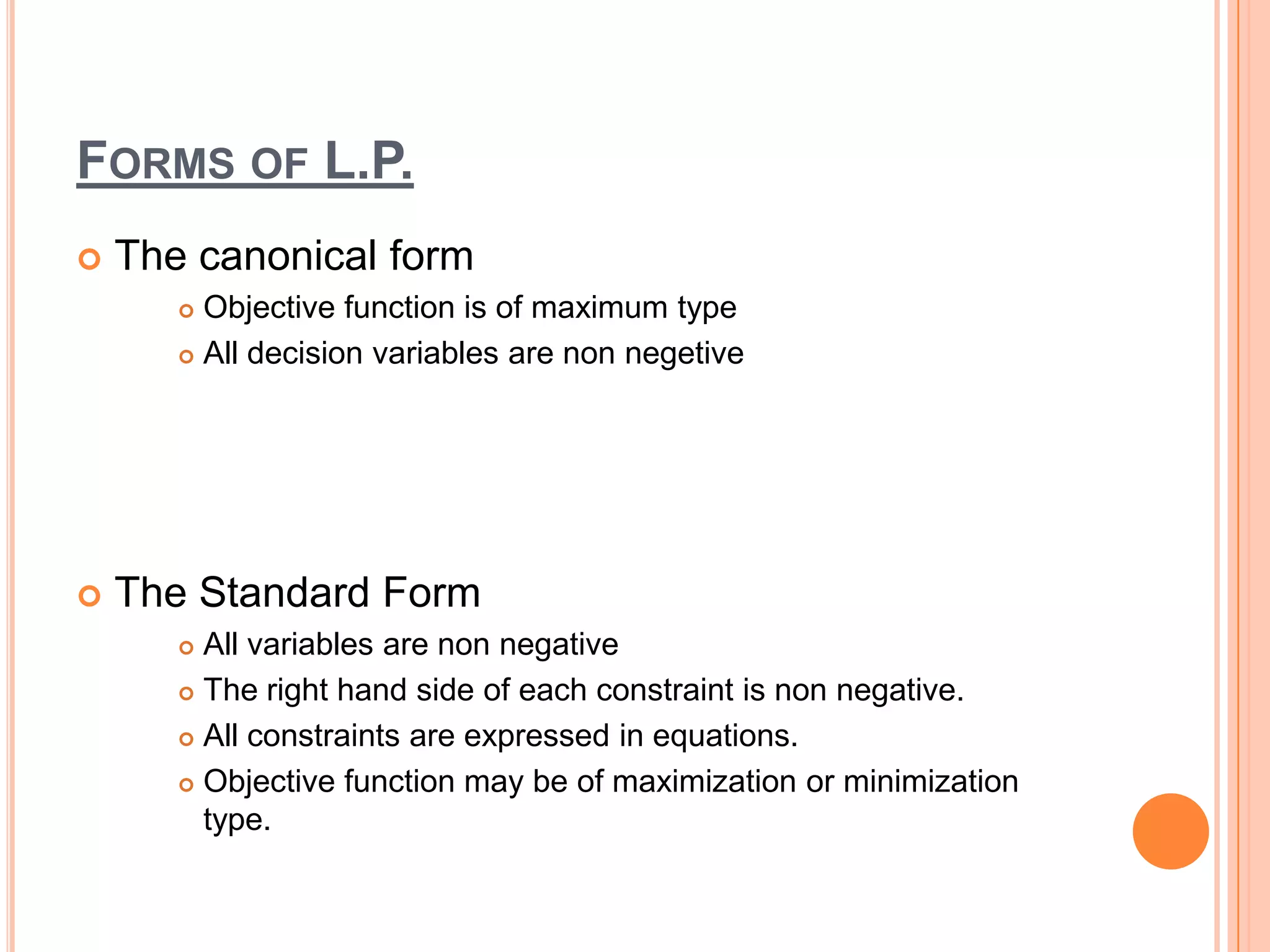
Discusses the graphical and simplex methods for solving LP along with forms of LP, including canonical and standard forms.
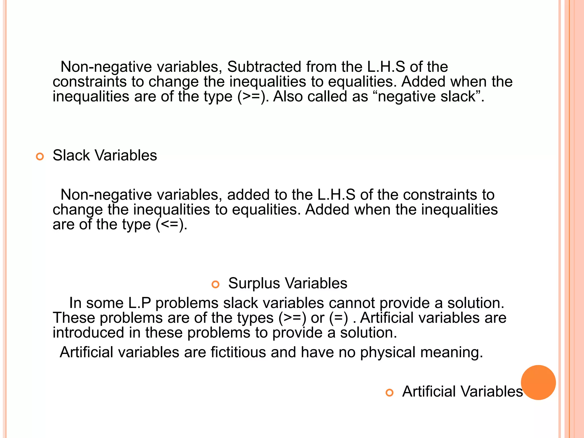
Key terms important in LP problems such as solution types, constraints, and variables like slack and artificial variables.
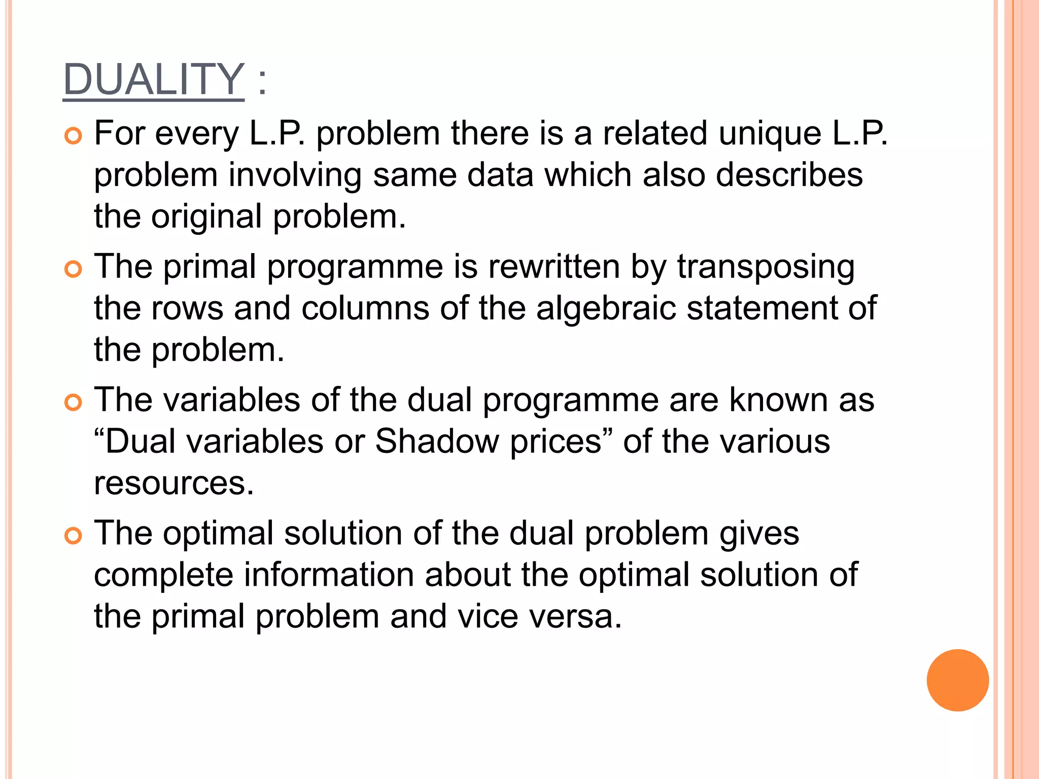
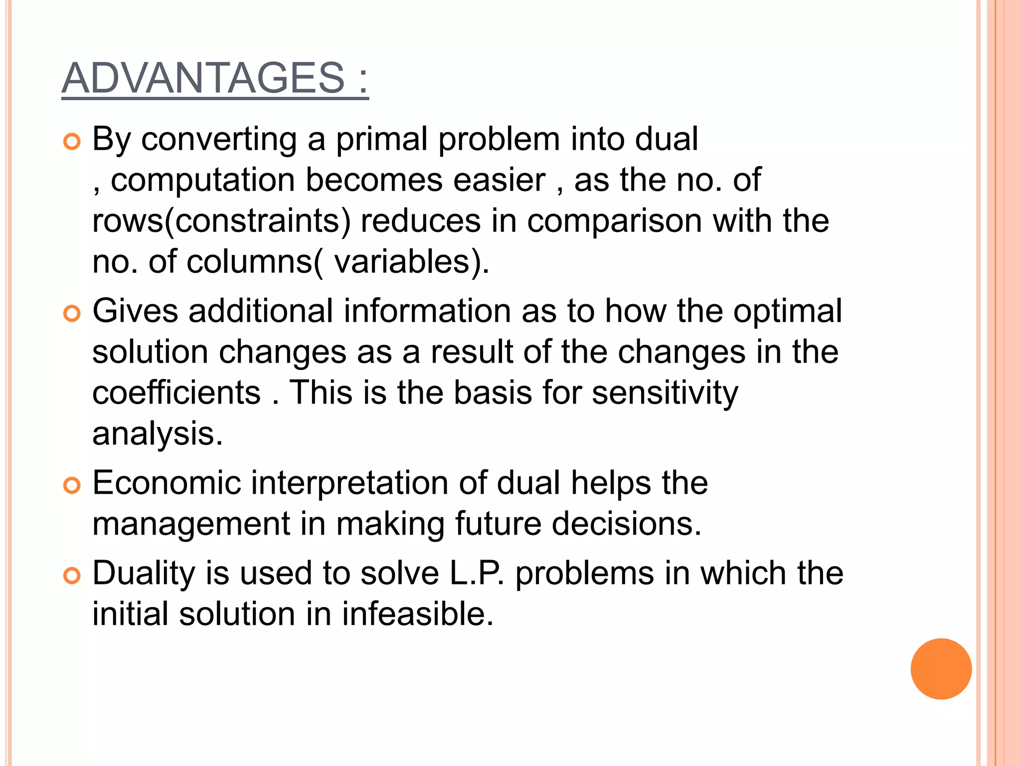
Explains the concept of duality in LP, emphasizing dual variables and the advantages of dual problem perspective in decision making.
Discusses post-optimality testing and how changing parameters affect optimal solutions through sensitivity analysis.
The presentation concludes with gratitude for the audience's attention and engagement.