The document discusses algorithm analysis and asymptotic notation. It defines algorithm analysis as comparing algorithms based on running time and other factors as problem size increases. Asymptotic notation such as Big-O, Big-Omega, and Big-Theta are introduced to classify algorithms based on how their running times grow relative to input size. Common time complexities like constant, logarithmic, linear, quadratic, and exponential are also covered. The properties and uses of asymptotic notation for equations and inequalities are explained.
To evaluate algorithms based on running time and other factors such as memory and effort. Running time analysis focuses on how it varies with problem size.
Describes worst-case (upper bound), best-case (lower bound), and average-case (predictive) running times for algorithms.
To compare algorithms, express running time as a function of input size and analyze functions asymptotically without machine dependency.
Asymptotic notation helps describe function behavior in limits, especially for worst-case running time functions.
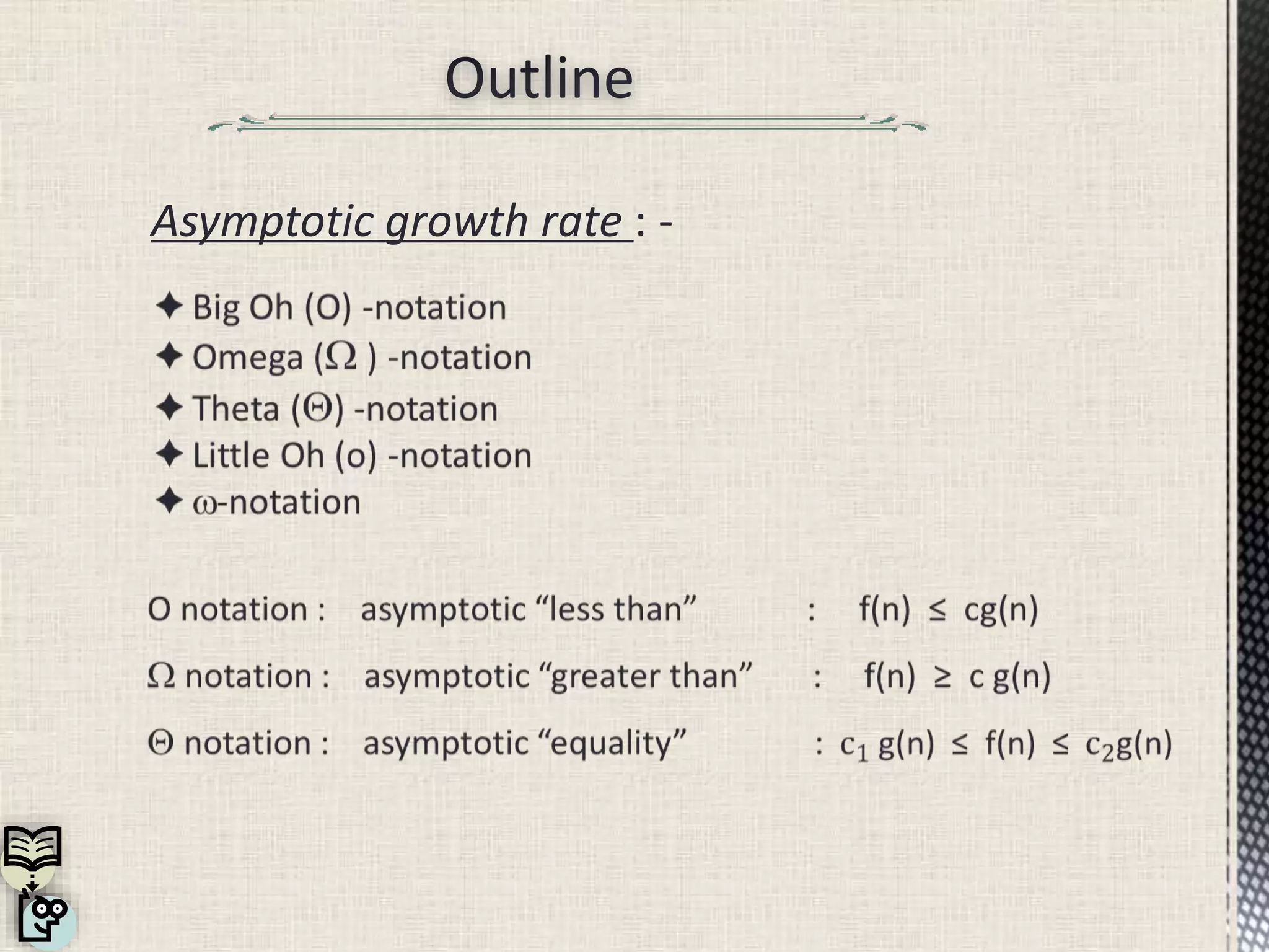
Asymptotic growth rates are defined, with Big-O notation indicating upper bounds on growth rate and conditions for it.
Demonstrates how to apply Big-O notation by comparing 2n² and n³, with methodical proofs for bounds.
Defines Big Omega as a lower bound and provides an example to illustrate how to determine the lower bound for functions.
Describes Big Theta as an asymptotic tight bound and gives an example of determining constants for a specific function.
Explains the relationship between Θ, O, and W notations, reinforcing that tight bounds connect upper and lower bounds.
Defines Little-o as a non-tight upper bound and gives criteria for when a function fits this notation.
Defines Little-ω as a non-tight lower bound with conditions for functions to fall into this category.
Analogies between various asymptotic notations and corresponding relationships between functions.
Various limits indicating the asymptotic behavior of functions and their classifications based on limits.
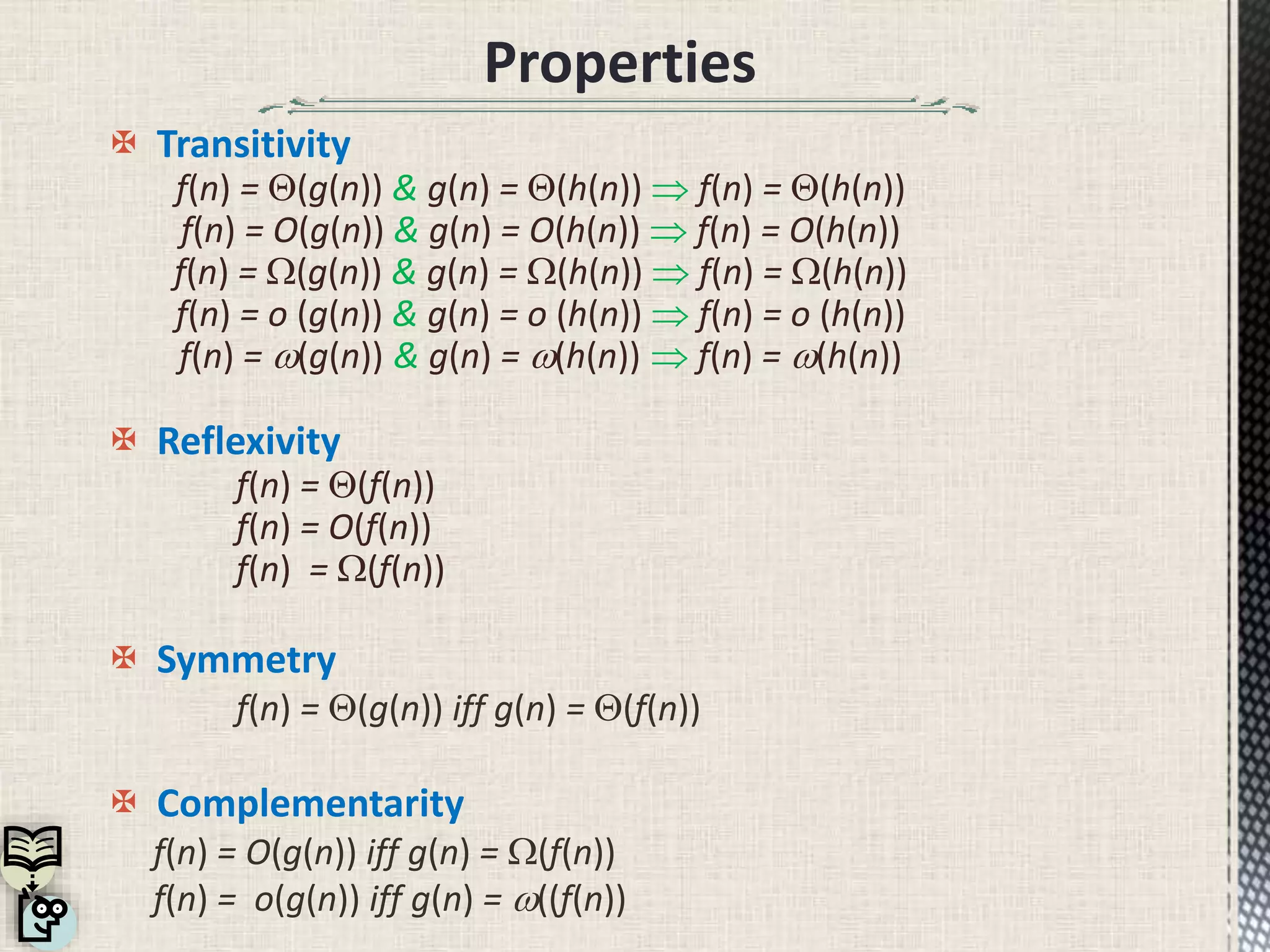
Discusses properties of transitivity, reflexivity, symmetry, and complementarity for asymptotic notations.
Shows how asymptotic notations can be applied in equations and the significance of anonymous functions.
Lists different complexity classes, including constant, logarithmic, linear, quadratic, and exponential complexities.
Thanks individuals who contributed to the project, emphasizing collaboration and support throughout the work.
What isthe goal of analysis of algorithms?
― To compare algorithms mainly in terms of running time but
also in terms of other factors (e.g., memory requirements,
programmer's effort etc.)
What do we mean by running time analysis?
― Determine how running time increases as the size of the
problem increases.
An algorithm is a finite set of precise instructions for
performing a computation or for solving a problem.
3.
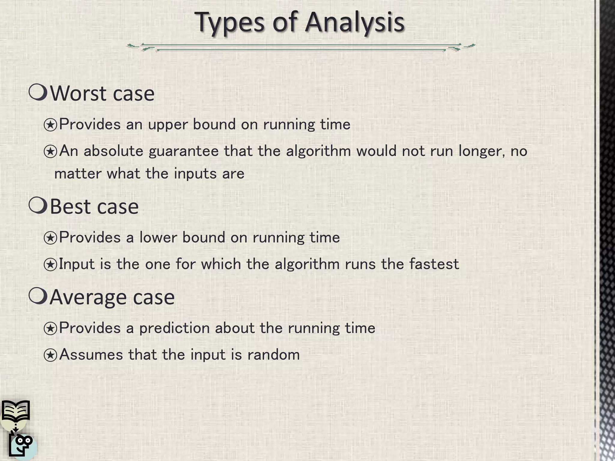
Worst case
⍟Provides anupper bound on running time
⍟An absolute guarantee that the algorithm would not run longer, no
matter what the inputs are
Best case
⍟Provides a lower bound on running time
⍟Input is the one for which the algorithm runs the fastest
Average case
⍟Provides a prediction about the running time
⍟Assumes that the input is random
4.
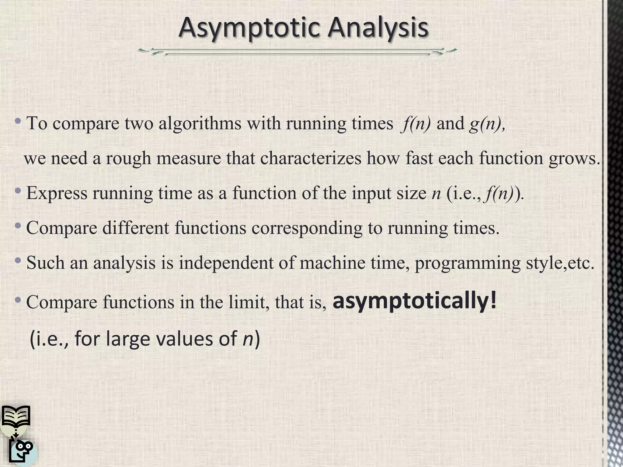
• To comparetwo algorithms with running times f(n) and g(n),
we need a rough measure that characterizes how fast each function grows.
• Express running time as a function of the input size n (i.e., f(n)).
• Compare different functions corresponding to running times.
• Such an analysis is independent of machine time, programming style,etc.
• Compare functions in the limit, that is, asymptotically!
(i.e., for large values of n)
5.
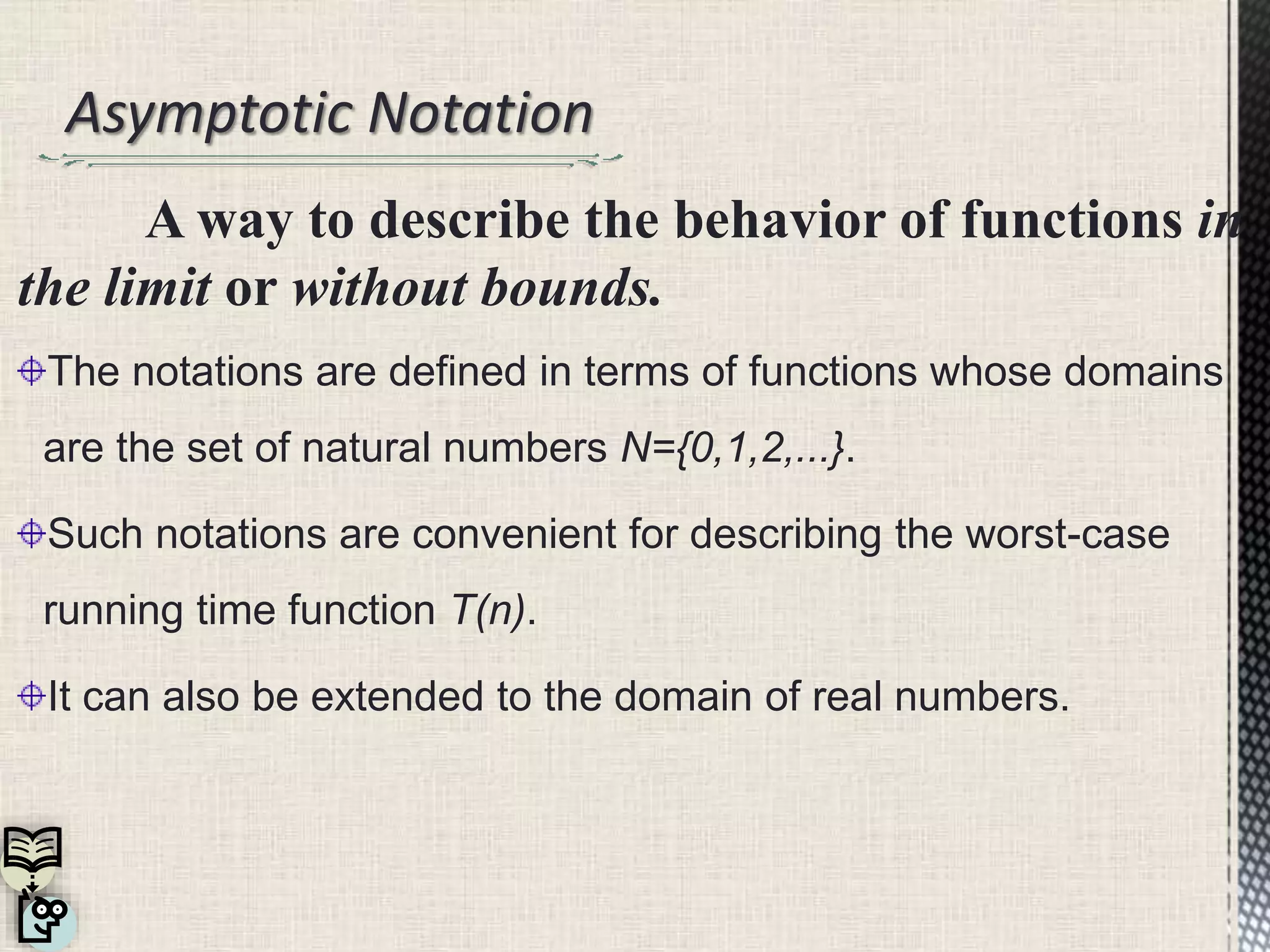
Asymptotic Notation
A wayto describe the behavior of functions in
the limit or without bounds.
The notations are defined in terms of functions whose domains
are the set of natural numbers N={0,1,2,...}.
Such notations are convenient for describing the worst-case
running time function T(n).
It can also be extended to the domain of real numbers.
6.
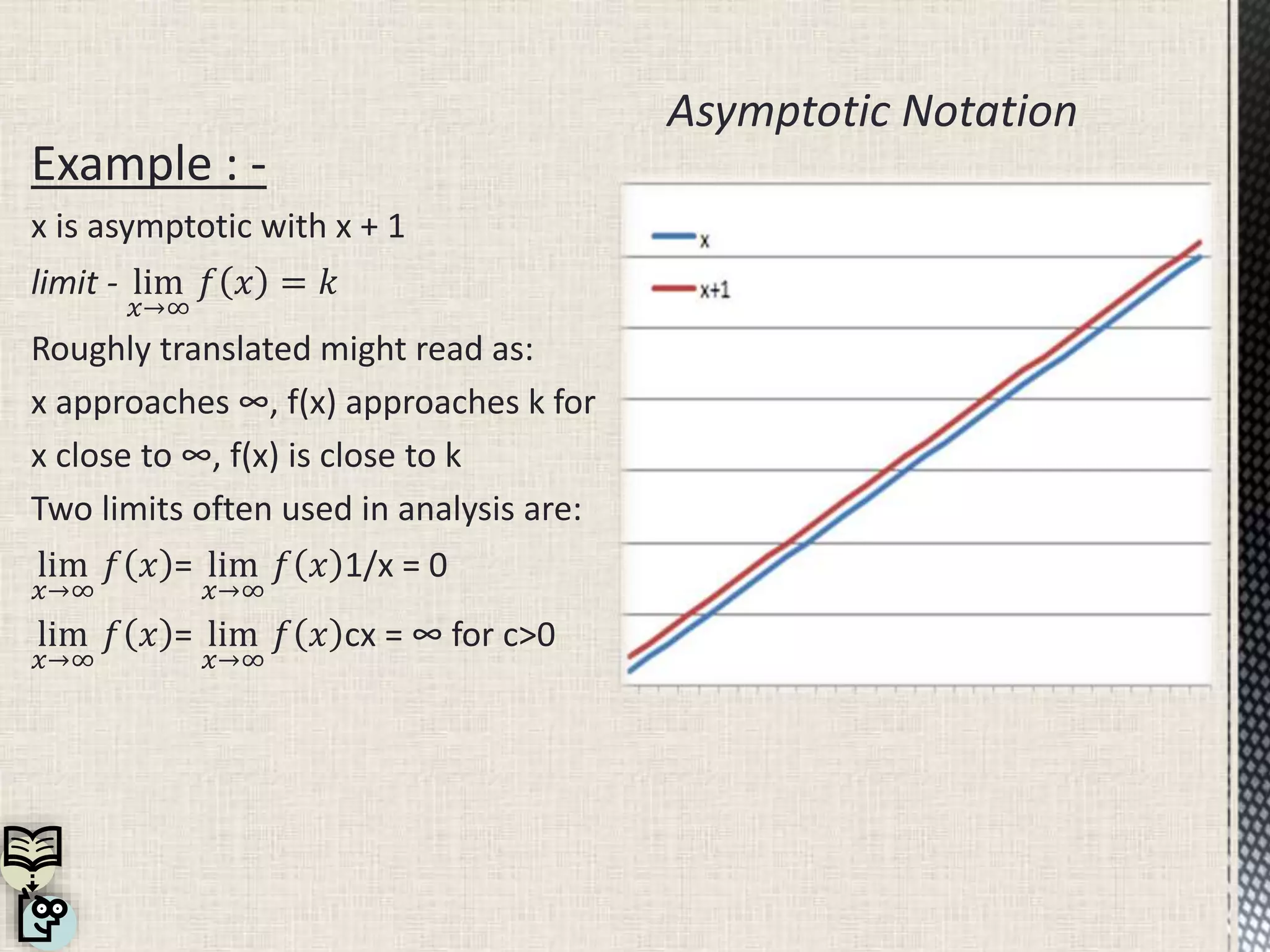
Example : -
xis asymptotic with x + 1
limit - lim
𝑥→∞
𝑓 𝑥 = 𝑘
Roughly translated might read as:
x approaches ∞, f(x) approaches k for
x close to ∞, f(x) is close to k
Two limits often used in analysis are:
lim
𝑥→∞
𝑓 𝑥 = lim
𝑥→∞
𝑓 𝑥 1/x = 0
lim
𝑥→∞
𝑓 𝑥 = lim
𝑥→∞
𝑓 𝑥 cx = ∞ for c>0
Asymptotic Notation
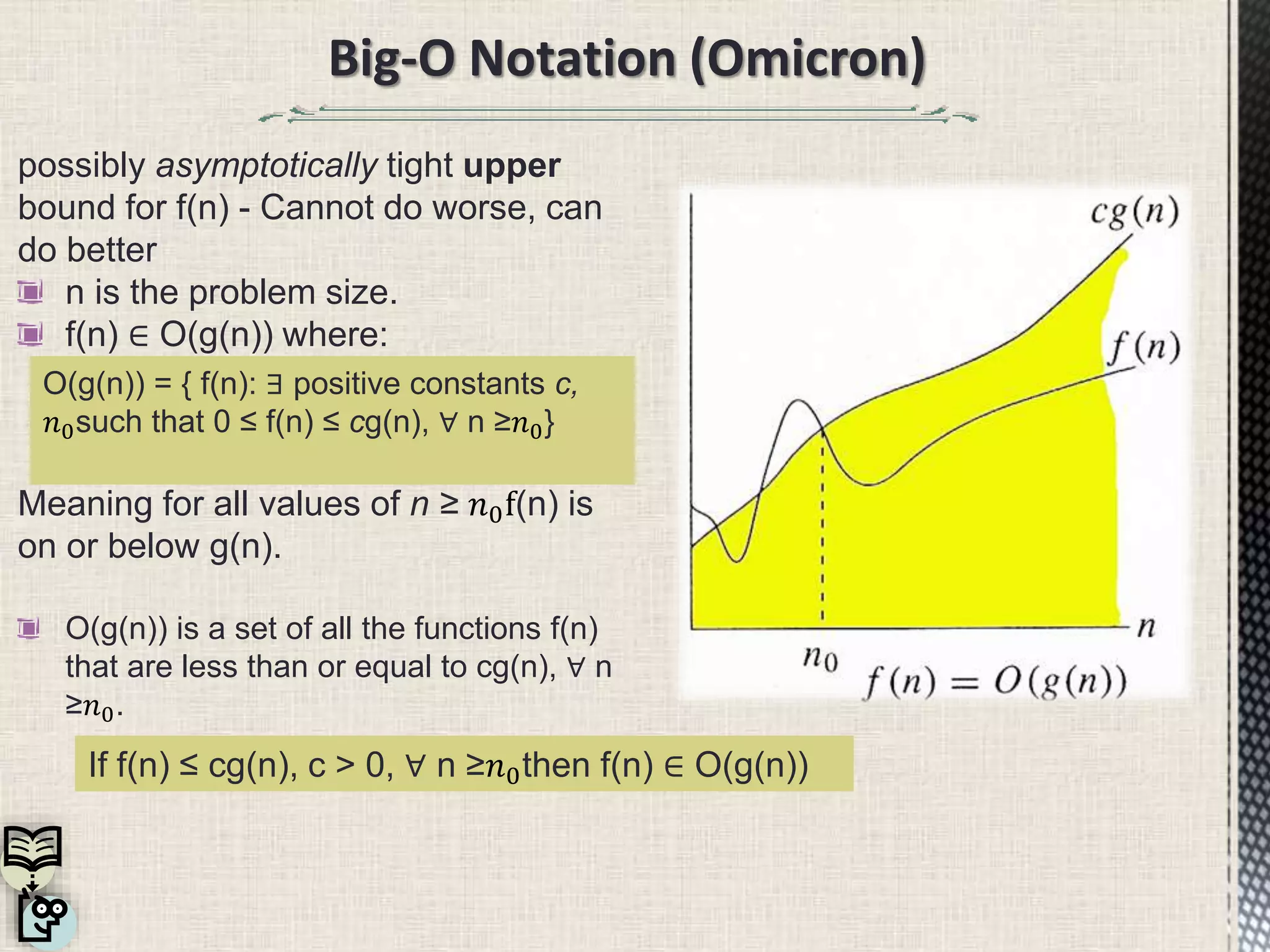
possibly asymptotically tightupper
bound for f(n) - Cannot do worse, can
do better
n is the problem size.
f(n) ∈ O(g(n)) where:
Meaning for all values of n ≥ 𝑛0f(n) is
on or below g(n).
O(g(n)) is a set of all the functions f(n)
that are less than or equal to cg(n), ∀ n
≥𝑛0.
Big-O Notation (Omicron)
O(g(n)) = { f(n): ∃ positive constants c,
𝑛0such that 0 ≤ f(n) ≤ cg(n), ∀ n ≥𝑛0}
If f(n) ≤ cg(n), c > 0, ∀ n ≥𝑛0then f(n) ∈ O(g(n))
9.
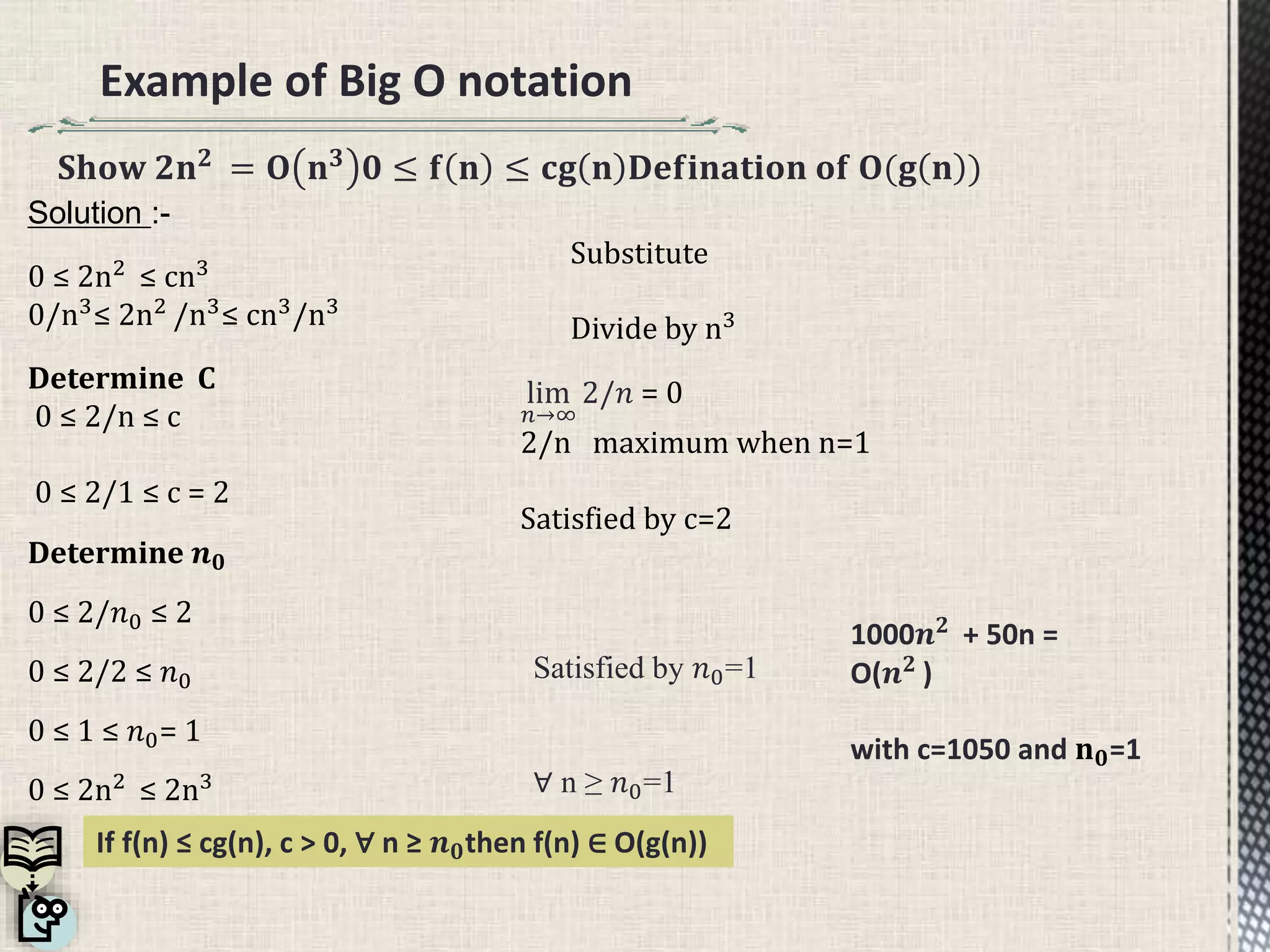
Example of BigO notation
𝐒𝐡𝐨𝐰 𝟐𝐧 𝟐 = 𝐎 𝐧 𝟑 𝟎 ≤ 𝐟 𝐧 ≤ 𝐜𝐠 𝐧 𝐃𝐞𝐟𝐢𝐧𝐚𝐭𝐢𝐨𝐧 𝐨𝐟 𝐎(𝐠 𝐧 )
Solution :-
0 ≤ 2n2
≤ cn3
0/n3≤ 2n2 /n3≤ cn3/n3
Determine C
0 ≤ 2/n ≤ c
0 ≤ 2/1 ≤ c = 2
Substitute
Divide by n3
lim
𝑛→∞
2/𝑛 = 0
2/n maximum when n=1
Satisfied by c=2
1000𝒏 𝟐 + 50n =
O(𝒏 𝟐
)
with c=1050 and 𝐧 𝟎=1
Satisfied by 𝑛0=1
∀ n ≥ 𝑛0=1
If f(n) ≤ cg(n), c > 0, ∀ n ≥ 𝒏 𝟎then f(n) ∈ O(g(n))
Determine 𝒏 𝟎
0 ≤ 2/𝑛0 ≤ 2
0 ≤ 2/2 ≤ 𝑛0
0 ≤ 1 ≤ 𝑛0= 1
0 ≤ 2n2
≤ 2n3
10.
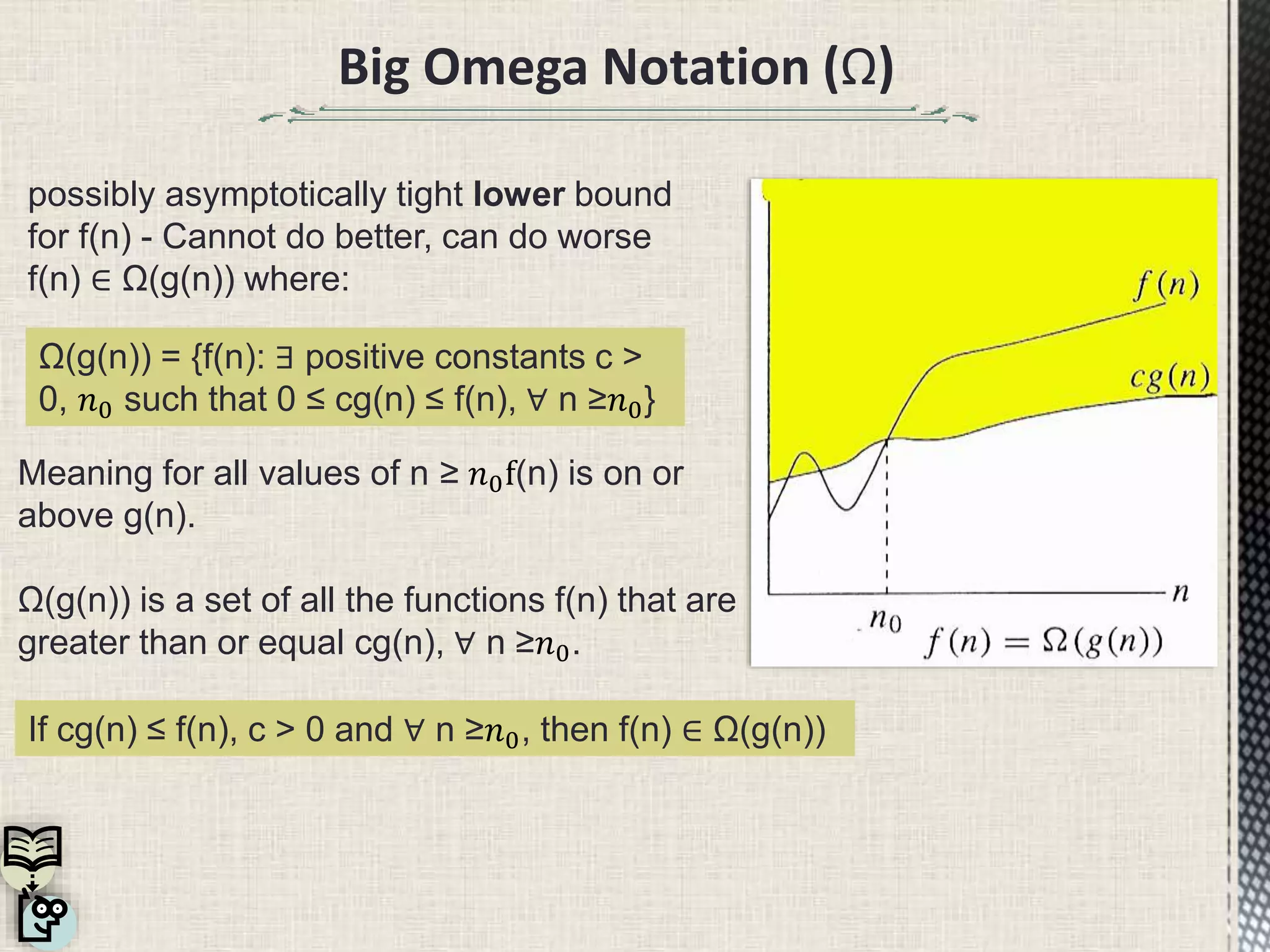
Big Omega Notation(Ω)
possibly asymptotically tight lower bound
for f(n) - Cannot do better, can do worse
f(n) ∈ Ω(g(n)) where:
Meaning for all values of n ≥ 𝑛0f(n) is on or
above g(n).
Ω(g(n)) is a set of all the functions f(n) that are
greater than or equal cg(n), ∀ n ≥𝑛0.
Ω(g(n)) = {f(n): ∃ positive constants c >
0, 𝑛0 such that 0 ≤ cg(n) ≤ f(n), ∀ n ≥𝑛0}
If cg(n) ≤ f(n), c > 0 and ∀ n ≥𝑛0, then f(n) ∈ Ω(g(n))
11.
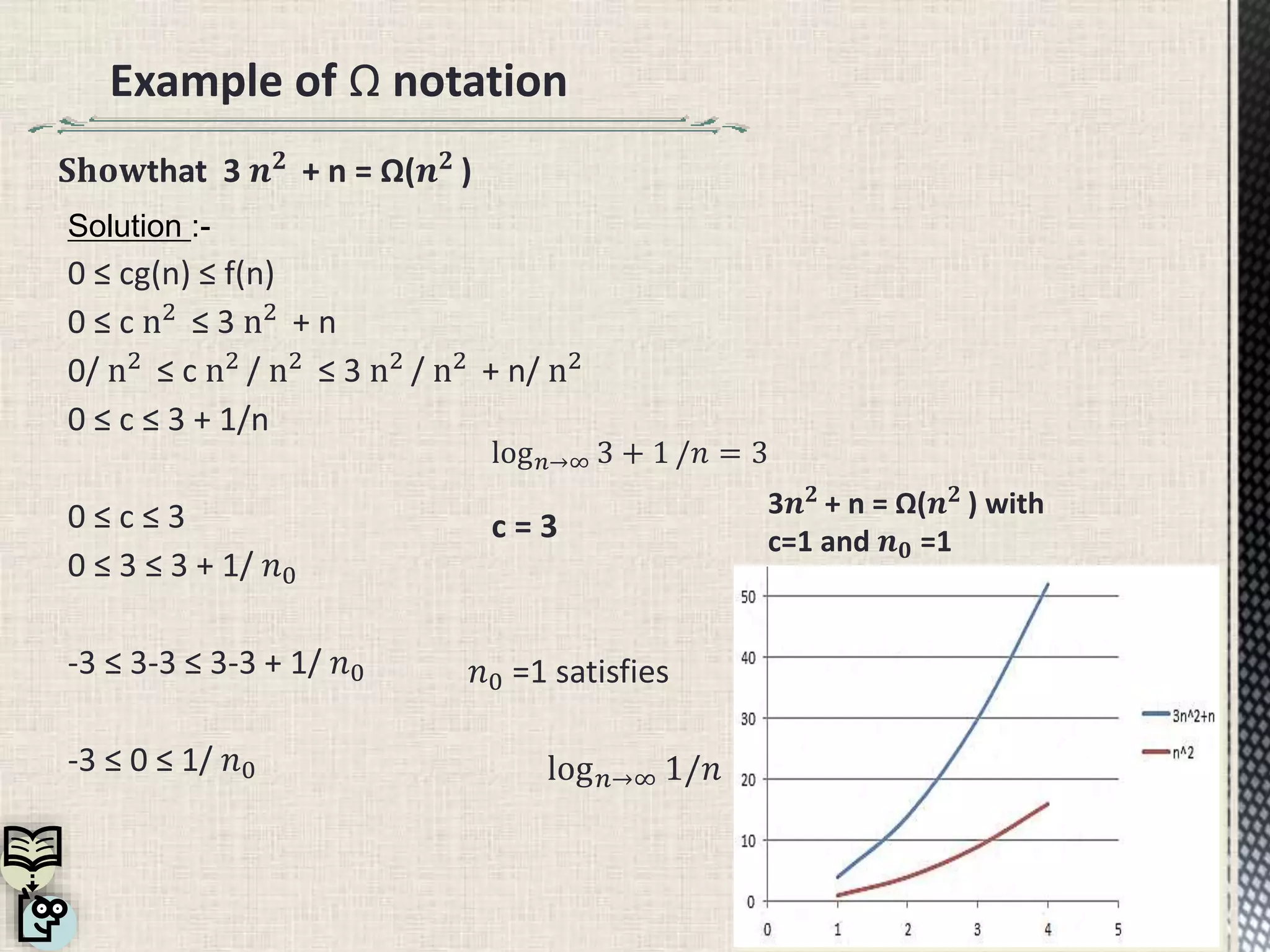
Example of Ωnotation
Solution :-
0 ≤ cg(n) ≤ f(n)
0 ≤ c n2 ≤ 3 n2 + n
0/ n2 ≤ c n2 / n2 ≤ 3 n2 / n2 + n/ n2
0 ≤ c ≤ 3 + 1/n
0 ≤ c ≤ 3
0 ≤ 3 ≤ 3 + 1/ 𝑛0
-3 ≤ 3-3 ≤ 3-3 + 1/ 𝑛0
-3 ≤ 0 ≤ 1/ 𝑛0
𝑛0 =1 satisfies
log 𝑛→∞ 1/𝑛
log 𝑛→∞ 3 + 1 /𝑛 = 3
c = 3
𝐒𝐡𝐨𝐰that 3 𝒏 𝟐
+ n = Ω(𝒏 𝟐
)
3𝒏 𝟐 + n = Ω(𝒏 𝟐 ) with
c=1 and 𝒏 𝟎 =1
12.
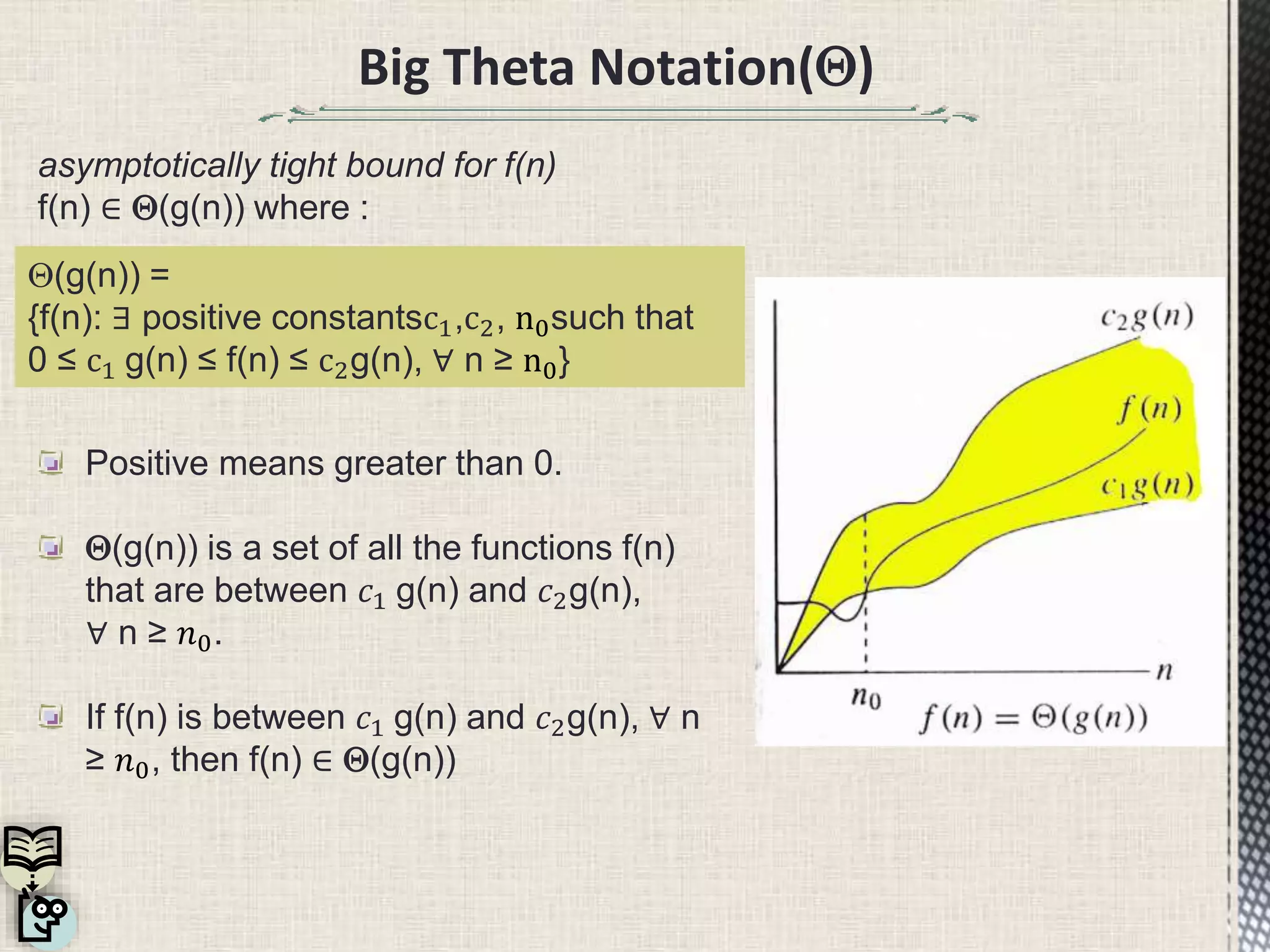
Big Theta Notation()
asymptoticallytight bound for f(n)
f(n) ∈ (g(n)) where :
Positive means greater than 0.
(g(n)) is a set of all the functions f(n)
that are between 𝑐1 g(n) and 𝑐2g(n),
∀ n ≥ 𝑛0.
If f(n) is between 𝑐1 g(n) and 𝑐2g(n), ∀ n
≥ 𝑛0, then f(n) ∈ (g(n))
(g(n)) =
{f(n): ∃ positive constantsc1,c2, n0such that
0 ≤ c1 g(n) ≤ f(n) ≤ c2g(n), ∀ n ≥ n0}
13.
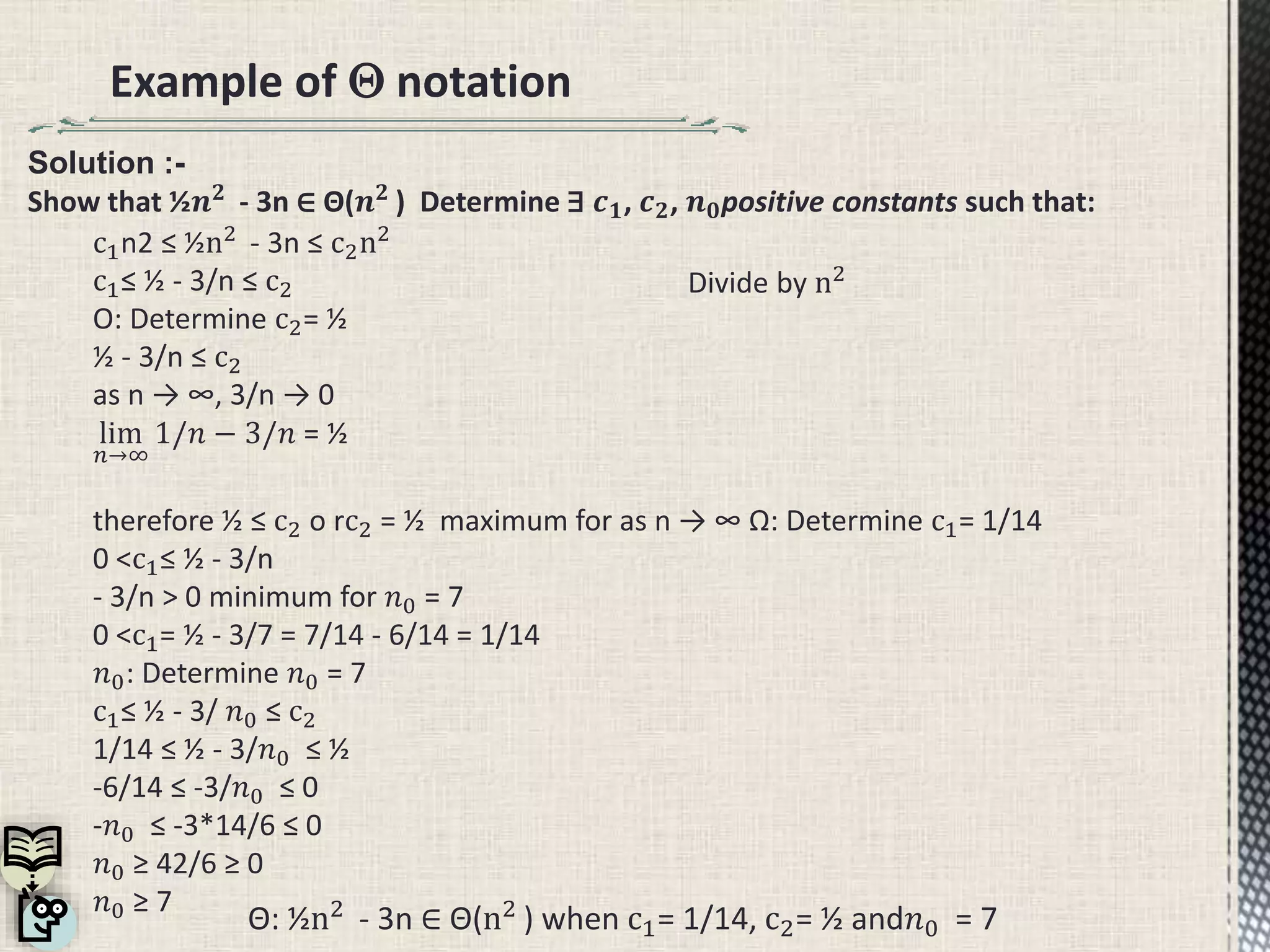
Example of notation
Θ: ½n2
- 3n ∈ Θ(n2
) when c1= 1/14, c2= ½ and𝑛0 = 7
Divide by n2
c1n2 ≤ ½n2
- 3n ≤ c2n2
c1≤ ½ - 3/n ≤ c2
O: Determine c2= ½
½ - 3/n ≤ c2
as n → ∞, 3/n → 0
lim
𝑛→∞
1/𝑛 − 3/𝑛 = ½
therefore ½ ≤ c2 o rc2 = ½ maximum for as n → ∞ Ω: Determine c1= 1/14
0 <c1≤ ½ - 3/n
- 3/n > 0 minimum for 𝑛0 = 7
0 <c1= ½ - 3/7 = 7/14 - 6/14 = 1/14
𝑛0: Determine 𝑛0 = 7
c1≤ ½ - 3/ 𝑛0 ≤ c2
1/14 ≤ ½ - 3/𝑛0 ≤ ½
-6/14 ≤ -3/𝑛0 ≤ 0
-𝑛0 ≤ -3*14/6 ≤ 0
𝑛0 ≥ 42/6 ≥ 0
𝑛0 ≥ 7
Solution :-
Show that ½𝒏 𝟐
- 3n ∈ Θ(𝒏 𝟐
) Determine ∃ 𝒄 𝟏, 𝒄 𝟐, 𝒏 𝟎positive constants such that:
14.
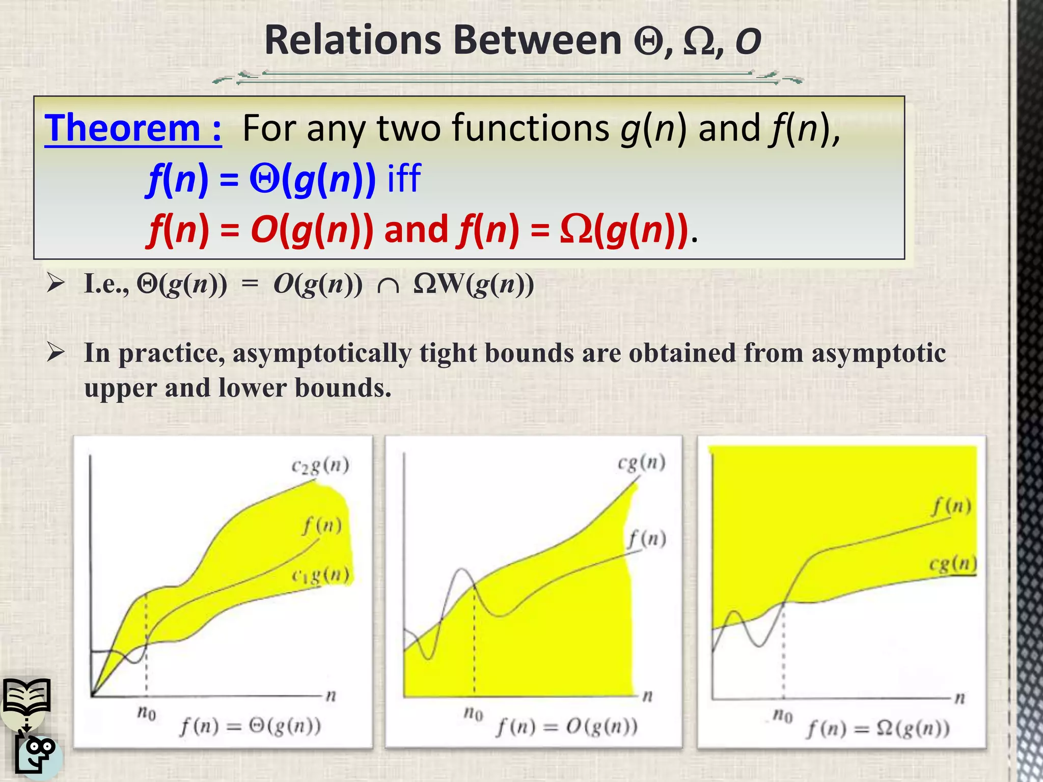
Relations Between ,W, O
Theorem : For any two functions g(n) and f(n),
f(n) = (g(n)) iff
f(n) = O(g(n)) and f(n) = W(g(n)).
I.e., (g(n)) = O(g(n)) WW(g(n))
In practice, asymptotically tight bounds are obtained from asymptotic
upper and lower bounds.
15.
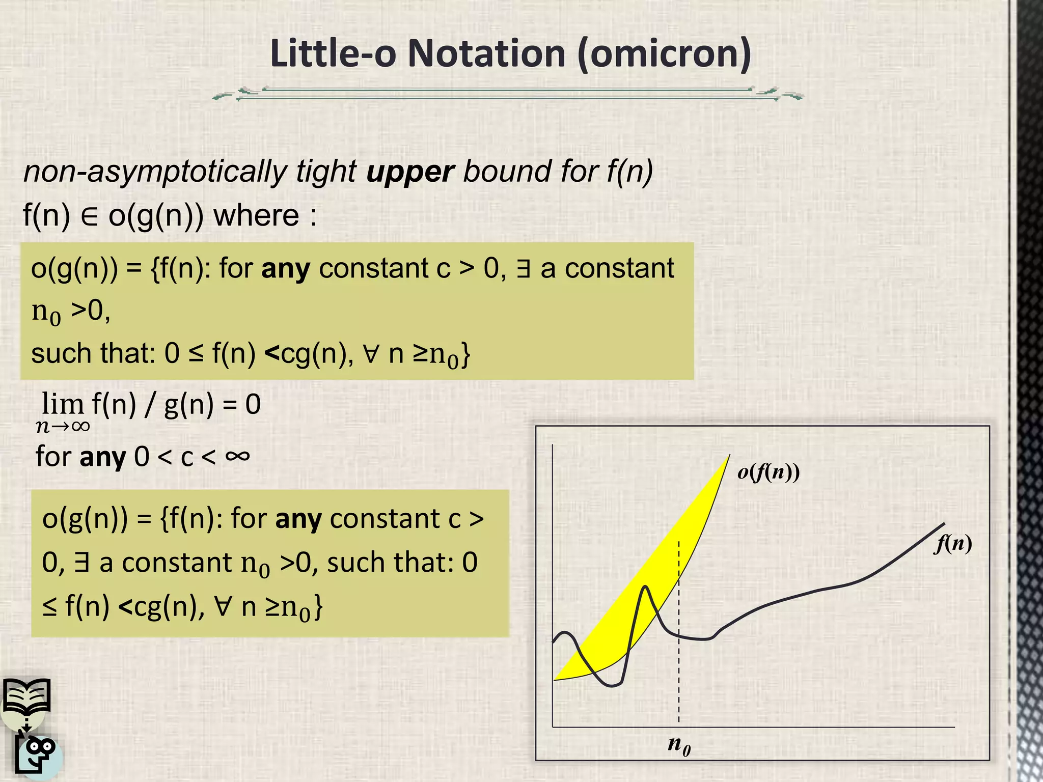
Little-o Notation (omicron)
non-asymptoticallytight upper bound for f(n)
f(n) ∈ o(g(n)) where :
lim
𝑛→∞
f(n) / g(n) = 0
for any 0 < c < ∞
o(g(n)) = {f(n): for any constant c >
0, ∃ a constant n0 >0, such that: 0
≤ f(n) <cg(n), ∀ n ≥n0}
o(g(n)) = {f(n): for any constant c > 0, ∃ a constant
n0 >0,
such that: 0 ≤ f(n) <cg(n), ∀ n ≥n0}
o(f(n))
f(n)
n0
16.
Little-ω Notation (omega)
non-asymptoticallytight lower bound for f(n)
f(n) ∈ ω(g(n)) where :
for any 0 < c ≤ ∞
lim
𝑛→∞
f(n) / g(n) = c
for some 0 < c ≤ ∞
Ω possibly asymptotically tight lower bound
ω non-asymptotically tight lower bound
ω(g(n)) = {f(n): for any constant c > 0, ∃ a constant n0 >0,
such that 0 ≤ cg(n) <f(n), ∀ n ≥n0}
Ω(g(n)) = {f(n): for some constant c > 0, ∃ a
constant n0 >0, such that 0 ≤ cg(n) ≤ f(n),
∀ n ≥n0}
lim
𝑛→∞
f(n) / g(n) = ∞
(f(n))
f(n)
n0
17.
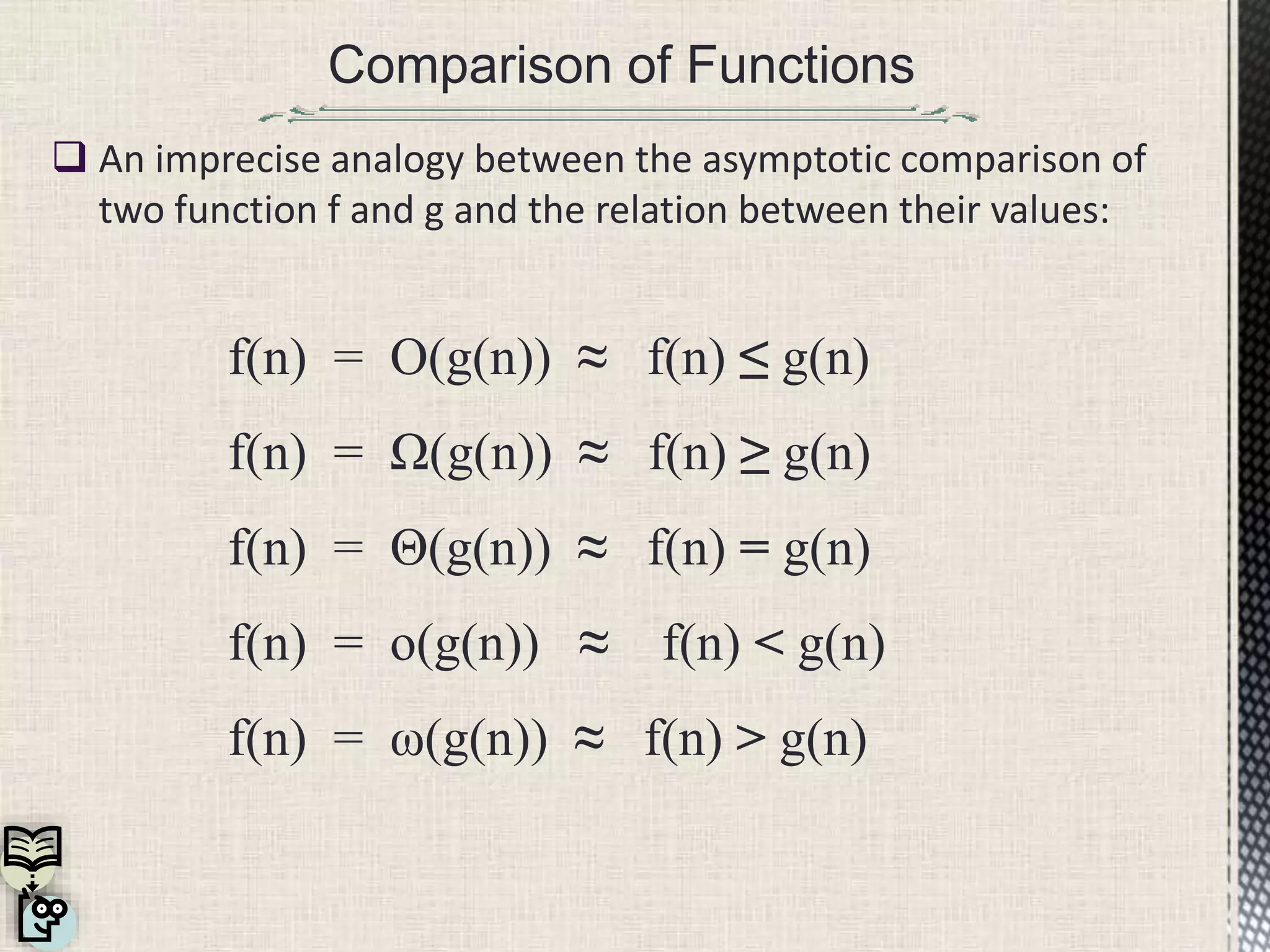
Comparison of Functions
An imprecise analogy between the asymptotic comparison of
two function f and g and the relation between their values:
f(n) = O(g(n)) ≈ f(n) ≤ g(n)
f(n) = Ω(g(n)) ≈ f(n) ≥ g(n)
f(n) = Θ(g(n)) ≈ f(n) = g(n)
f(n) = o(g(n)) ≈ f(n) < g(n)
f(n) = ω(g(n)) ≈ f(n) > g(n)
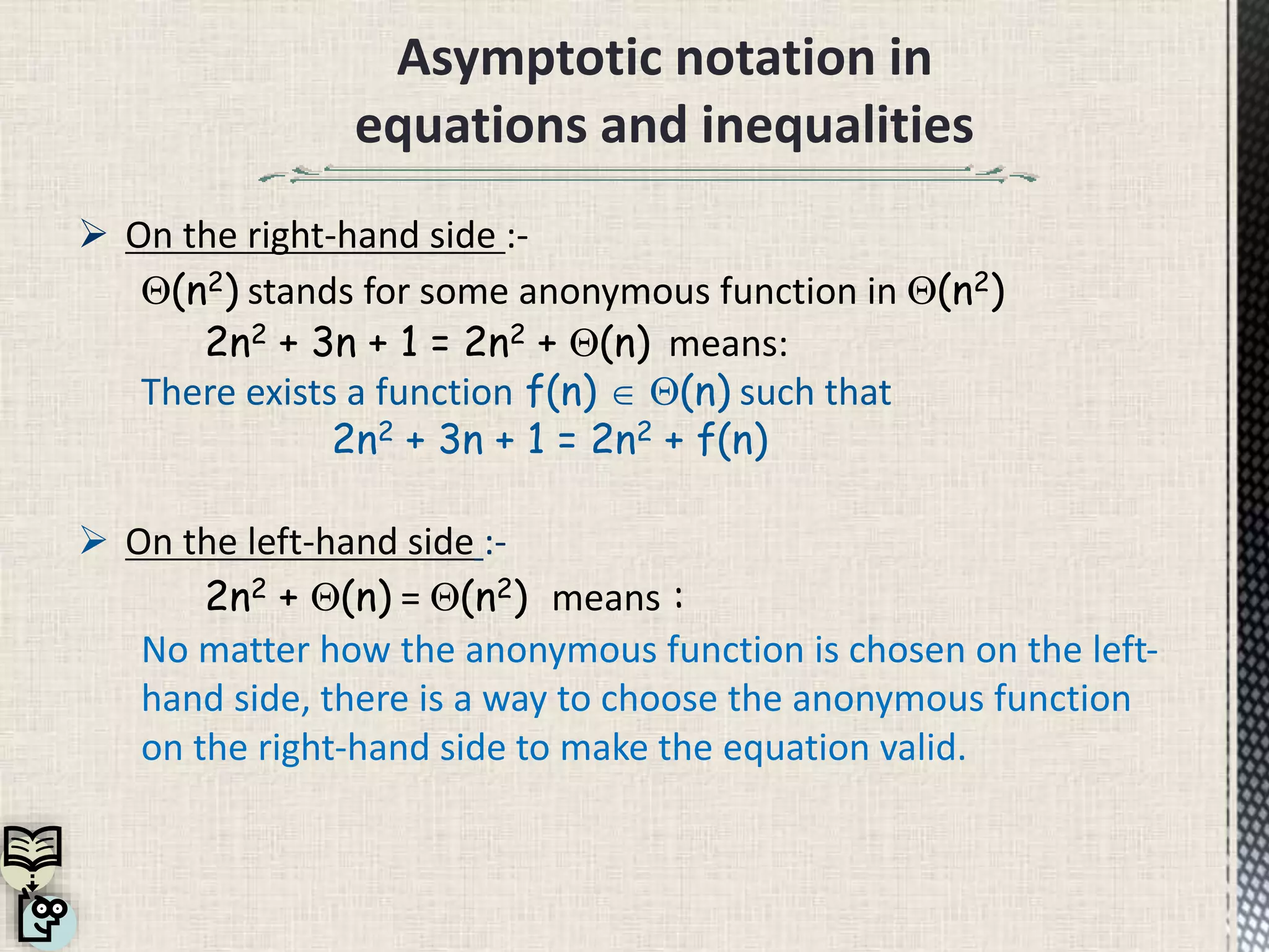
Asymptotic notation in
equationsand inequalities
On the right-hand side :-
(n2) stands for some anonymous function in (n2)
2n2 + 3n + 1 = 2n2 + (n) means:
There exists a function f(n) (n) such that
2n2 + 3n + 1 = 2n2 + f(n)
On the left-hand side :-
2n2 + (n) = (n2) means :
No matter how the anonymous function is chosen on the left-
hand side, there is a way to choose the anonymous function
on the right-hand side to make the equation valid.
21.
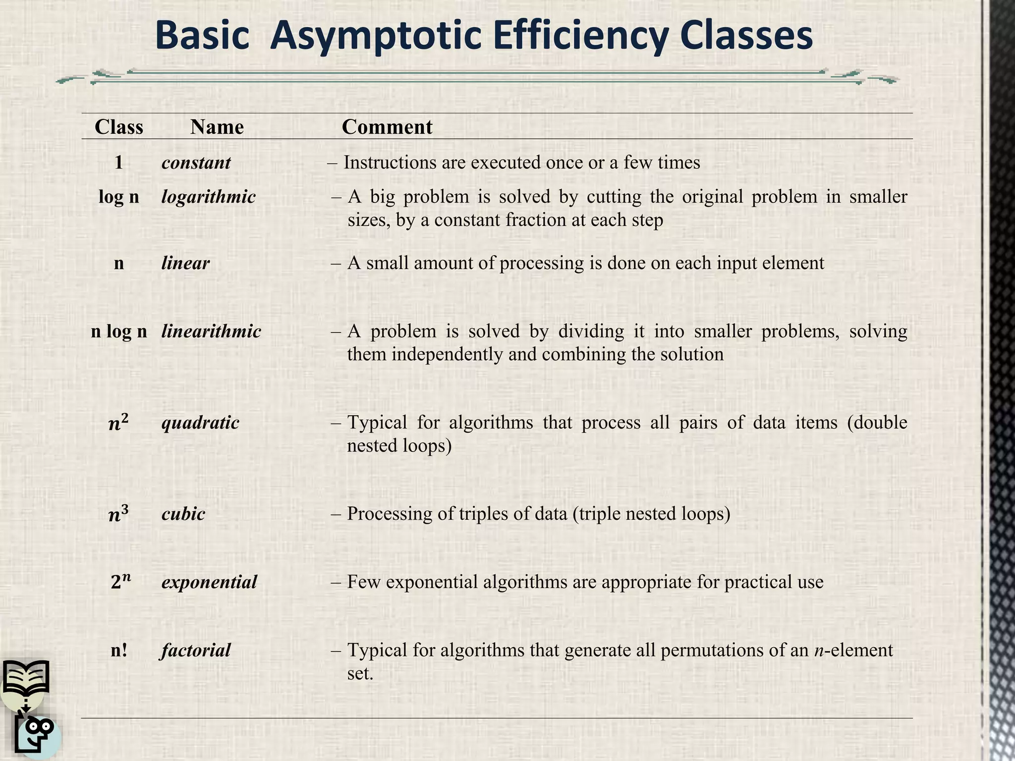
Class Name Comment
1constant – Instructions are executed once or a few times
log n logarithmic – A big problem is solved by cutting the original problem in smaller
sizes, by a constant fraction at each step
n linear – A small amount of processing is done on each input element
n log n linearithmic – A problem is solved by dividing it into smaller problems, solving
them independently and combining the solution
𝒏 𝟐 quadratic – Typical for algorithms that process all pairs of data items (double
nested loops)
𝒏 𝟑 cubic – Processing of triples of data (triple nested loops)
𝟐 𝒏 exponential – Few exponential algorithms are appropriate for practical use
n! factorial – Typical for algorithms that generate all permutations of an n-element
set.
22.
Acknowledgement
Firstly , Iwould like to thanks Mr. Abhishek
Mukhopadhyay for giving us such an interesting
topic to work with and Of course last but not the
least I express my esteemed gratitude to my group
members Meraj,Papiya,Nazaan,Protap who put up
with me during the whole period and provided me
valuable guidance in times of need and gave
wonderful cooperation and support to complete
the project.

![lim [f(n) / g(n)] = 0 f(n) o(g(n))
n
lim [f(n) / g(n)] < f(n) O(g(n))
n
0 < lim [f(n) / g(n)] < f(n) (g(n))
n
0 < lim [f(n) / g(n)] f(n) W(g(n))
n
Lim [f(n) / g(n)] = f(n) (g(n))
n
lim [f(n) / g(n)] undefined can’t say
n
Limits](https://image.slidesharecdn.com/pptproject-160622052244/75/Asymptotic-Notation-18-2048.jpg)


![lim [f(n) / g(n)] = 0 f(n) o(g(n))
n
lim [f(n) / g(n)] < f(n) O(g(n))
n
0 < lim [f(n) / g(n)] < f(n) (g(n))
n
0 < lim [f(n) / g(n)] f(n) W(g(n))
n
Lim [f(n) / g(n)] = f(n) (g(n))
n
lim [f(n) / g(n)] undefined can’t say
n
Limits](https://crownmelresort.com/image.slidesharecdn.com/pptproject-160622052244/75/Asymptotic-Notation-18-2048.jpg)


![ANPARA THERMAL POWER STATION[1] sangam.pdf](https://cdn.slidesharecdn.com/ss_thumbnails/anparathermalpowerstation1sangam-251121115219-9261cde4-thumbnail.jpg?width=640&height=640&fit=bounds)


