Downloaded 13 times

![18
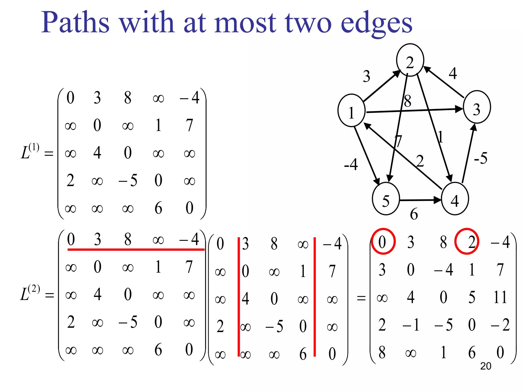
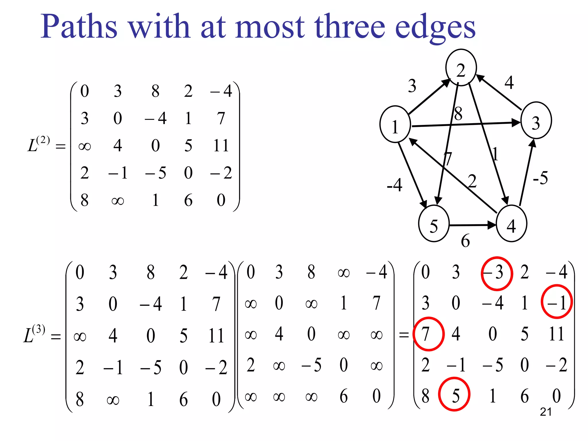
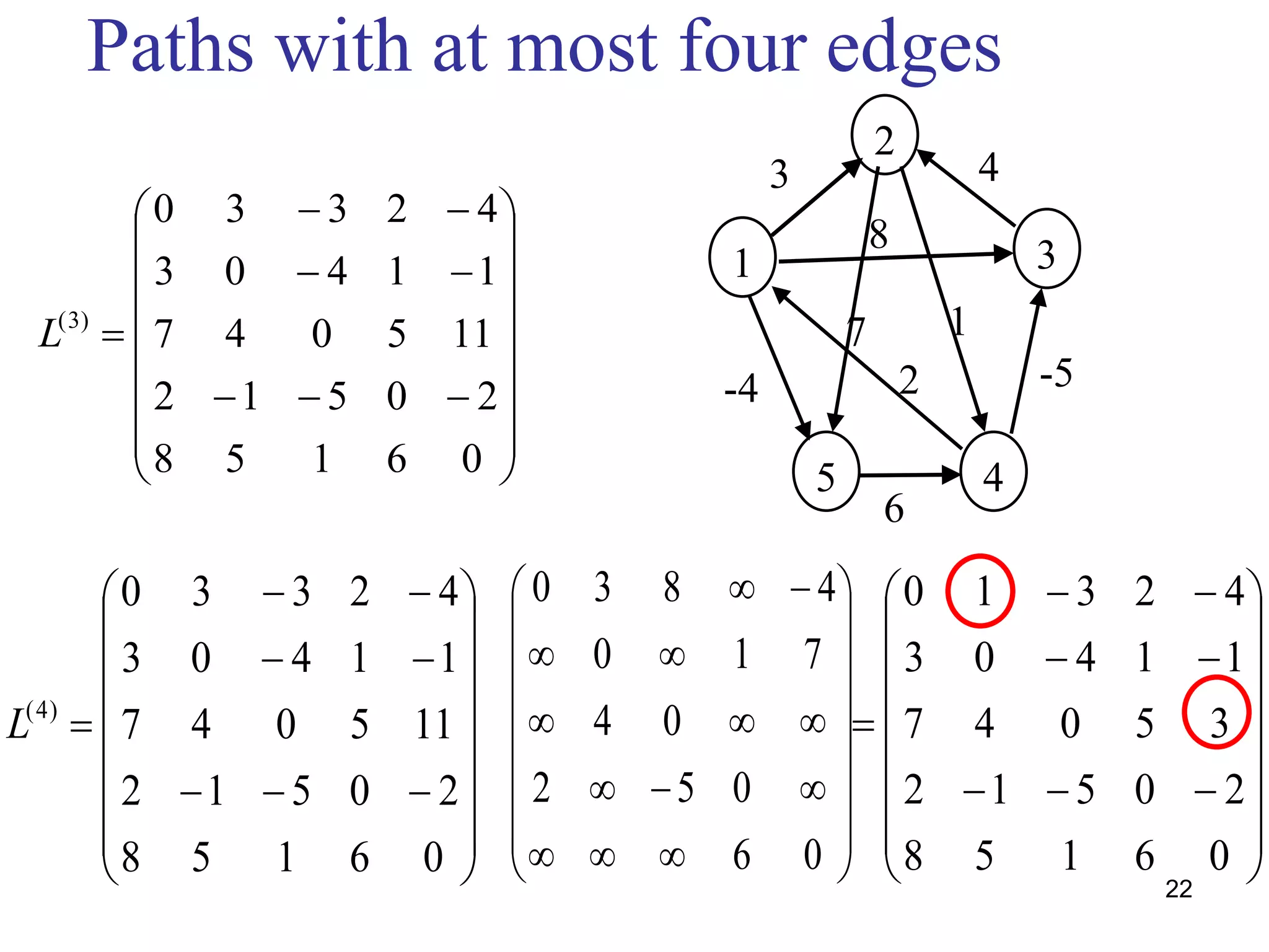
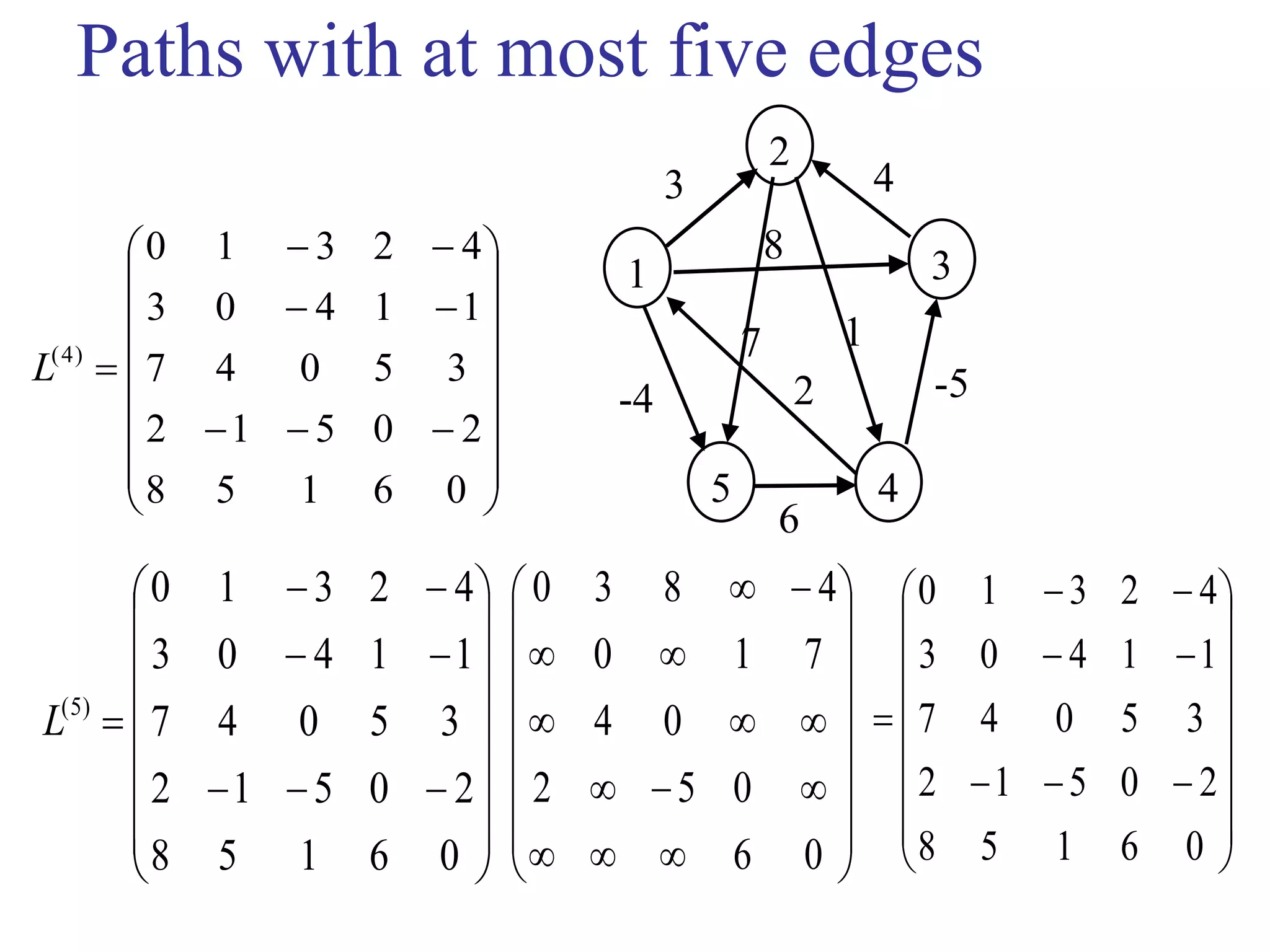
Algorithm for extending all-shortest
paths by one edge: from L(m-1) to L(m)
EXTEND-SHORTEST-PATHS(L=(lij),W)
n rows[L]
Let L’ =(l’ij) be an n×n matrix.
for i 1 to n do
for j 1 to n do
l’ij ∞
for k 1 to n do
l’ij min(l’ij, lik + wkj)
return L’
Complexity: Θ(|V|3)](https://image.slidesharecdn.com/chapter26aoa-190904110934/75/Chapter-26-aoa-18-2048.jpg)
![19
This is exactly as matrix
multiplication!
Matrix-Multiply(A,B)
n rows[A]
Let C =(cij) be an n×n matrix.
for i 1 to n do
for j 1 to n do
cij 0 (l’ij ∞)
for k 1 to n do
cij cij+ aik.bkj (l’ij min(l’ij, lij + wkj))
return L’
min
)(
)1(
cl
bw
al
m
m](https://image.slidesharecdn.com/chapter26aoa-190904110934/75/Chapter-26-aoa-19-2048.jpg)
![24
All-shortest Paths Algorithm
SLOW-ALL-PAIRS-SHORTEST-PATHS(W)
1. n rows[W]
2. L(1) W
3. for m 2 to n–1 do
4. L(m) Extend-Shortest-Paths(L(m–1),W)
5. return L(m)
Complexity: Θ(|V|4)](https://image.slidesharecdn.com/chapter26aoa-190904110934/75/Chapter-26-aoa-24-2048.jpg)
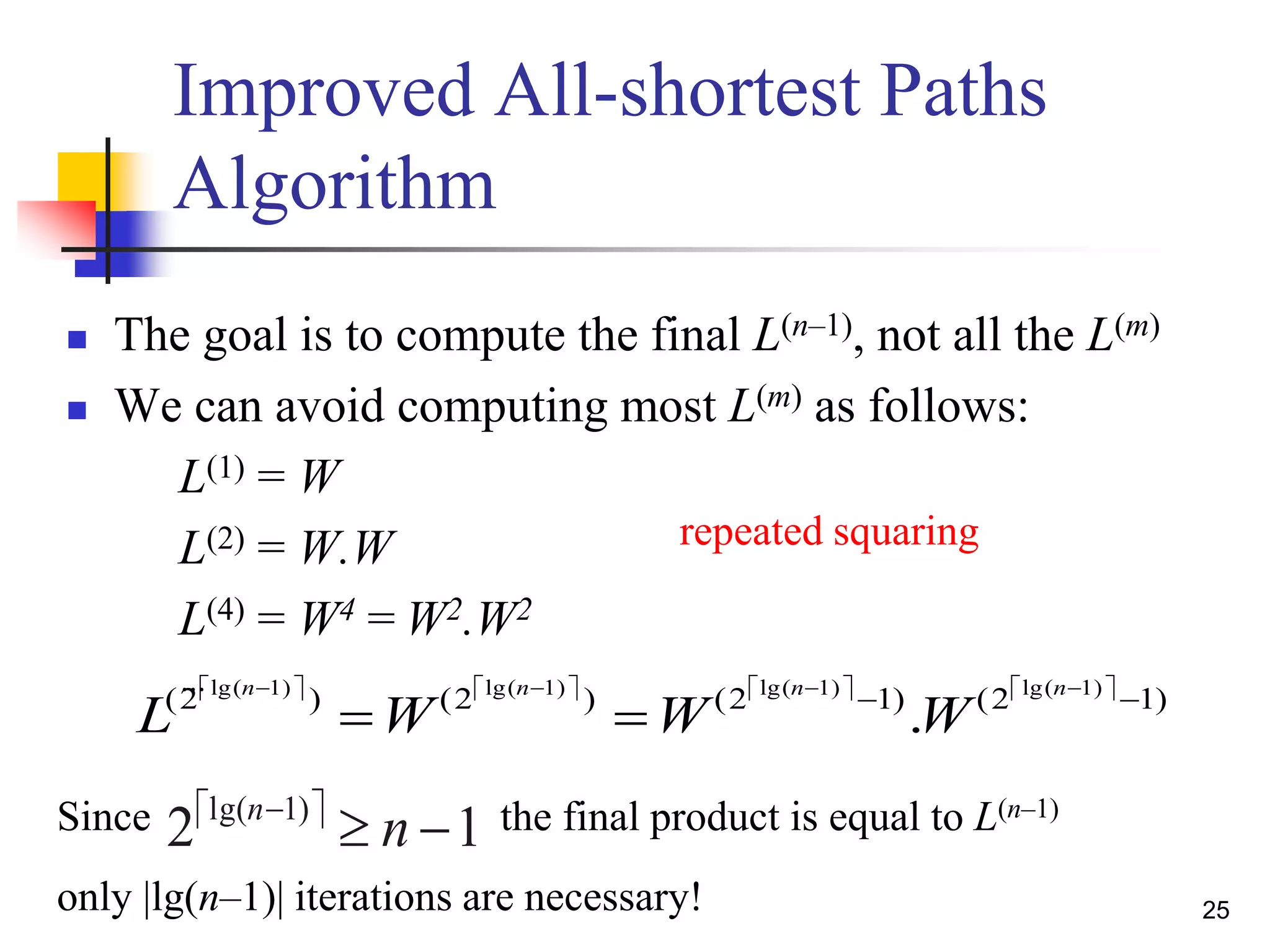
![26
Faster-All-Shortest Paths
Algorithm
FASTER-ALL-PAIRS-SHORTEST-PATHS(W)
1. n rows[W]
2. L(1) W
3. m 1
4. while m < n–1 do
5. L(2m) Extend-Shortest-Paths(L(m),L(m))
6. m 2m
7. return L(m)
Complexity: Θ(|V|3 lg (|V|))](https://image.slidesharecdn.com/chapter26aoa-190904110934/75/Chapter-26-aoa-26-2048.jpg)
![Check Whether it works?
Dr. Hanif Durad 27
06
052
04
710
4830
)1(
L
06158
20512
35047
11403
42310
)4(
L
0618
20512
11504
71403
42830
)2(
L
35
(4
4
7
) [ 4 0511] 11 min(11, 4,4 7,0 11,5 2,11 0)
2
0
l
YES](https://image.slidesharecdn.com/chapter26aoa-190904110934/75/Chapter-26-aoa-27-2048.jpg)
![48
Transitive Closure Algorithm (3/3)
Complexity: Θ(|V|3)
TRANSITIVE-CLOSURE(G)
1 | [ ]|n V G
2 for i 1 to n
3 do for j 1 to n
4 do if i j or ( , ) ( )i j E G
5 then tij
( )0
1
6 else tij
( )0
0
7 for k 1 to n
8 do for i 1 to n
9 do for j 1 to n
10 do t t t tij
k
ij
k
ik
k
kj
k( ) ( ) ( ) ( )
( ) 1 1 1
11 return T n( )](https://image.slidesharecdn.com/chapter26aoa-190904110934/75/Chapter-26-aoa-48-2048.jpg)


![18
Algorithm for extending all-shortest
paths by one edge: from L(m-1) to L(m)
EXTEND-SHORTEST-PATHS(L=(lij),W)
n rows[L]
Let L’ =(l’ij) be an n×n matrix.
for i 1 to n do
for j 1 to n do
l’ij ∞
for k 1 to n do
l’ij min(l’ij, lik + wkj)
return L’
Complexity: Θ(|V|3)](https://crownmelresort.com/image.slidesharecdn.com/chapter26aoa-190904110934/75/Chapter-26-aoa-18-2048.jpg)
![19
This is exactly as matrix
multiplication!
Matrix-Multiply(A,B)
n rows[A]
Let C =(cij) be an n×n matrix.
for i 1 to n do
for j 1 to n do
cij 0 (l’ij ∞)
for k 1 to n do
cij cij+ aik.bkj (l’ij min(l’ij, lij + wkj))
return L’
min
)(
)1(
cl
bw
al
m
m](https://crownmelresort.com/image.slidesharecdn.com/chapter26aoa-190904110934/75/Chapter-26-aoa-19-2048.jpg)


![24
All-shortest Paths Algorithm
SLOW-ALL-PAIRS-SHORTEST-PATHS(W)
1. n rows[W]
2. L(1) W
3. for m 2 to n–1 do
4. L(m) Extend-Shortest-Paths(L(m–1),W)
5. return L(m)
Complexity: Θ(|V|4)](https://crownmelresort.com/image.slidesharecdn.com/chapter26aoa-190904110934/75/Chapter-26-aoa-24-2048.jpg)

![26
Faster-All-Shortest Paths
Algorithm
FASTER-ALL-PAIRS-SHORTEST-PATHS(W)
1. n rows[W]
2. L(1) W
3. m 1
4. while m < n–1 do
5. L(2m) Extend-Shortest-Paths(L(m),L(m))
6. m 2m
7. return L(m)
Complexity: Θ(|V|3 lg (|V|))](https://crownmelresort.com/image.slidesharecdn.com/chapter26aoa-190904110934/75/Chapter-26-aoa-26-2048.jpg)
![Check Whether it works?
Dr. Hanif Durad 27
06
052
04
710
4830
)1(
L
06158
20512
35047
11403
42310
)4(
L
0618
20512
11504
71403
42830
)2(
L
35
(4
4
7
) [ 4 0511] 11 min(11, 4,4 7,0 11,5 2,11 0)
2
0
l
YES](https://crownmelresort.com/image.slidesharecdn.com/chapter26aoa-190904110934/75/Chapter-26-aoa-27-2048.jpg)


![48
Transitive Closure Algorithm (3/3)
Complexity: Θ(|V|3)
TRANSITIVE-CLOSURE(G)
1 | [ ]|n V G
2 for i 1 to n
3 do for j 1 to n
4 do if i j or ( , ) ( )i j E G
5 then tij
( )0
1
6 else tij
( )0
0
7 for k 1 to n
8 do for i 1 to n
9 do for j 1 to n
10 do t t t tij
k
ij
k
ik
k
kj
k( ) ( ) ( ) ( )
( ) 1 1 1
11 return T n( )](https://crownmelresort.com/image.slidesharecdn.com/chapter26aoa-190904110934/75/Chapter-26-aoa-48-2048.jpg)


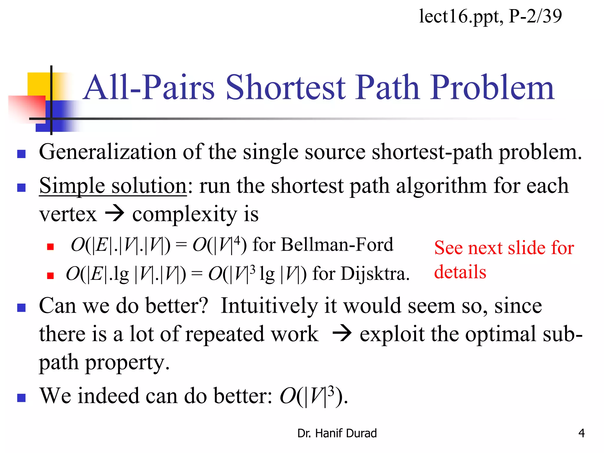
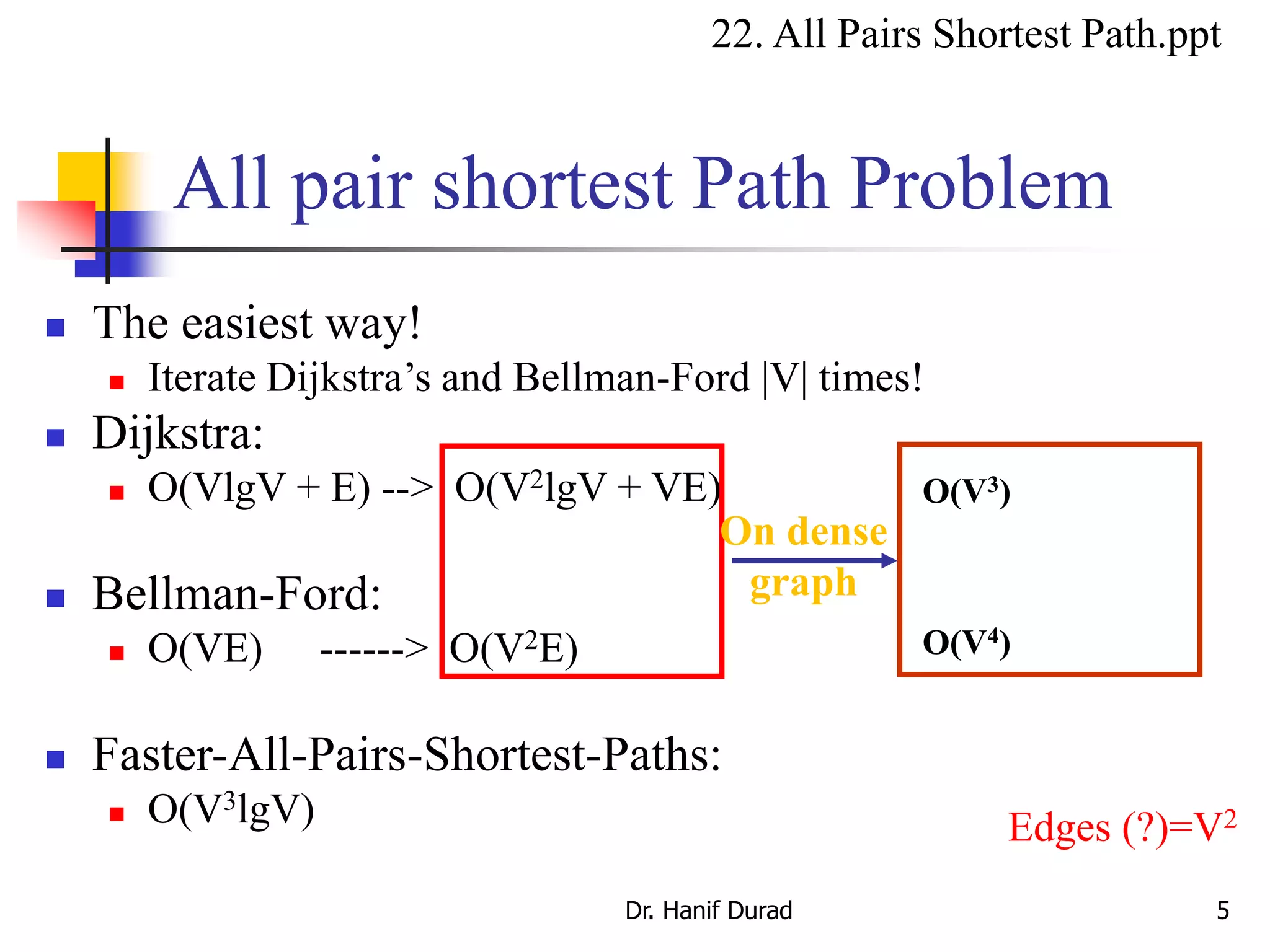
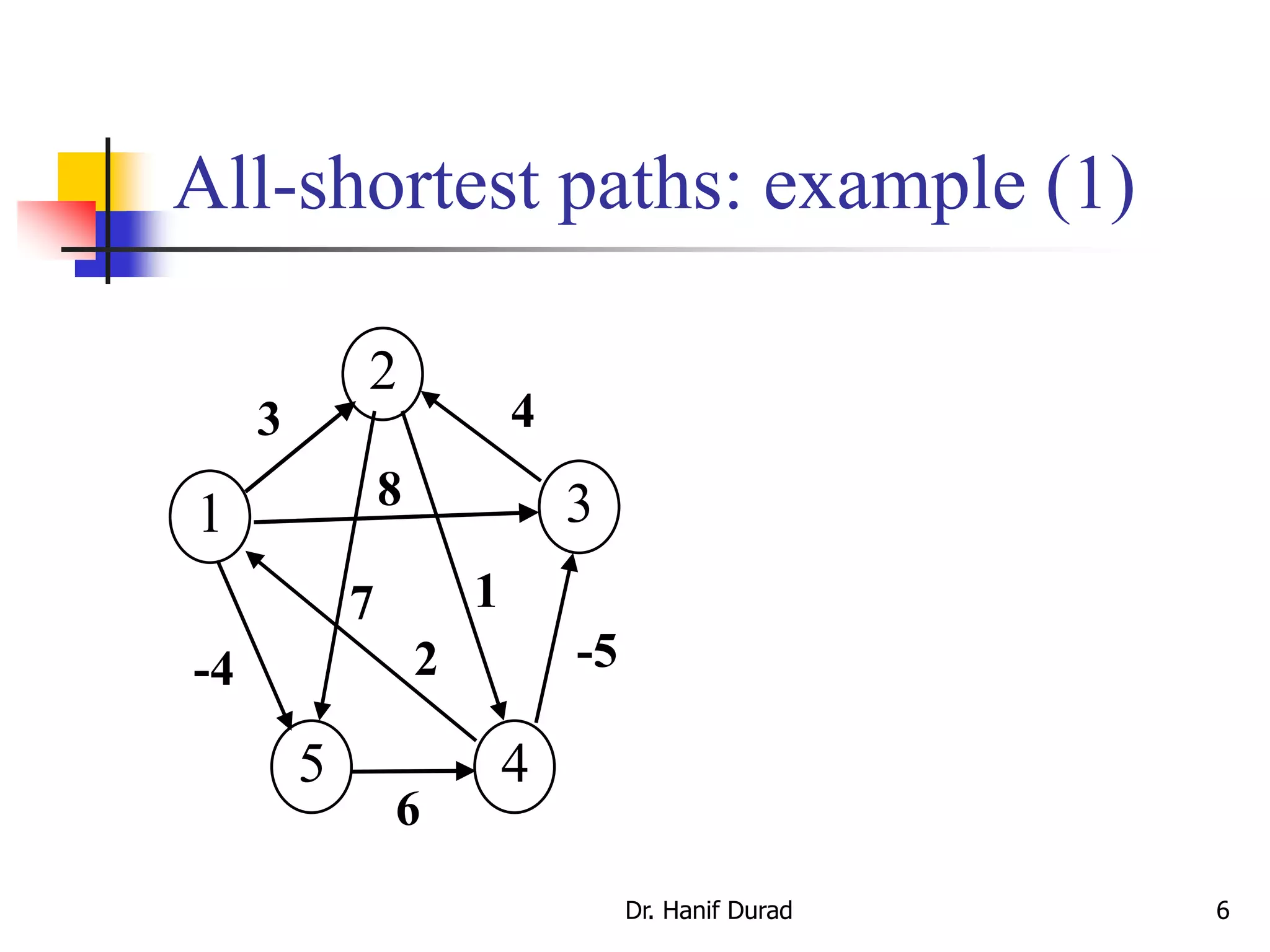
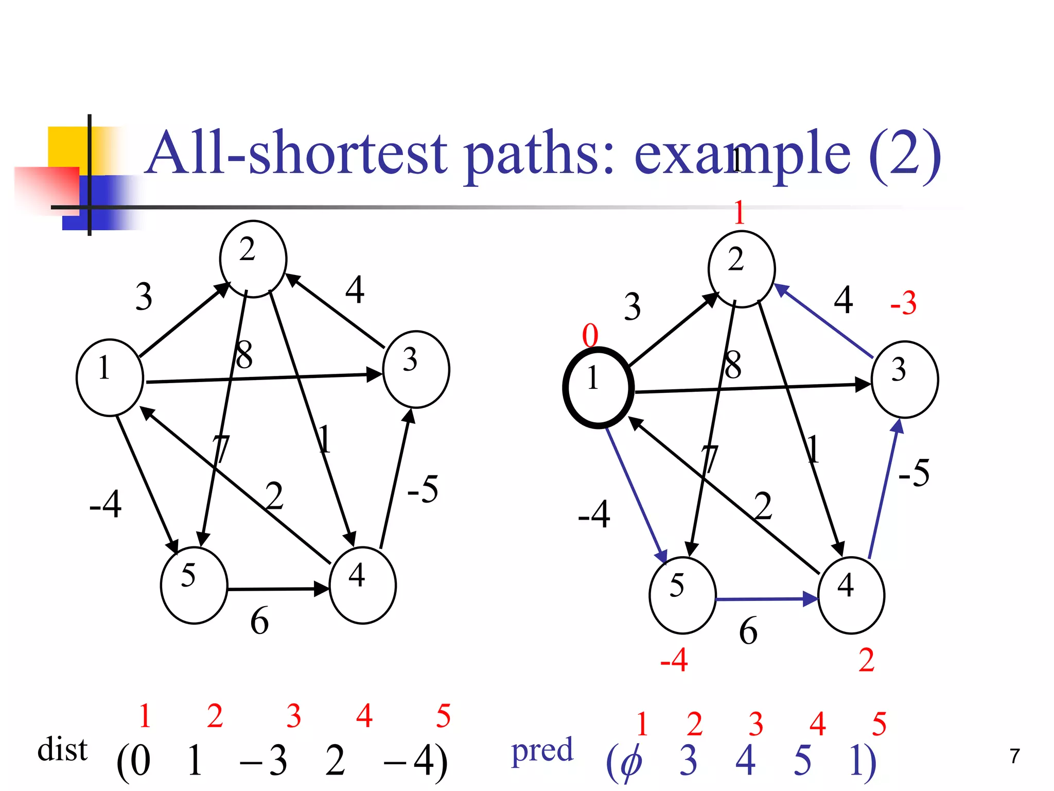
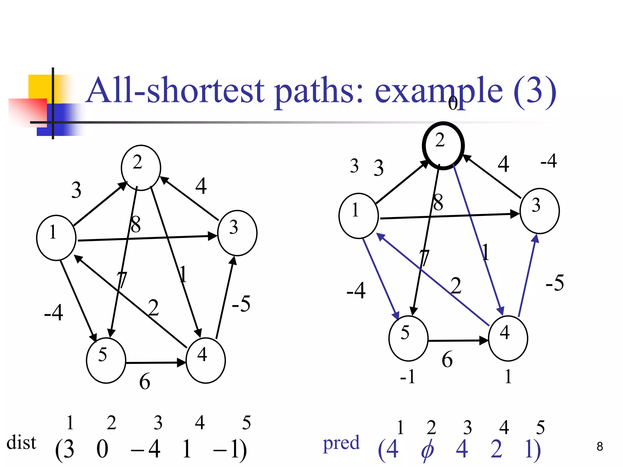
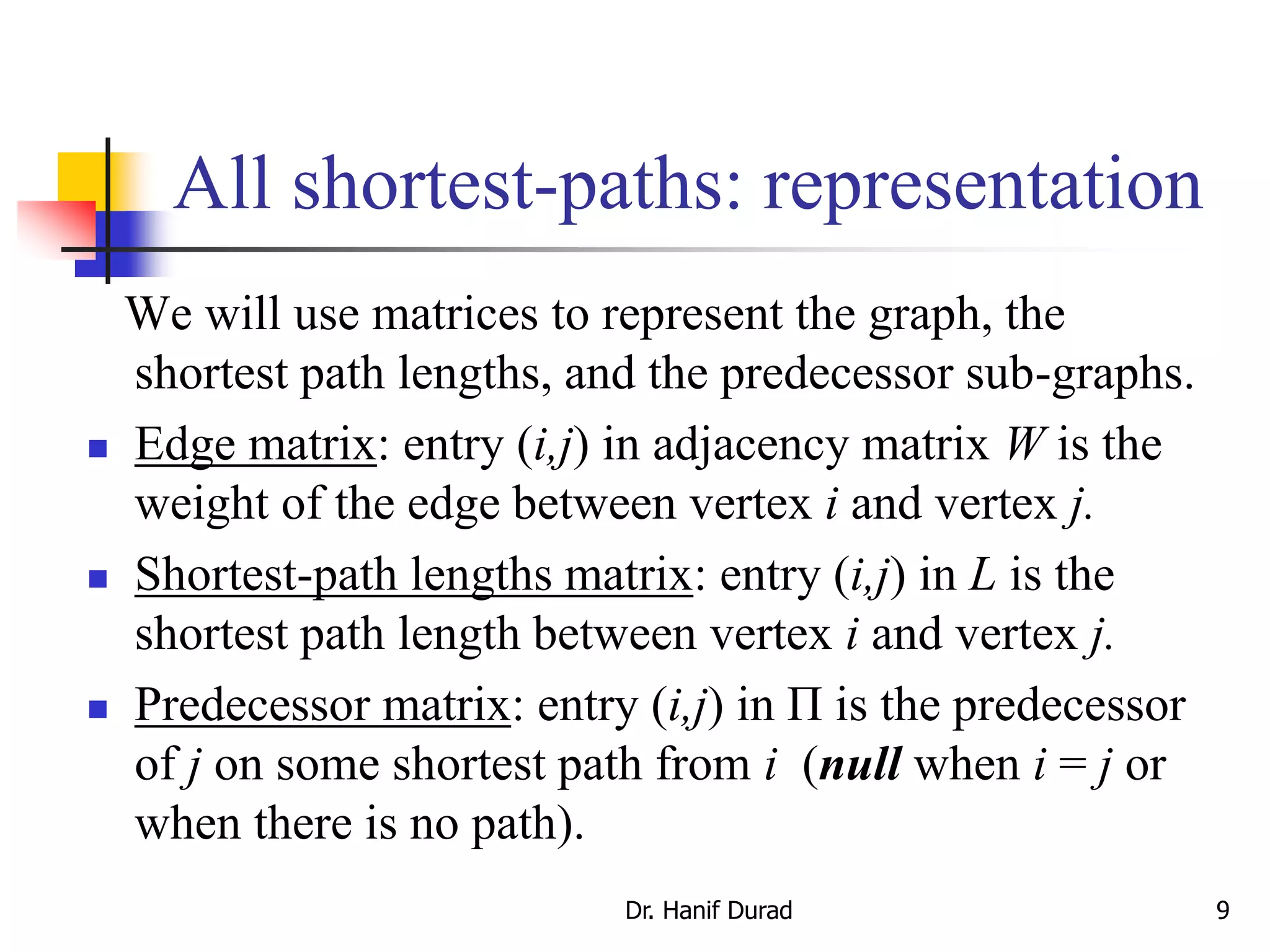
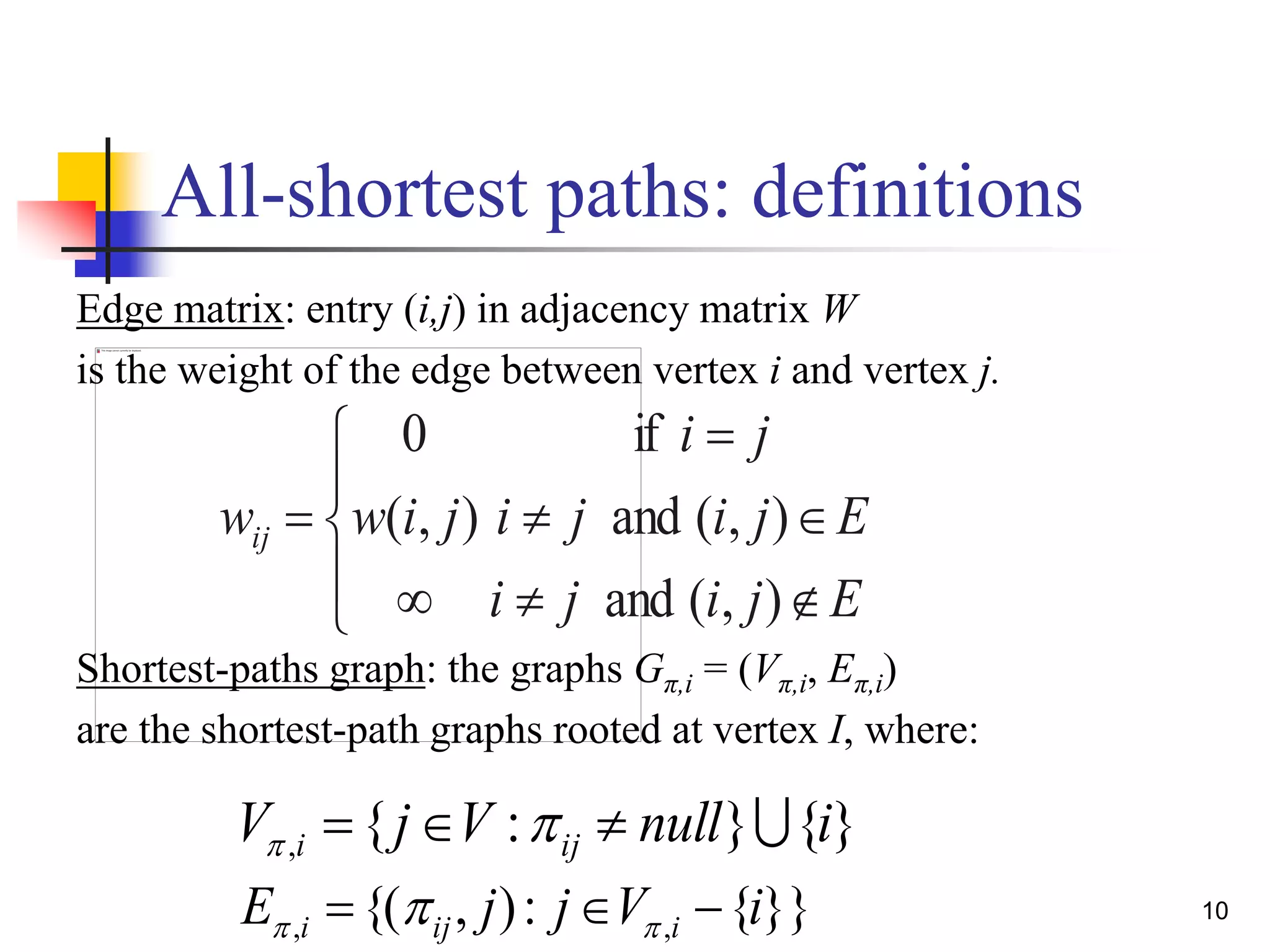
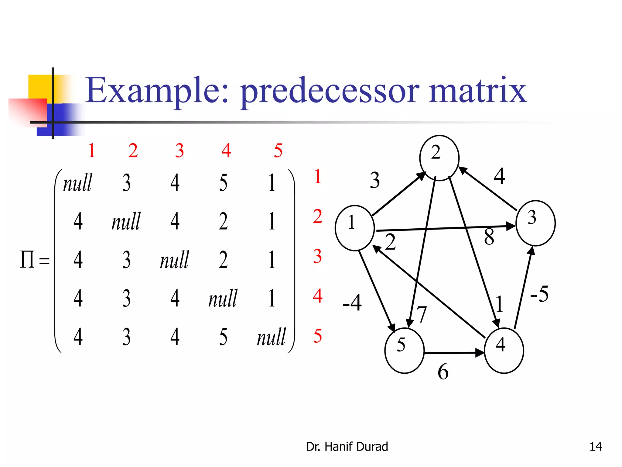
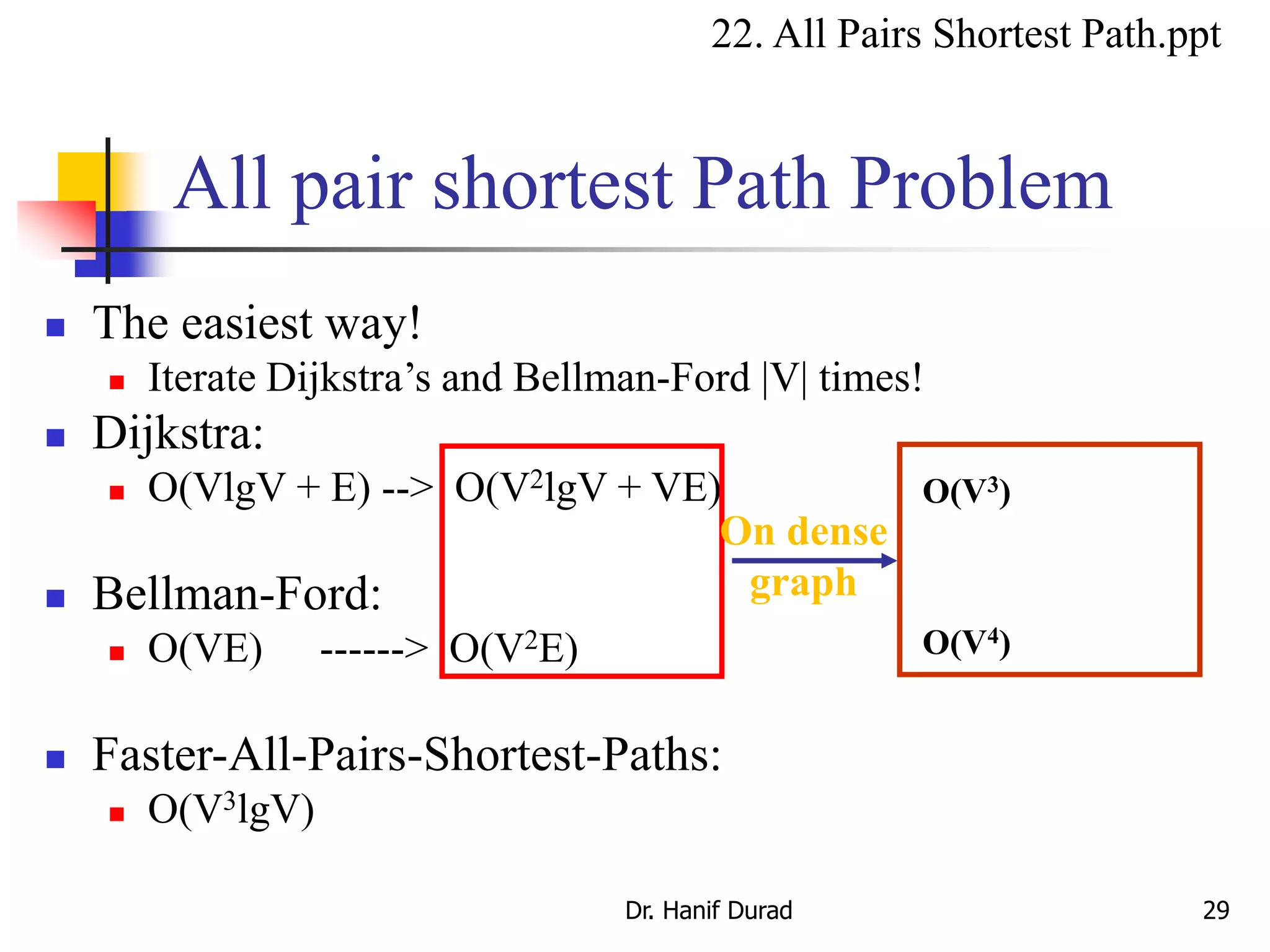
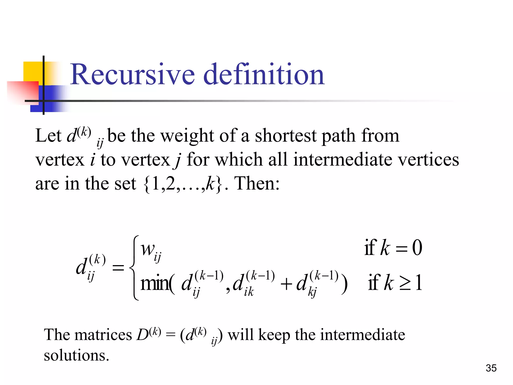
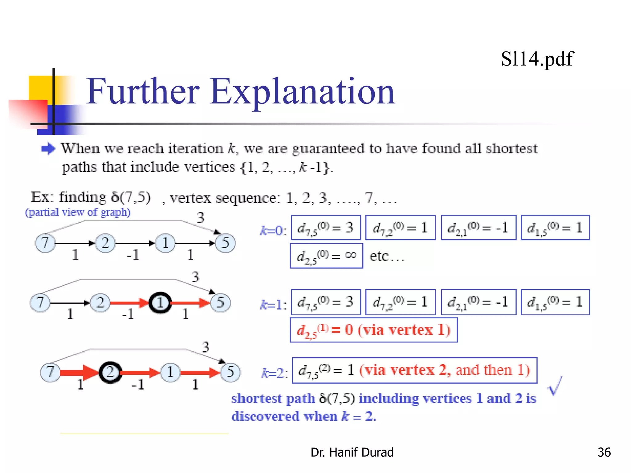
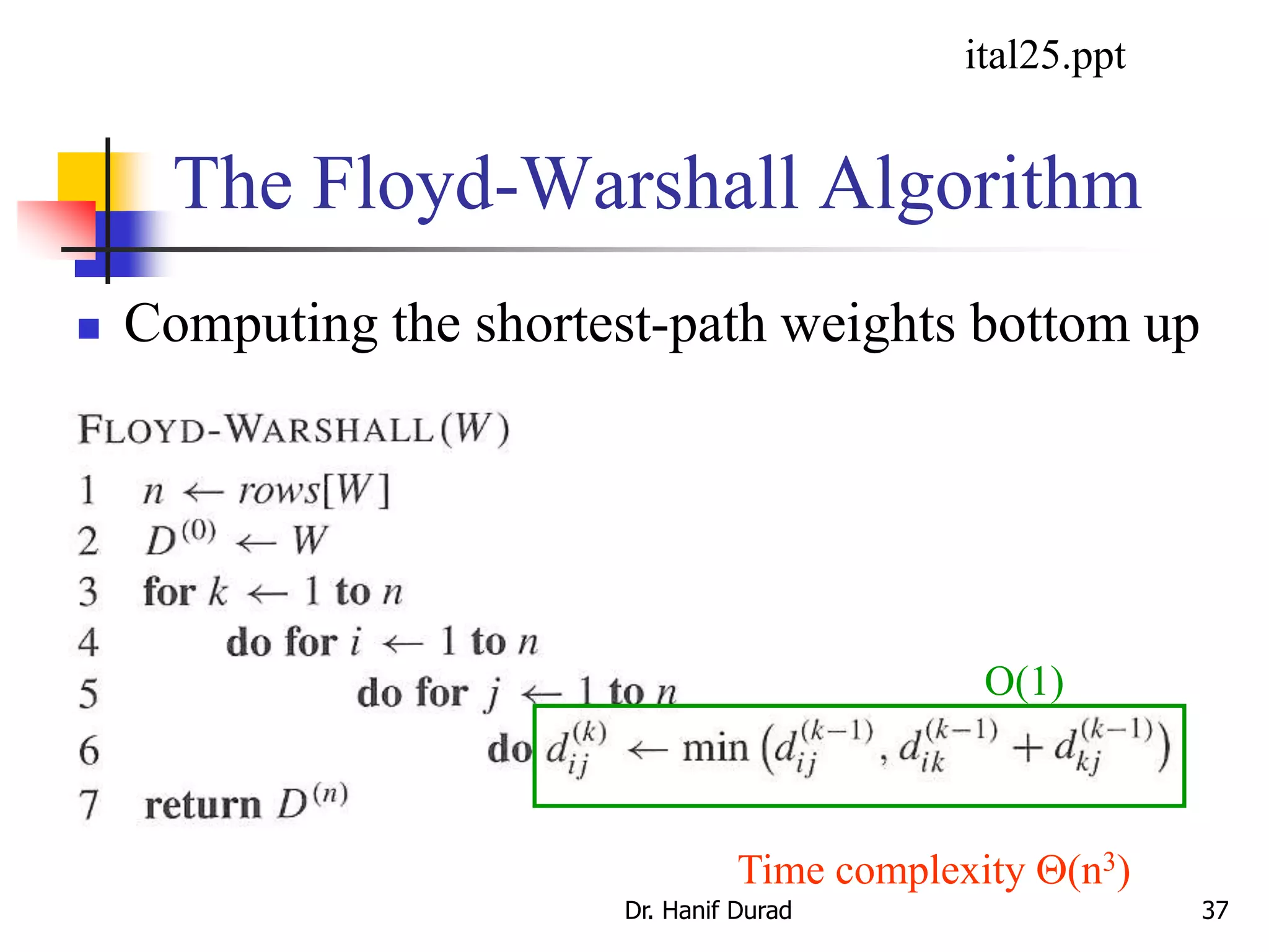
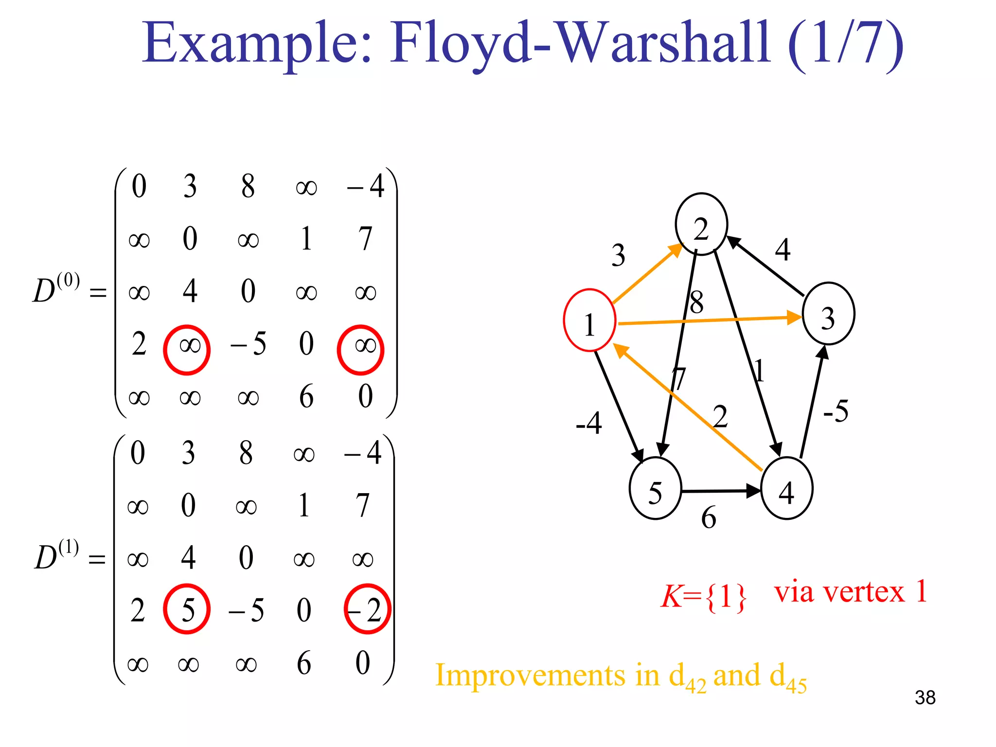
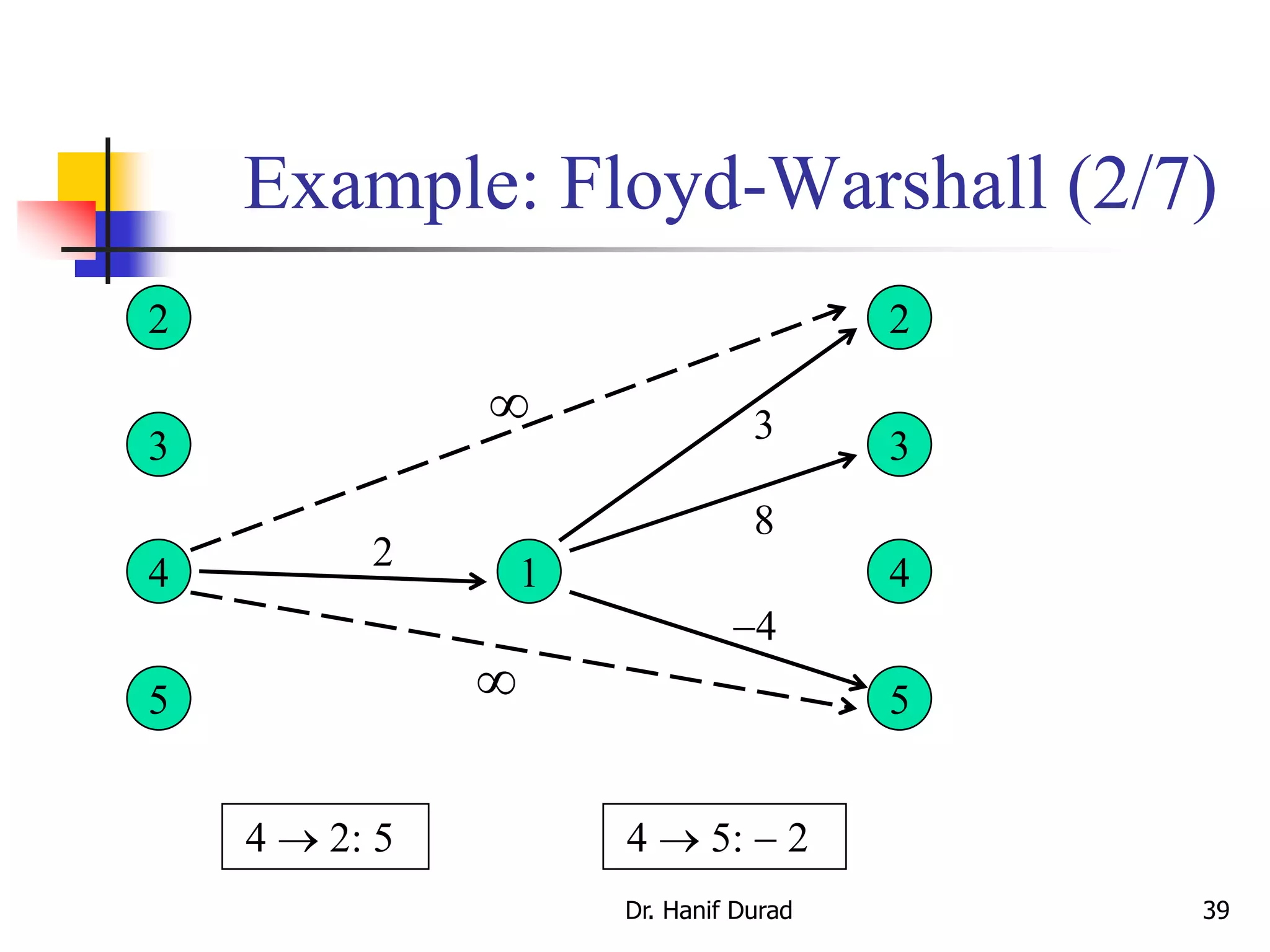
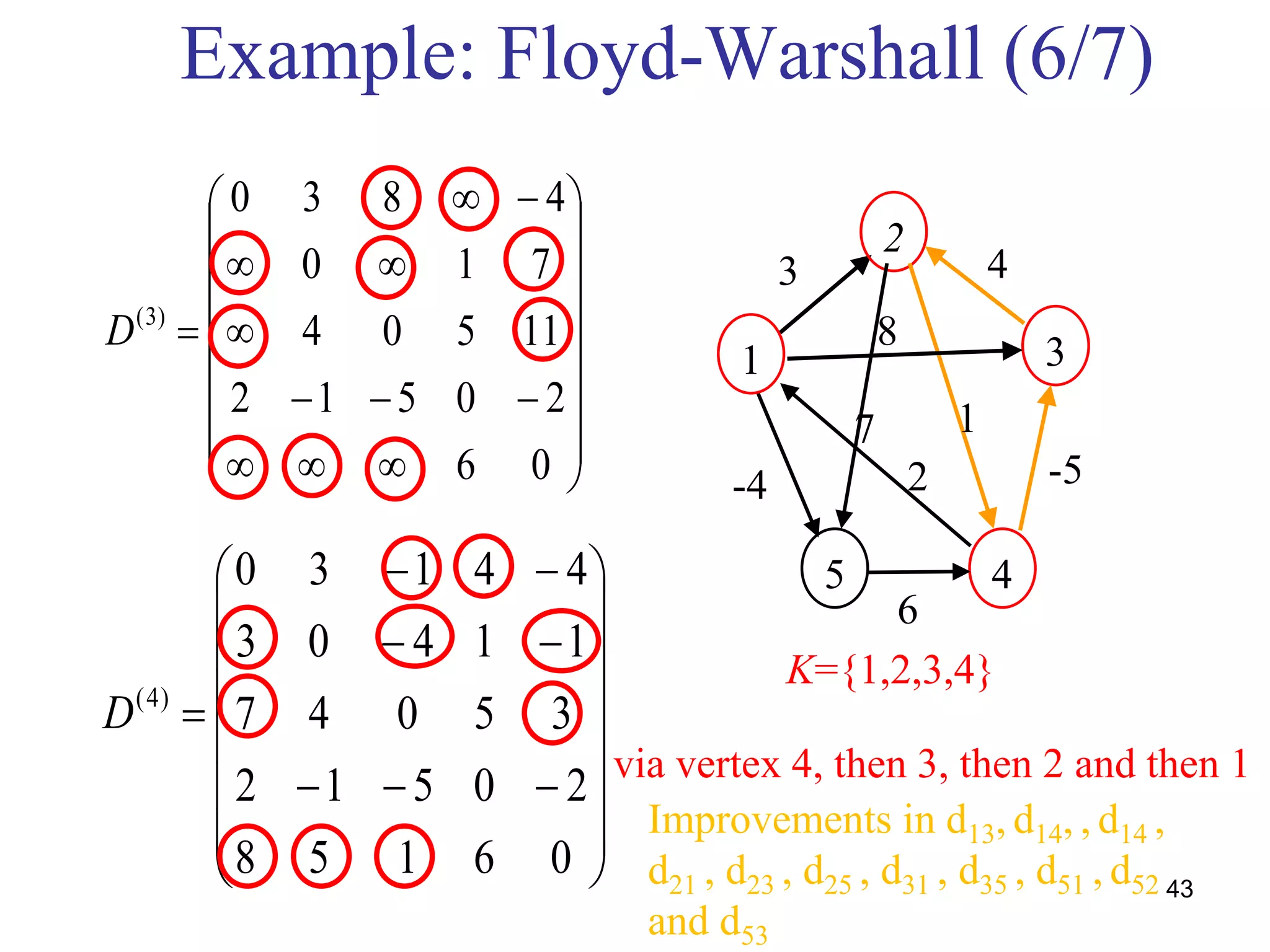
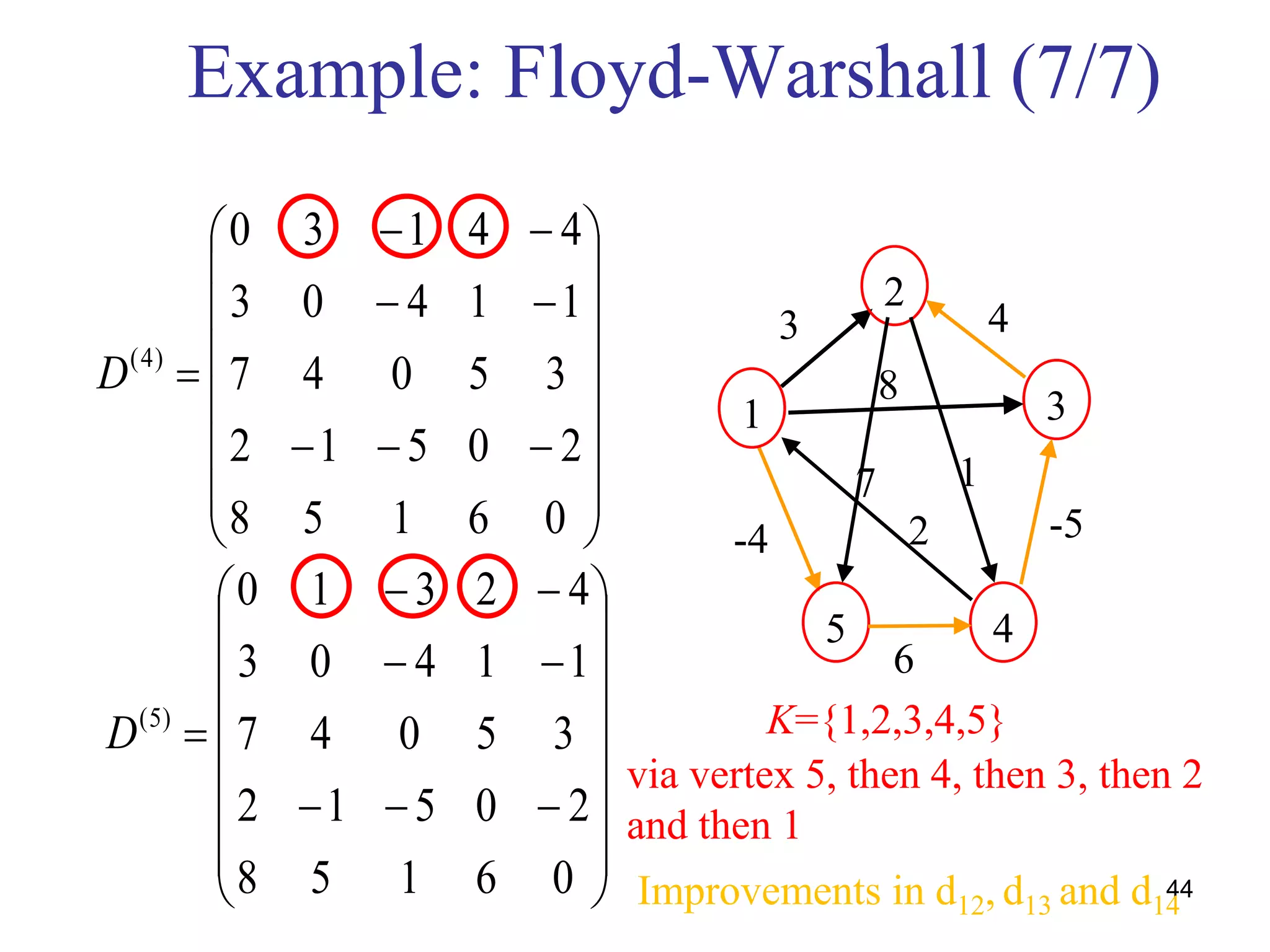
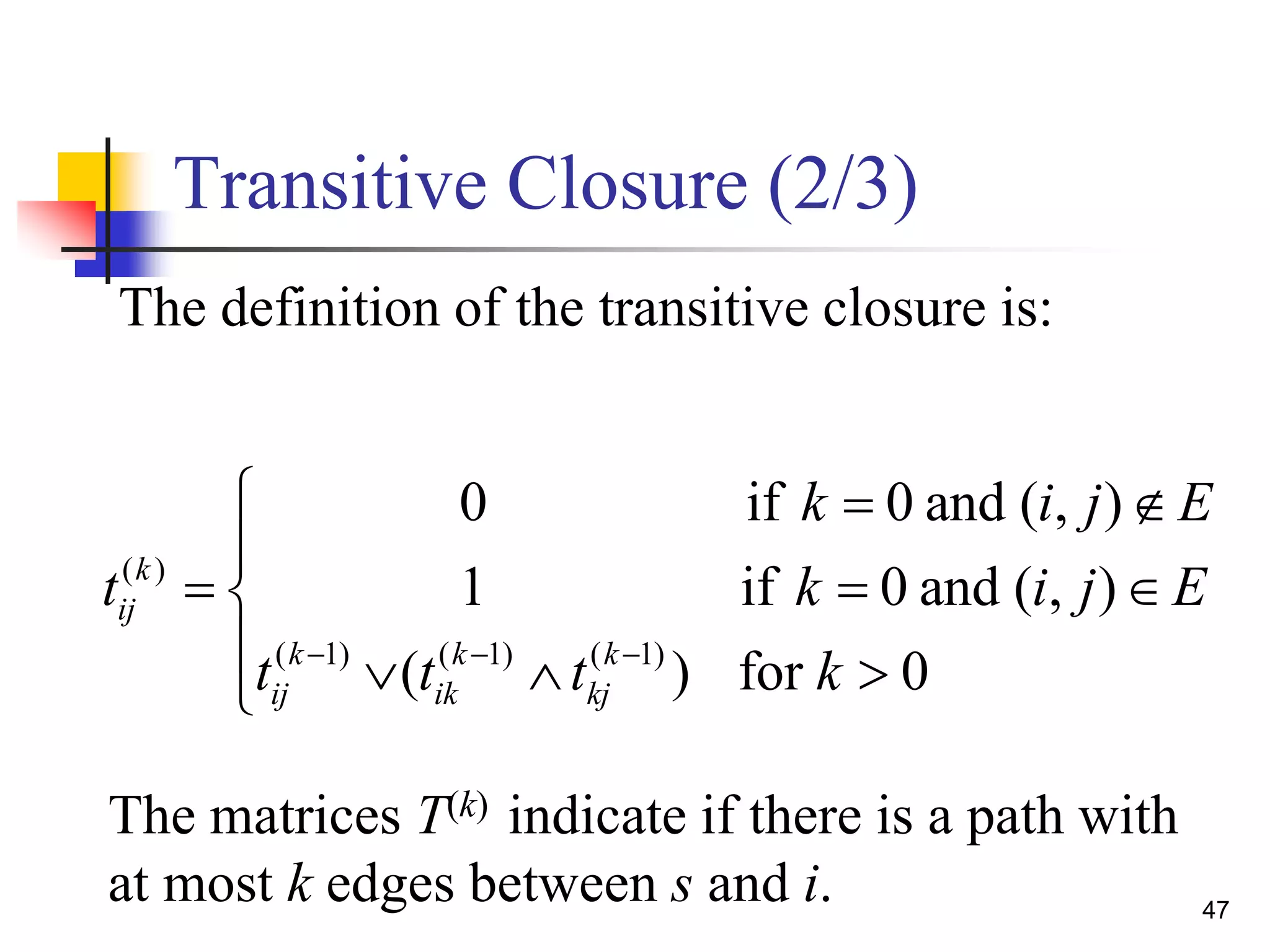
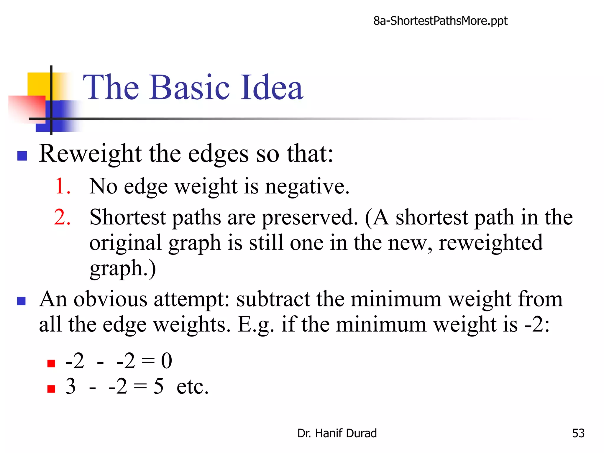
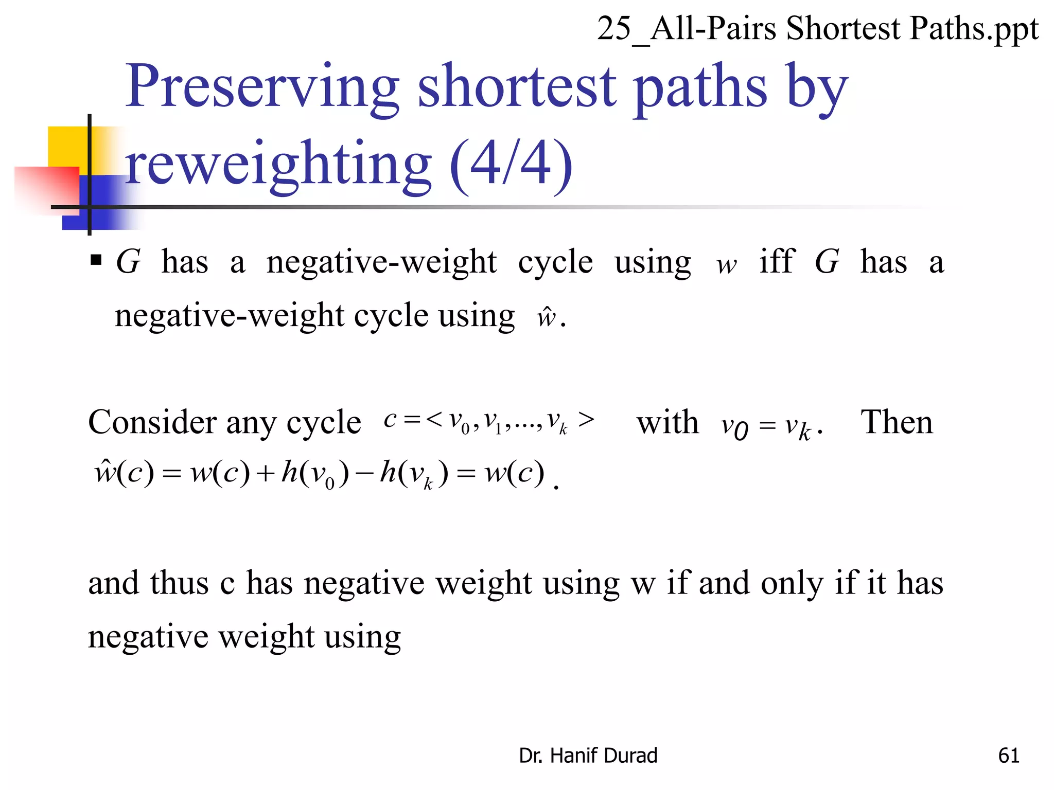
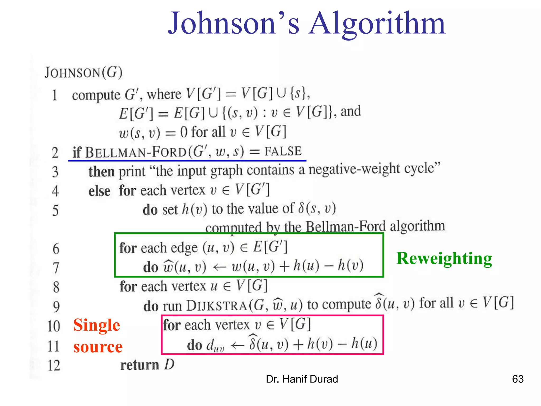
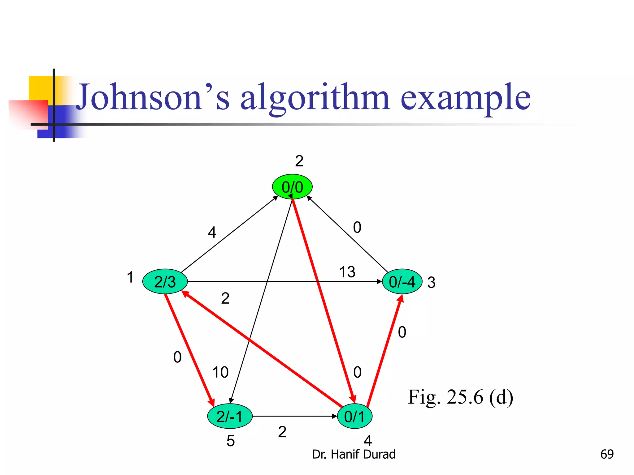
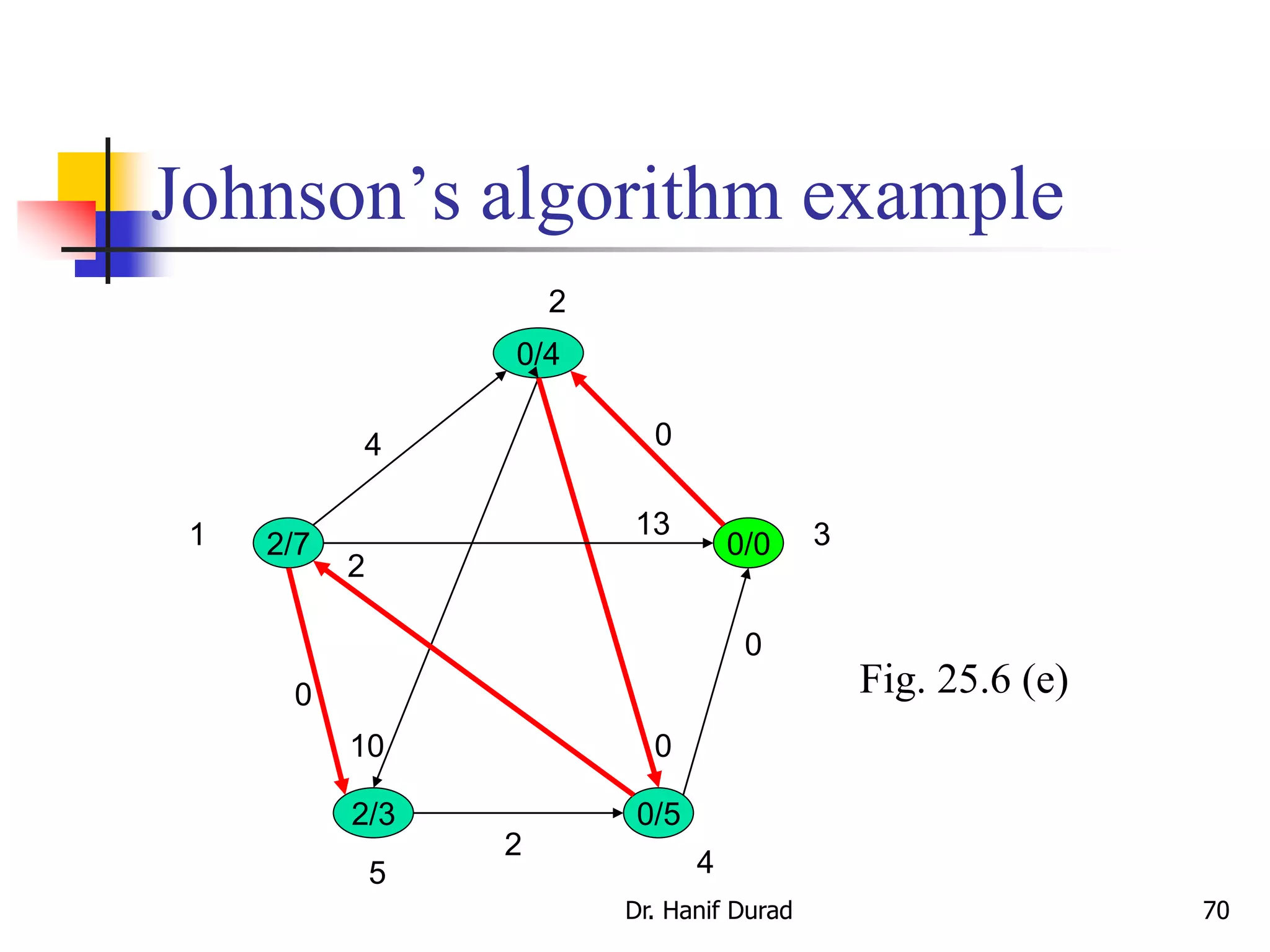
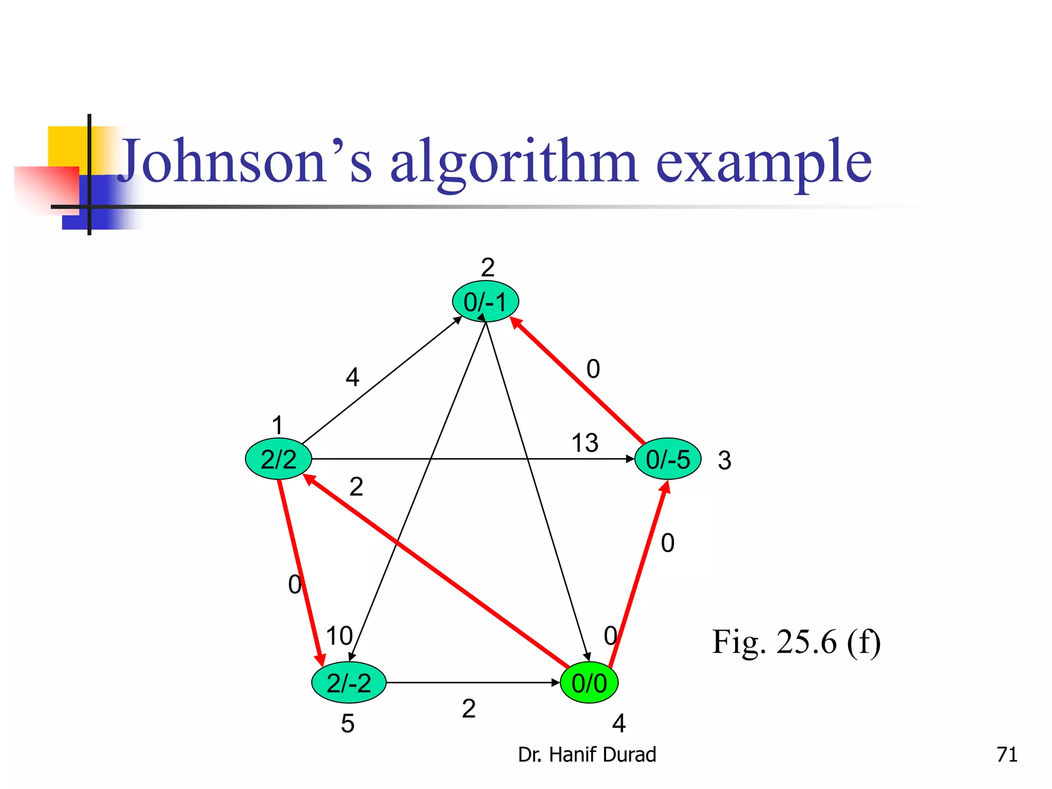
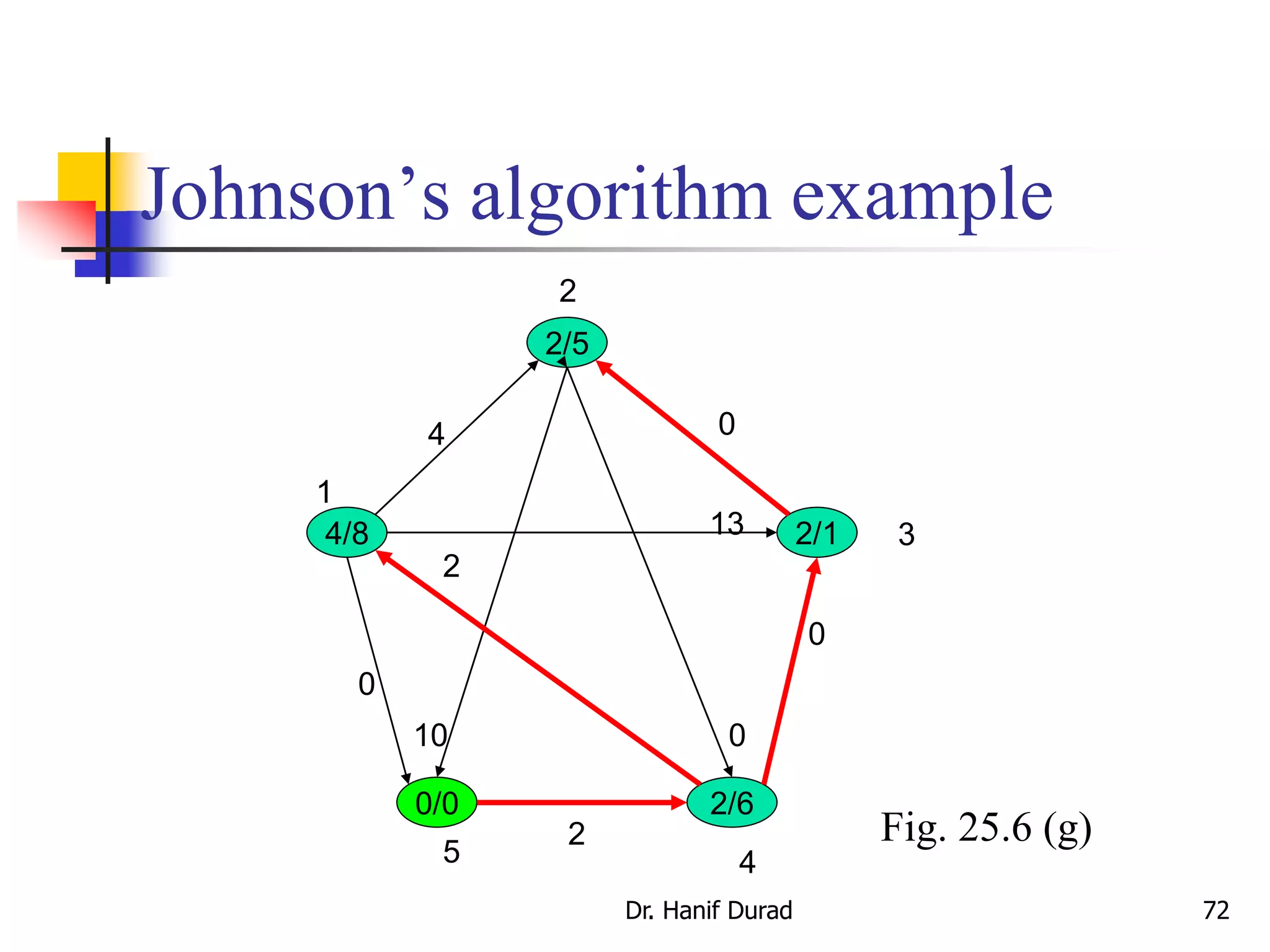
This document outlines the all-pairs shortest path problem and the Floyd-Warshall algorithm. It begins with an introduction to the problem and notes that naively running single-source shortest path algorithms would have a complexity of O(V4) or O(V3logV). It then provides an outline of the lecture which will cover all-pairs shortest paths, extending shortest paths, the Floyd-Warshall algorithm, analyzing shortest paths, and Johnson's algorithm for sparse graphs. The document provides examples and definitions to explain the representation of graphs, shortest path lengths, and predecessor matrices used in the algorithm. It also describes the recursive structure of shortest paths and how the Floyd-Warshall algorithm works by iteratively extending paths by one


![SHS_Core_CAE_Q3_LE1 FOR THIRD [FINAL].pdf](https://cdn.slidesharecdn.com/ss_thumbnails/shscorecaeq3le1final-251116055110-e3081055-thumbnail.jpg?width=640&height=640&fit=bounds)


