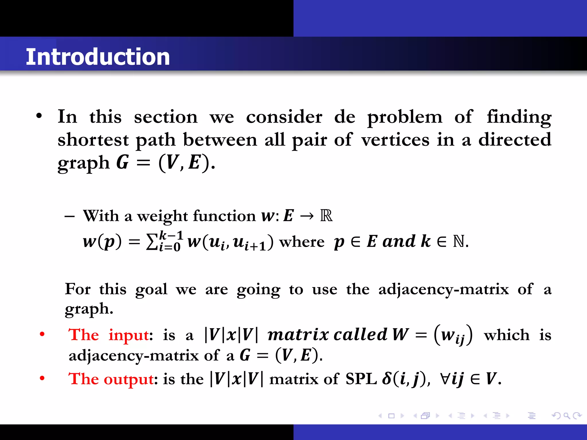
The document discusses algorithms for finding shortest paths between all pairs of vertices in a directed graph, including:
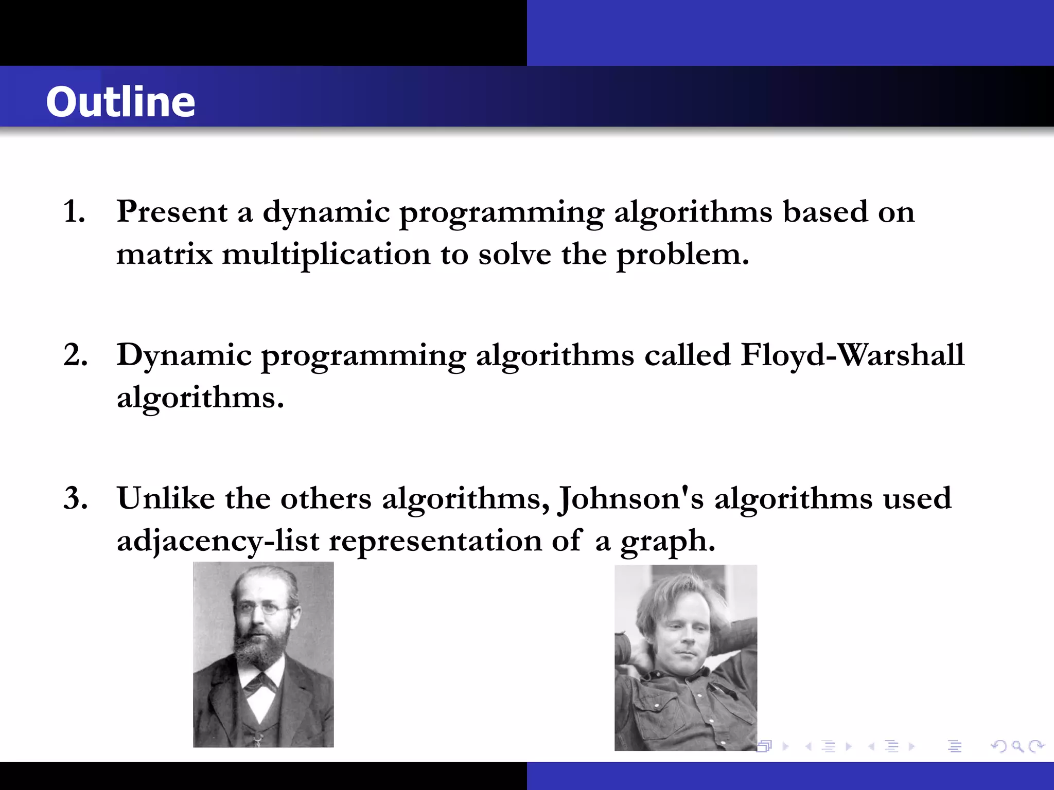
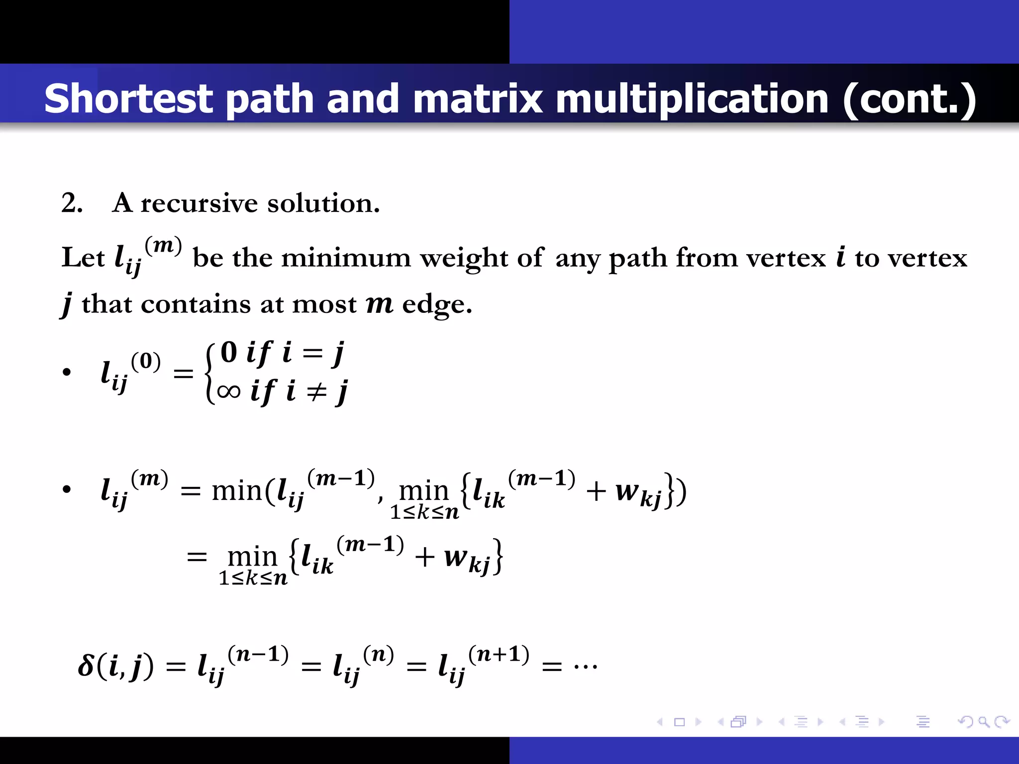
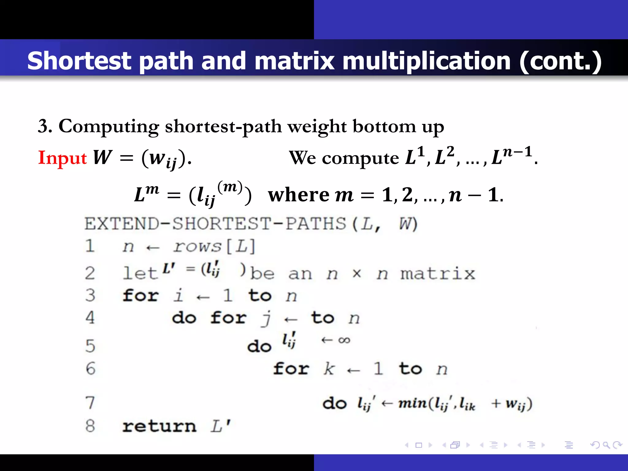
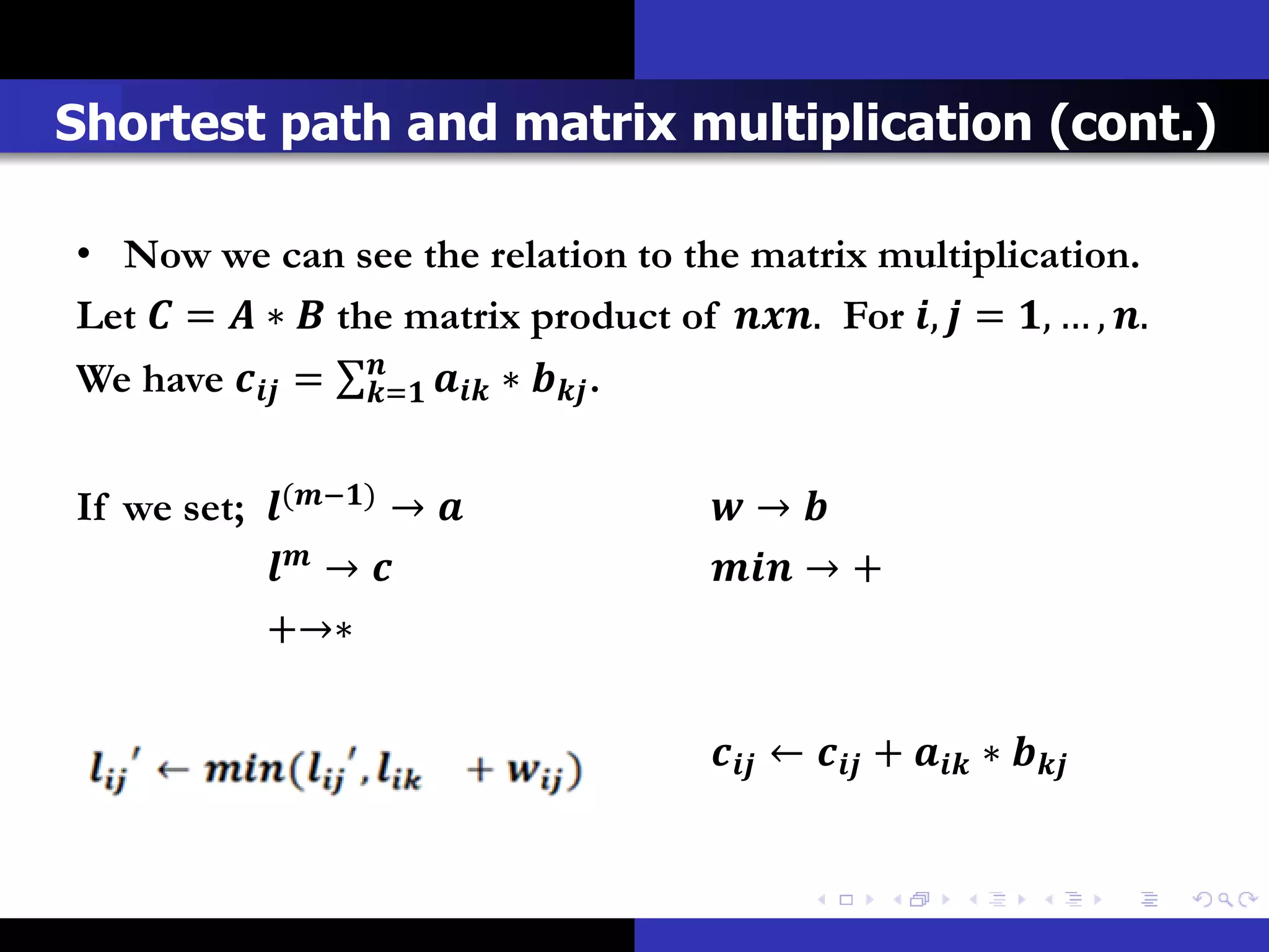
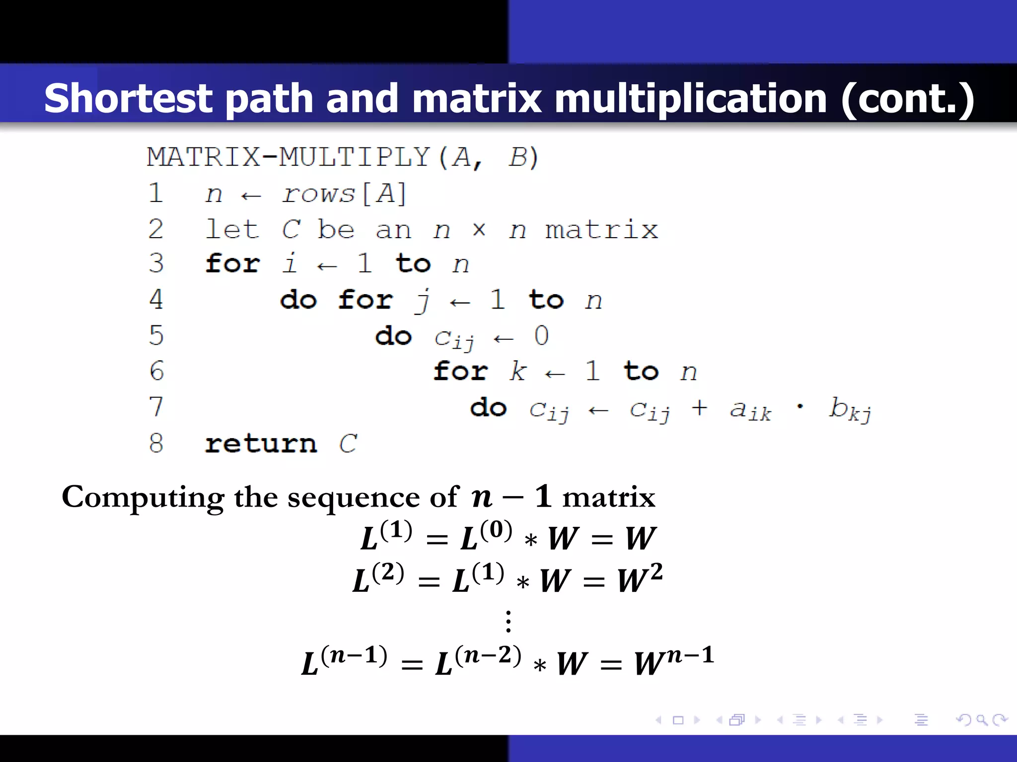
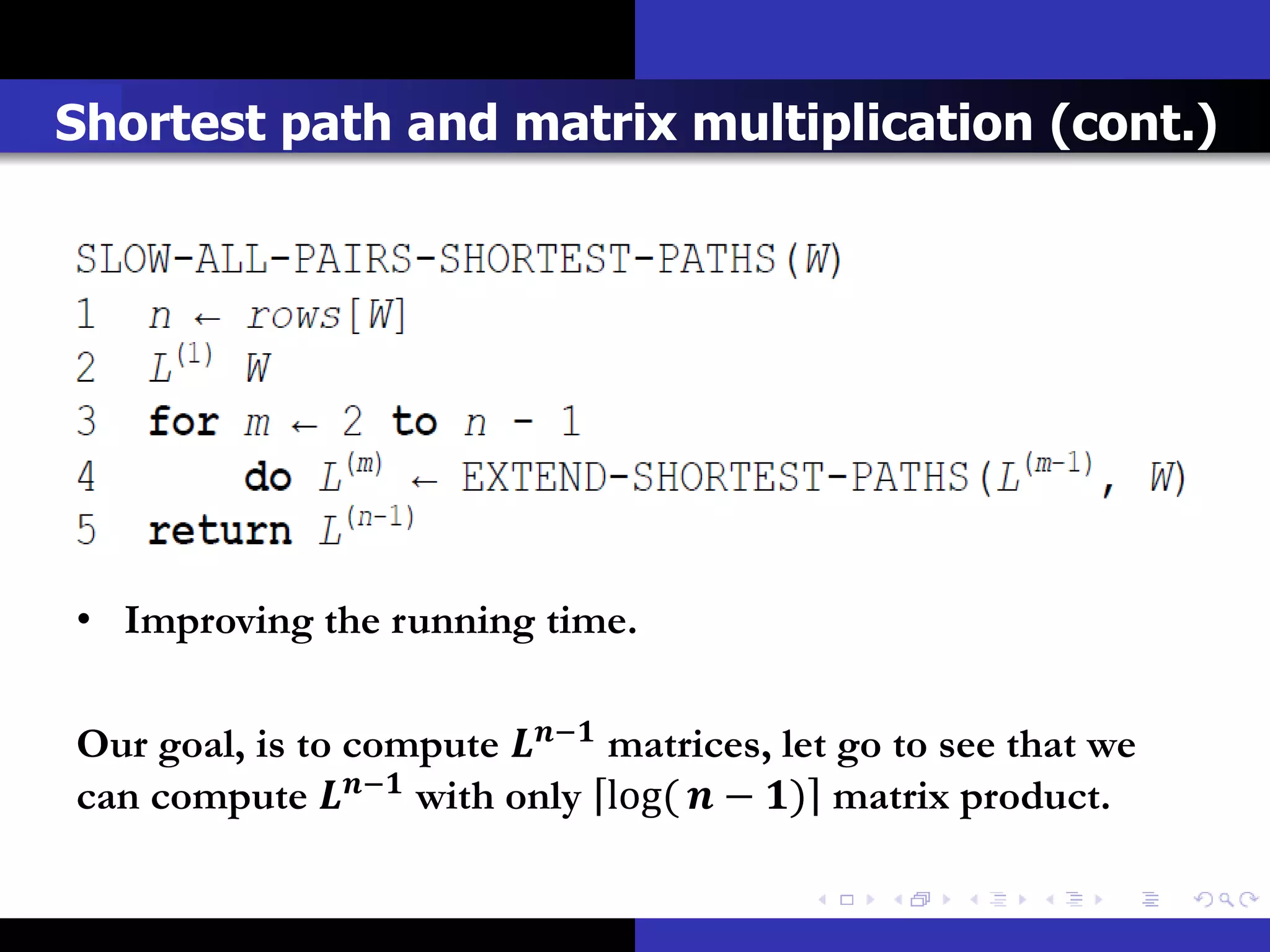
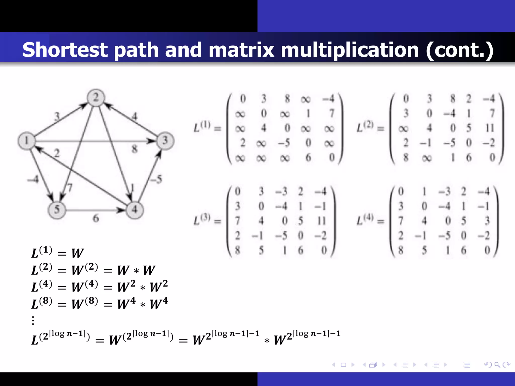
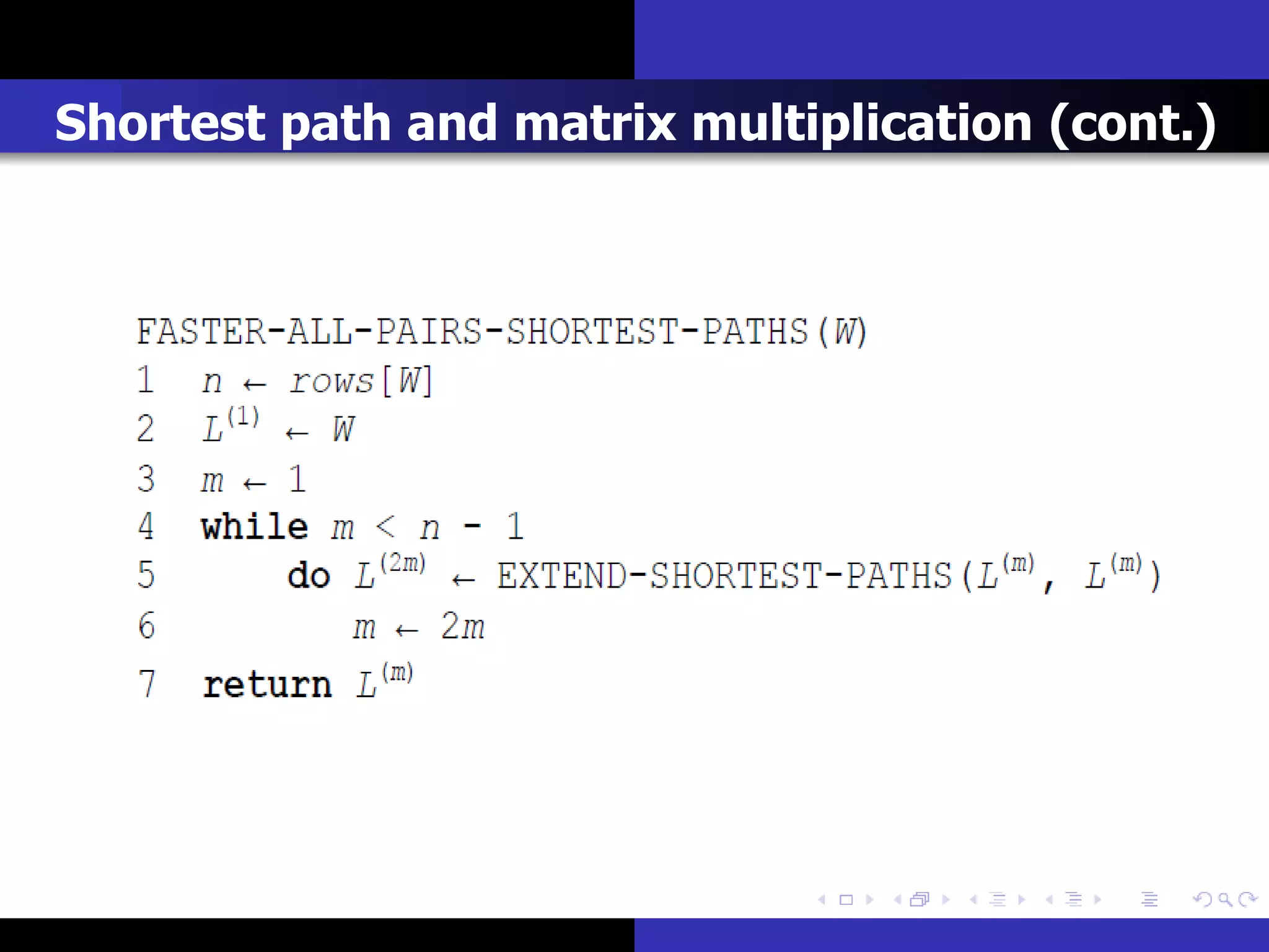
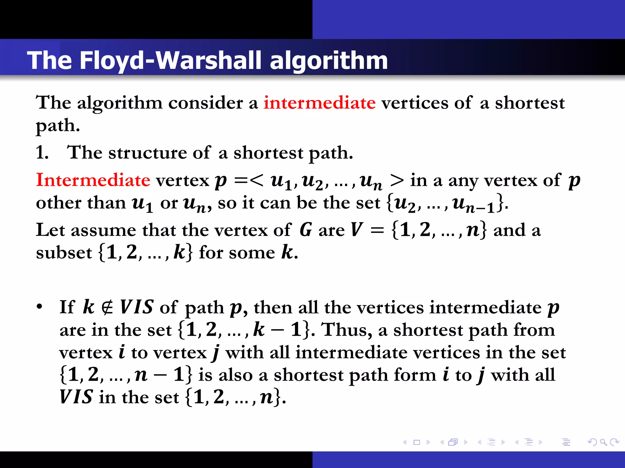
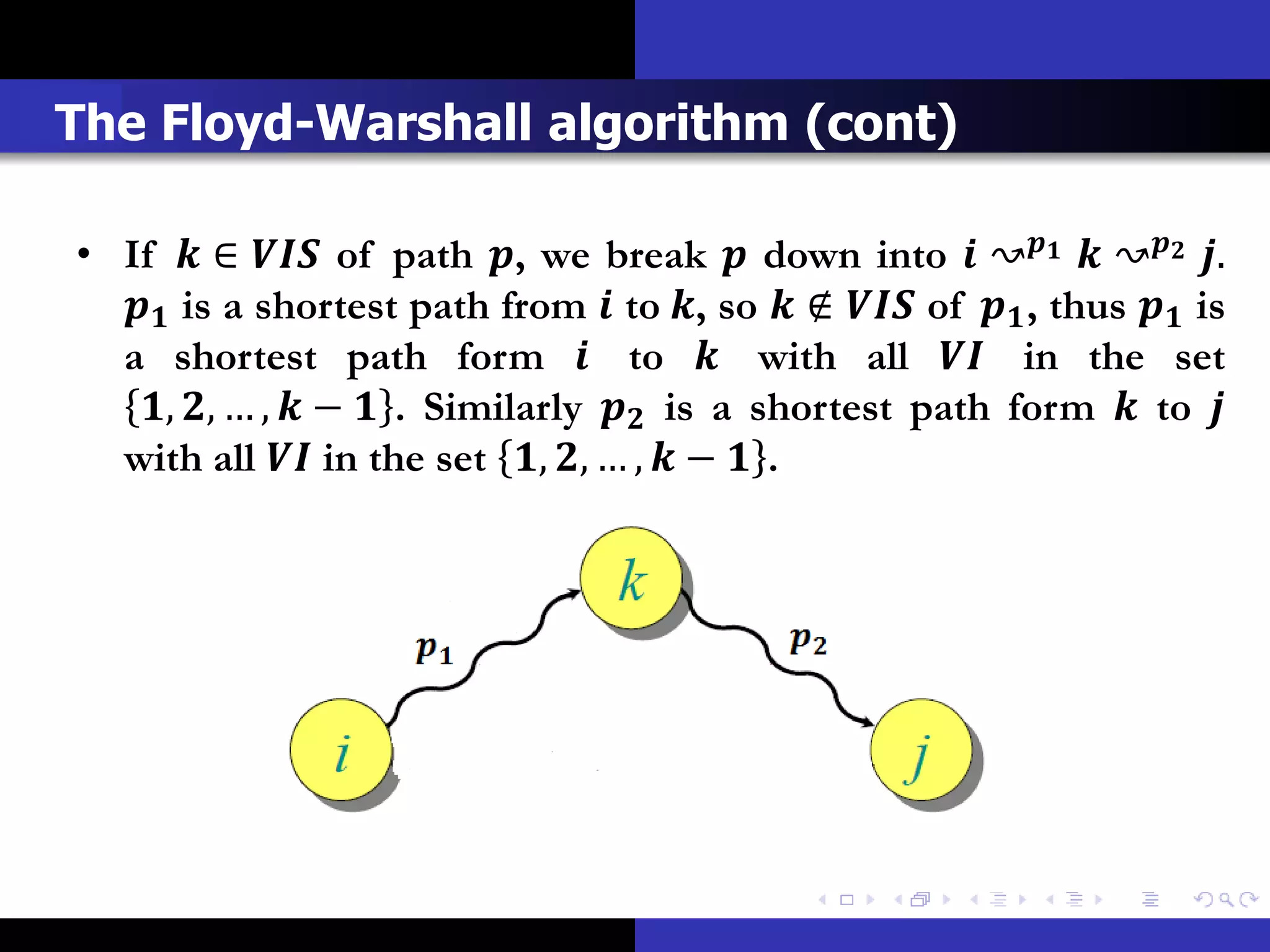
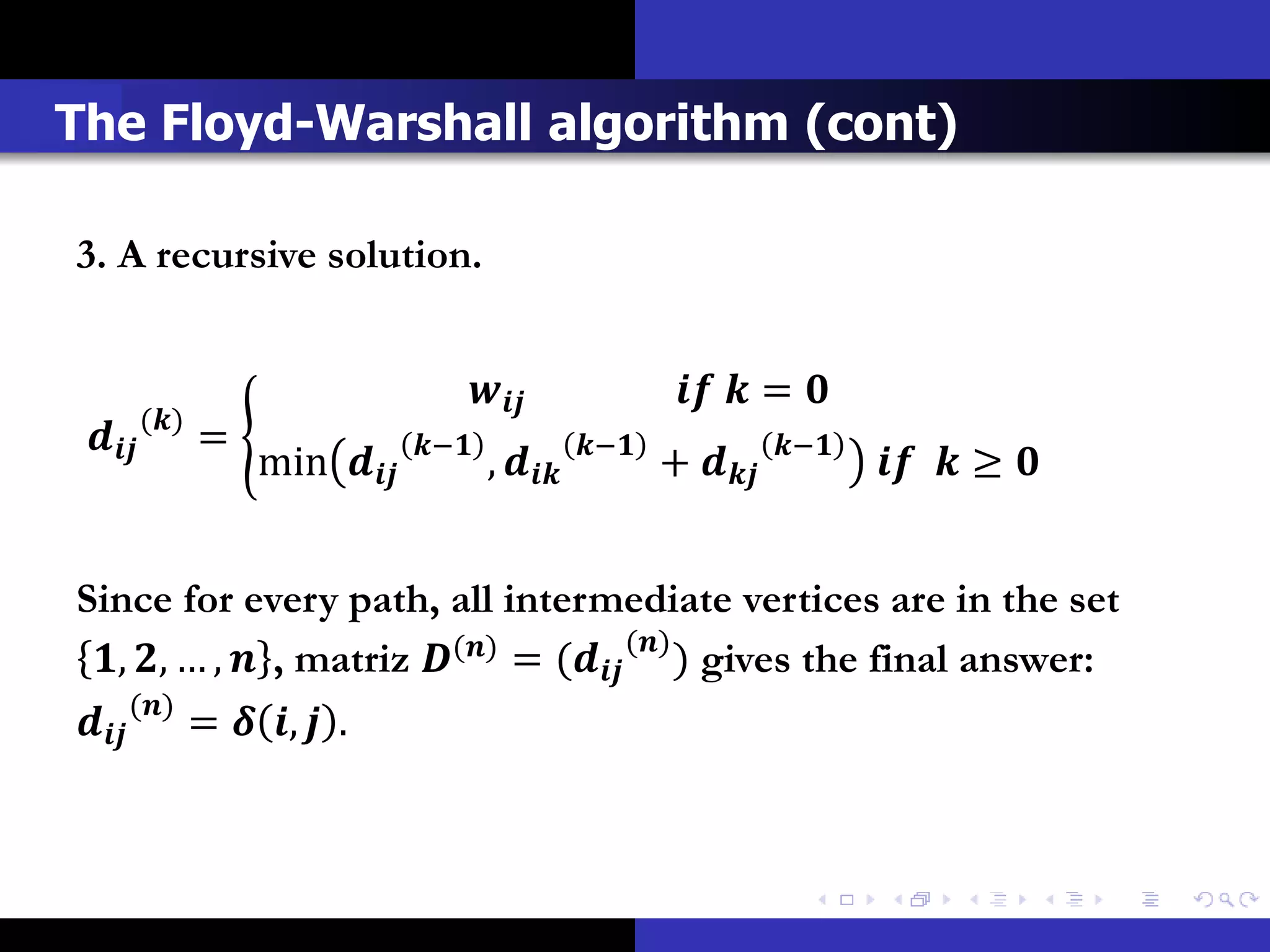
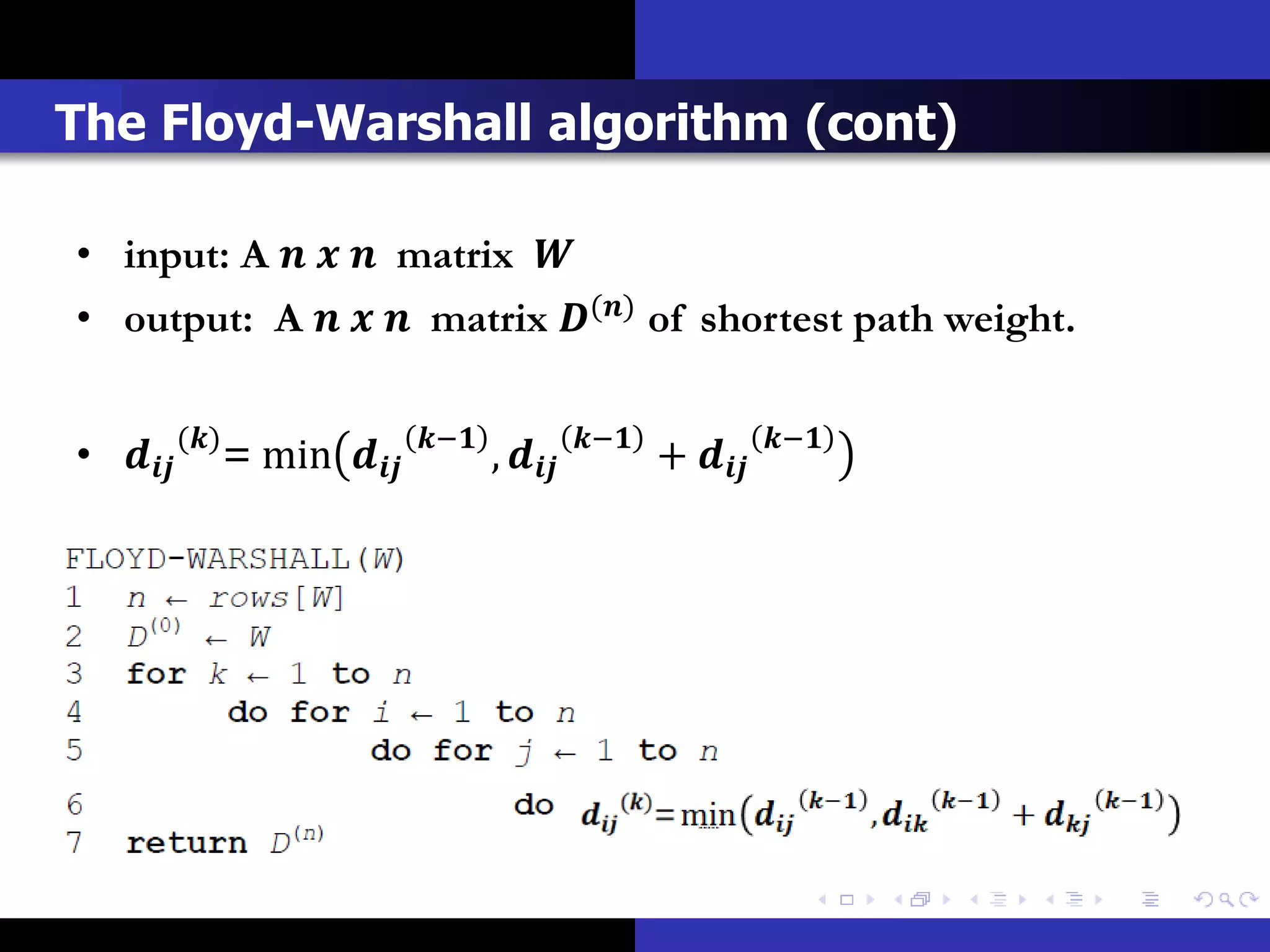
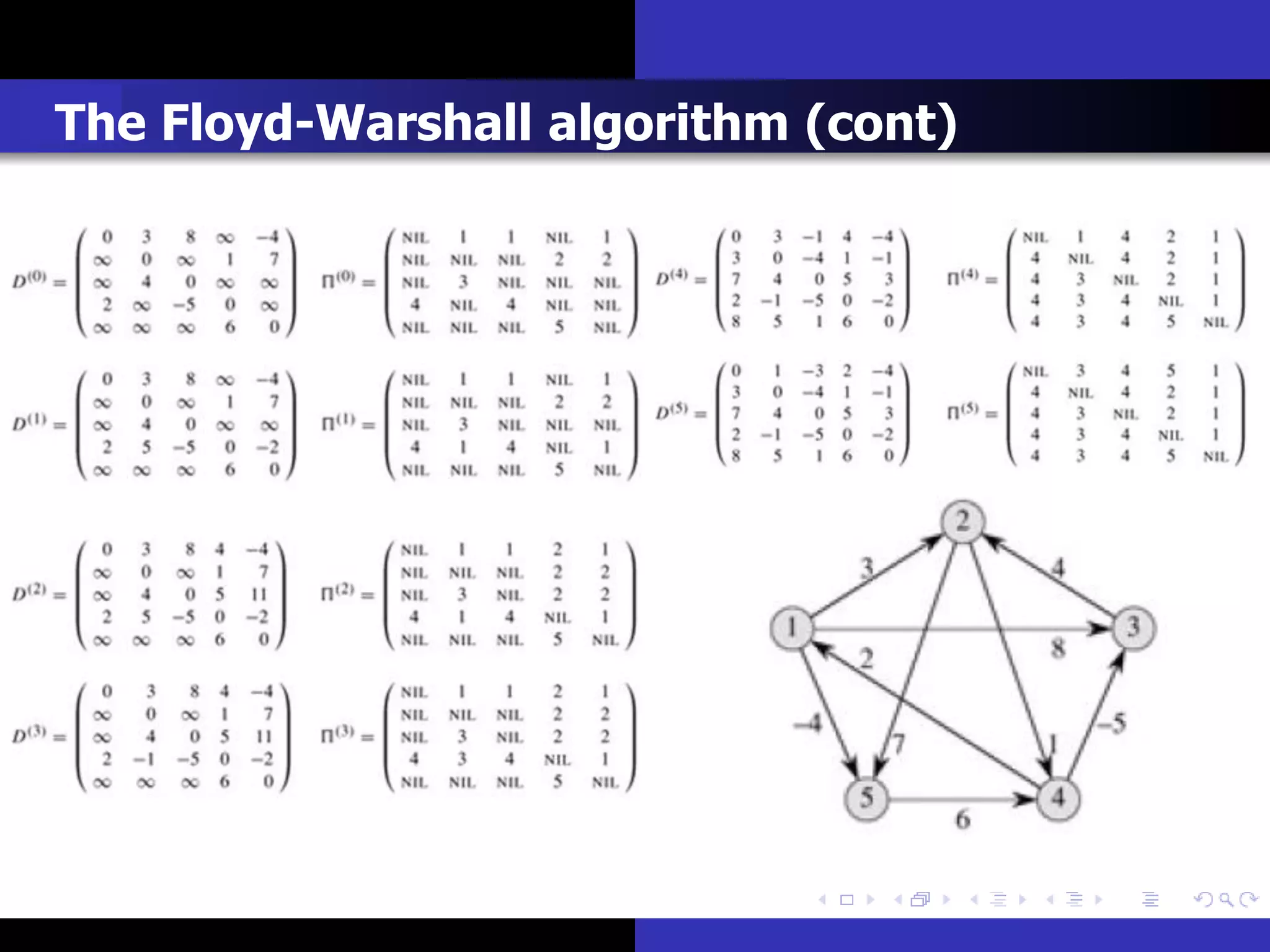
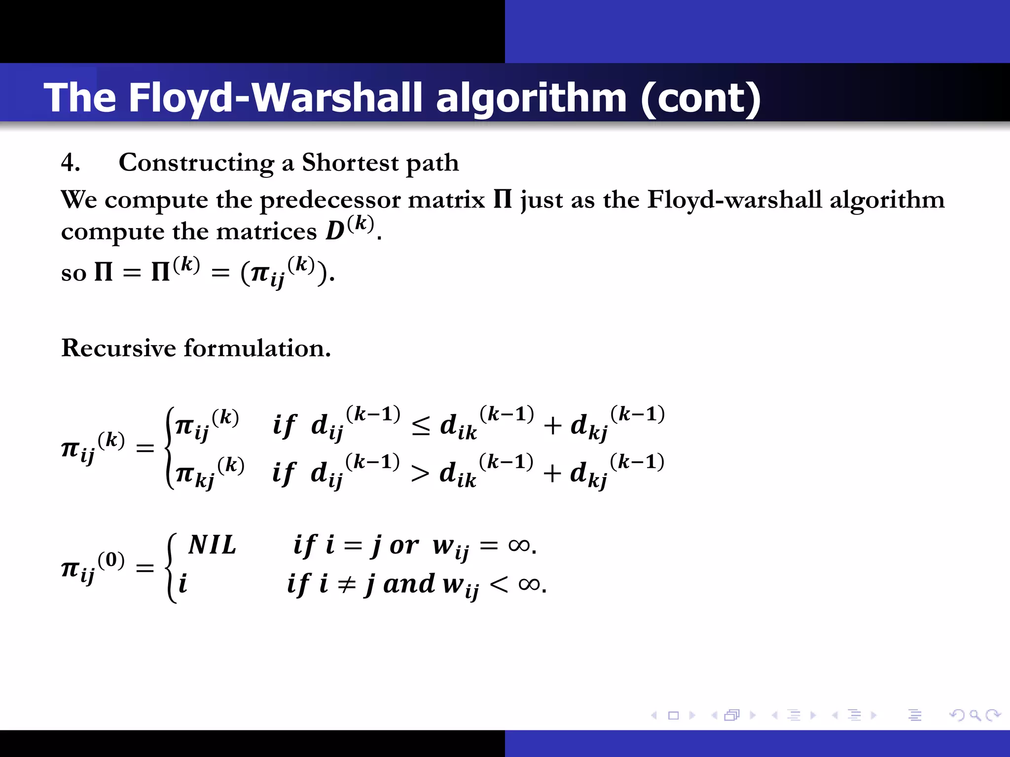
- Floyd-Warshall algorithm, which uses dynamic programming and matrix multiplication to compute the shortest paths matrix in O(V^3) time.
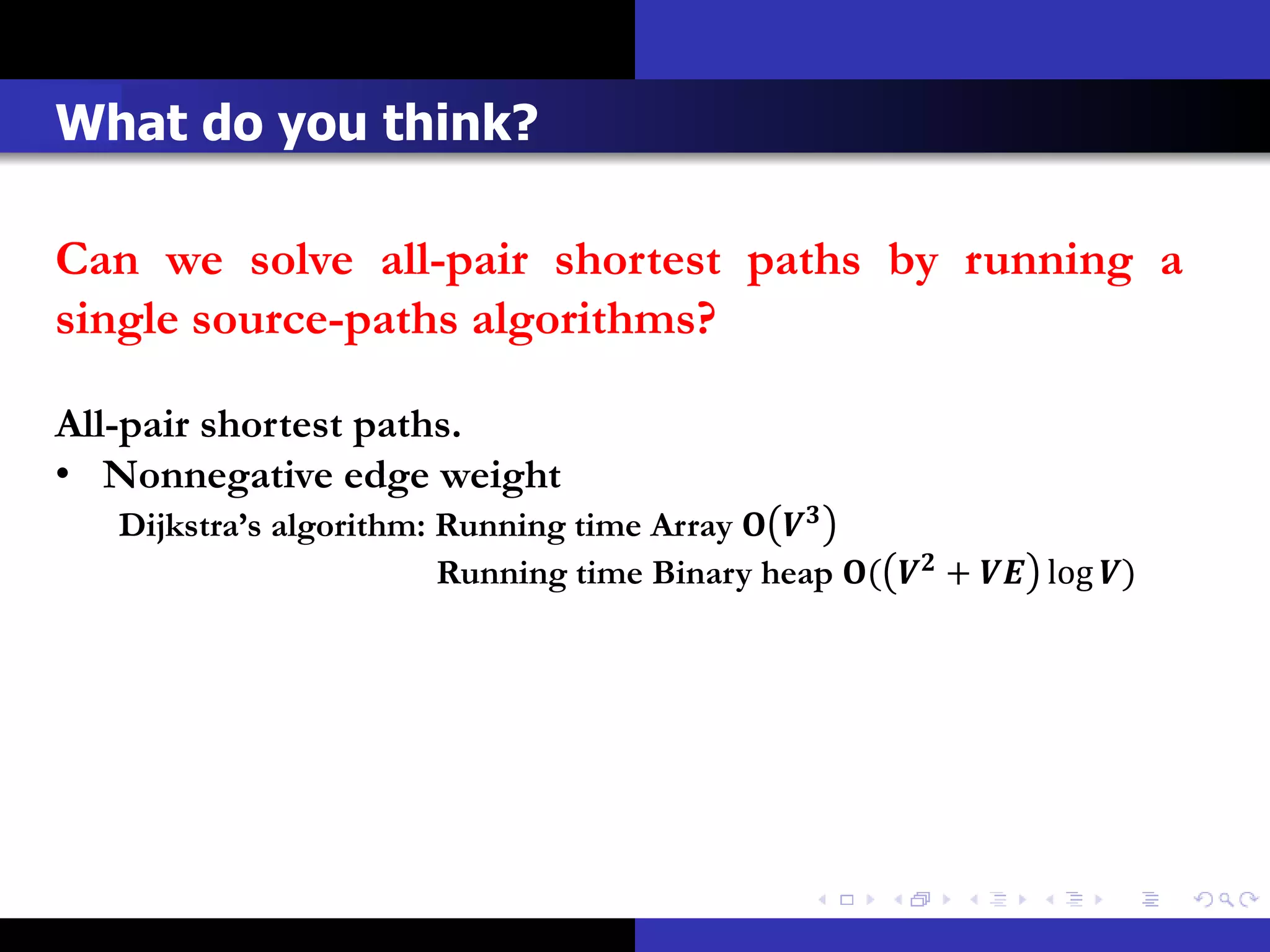
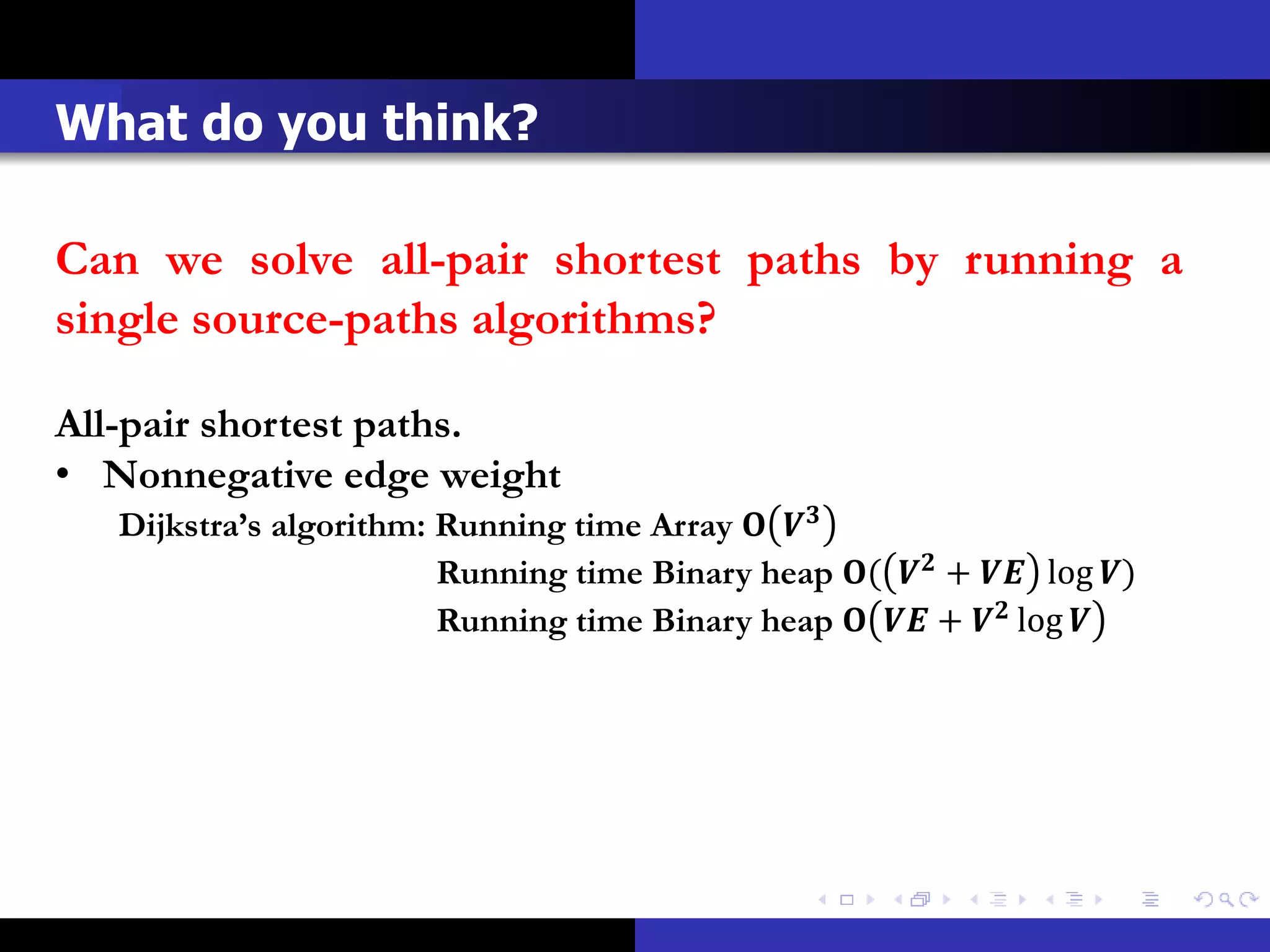
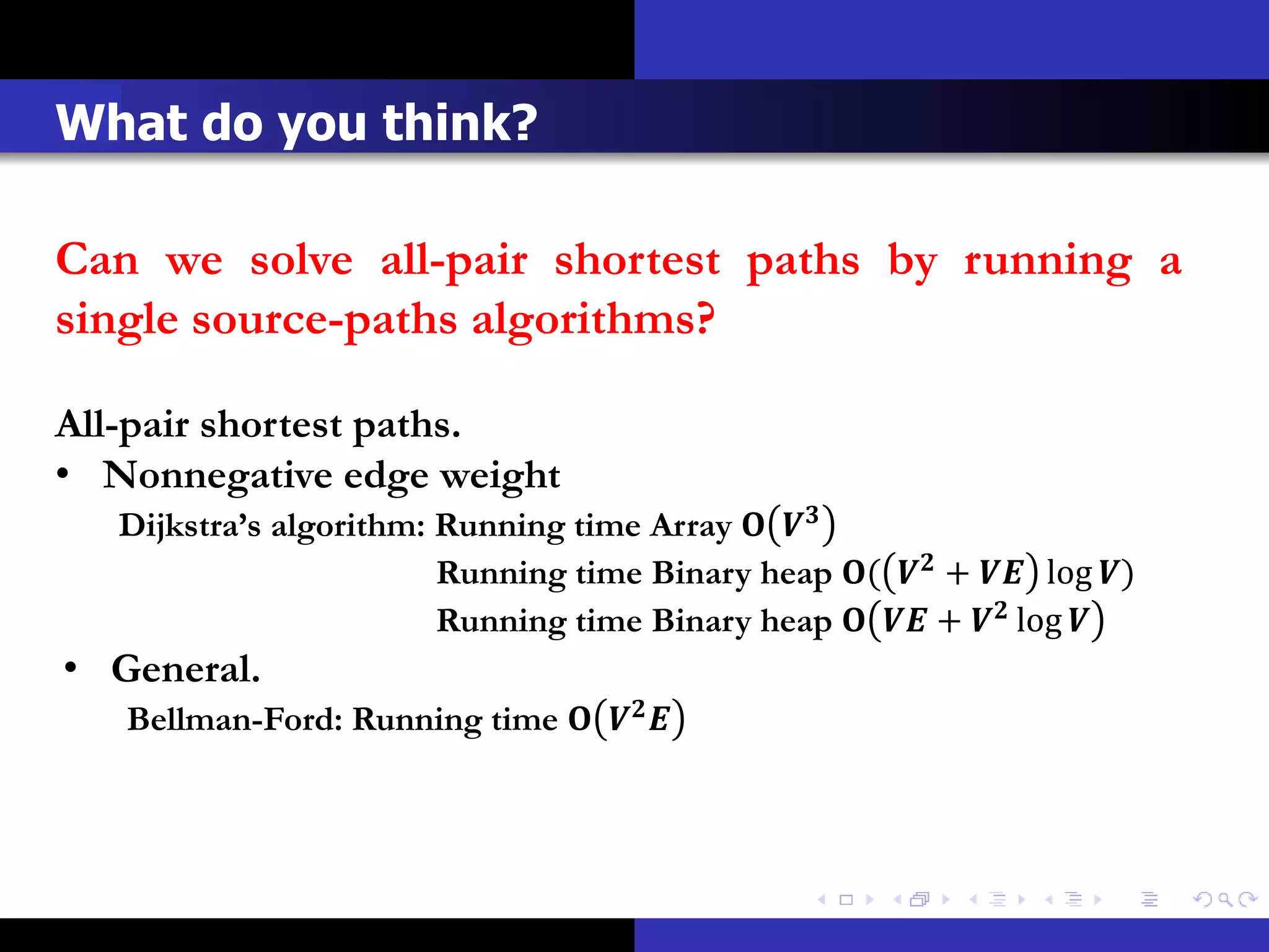
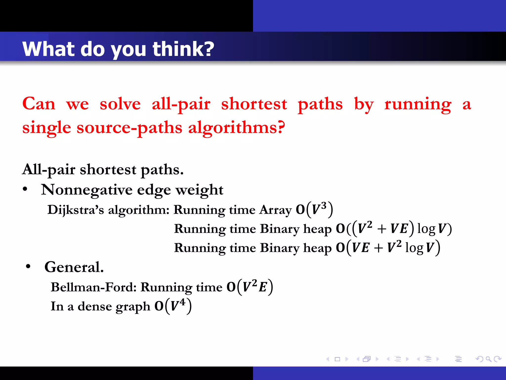
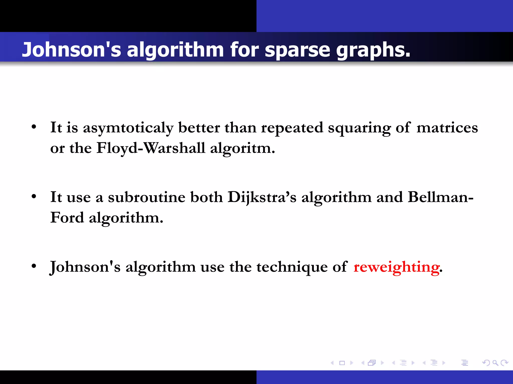
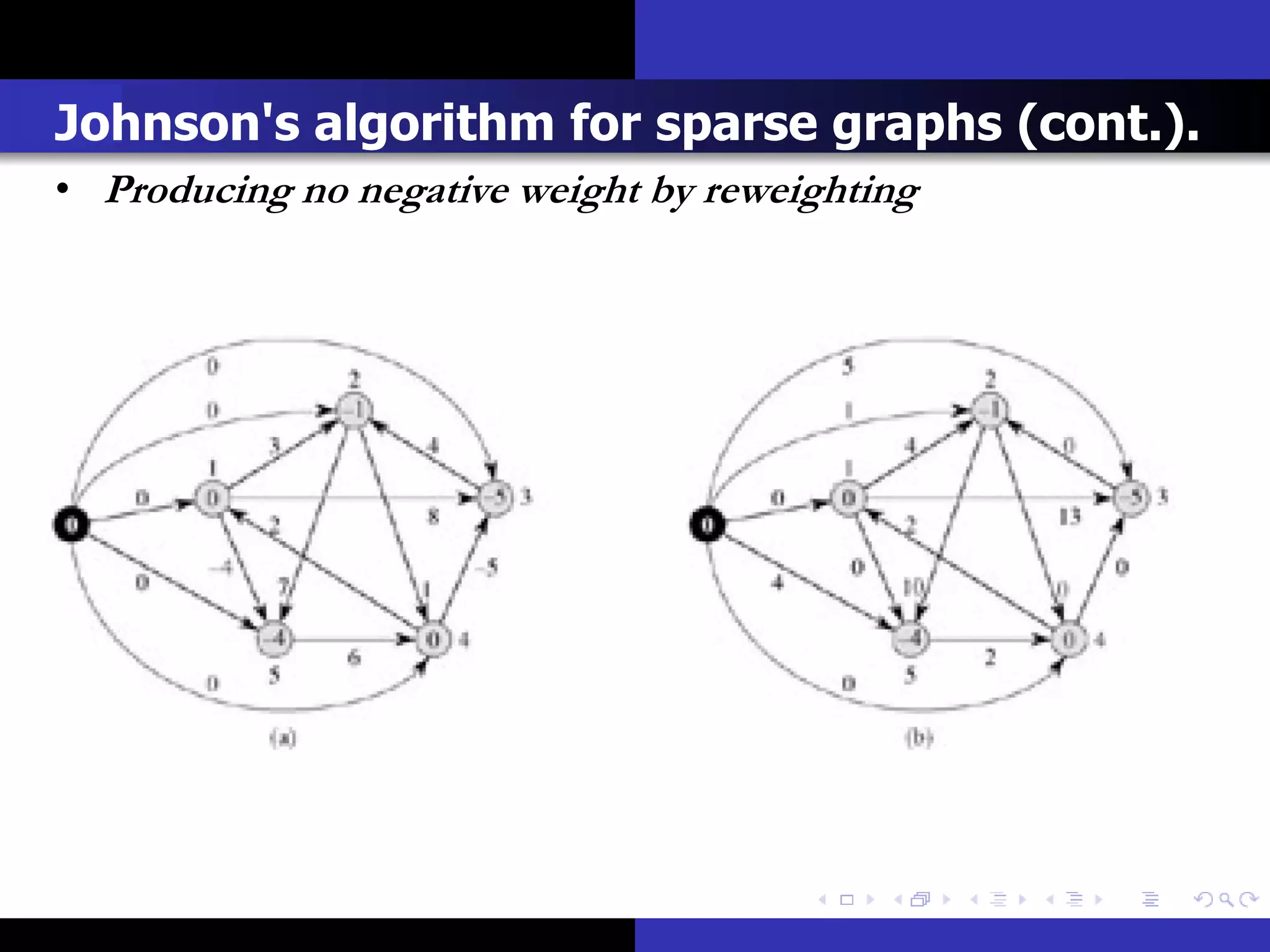
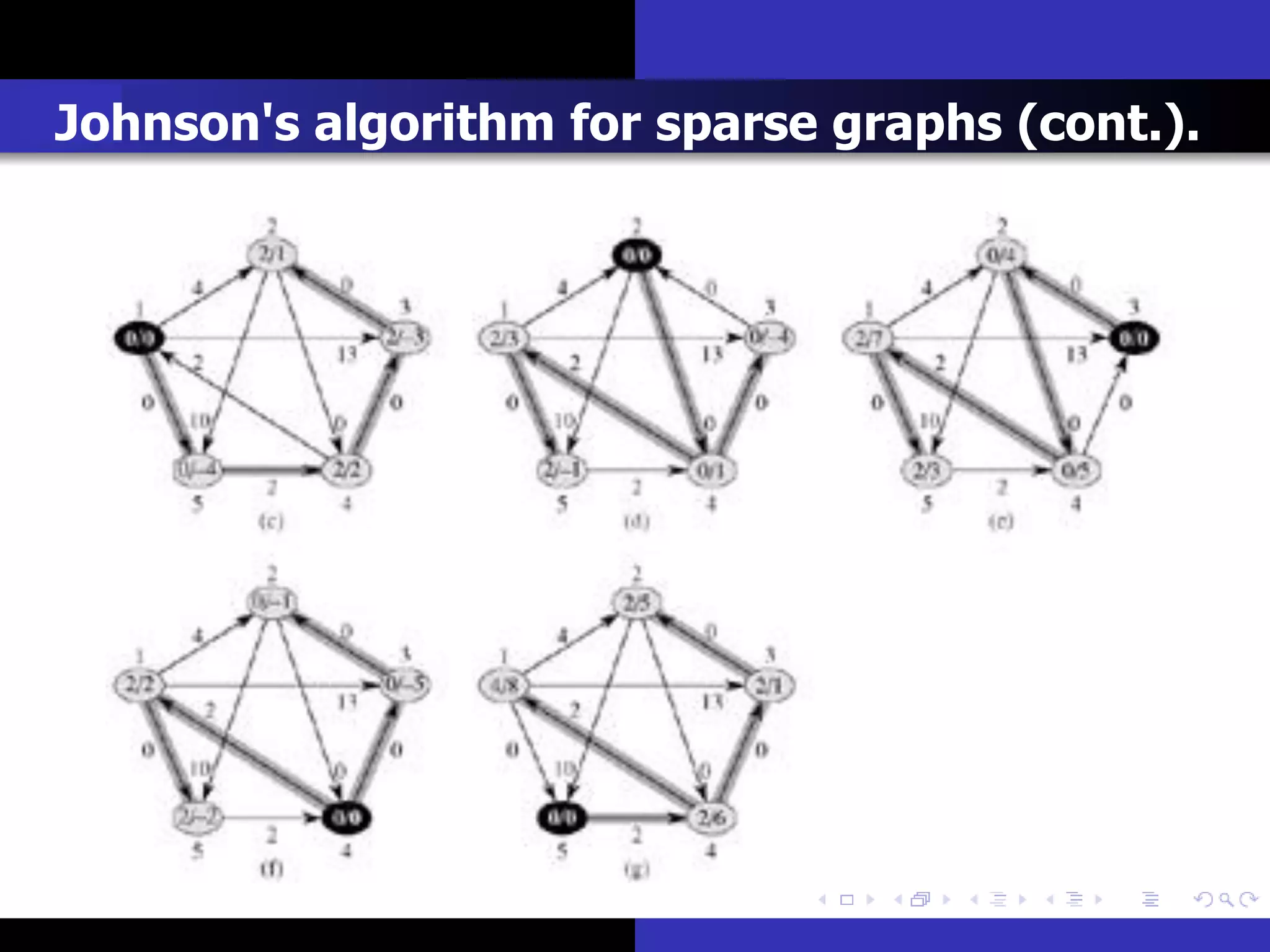
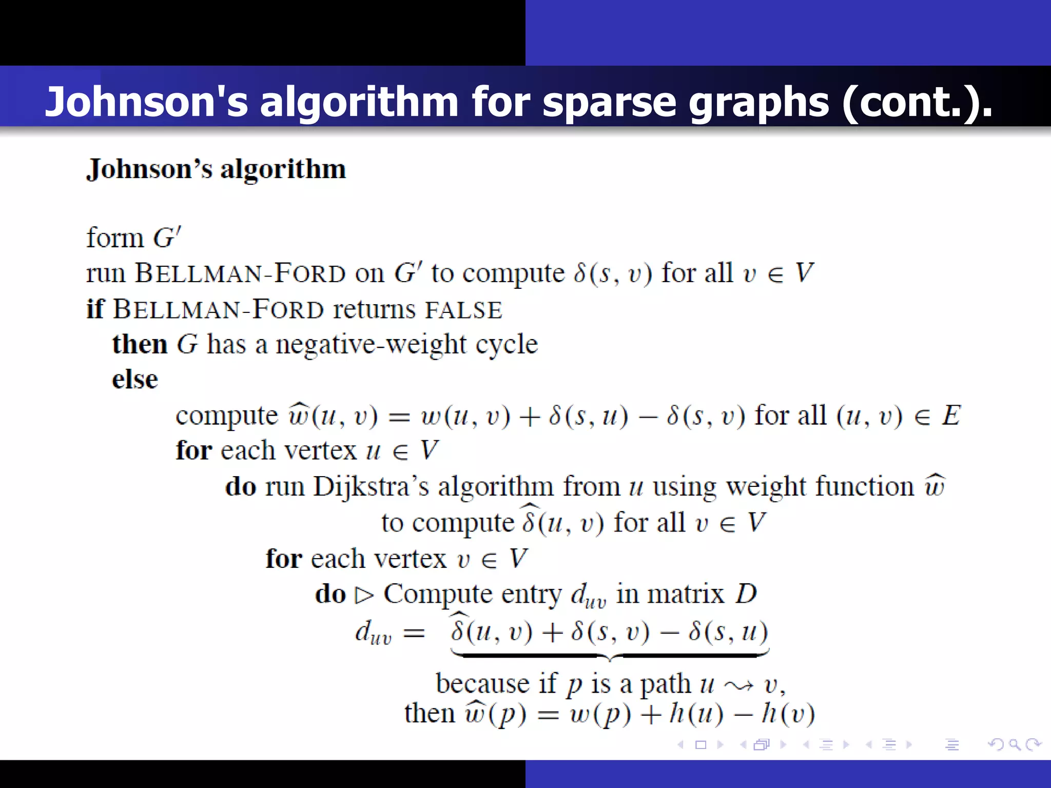
- Johnson's algorithm, which first reweights the graph to make all edge weights nonnegative, allowing it to use Dijkstra's algorithm repeatedly to solve the all-pairs shortest paths problem more efficiently for sparse graphs.
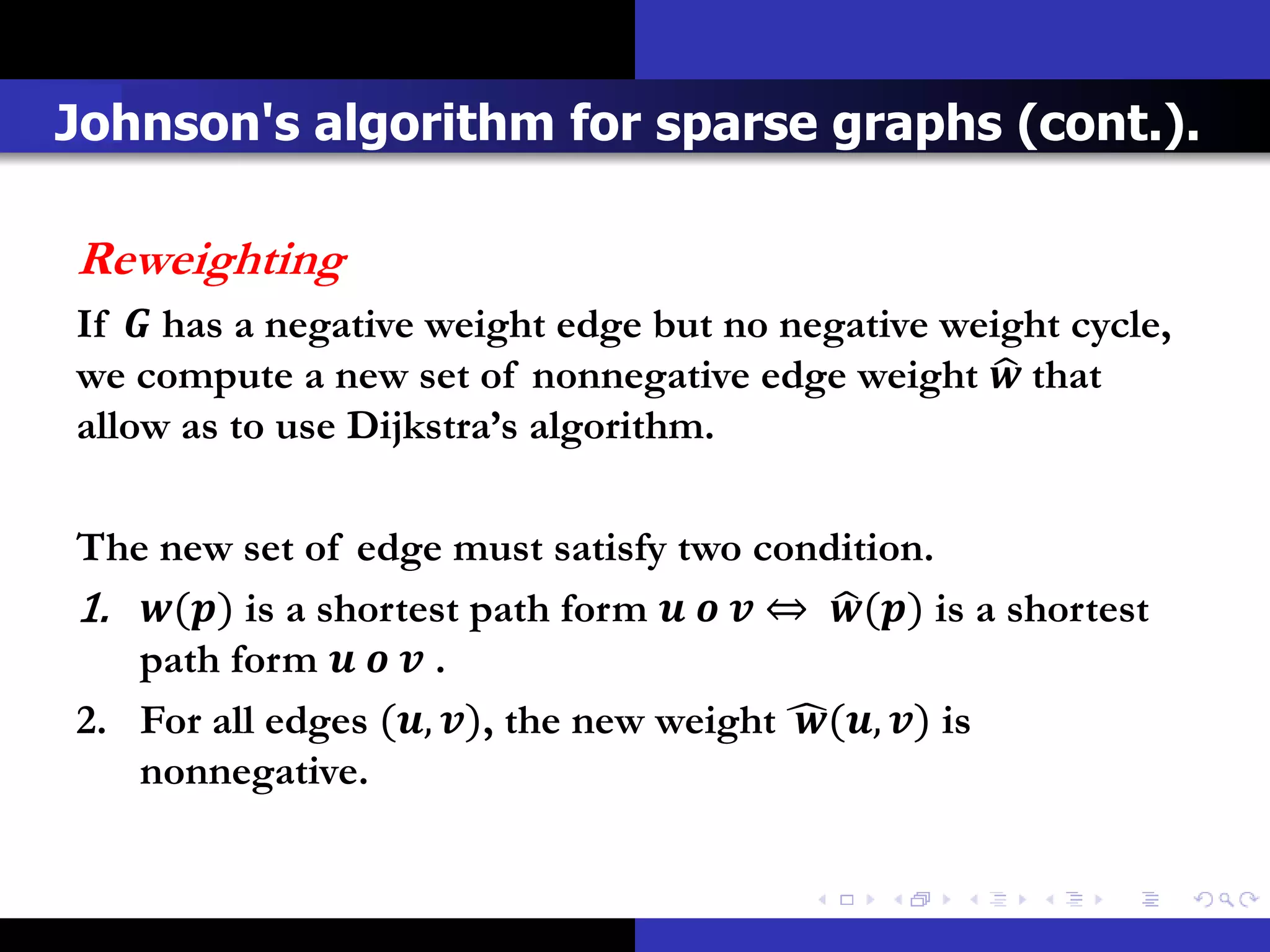
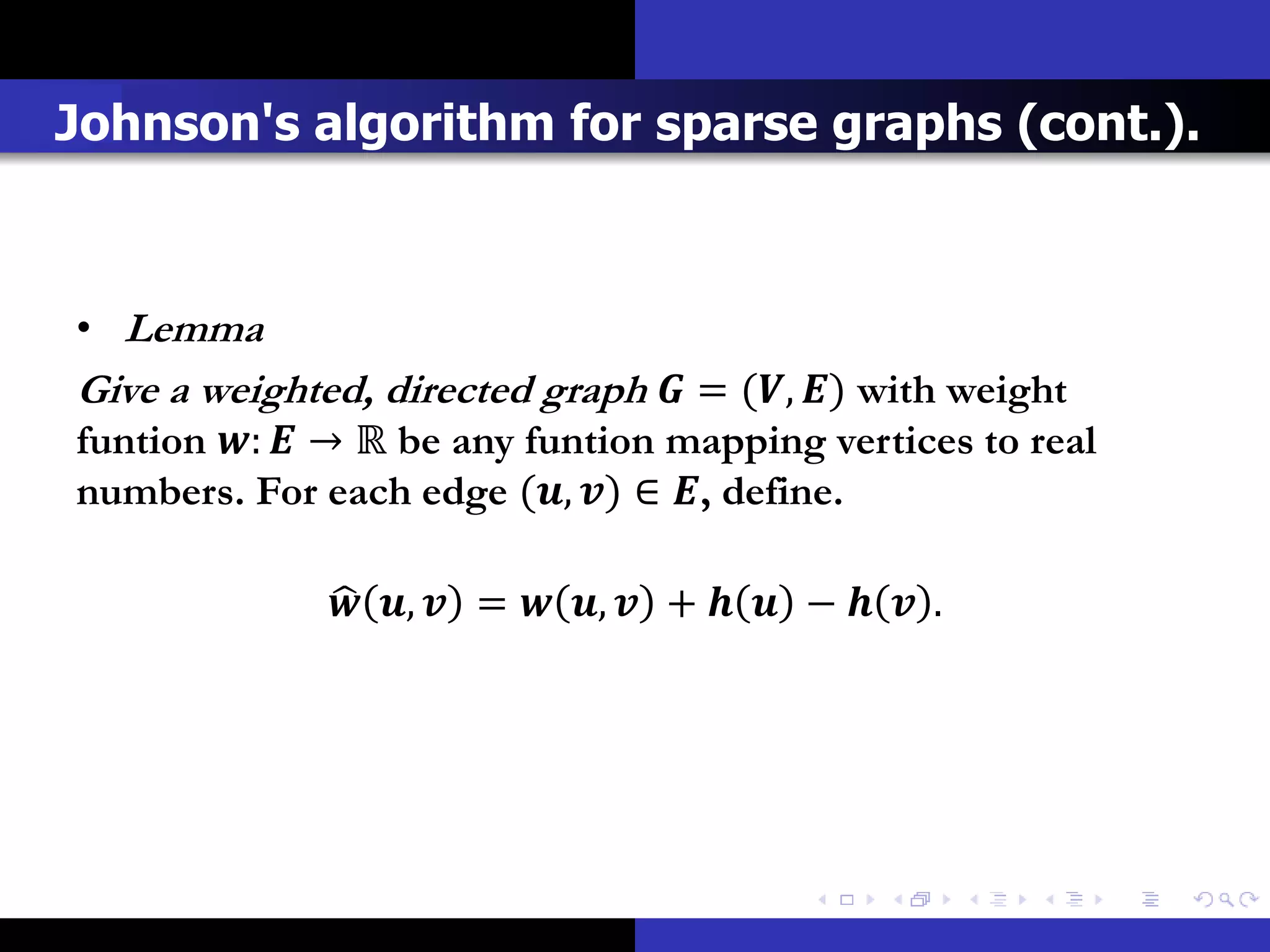
- Reweighting transforms the original graph in a way that preserves shortest path distances while ensuring nonnegative edge weights.


![Support, Monitoring, Continuous Improvement & Scaling Agentic Automation [3/3]](https://cdn.slidesharecdn.com/ss_thumbnails/agenticcommunityseries-day3-cfd-251120170304-ddef8112-thumbnail.jpg?width=640&height=640&fit=bounds)


