Downloaded 133 times


( 112
111
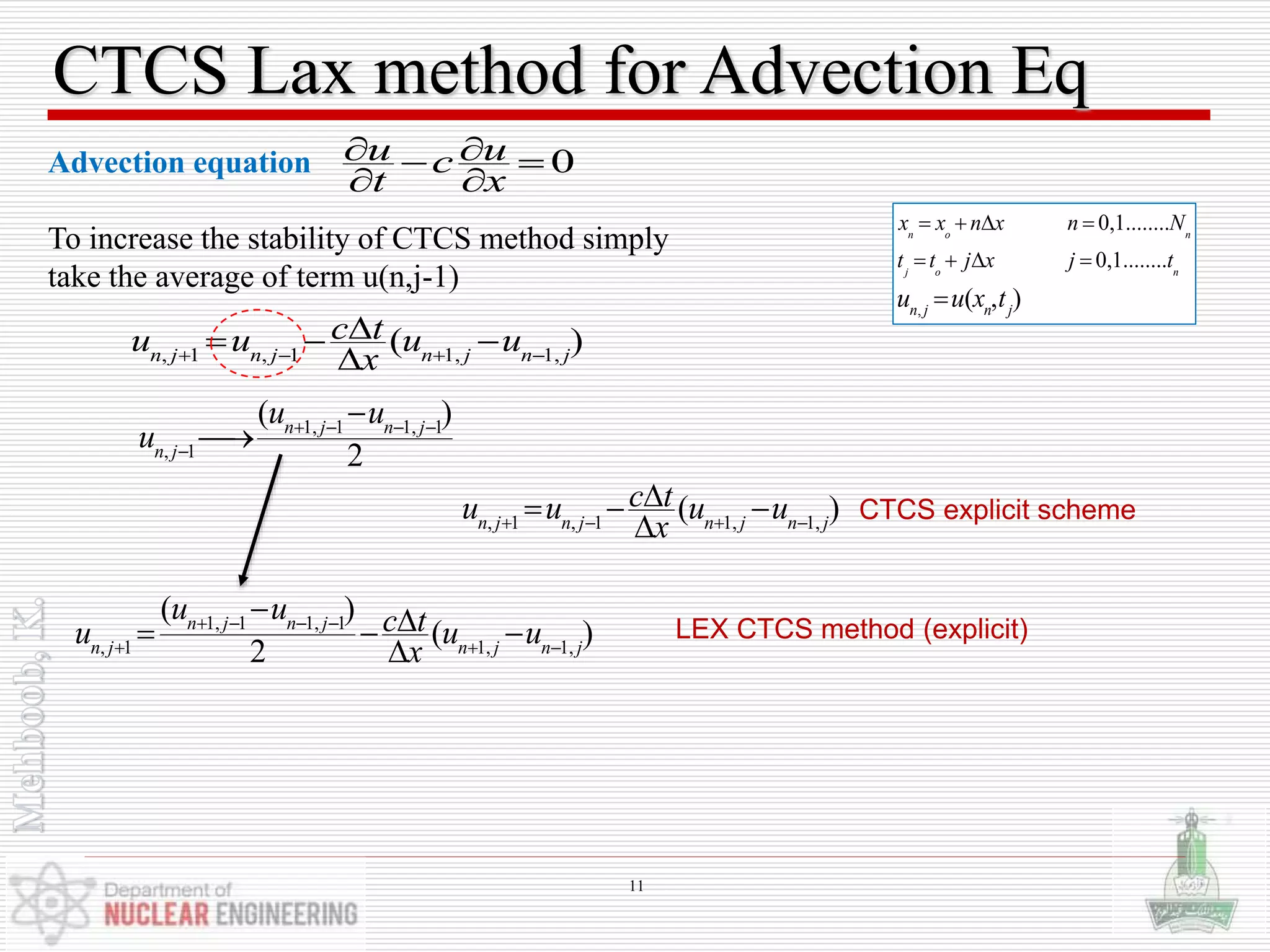
Replacement by average value from surrounding grid points
The resulting difference equation is
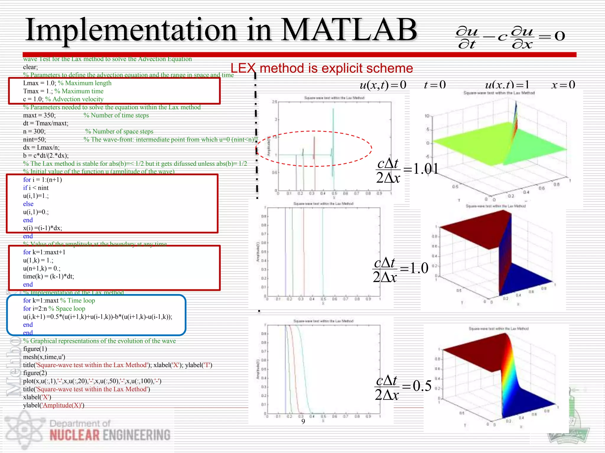
Courant condition for Lax method
4
1
2
x
tD
( Second-order accuracy in both time and space )
22](https://image.slidesharecdn.com/lecture18-19-20-180321201740/75/Computational-Method-to-Solve-the-Partial-Differential-Equations-PDEs-22-2048.jpg)
( 1
1
1
12
1111
Replacement by average value from surrounding grid points
The resulting difference equation is
Courant condition for Lax method
4
1
2
x
tD
( Second-order accuracy in both time and space )
23](https://image.slidesharecdn.com/lecture18-19-20-180321201740/75/Computational-Method-to-Solve-the-Partial-Differential-Equations-PDEs-23-2048.jpg)
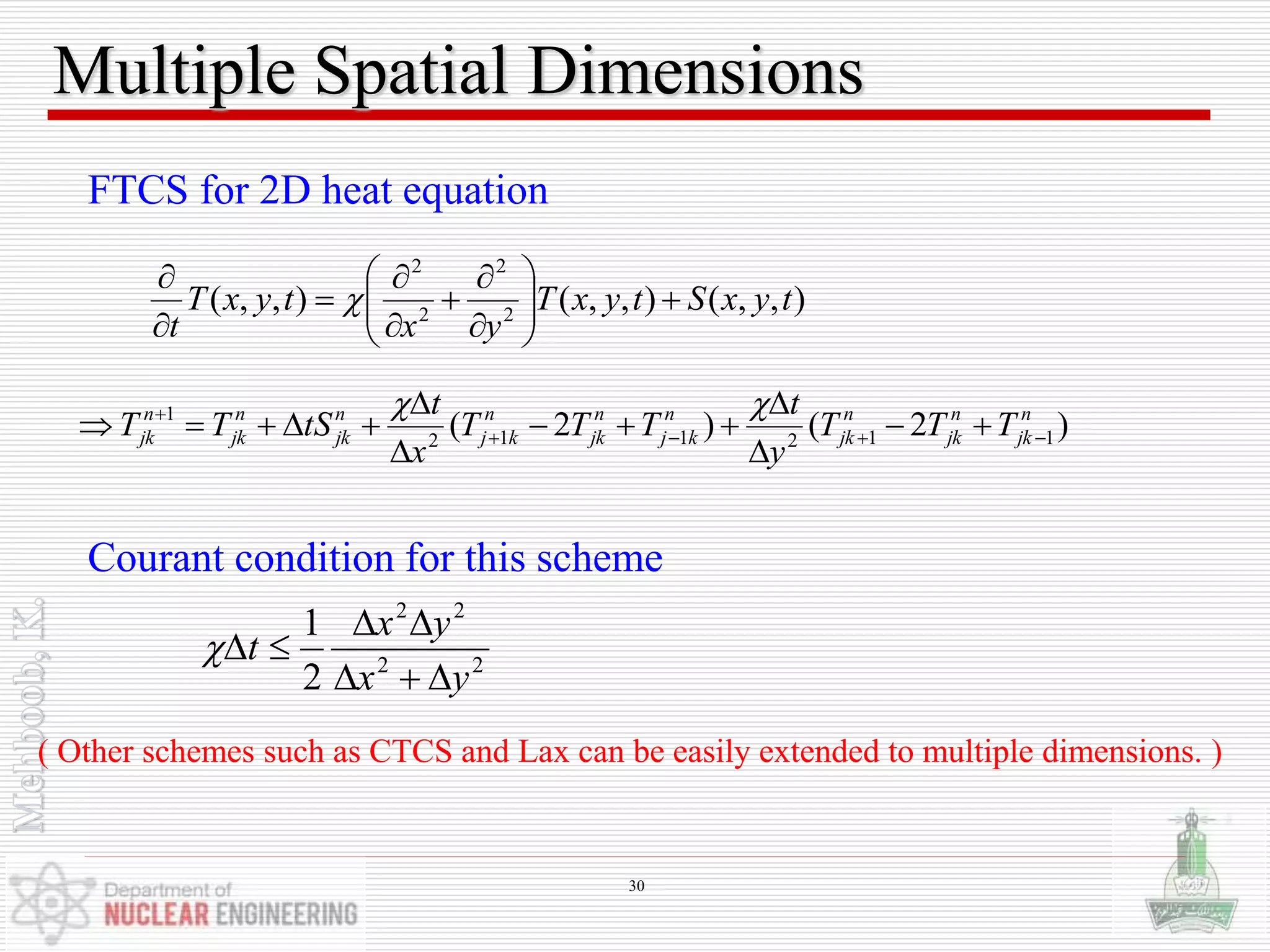
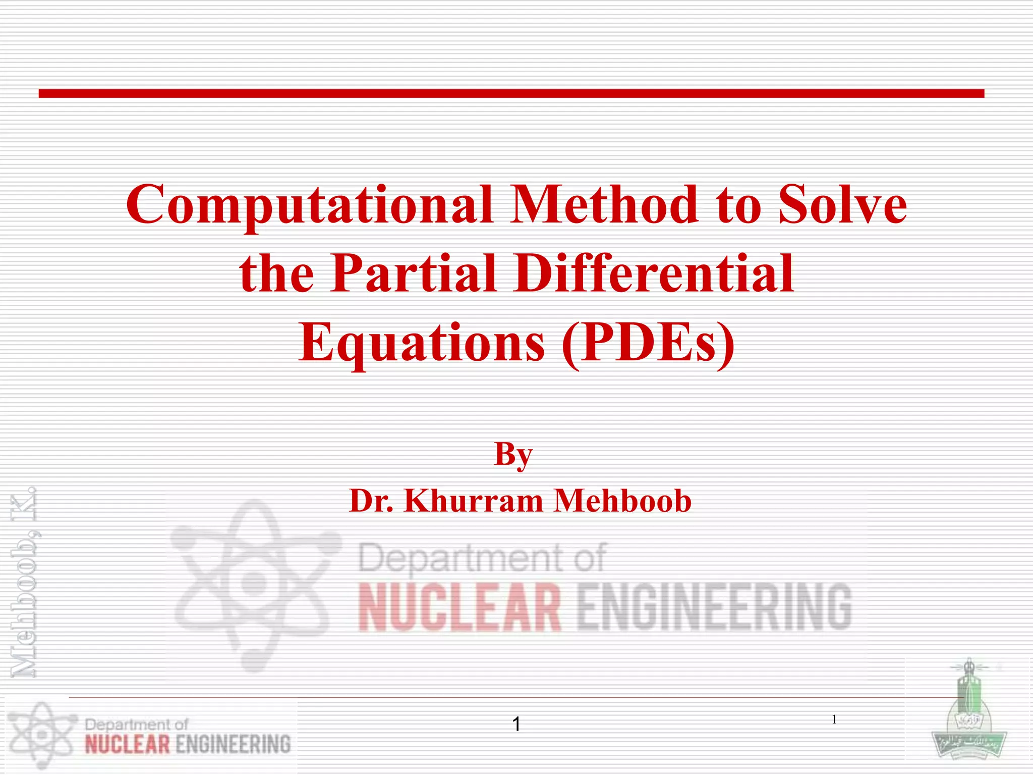
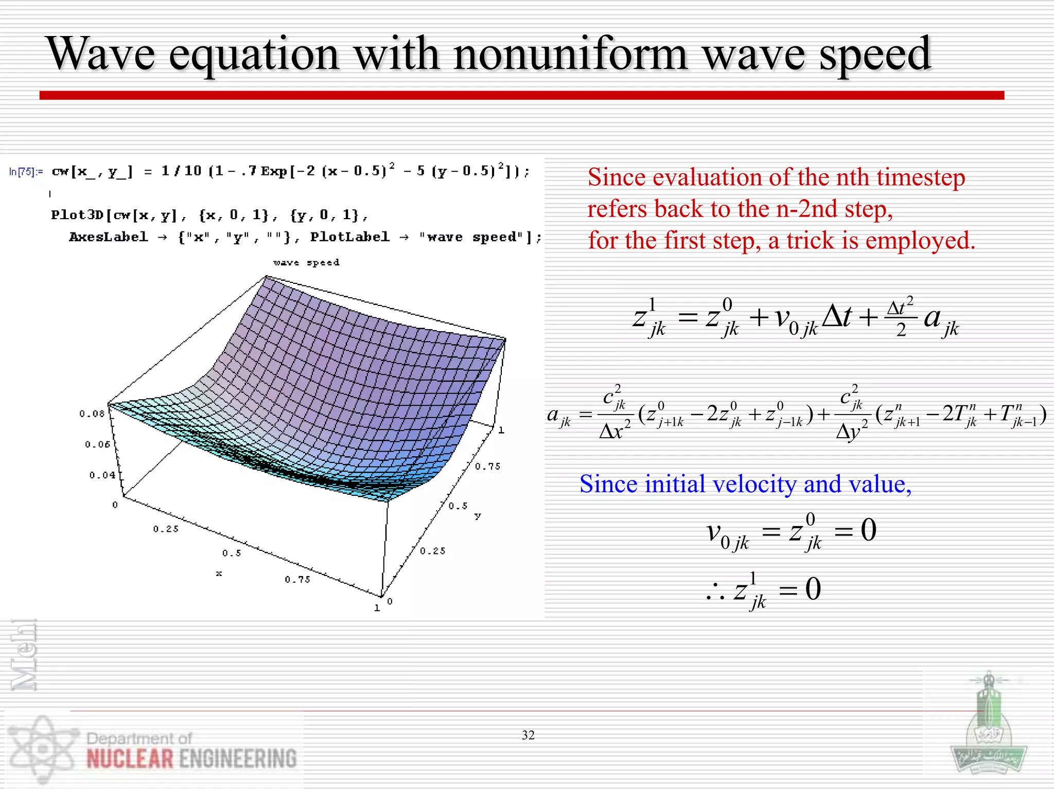
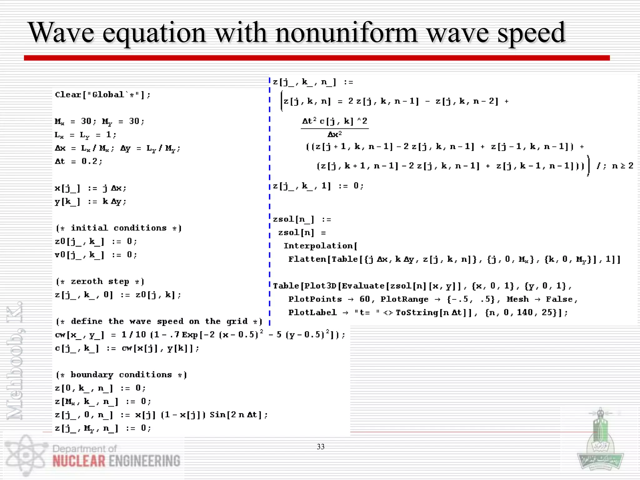
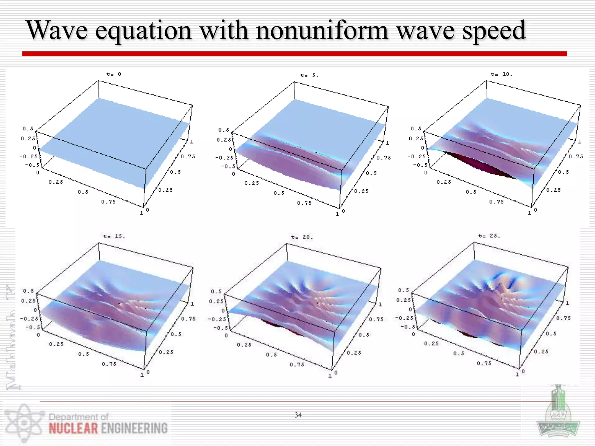
![Wave equation with nonuniform wave speed
),,(),(),,( 2
2
2
2
2
2
2
tyxz
yx
yxctyxz
t
2D wave equation
0
),()0,,(),,()0,,(
00
00
vz
yxvyxzyxzyxz
txxtxz
txztyztyz
2sin)1(),0,(
,0),1,(),,1(),,0(
Initial condition :
Boundary
condition :
])5.0(5)5.0(2exp[7.01),( 22
10
1
yxyxcWave speed :
)2()2(2 112
22
112
22
11 n
jk
n
jk
n
jk
jkn
kj
n
jk
n
kj
jkn
jk
n
jk
n
jk TTz
y
tc
zzz
x
tc
zzz
CTCS method for the wave equation :
)(
2
1
2
22
yxfor
tc
Courant condition :
31](https://image.slidesharecdn.com/lecture18-19-20-180321201740/75/Computational-Method-to-Solve-the-Partial-Differential-Equations-PDEs-31-2048.jpg)


( 112
111
Replacement by average value from surrounding grid points
The resulting difference equation is
Courant condition for Lax method
4
1
2
x
tD
( Second-order accuracy in both time and space )
22](https://crownmelresort.com/image.slidesharecdn.com/lecture18-19-20-180321201740/75/Computational-Method-to-Solve-the-Partial-Differential-Equations-PDEs-22-2048.jpg)
( 1
1
1
12
1111
Replacement by average value from surrounding grid points
The resulting difference equation is
Courant condition for Lax method
4
1
2
x
tD
( Second-order accuracy in both time and space )
23](https://crownmelresort.com/image.slidesharecdn.com/lecture18-19-20-180321201740/75/Computational-Method-to-Solve-the-Partial-Differential-Equations-PDEs-23-2048.jpg)


![Wave equation with nonuniform wave speed
),,(),(),,( 2
2
2
2
2
2
2
tyxz
yx
yxctyxz
t
2D wave equation
0
),()0,,(),,()0,,(
00
00
vz
yxvyxzyxzyxz
txxtxz
txztyztyz
2sin)1(),0,(
,0),1,(),,1(),,0(
Initial condition :
Boundary
condition :
])5.0(5)5.0(2exp[7.01),( 22
10
1
yxyxcWave speed :
)2()2(2 112
22
112
22
11 n
jk
n
jk
n
jk
jkn
kj
n
jk
n
kj
jkn
jk
n
jk
n
jk TTz
y
tc
zzz
x
tc
zzz
CTCS method for the wave equation :
)(
2
1
2
22
yxfor
tc
Courant condition :
31](https://crownmelresort.com/image.slidesharecdn.com/lecture18-19-20-180321201740/75/Computational-Method-to-Solve-the-Partial-Differential-Equations-PDEs-31-2048.jpg)


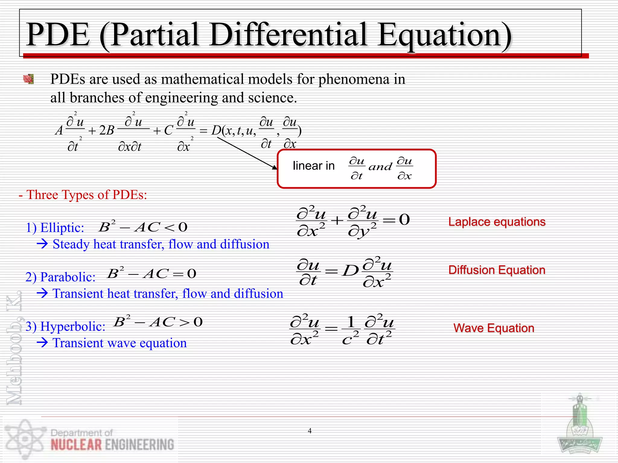
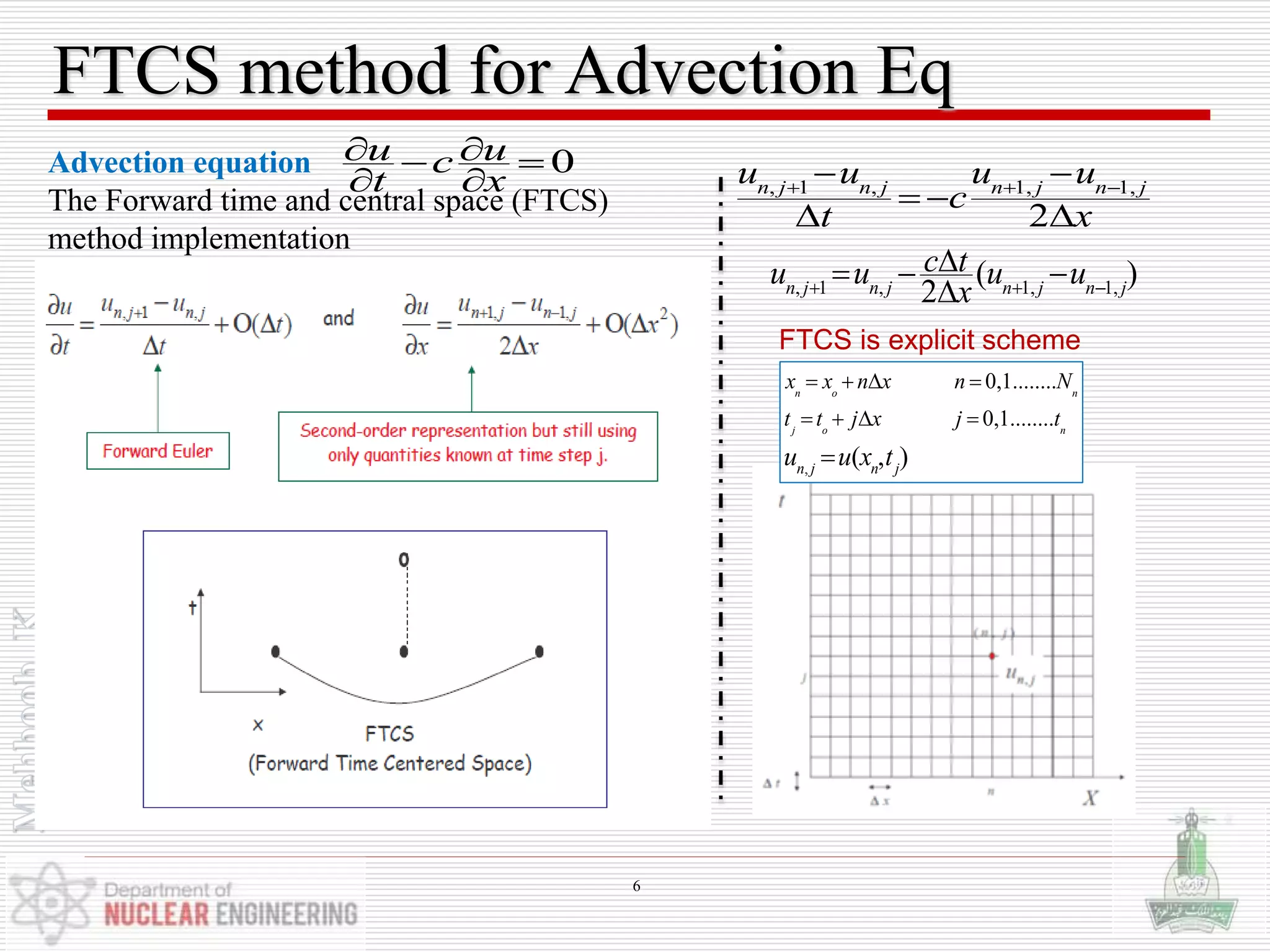
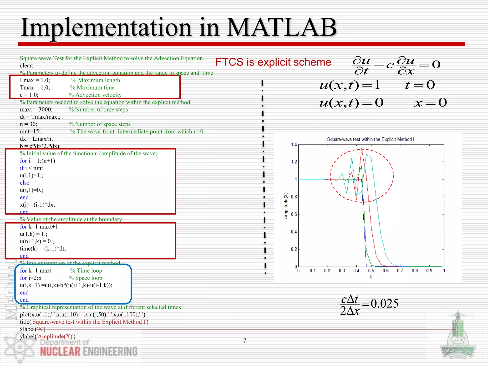
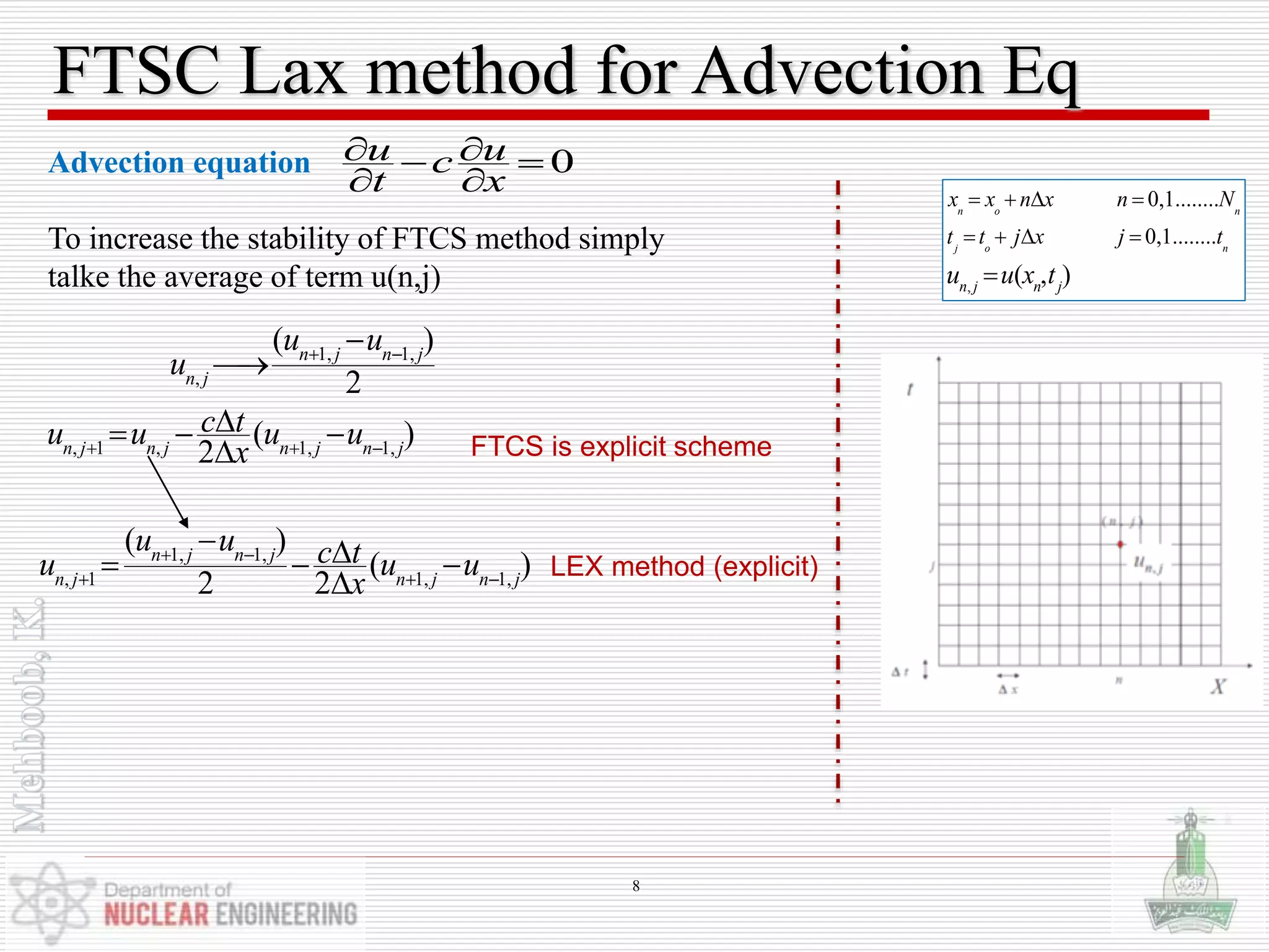
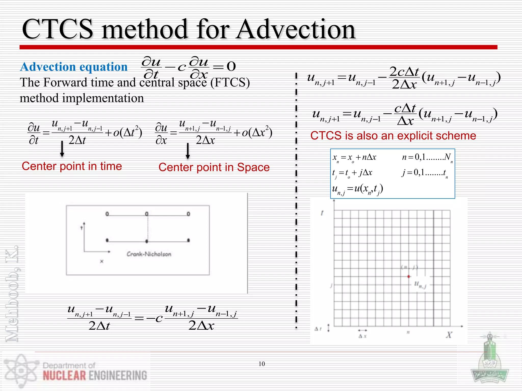
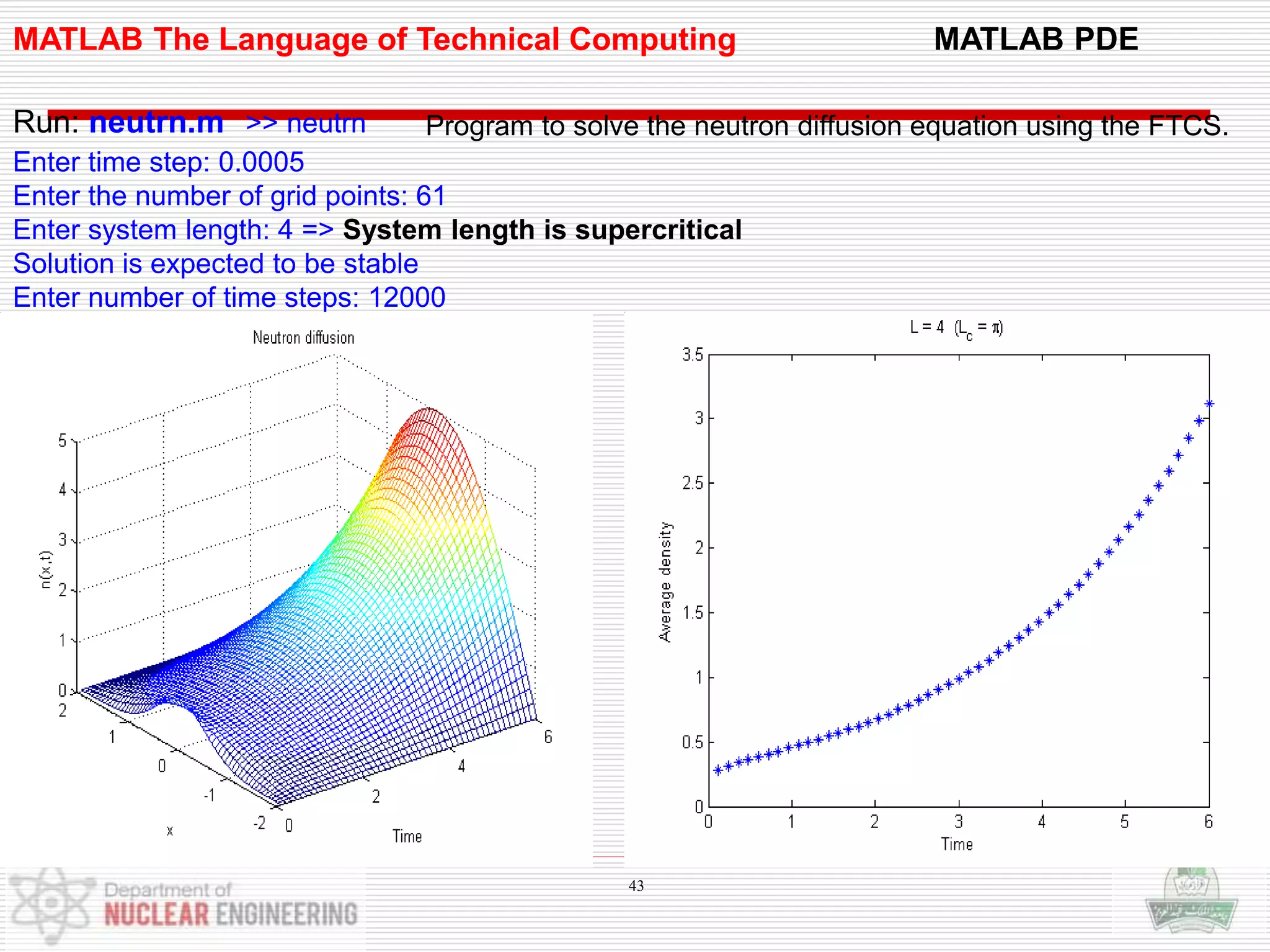
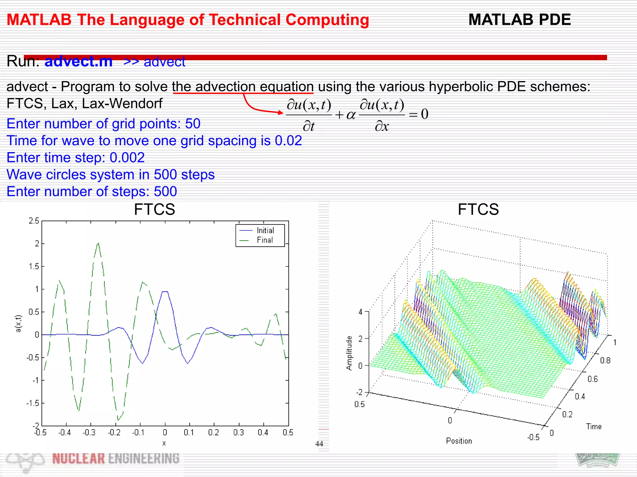
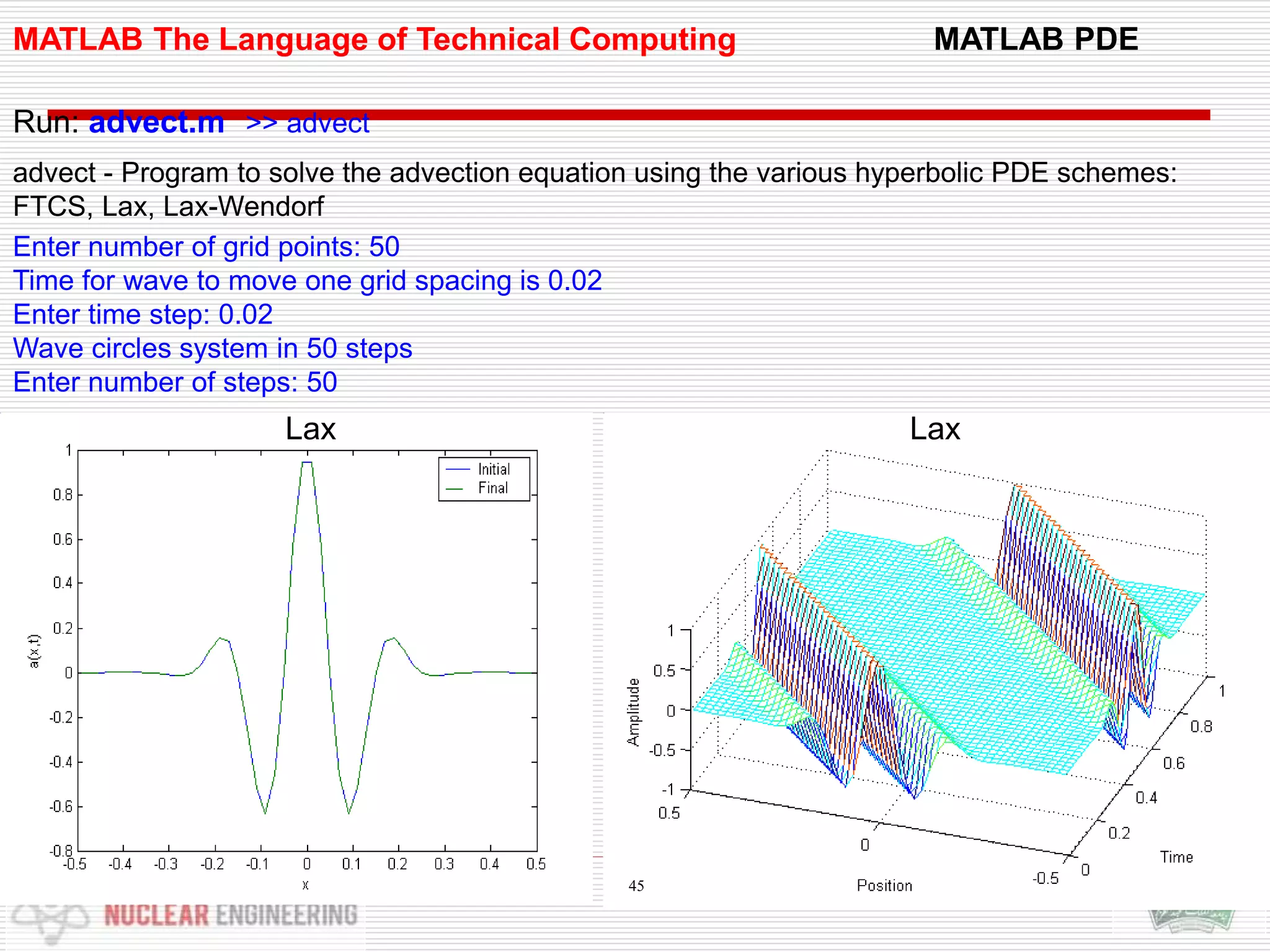
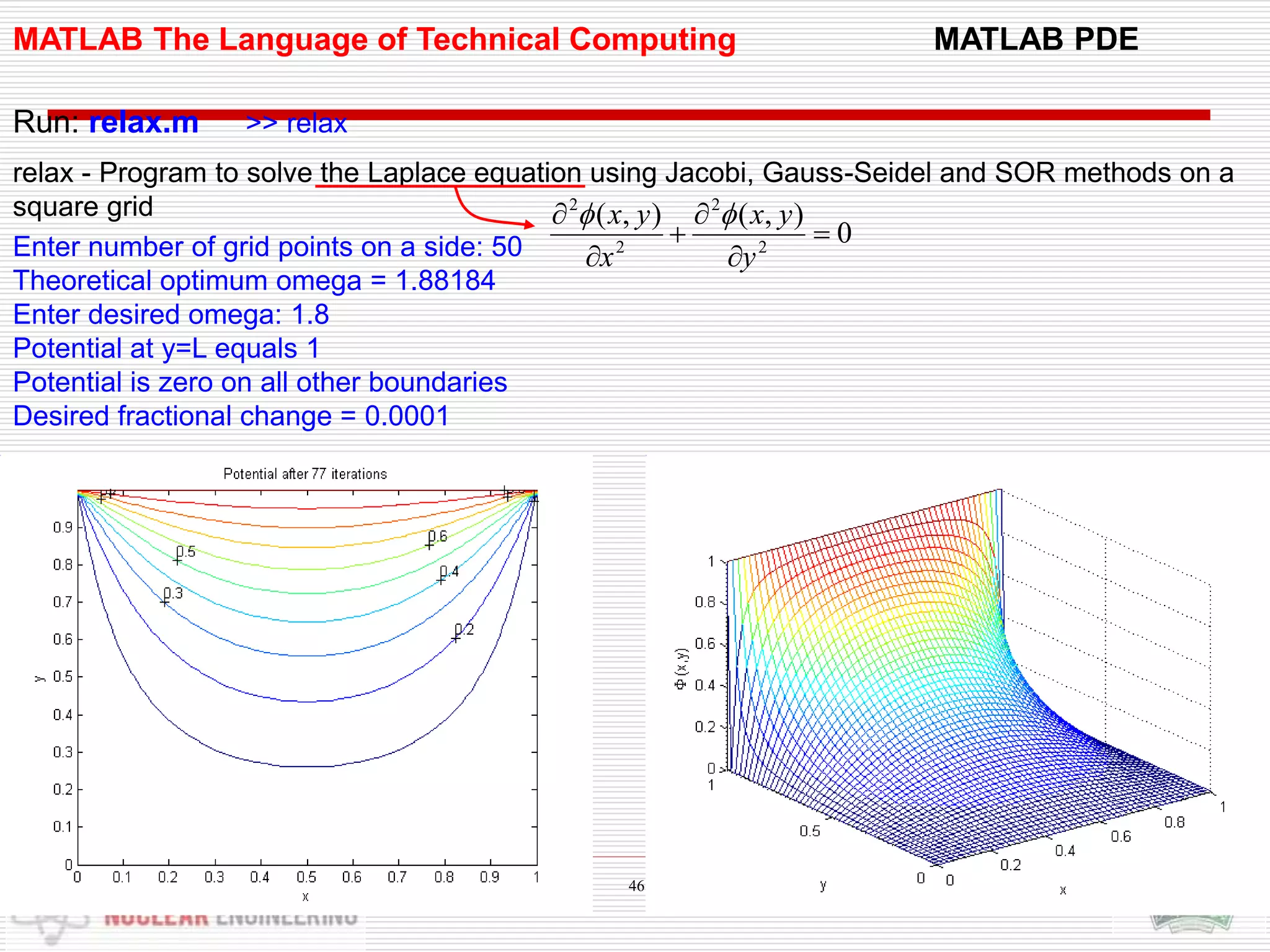
This document discusses various computational methods for solving partial differential equations (PDEs) using MATLAB. It begins by introducing three types of PDEs - elliptic, parabolic, and hyperbolic - and provides examples of each. It then describes explicit methods like the Forward Time Centered Space (FTCS) method, Lax method, and Crank-Nicolson (CTCS) method for solving the advection equation. The document provides MATLAB code implementing these methods for a test case of solving the advection equation modeling a square wave.