The document is lecture notes on computational fluid dynamics (CFD) using the finite volume method. It contains 8 chapters covering basic concepts in fluid dynamics, the finite difference method, the finite volume method, solving CFD problems with ANSYS/CFX software, creating CFD meshes with ICEM software, and applying CFD in engineering. Chapter 5 focuses on the finite volume method and provides examples of applying it to 1D steady state diffusion problems by dividing the domain into control volumes and deriving the discretized equations.
Nguyễn Thanh Nhã 10/16/2018
nhanguyen@hcmut.edu.vn 3
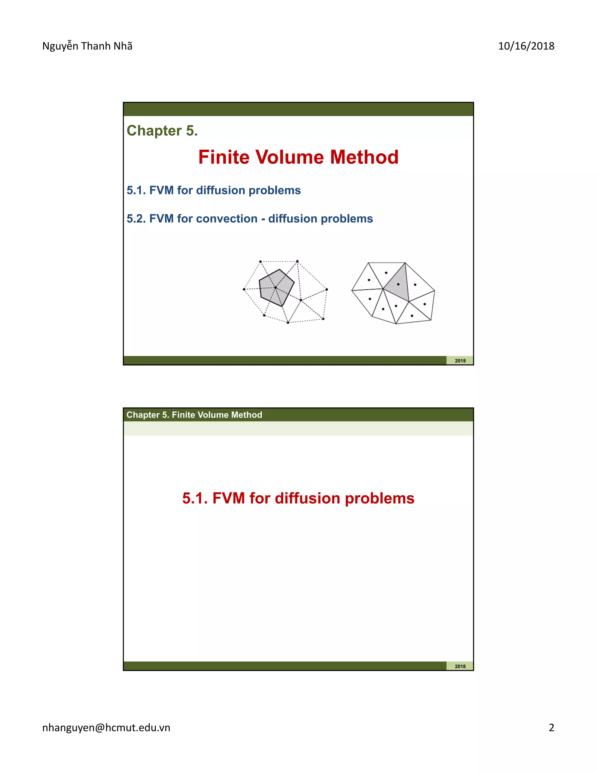
Chapter5. Finite Volume Method
2018
• The numerical method (finite volume or control volume method) based on
is developed for the the simplest transport process:
pure diffusion in the steady state
5.1. FVM for diffusion problems
Introduction
2 2 2
2 2 2
x x x x x x x
x y z x
v v v v p v v v
v v v g
t x y z x x y z
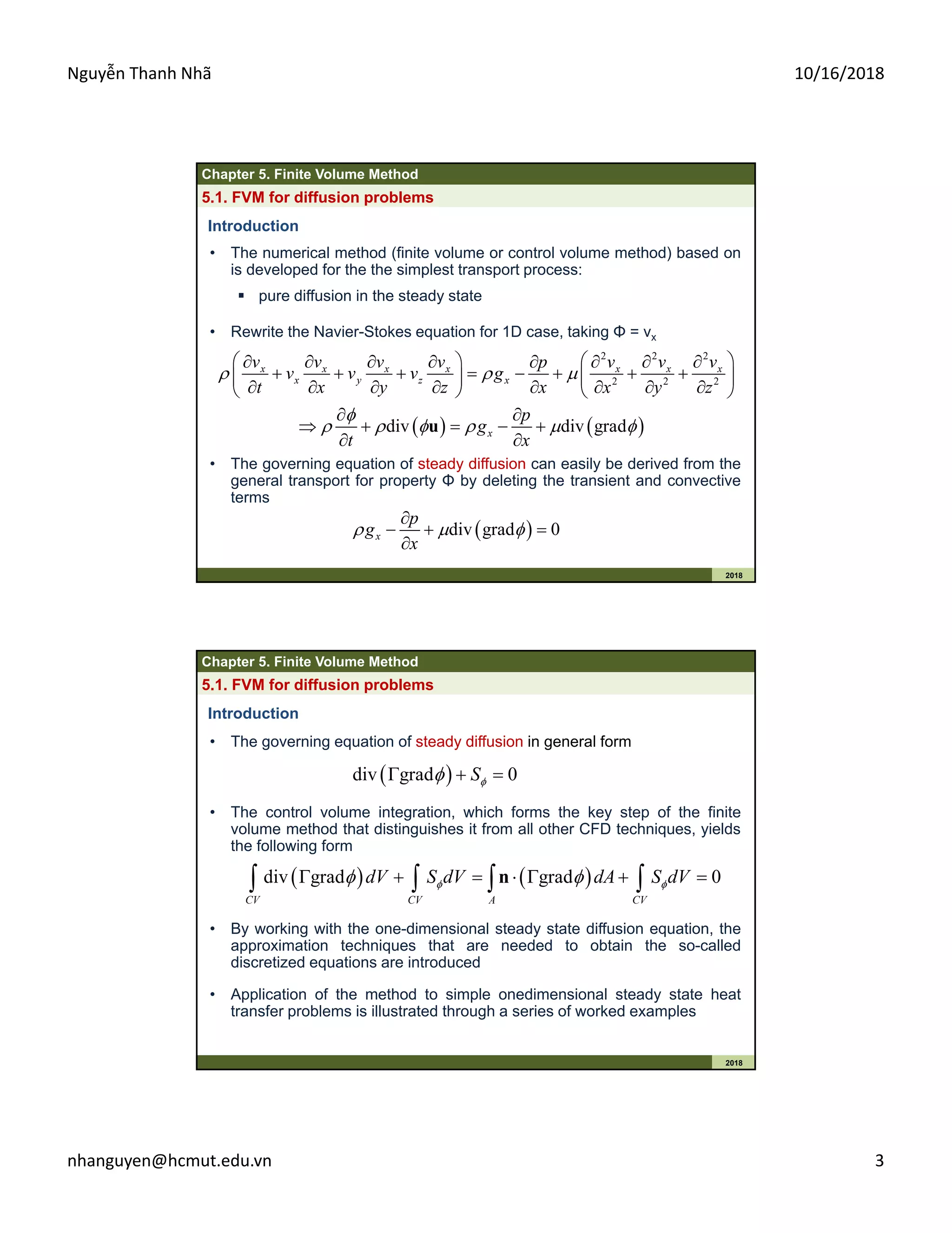
• Rewrite the Navier-Stokes equation for 1D case, taking Φ = vx
div div gradx
p
g
t x
u
• The governing equation of steady diffusion can easily be derived from the
general transport for property Φ by deleting the transient and convective
terms
div grad 0x
p
g
x
Chapter 5. Finite Volume Method
2018
5.1. FVM for diffusion problems
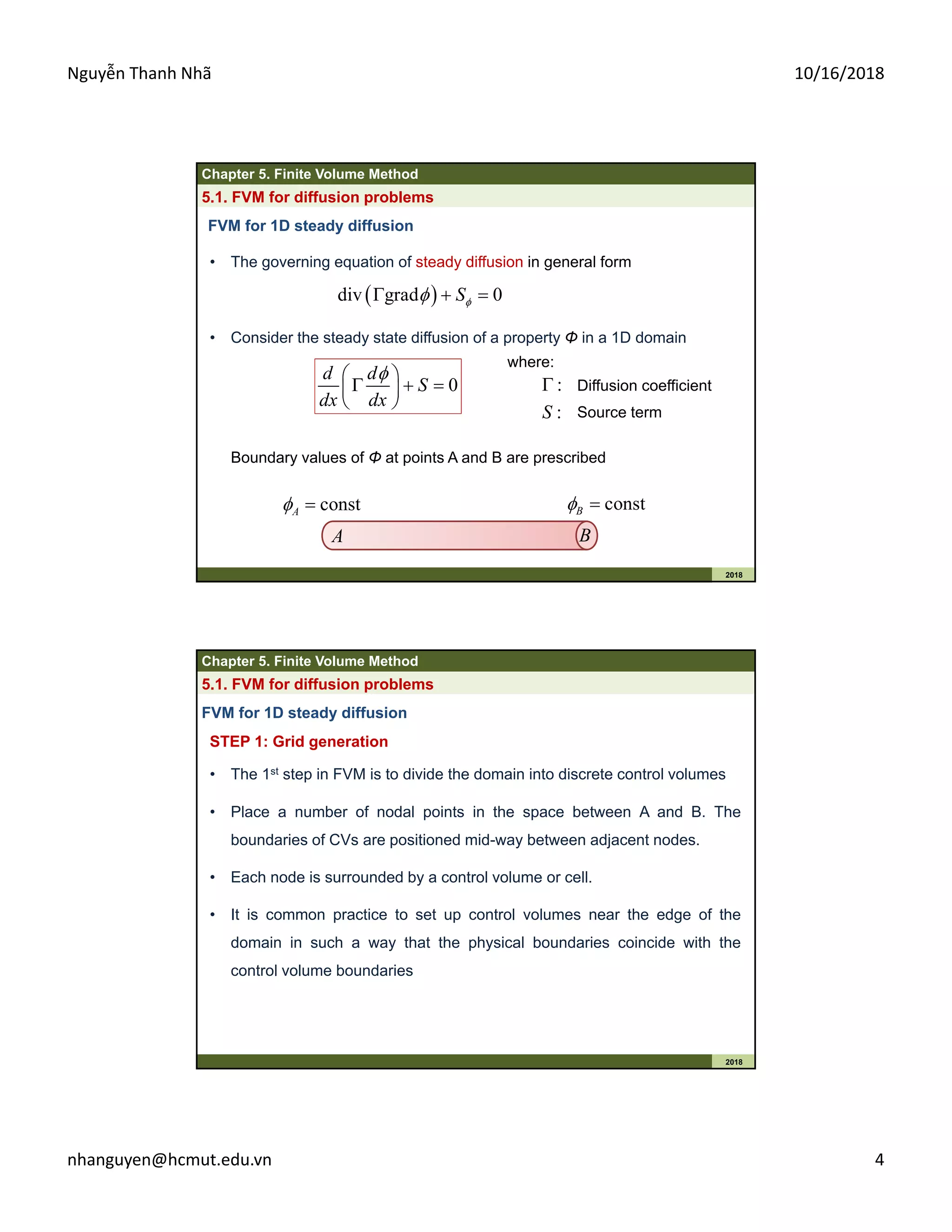
• The governing equation of steady diffusion in general form
Introduction
div grad 0S
• By working with the one-dimensional steady state diffusion equation, the
approximation techniques that are needed to obtain the so-called
discretized equations are introduced
• The control volume integration, which forms the key step of the finite
volume method that distinguishes it from all other CFD techniques, yields
the following form
div grad grad 0
CV CV A CV
dV S dV dA S dV n
• Application of the method to simple onedimensional steady state heat
transfer problems is illustrated through a series of worked examples
4.
Nguyễn Thanh Nhã 10/16/2018
nhanguyen@hcmut.edu.vn 4
Chapter5. Finite Volume Method
2018
5.1. FVM for diffusion problems
• The governing equation of steady diffusion in general form
FVM for 1D steady diffusion
div grad 0S
where:
: Diffusion coefficient
:S Source term
• Consider the steady state diffusion of a property Φ in a 1D domain
0
d d
S
dx dx
Boundary values of Φ at points A and B are prescribed
A B
constA constB
Chapter 5. Finite Volume Method
2018
5.1. FVM for diffusion problems
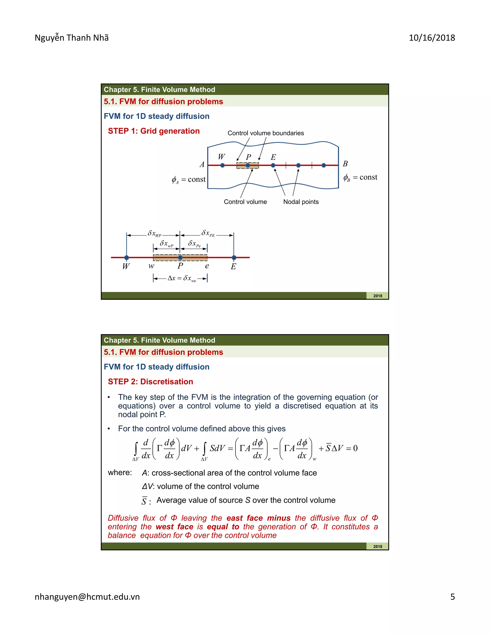
STEP 1: Grid generation
FVM for 1D steady diffusion
• The 1st step in FVM is to divide the domain into discrete control volumes
• Place a number of nodal points in the space between A and B. The
boundaries of CVs are positioned mid-way between adjacent nodes.
• Each node is surrounded by a control volume or cell.
• It is common practice to set up control volumes near the edge of the
domain in such a way that the physical boundaries coincide with the
control volume boundaries
5.
Nguyễn Thanh Nhã 10/16/2018
nhanguyen@hcmut.edu.vn 5
Chapter5. Finite Volume Method
2018
5.1. FVM for diffusion problems
STEP 1: Grid generation
FVM for 1D steady diffusion
A
constB
B
constA
Control volume boundaries
Control volume Nodal points
P EW
PW
wPx
w e
Pex
WPx PEx
wex x
E
Chapter 5. Finite Volume Method
2018
5.1. FVM for diffusion problems
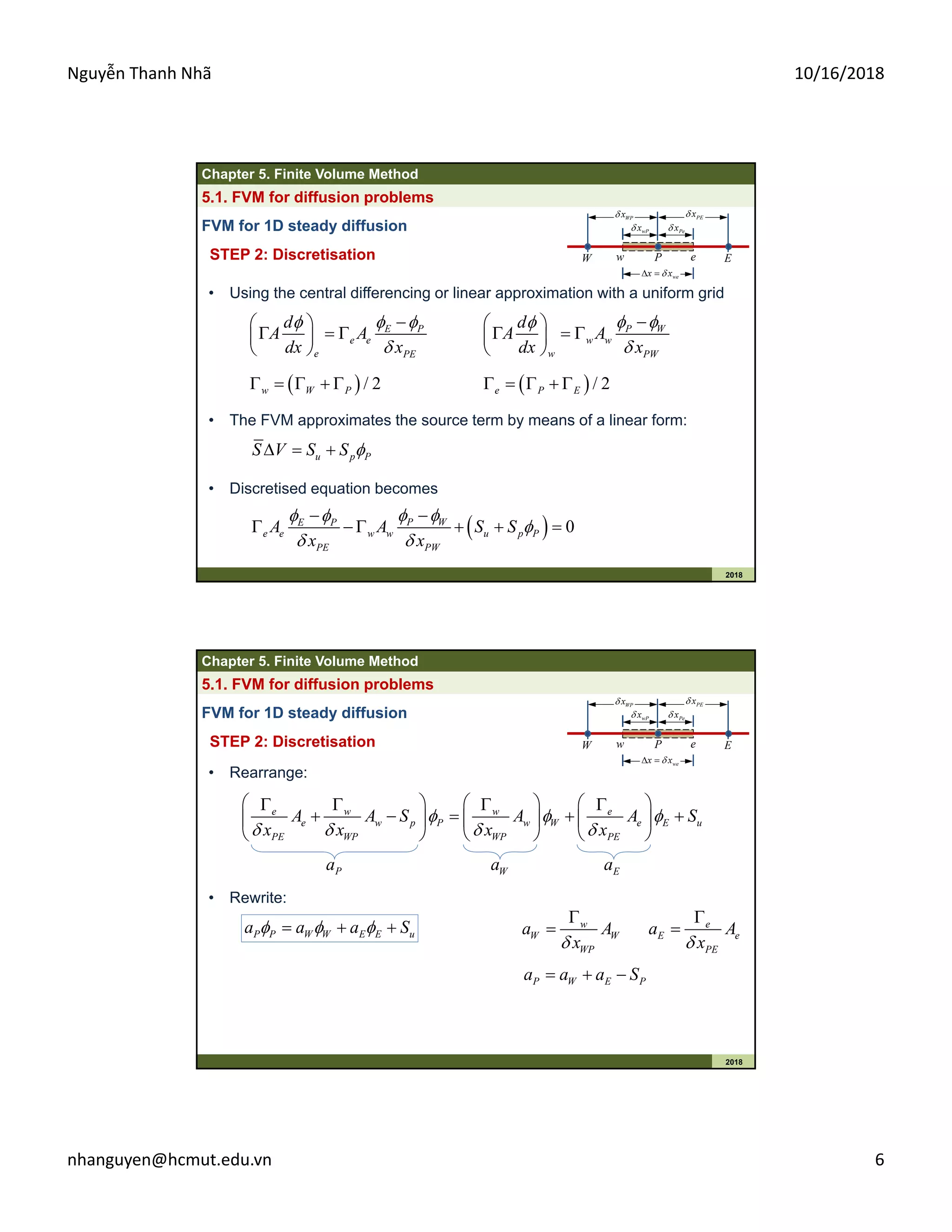
STEP 2: Discretisation
FVM for 1D steady diffusion
• The key step of the FVM is the integration of the governing equation (or
equations) over a control volume to yield a discretised equation at its
nodal point P.
0
e wV V
d d d d
dV SdV A A S V
dx dx dx dx
• For the control volume defined above this gives
where: A: cross-sectional area of the control volume face
ΔV: volume of the control volume
:S Average value of source S over the control volume
Diffusive flux of Φ leaving the east face minus the diffusive flux of Φ
entering the west face is equal to the generation of Φ. It constitutes a
balance equation for Φ over the control volume
6.
Nguyễn Thanh Nhã 10/16/2018
nhanguyen@hcmut.edu.vn 6
Chapter5. Finite Volume Method
2018
5.1. FVM for diffusion problems
STEP 2: Discretisation
FVM for 1D steady diffusion
• Using the central differencing or linear approximation with a uniform grid
E P
e e
e PE
d
A A
dx x
P W
w w
w PW
d
A A
dx x
/ 2w W P / 2e P E
PW
wPx
w e
Pex
WPx PEx
wex x
E
• The FVM approximates the source term by means of a linear form:
u p PS V S S
• Discretised equation becomes
0P WE P
e e w w u p P
PE PW
A A S S
x x
Chapter 5. Finite Volume Method
2018
5.1. FVM for diffusion problems
STEP 2: Discretisation
FVM for 1D steady diffusion
PW
wPx
w e
Pex
WPx PEx
wex x
E
• Rearrange:
e w w e
e w p P w W e E u
PE WP WP PE
A A S A A S
x x x x
Pa Wa Ea
P P W W E E ua a a S
• Rewrite:
P W E Pa a a S
w
W W
WP
a A
x
e
E e
PE
a A
x
7.
Nguyễn Thanh Nhã 10/16/2018
nhanguyen@hcmut.edu.vn 7
Chapter5. Finite Volume Method
2018
5.1. FVM for diffusion problems
STEP 3: Solution of equations
FVM for 1D steady diffusion
• Discretised equations must be set up at each of the nodal points in
order to solve a problem
• For control volumes that are adjacent to the domain boundaries the
general discretised equation is modified to incorporate boundary
conditions.
• The resulting system of linear algebraic equations is then solved to
obtain the distribution of the property Φ at nodal points
Chapter 5. Finite Volume Method
2018
5.1. FVM for diffusion problems
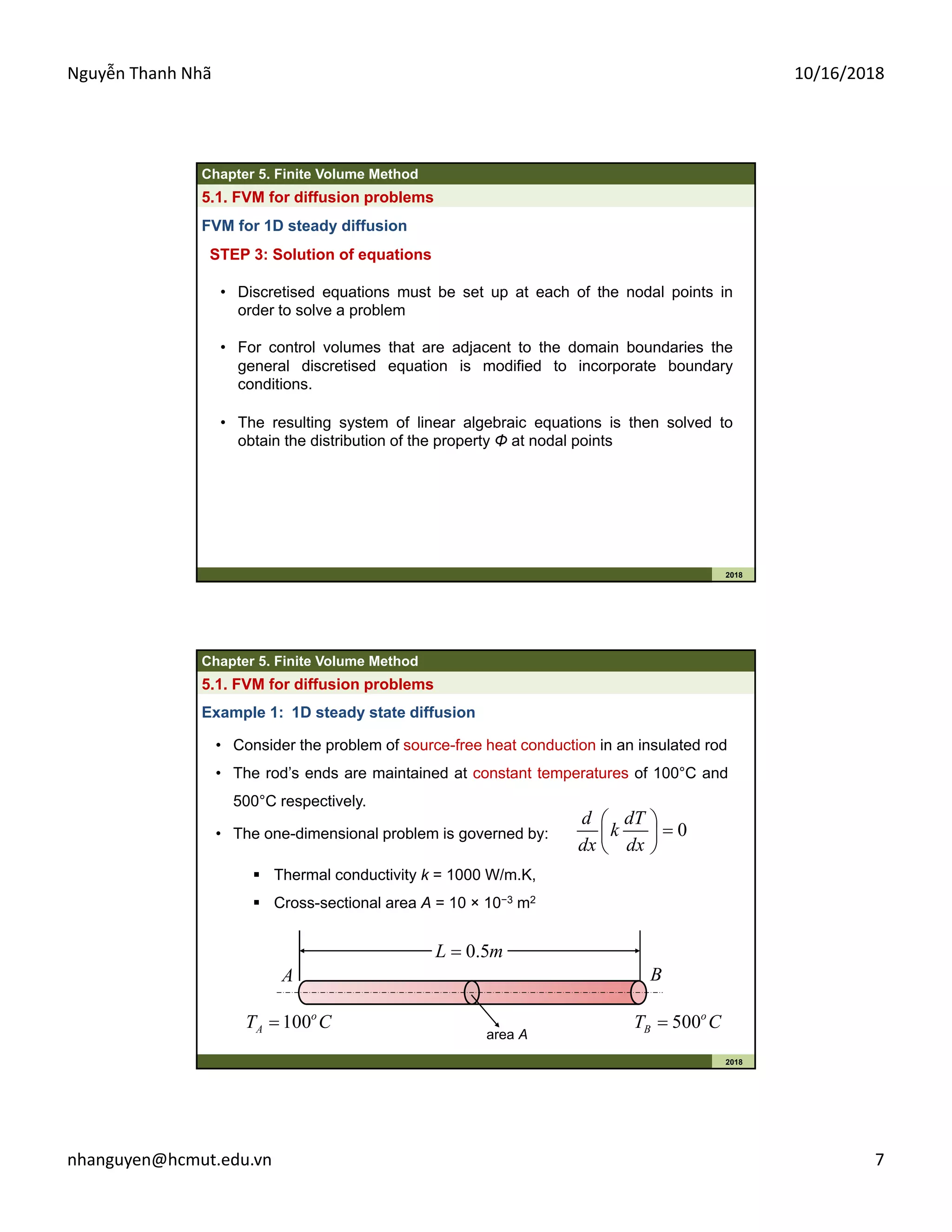
Example 1: 1D steady state diffusion
• Consider the problem of source-free heat conduction in an insulated rod
• The rod’s ends are maintained at constant temperatures of 100°C and
500°C respectively.
• The one-dimensional problem is governed by: 0
d dT
k
dx dx
Thermal conductivity k = 1000 W/m.K,
Cross-sectional area A = 10 × 10−3 m2
0.5L m
area A
A B
100o
AT C 500o
BT C
8.
Nguyễn Thanh Nhã 10/16/2018
nhanguyen@hcmut.edu.vn 8
Chapter5. Finite Volume Method
2018
5.1. FVM for diffusion problems
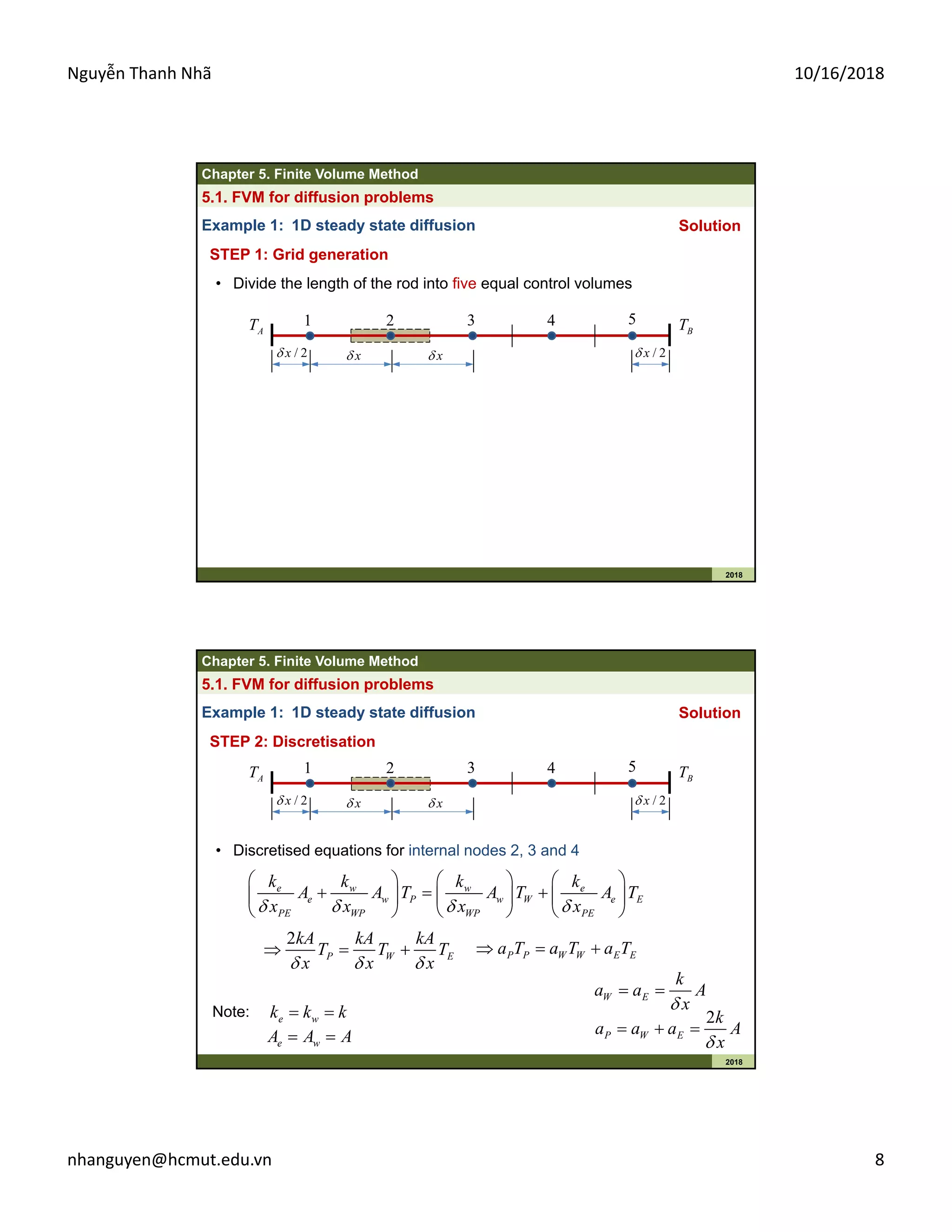
Example 1: 1D steady state diffusion
• Divide the length of the rod into five equal control volumes
Solution
STEP 1: Grid generation
AT 1 2 3 4 5
BT
/ 2x/ 2x x x
Chapter 5. Finite Volume Method
2018
5.1. FVM for diffusion problems
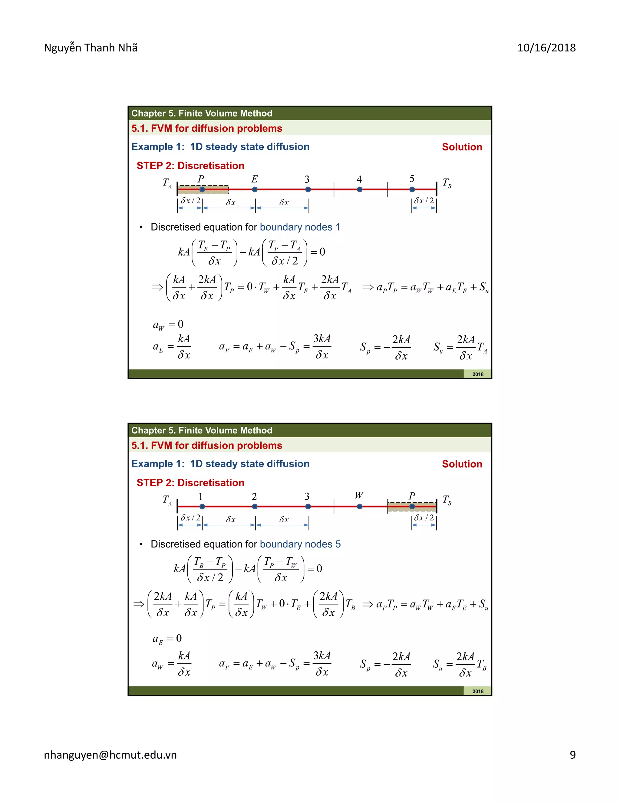
Example 1: 1D steady state diffusion Solution
STEP 2: Discretisation
AT 1 2 3 4 5
BT
/ 2x/ 2x x x
• Discretised equations for internal nodes 2, 3 and 4
e w w e
e w P w W e E
PE WP WP PE
k k k k
A A T A T A T
x x x x
P P W W E Ea T a T a T
2
P W E
k
a a a A
x
W E
k
a a A
x
Note: e wk k k
e wA A A
2
P W E
kA kA kA
T T T
x x x
9.
Nguyễn Thanh Nhã 10/16/2018
nhanguyen@hcmut.edu.vn 9
Chapter5. Finite Volume Method
2018
5.1. FVM for diffusion problems
Example 1: 1D steady state diffusion Solution
STEP 2: Discretisation
AT P E 3 4 5
BT
/ 2x/ 2x x x
• Discretised equation for boundary nodes 1
0
/ 2
E P P AT T T T
kA kA
x x
2 2
0P W E A
kA kA kA kA
T T T T
x x x x
P P W W E E ua T a T a T S
3
P E W p
kA
a a a S
x
0Wa
E
kA
a
x
2
p
kA
S
x
2
u A
kA
S T
x
Chapter 5. Finite Volume Method
2018
5.1. FVM for diffusion problems
Example 1: 1D steady state diffusion Solution
STEP 2: Discretisation
AT 1 2 3 W P
BT
/ 2x/ 2x x x
• Discretised equation for boundary nodes 5
0
/ 2
B P P WT T T T
kA kA
x x
P P W W E E ua T a T a T S
3
P E W p
kA
a a a S
x
0Ea
W
kA
a
x
2
p
kA
S
x
2
u B
kA
S T
x
2 2
0P W E B
kA kA kA kA
T T T T
x x x x
10.
Nguyễn Thanh Nhã 10/16/2018
nhanguyen@hcmut.edu.vn 10
Chapter5. Finite Volume Method
2018
5.1. FVM for diffusion problems
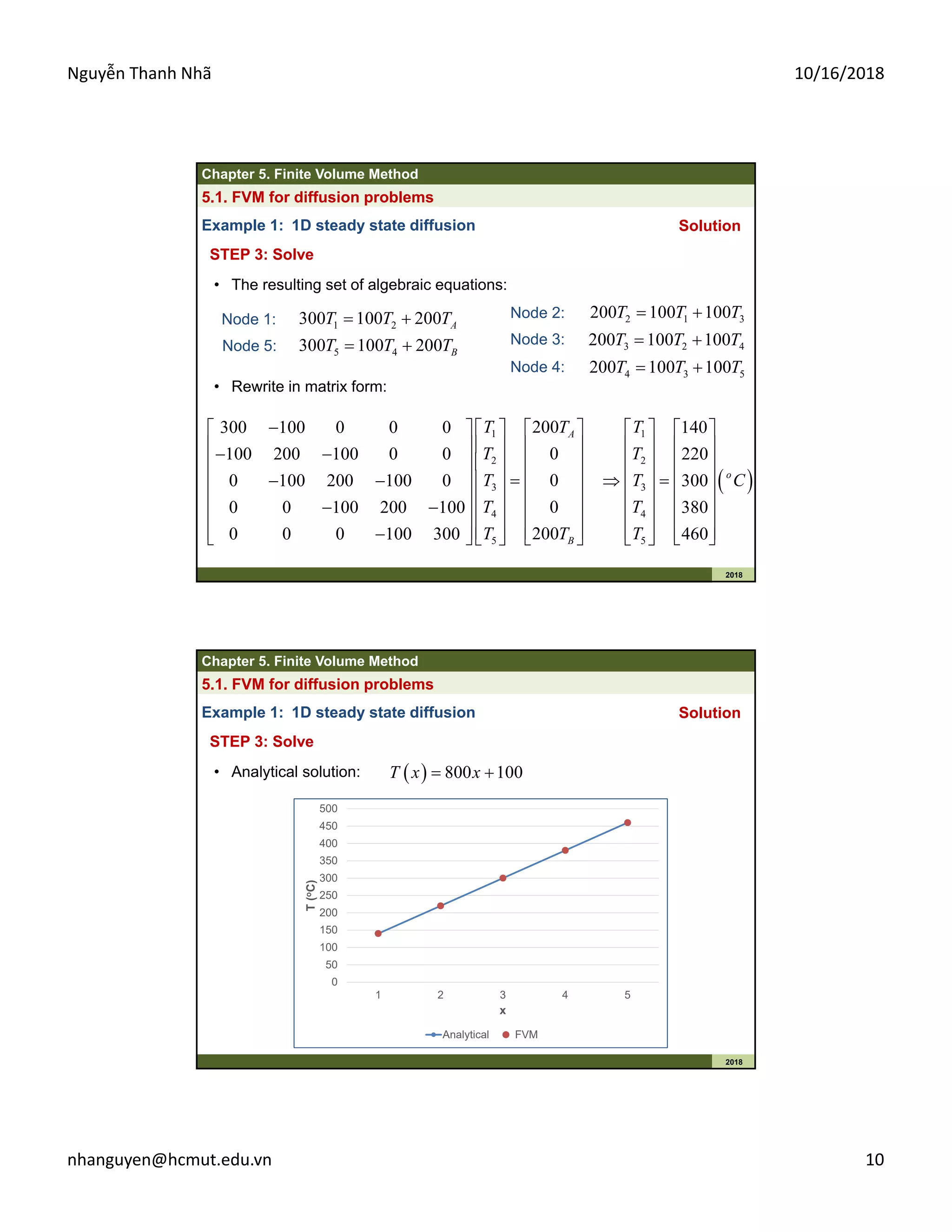
Example 1: 1D steady state diffusion Solution
STEP 3: Solve
• The resulting set of algebraic equations:
1 2300 100 200 AT T T Node 1: 2 1 3200 100 100T T T Node 2:
3 2 4200 100 100T T T Node 3:
4 3 5200 100 100T T T Node 4:
5 4300 100 200 BT T T Node 5:
1
2
3
4
5
200300 100 0 0 0
0100 200 100 0 0
00 100 200 100 0
00 0 100 200 100
2000 0 0 100 300
A
B
T T
T
T
T
T T
1
2
3
4
5
140
220
300
380
460
o
T
T
T C
T
T
• Rewrite in matrix form:
Chapter 5. Finite Volume Method
2018
5.1. FVM for diffusion problems
Example 1: 1D steady state diffusion Solution
STEP 3: Solve
• Analytical solution: 800 100T x x
0
50
100
150
200
250
300
350
400
450
500
1 2 3 4 5
T(oC)
x
Analytical FVM
11.
Nguyễn Thanh Nhã 10/16/2018
nhanguyen@hcmut.edu.vn 11
Chapter5. Finite Volume Method
2018
5.1. FVM for diffusion problems
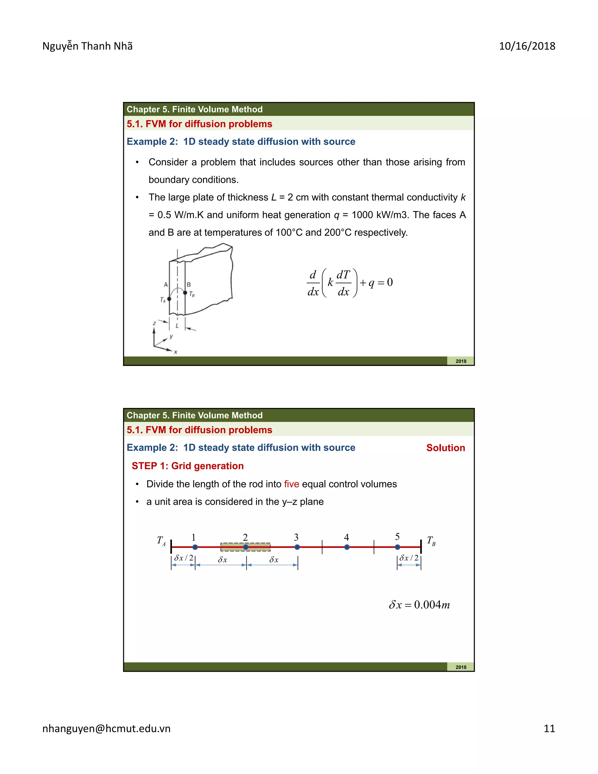
Example 2: 1D steady state diffusion with source
• Consider a problem that includes sources other than those arising from
boundary conditions.
• The large plate of thickness L = 2 cm with constant thermal conductivity k
= 0.5 W/m.K and uniform heat generation q = 1000 kW/m3. The faces A
and B are at temperatures of 100°C and 200°C respectively.
0
d dT
k q
dx dx
Chapter 5. Finite Volume Method
2018
5.1. FVM for diffusion problems
Example 2: 1D steady state diffusion with source
• Divide the length of the rod into five equal control volumes
• a unit area is considered in the y–z plane
Solution
STEP 1: Grid generation
AT 1 2 3 4 5
BT
/ 2x/ 2x x x
0.004x m
12.
Nguyễn Thanh Nhã 10/16/2018
nhanguyen@hcmut.edu.vn 12
Chapter5. Finite Volume Method
2018
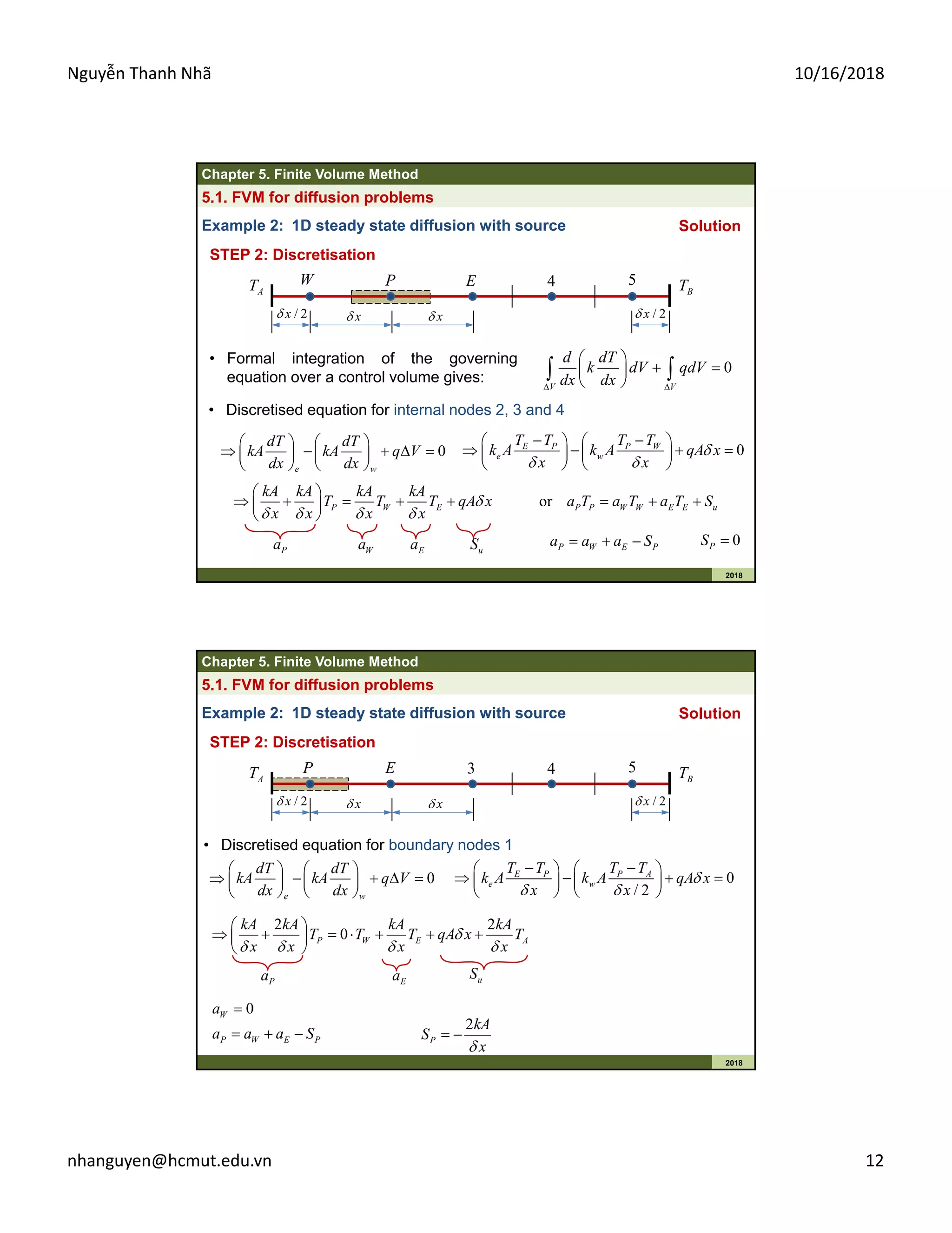
5.1. FVM for diffusion problems
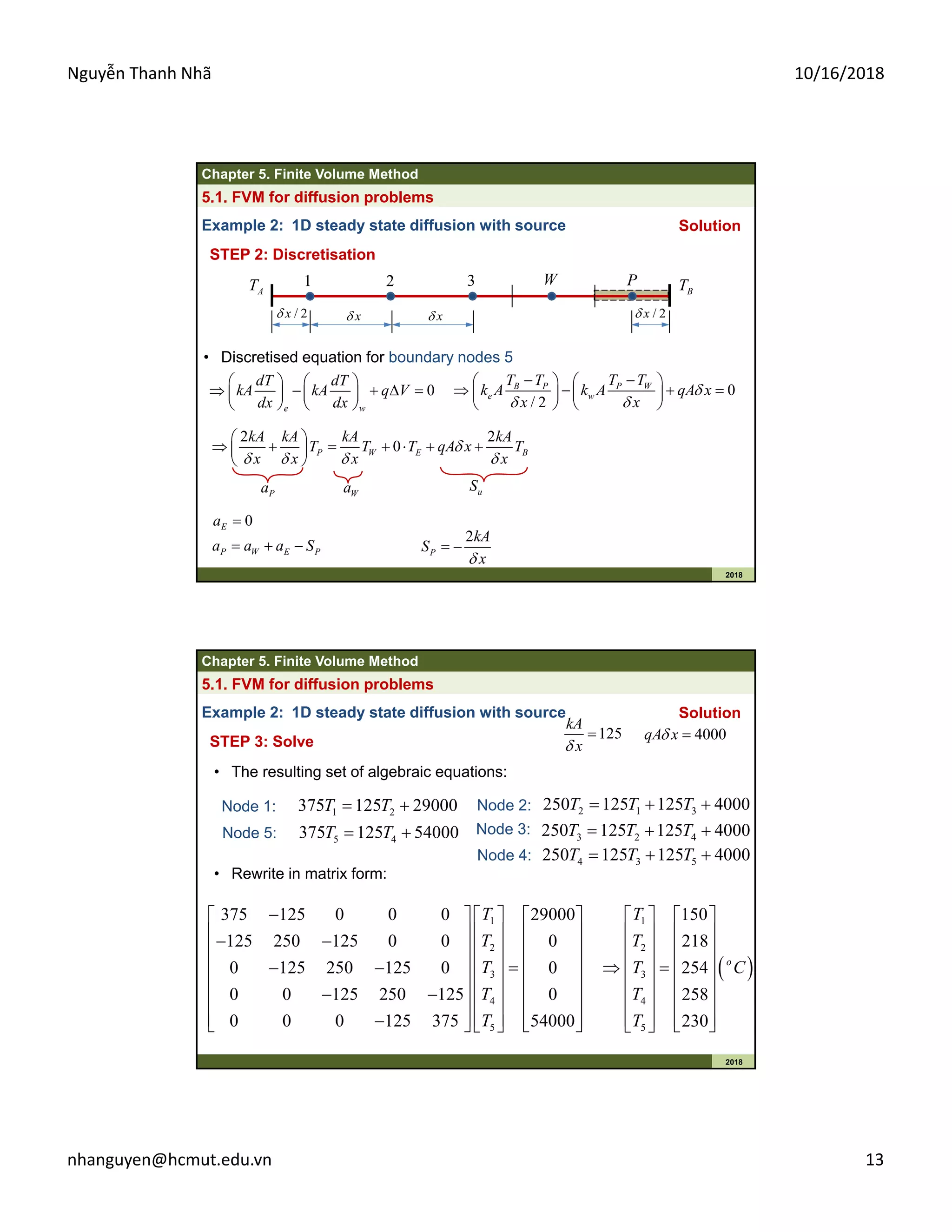
Example 2: 1D steady state diffusion with source Solution
STEP 2: Discretisation
AT W P E 4 5
BT
/ 2x/ 2x x x
• Formal integration of the governing
equation over a control volume gives:
0
V V
d dT
k dV qdV
dx dx
0
e w
dT dT
kA kA q V
dx dx
0P WE P
e w
T TT T
k A k A qA x
x x
P W E
kA kA kA kA
T T T qA x
x x x x
or P P W W E E ua T a T a T S
Pa Wa Ea uS 0PS
• Discretised equation for internal nodes 2, 3 and 4
P W E Pa a a S
Chapter 5. Finite Volume Method
2018
5.1. FVM for diffusion problems
Example 2: 1D steady state diffusion with source Solution
STEP 2: Discretisation
AT P E 3 4 5
BT
/ 2x/ 2x x x
• Discretised equation for boundary nodes 1
0
e w
dT dT
kA kA q V
dx dx
0
/ 2
E P P A
e w
T T T T
k A k A qA x
x x
2 2
0P W E A
kA kA kA kA
T T T qA x T
x x x x
Pa Ea uS
0Wa
P W E Pa a a S
2
P
kA
S
x
13.
Nguyễn Thanh Nhã 10/16/2018
nhanguyen@hcmut.edu.vn 13
Chapter5. Finite Volume Method
2018
5.1. FVM for diffusion problems
Example 2: 1D steady state diffusion with source Solution
STEP 2: Discretisation
AT 1 2 3 W P
BT
/ 2x/ 2x x x
• Discretised equation for boundary nodes 5
0
e w
dT dT
kA kA q V
dx dx
0
/ 2
P WB P
e w
T TT T
k A k A qA x
x x
2 2
0P W E B
kA kA kA kA
T T T qA x T
x x x x
Pa Wa uS
0Ea
P W E Pa a a S
2
P
kA
S
x
Chapter 5. Finite Volume Method
2018
5.1. FVM for diffusion problems
Solution
STEP 3: Solve
• The resulting set of algebraic equations:
1 2375 125 29000T T Node 1: 2 1 3250 125 125 4000T T T Node 2:
3 2 4250 125 125 4000T T T Node 3:
4 3 5250 125 125 4000T T T Node 4:
5 4375 125 54000T T Node 5:
1
2
3
4
5
375 125 0 0 0 29000
125 250 125 0 0 0
0 125 250 125 0 0
0 0 125 250 125 0
0 0 0 125 375 54000
T
T
T
T
T
1
2
3
4
5
150
218
254
258
230
o
T
T
T C
T
T
• Rewrite in matrix form:
125
kA
x
4000qA x
Example 2: 1D steady state diffusion with source
14.
Nguyễn Thanh Nhã 10/16/2018
nhanguyen@hcmut.edu.vn 14
Chapter5. Finite Volume Method
2018
5.1. FVM for diffusion problems
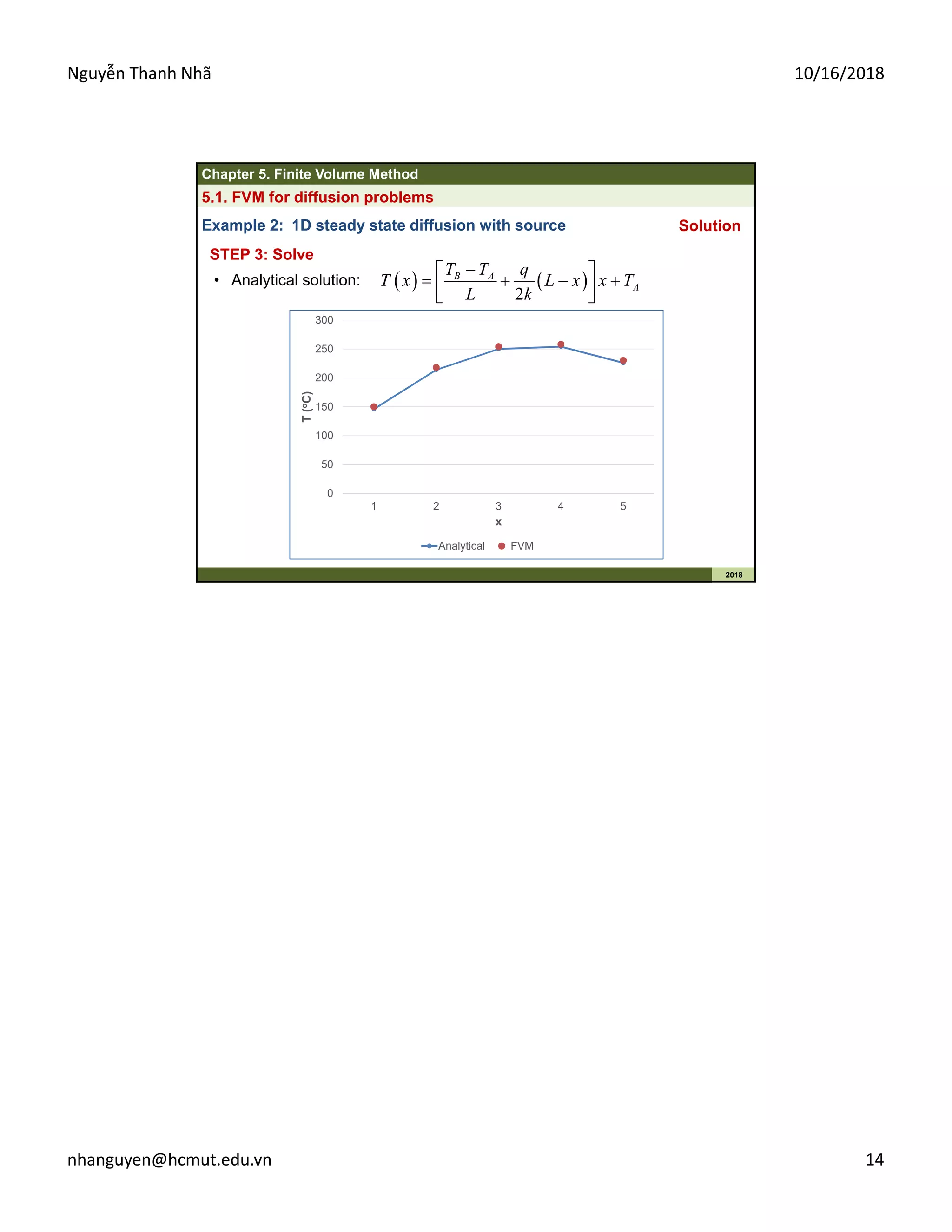
Solution
STEP 3: Solve
• Analytical solution:
2
B A
A
T T q
T x L x x T
L k
0
50
100
150
200
250
300
1 2 3 4 5
T(oC)
x
Analytical FVM
Example 2: 1D steady state diffusion with source


![ANPARA THERMAL POWER STATION[1] sangam.pdf](https://cdn.slidesharecdn.com/ss_thumbnails/anparathermalpowerstation1sangam-251121115219-9261cde4-thumbnail.jpg?width=640&height=640&fit=bounds)


