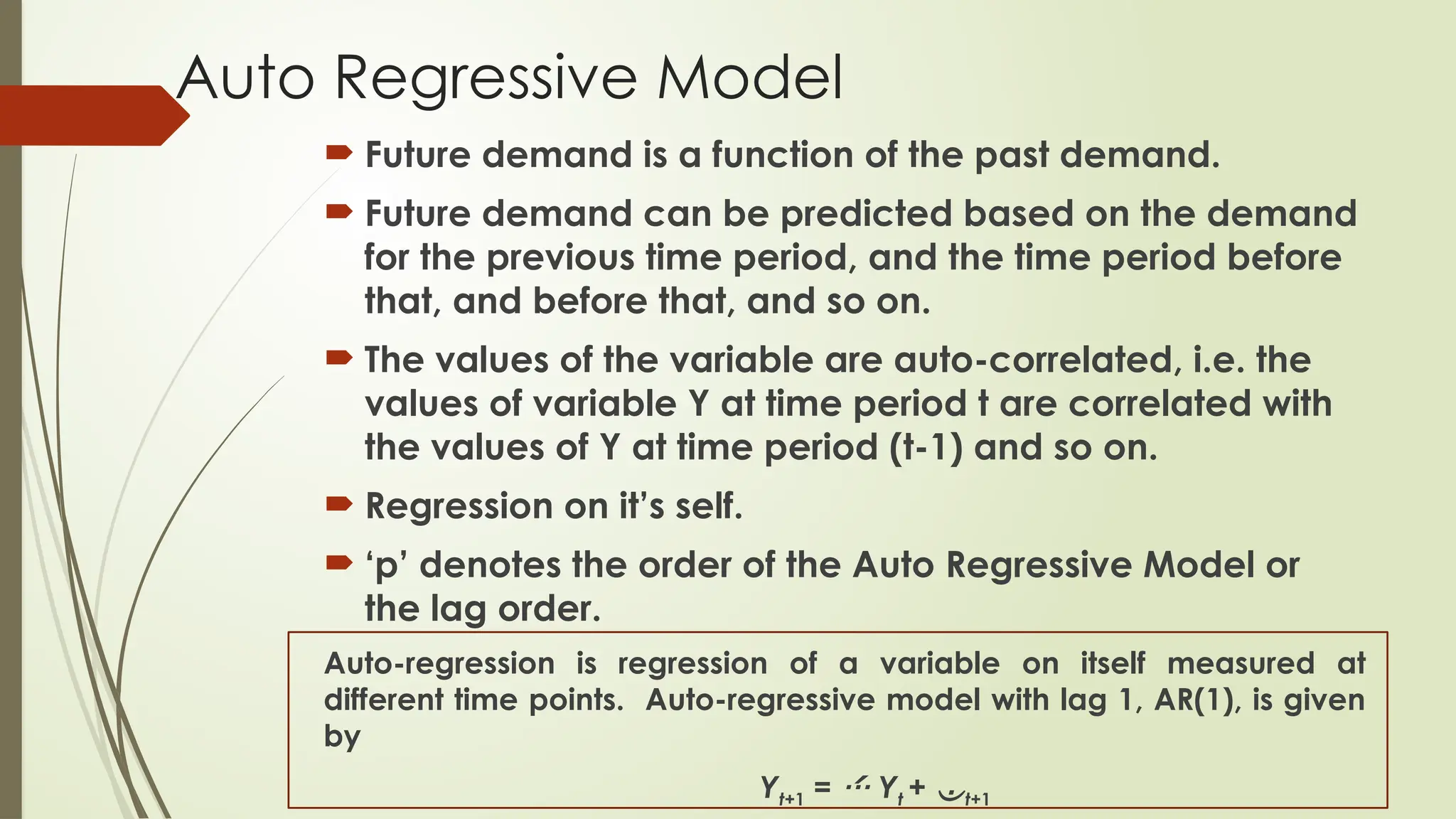
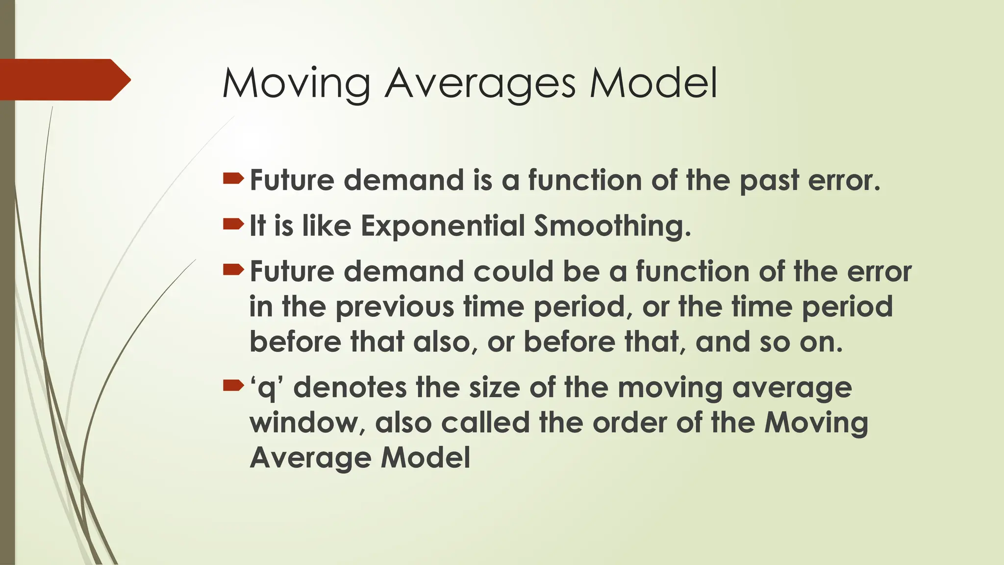
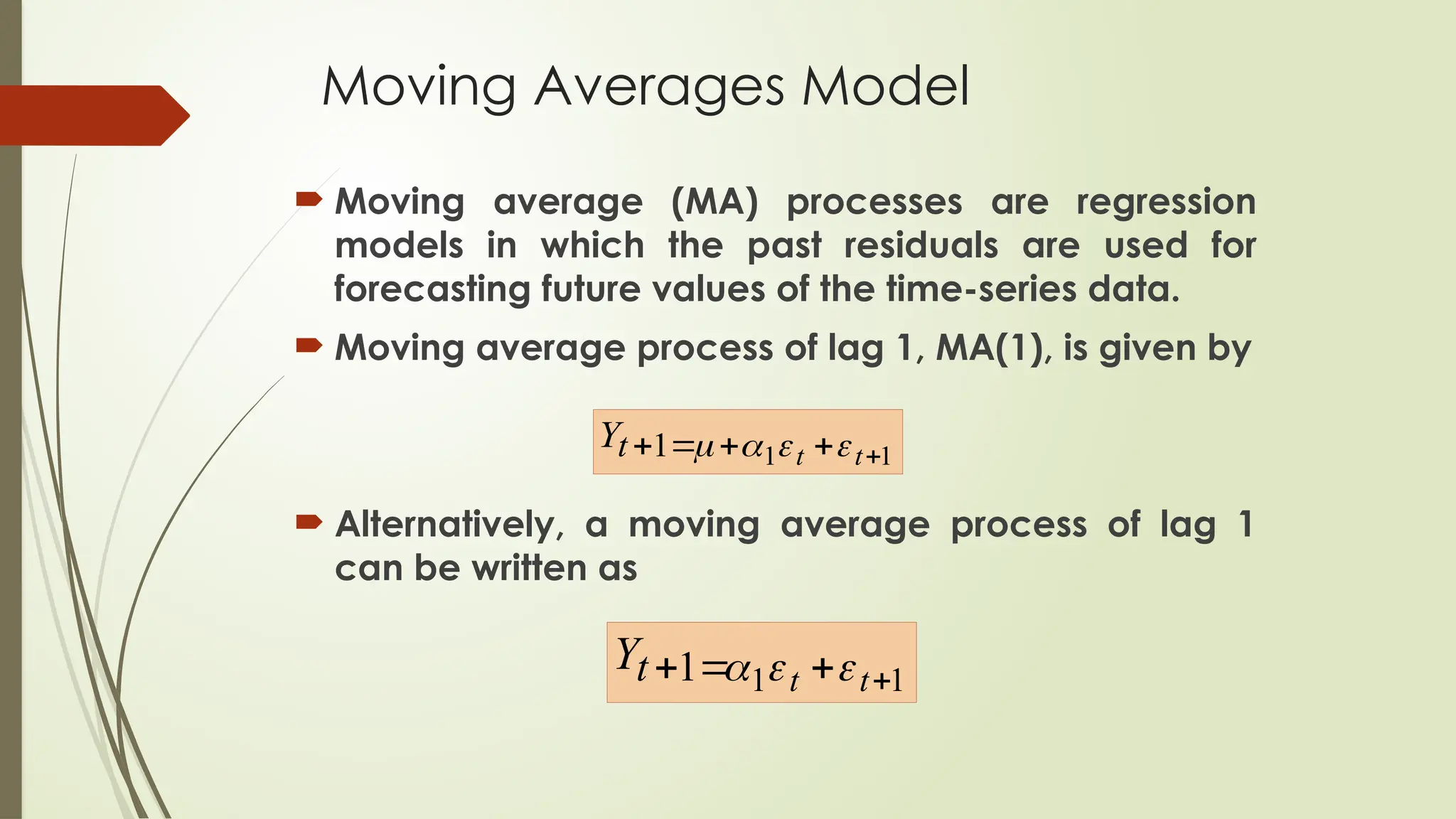
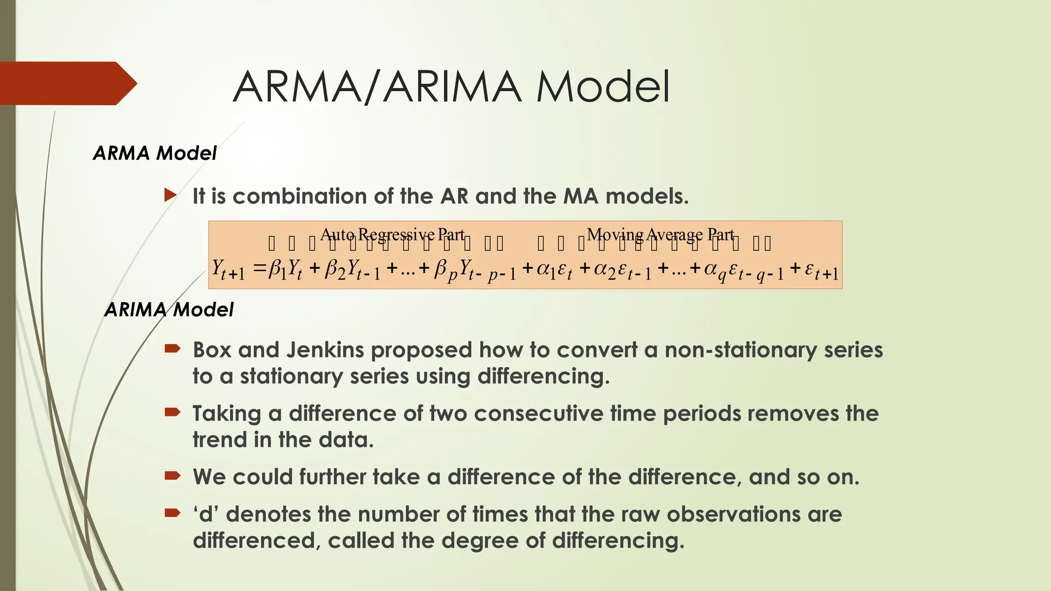
 Box Jenkins Method of
Forecasting
Or
 ARIMA MODEL
Time Series
Non Stationary
No Trend Trend
Stationary
Seasonal Only Trend
Overview
Stationary Series
It has a constant mean
It has a constant variance
No Seasonality
1 4 7 10 13 16 19 22 25 28 31 34 37 40 43 46 49 52 55 58 61 64 67 70 73 76 79 82 85 88 91 94 97 100 103 106 109 112 115
0
20
40
60
80
100
120
140
160
180
Stationary Series
1 4 7 10 13 16 19 22 25 28 31 34 37 40 43 46 49 52 55 58 61 64 67 70 73 76 79 82 85 88 91 94 97 100 103 106 109 112 115
0
5
10
15
20
25
Non-Stationary Series
Testing for Stationary Data
Visual Tests
Global vs Local
Augmented Dicky Fuller or ADF test
White Noise
It is a Time Series with:
Mean = 0
Standard deviation is constant with time
Lags are not auto correlated.
Testing for White Noise
Visual Tests
Global vs Local
Check ACF
Auto Correlation
The measurement of some value at a time
period is dependent on the measurement
of that value at the previous time period
and the period before that and so on.
Partial Auto Correlation
It is the direct component of the Auto
Correlation.
It is the direct effect of the variable at some
previous time period on the value of the variable
today.
It helps us find the strength of the direct
correlation between Y(t-1) and Y(t+1) after removing
the indirect effects
ACF/PACF
 ACF (Autocorrelation Function) is a plot that summarizes
the correlation of an observation with lag values.
 The X axis shows the lag and the Y axis shows the
correlation coefficient between -1 and 1 for negative
and positive correlation.
 PACF (Partial Autocorrelation Function) is the plot used to
summarize the correlation of an observation with lag
values that is not accounted for by other lagged
observations at shorter time periods. It is the plot of the
direct effect.
Auto Regressive Model
 Future demand is a function of the past demand.
 Future demand can be predicted based on the demand
for the previous time period, and the time period before
that, and before that, and so on.
 The values of the variable are auto-correlated, i.e. the
values of variable Y at time period t are correlated with
the values of Y at time period (t-1) and so on.
 Regression on it’s self.
 ‘p’ denotes the order of the Auto Regressive Model or
the lag order.
Auto-regression is regression of a variable on itself measured at
different time points. Auto-regressive model with lag 1, AR(1), is given
by
Yt+1 =  Yt + t+1
Moving Averages Model
Future demand is a function of the past error.
It is like Exponential Smoothing.
Future demand could be a function of the error
in the previous time period, or the time period
before that also, or before that, and so on.
‘q’ denotes the size of the moving average
window, also called the order of the Moving
Average Model
Moving Averages Model
 Moving average (MA) processes are regression
models in which the past residuals are used for
forecasting future values of the time-series data.
 Moving average process of lag 1, MA(1), is given by
 Alternatively, a moving average process of lag 1
can be written as
1
1
1 



 t
t
t
Y 



1
1
1 


 t
t
t
Y 


ARMA/ARIMA Model
 Box and Jenkins proposed how to convert a non-stationary series
to a stationary series using differencing.
 Taking a difference of two consecutive time periods removes the
trend in the data.
 We could further take a difference of the difference, and so on.
 ‘d’ denotes the number of times that the raw observations are
differenced, called the degree of differencing.
 It is combination of the AR and the MA models.
ARMA Model
ARIMA Model
1
Part
Average
Moving
1
1
2
1
Part
Regressive
Auto
1
1
2
1
1 ...
... 






 







 t
q
t
q
t
t
p
t
p
t
t
t Y
Y
Y
Y 













 




 





 




 

Model Building
Identification
Estimation
Diagnostic Checking
Forecasting
ARIMA(p, d, q) Model Building
Identification
Check whether the time series is stationary.
If not, check how many differences are required
to make it stationary, i.e. what is the value of ‘d’.
Identify the parameters of the ARMA model for
the data, i.e. what are the values of ‘p’ and ‘q’.
Some Guidelines
 The model is AR if the ACF trails off after a lag and has a
hard cut-off in the PACF after a lag. This is taken as the
value of ‘p’.
 The model is MA if the PACF trails off after a lag and has
a hard cut-off in the ACF after a lag. This lag value is
taken as the ‘q’ value.
 The model is a mix of both AR and MA if both ACF and
PACF trail off.
 In the ACF plot, if there is a positive correlation at lag 1,
use the AR model. If there is a negative correlation at lag
1, use the MA model.
Diagnostic Checking
Check the model for robustness and optimality.
Check for:
Overfitting - Make sure the model is not more
complex than necessary
Residual Errors –
A. Should resemble White Noise
B. Create ACF and PACF plots of the residual
error time series to make sure
there is no auto-correlation
Requirements for a Good Fit
Normalized BIC should be minimum
Ljung Box test should not be significant
H0: Model does not show lack of fit.
H1: Model shows lack of fit.
All coefficients should be significant
ACF and PACF plots of the residual should be
within limits.
White
Noise
Stationary - Visual Test
Trend
ADF
ACF
Idly No
Mean and Variance not
constant, Appears Not
Stationary -7.15
Gradual decrease and then
increase and sharp cutoff
Dosa No
Not Stationary - Variance not
constant -5.86
Dies down extremely slowly
So Not Stationary
Chutney No Appears Stationary -7.3Cuts off sharply So Stationary
Sambhar No Appears Stationary -7.49Cuts off sharply So Stationary
Continental
B/F No Appears Stationary -6.16Cuts off sharply So Stationary
North Indian
B/F No May not be Stationary -7.3
Cuts off sharply, so possibly
Stationary
Omellette No
Not Stationary - Mean and
Variance not constant -3.85
Dies down extremely slowly
So Not Stationary
Idly
Model
R
Square
RMSE MAPE
Normalised
BIC
AIC BIC
LB
Test
Model
Parameters
Significance
Residual
ACF and
PACF
Exponential
Smoothing
0.261 0.24 6.12 7.81 3.67 739 742 Y Y Y
(1,0,0) 0.21 6.29 8.53 3.76 749 755 Y Y Y
(1,1,0) 0.06 6.66 8.05 3.88 N N Y
(0,0,1) 0.15 6.53 9.28 3.84 759 764 N N Y
(0,1,1) 0.14 6.35 7.75 3.77 741 747 Y Y Y
Chutney
Model
R
Square
RMSEMAPE
Normalised
BIC
AIC BIC
LB
Test
Model
Parameters
Significance
Residual
ACF and
PACF
(1,0,0) 0.2 10.0 6.0 4.7 856 861 Y Y Y
(1,1,0) 0.1 10.9 6.6 4.9 870 875 Y N Y
(0,0,1) 0.1 10.2 5.9 4.7 861 867 Y N Y
Exponential
Smoothing
0.39 0.1 10.3 6.2 4.7 858 860 Y Y Y
Omelette
Model
R
Square
RMSE MAPE
Normalised
BIC
AIC BIC
LB
Test
Model
Parameters
Significance
Residual
ACF and
PACF
Exponential
Smoothing
0.618 0.572 3.44 20.59 2.51 608 610 Y Y Y
(1,0,0) 0.584 3.41 21.83 2.53 611 616 Y Y Y
(0,0,1) 0.388 30.09 655 660 N N Y
(1,1,0) 0.525 3.66 21.62 2.68 613 618 Y Y Y
(1,1,1) 0.621 3.33 21.48 2.55 608 616 Y Y Y
Dosa
Model
R
Square
RMSE MAPE Normalised BIC AIC BIC
LB
Test
Model
Parameters
Significance
Residu
ACF a
PAC
Exponential
Smoothing
0.419 0.26 9.81 23.70 4.61 846 849 Y Y Y
(0,0,1) 0.20 10.21 27.24 4.73 863 868 N N Y
(1,0,0) 0.29 9.61 23.79 4.60 849 855 Y N Y
(1,1,0) 0.20 10.29 23.87 4.74 857 863 Y N Y
(1,1,1) 0.28 9.80 23.72 4.69 847 855 Y Y Y
(0,1,1) 0.26 9.89 23.48 4.67 848 854 Y Y Y
Continental B/F
Model
R
Square
RMSE MAPE
Normalised
BIC
AIC BIC LB Test
Model
Parameters
Significance
Residual
ACF and
PACF
(0,0,1) 0.28 4.93 9.15 3.27 693 698 Y Y Y
(1,0,0) 0.28 4.95 8.93 3.28 693 699 Y Y Y
(1,1,0) 0.06 5.44 9.08 3.47 712 718 Y N N
(0,1,1) 0.07 5.43 9.13 3.47 711 717 N N Y
Thank You

ARIMA model predicts futture values based on past values

  • 1.
     Box JenkinsMethod of Forecasting Or  ARIMA MODEL
  • 2.
    Time Series Non Stationary NoTrend Trend Stationary Seasonal Only Trend Overview
  • 3.
    Stationary Series It hasa constant mean It has a constant variance No Seasonality
  • 4.
    1 4 710 13 16 19 22 25 28 31 34 37 40 43 46 49 52 55 58 61 64 67 70 73 76 79 82 85 88 91 94 97 100 103 106 109 112 115 0 20 40 60 80 100 120 140 160 180 Stationary Series 1 4 7 10 13 16 19 22 25 28 31 34 37 40 43 46 49 52 55 58 61 64 67 70 73 76 79 82 85 88 91 94 97 100 103 106 109 112 115 0 5 10 15 20 25 Non-Stationary Series
  • 5.
    Testing for StationaryData Visual Tests Global vs Local Augmented Dicky Fuller or ADF test
  • 6.
    White Noise It isa Time Series with: Mean = 0 Standard deviation is constant with time Lags are not auto correlated.
  • 7.
    Testing for WhiteNoise Visual Tests Global vs Local Check ACF
  • 8.
    Auto Correlation The measurementof some value at a time period is dependent on the measurement of that value at the previous time period and the period before that and so on.
  • 9.
    Partial Auto Correlation Itis the direct component of the Auto Correlation. It is the direct effect of the variable at some previous time period on the value of the variable today. It helps us find the strength of the direct correlation between Y(t-1) and Y(t+1) after removing the indirect effects
  • 10.
    ACF/PACF  ACF (AutocorrelationFunction) is a plot that summarizes the correlation of an observation with lag values.  The X axis shows the lag and the Y axis shows the correlation coefficient between -1 and 1 for negative and positive correlation.  PACF (Partial Autocorrelation Function) is the plot used to summarize the correlation of an observation with lag values that is not accounted for by other lagged observations at shorter time periods. It is the plot of the direct effect.
  • 13.
    Auto Regressive Model Future demand is a function of the past demand.  Future demand can be predicted based on the demand for the previous time period, and the time period before that, and before that, and so on.  The values of the variable are auto-correlated, i.e. the values of variable Y at time period t are correlated with the values of Y at time period (t-1) and so on.  Regression on it’s self.  ‘p’ denotes the order of the Auto Regressive Model or the lag order. Auto-regression is regression of a variable on itself measured at different time points. Auto-regressive model with lag 1, AR(1), is given by Yt+1 =  Yt + t+1
  • 14.
    Moving Averages Model Futuredemand is a function of the past error. It is like Exponential Smoothing. Future demand could be a function of the error in the previous time period, or the time period before that also, or before that, and so on. ‘q’ denotes the size of the moving average window, also called the order of the Moving Average Model
  • 15.
    Moving Averages Model Moving average (MA) processes are regression models in which the past residuals are used for forecasting future values of the time-series data.  Moving average process of lag 1, MA(1), is given by  Alternatively, a moving average process of lag 1 can be written as 1 1 1      t t t Y     1 1 1     t t t Y   
  • 16.
    ARMA/ARIMA Model  Boxand Jenkins proposed how to convert a non-stationary series to a stationary series using differencing.  Taking a difference of two consecutive time periods removes the trend in the data.  We could further take a difference of the difference, and so on.  ‘d’ denotes the number of times that the raw observations are differenced, called the degree of differencing.  It is combination of the AR and the MA models. ARMA Model ARIMA Model 1 Part Average Moving 1 1 2 1 Part Regressive Auto 1 1 2 1 1 ... ...                  t q t q t t p t p t t t Y Y Y Y                                    
  • 17.
  • 18.
    ARIMA(p, d, q)Model Building
  • 19.
    Identification Check whether thetime series is stationary. If not, check how many differences are required to make it stationary, i.e. what is the value of ‘d’. Identify the parameters of the ARMA model for the data, i.e. what are the values of ‘p’ and ‘q’.
  • 20.
    Some Guidelines  Themodel is AR if the ACF trails off after a lag and has a hard cut-off in the PACF after a lag. This is taken as the value of ‘p’.  The model is MA if the PACF trails off after a lag and has a hard cut-off in the ACF after a lag. This lag value is taken as the ‘q’ value.  The model is a mix of both AR and MA if both ACF and PACF trail off.  In the ACF plot, if there is a positive correlation at lag 1, use the AR model. If there is a negative correlation at lag 1, use the MA model.
  • 21.
    Diagnostic Checking Check themodel for robustness and optimality. Check for: Overfitting - Make sure the model is not more complex than necessary Residual Errors – A. Should resemble White Noise B. Create ACF and PACF plots of the residual error time series to make sure there is no auto-correlation
  • 22.
    Requirements for aGood Fit Normalized BIC should be minimum Ljung Box test should not be significant H0: Model does not show lack of fit. H1: Model shows lack of fit. All coefficients should be significant ACF and PACF plots of the residual should be within limits.
  • 23.
    White Noise Stationary - VisualTest Trend ADF ACF Idly No Mean and Variance not constant, Appears Not Stationary -7.15 Gradual decrease and then increase and sharp cutoff Dosa No Not Stationary - Variance not constant -5.86 Dies down extremely slowly So Not Stationary Chutney No Appears Stationary -7.3Cuts off sharply So Stationary Sambhar No Appears Stationary -7.49Cuts off sharply So Stationary Continental B/F No Appears Stationary -6.16Cuts off sharply So Stationary North Indian B/F No May not be Stationary -7.3 Cuts off sharply, so possibly Stationary Omellette No Not Stationary - Mean and Variance not constant -3.85 Dies down extremely slowly So Not Stationary
  • 24.
    Idly Model R Square RMSE MAPE Normalised BIC AIC BIC LB Test Model Parameters Significance Residual ACFand PACF Exponential Smoothing 0.261 0.24 6.12 7.81 3.67 739 742 Y Y Y (1,0,0) 0.21 6.29 8.53 3.76 749 755 Y Y Y (1,1,0) 0.06 6.66 8.05 3.88 N N Y (0,0,1) 0.15 6.53 9.28 3.84 759 764 N N Y (0,1,1) 0.14 6.35 7.75 3.77 741 747 Y Y Y
  • 25.
    Chutney Model R Square RMSEMAPE Normalised BIC AIC BIC LB Test Model Parameters Significance Residual ACF and PACF (1,0,0)0.2 10.0 6.0 4.7 856 861 Y Y Y (1,1,0) 0.1 10.9 6.6 4.9 870 875 Y N Y (0,0,1) 0.1 10.2 5.9 4.7 861 867 Y N Y Exponential Smoothing 0.39 0.1 10.3 6.2 4.7 858 860 Y Y Y
  • 26.
    Omelette Model R Square RMSE MAPE Normalised BIC AIC BIC LB Test Model Parameters Significance Residual ACFand PACF Exponential Smoothing 0.618 0.572 3.44 20.59 2.51 608 610 Y Y Y (1,0,0) 0.584 3.41 21.83 2.53 611 616 Y Y Y (0,0,1) 0.388 30.09 655 660 N N Y (1,1,0) 0.525 3.66 21.62 2.68 613 618 Y Y Y (1,1,1) 0.621 3.33 21.48 2.55 608 616 Y Y Y
  • 27.
    Dosa Model R Square RMSE MAPE NormalisedBIC AIC BIC LB Test Model Parameters Significance Residu ACF a PAC Exponential Smoothing 0.419 0.26 9.81 23.70 4.61 846 849 Y Y Y (0,0,1) 0.20 10.21 27.24 4.73 863 868 N N Y (1,0,0) 0.29 9.61 23.79 4.60 849 855 Y N Y (1,1,0) 0.20 10.29 23.87 4.74 857 863 Y N Y (1,1,1) 0.28 9.80 23.72 4.69 847 855 Y Y Y (0,1,1) 0.26 9.89 23.48 4.67 848 854 Y Y Y
  • 28.
    Continental B/F Model R Square RMSE MAPE Normalised BIC AICBIC LB Test Model Parameters Significance Residual ACF and PACF (0,0,1) 0.28 4.93 9.15 3.27 693 698 Y Y Y (1,0,0) 0.28 4.95 8.93 3.28 693 699 Y Y Y (1,1,0) 0.06 5.44 9.08 3.47 712 718 Y N N (0,1,1) 0.07 5.43 9.13 3.47 711 717 N N Y
  • 29.