Advanced Software Techniques for Efficient Development 1

Advanced Software Techniques for Efficient Development 1

• 1.
  is imiza ion? • Optimizationis the act of obtaining circumstances. the best result under given • The objective of doing optimizationis either to minimizethe effort required or to maximize the desired benefit. • The efiort required or the benefit desired in any practical situation can be expressed as a function of certain decision variables. Optimization is definedas the processof findingthe conditions that give the maximum or minimum value of a function.
• 2.
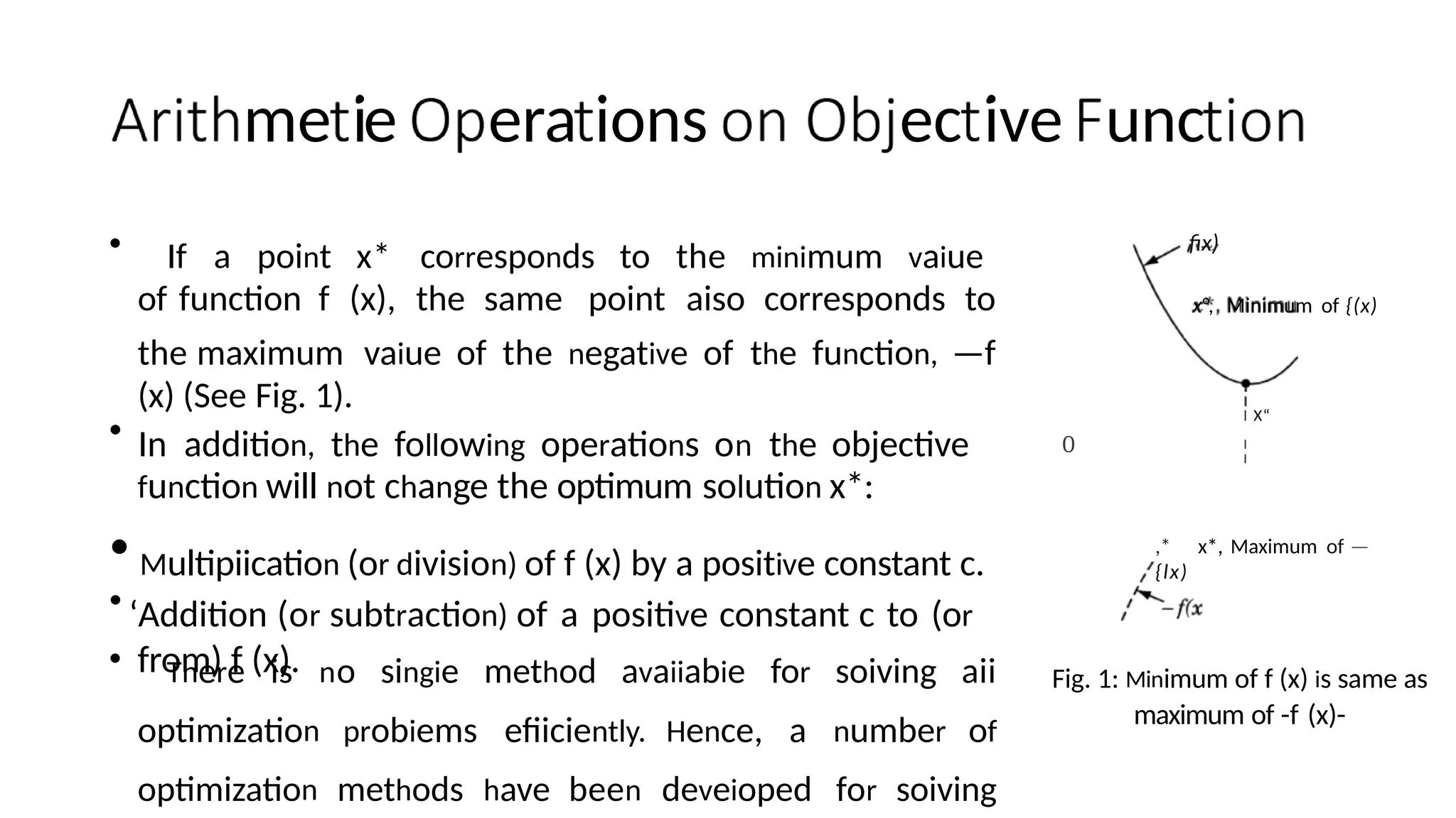
  me ie eraions ec ive unc • If a point x* corresponds to the minimum vaiue of function f (x), the same point aiso corresponds to the maximum vaiue of the negative of the function, —f (x) (See Fig. 1). • In addition, the following operations on the objective function will not change the optimum solution x*: • Multipiication (or division) of f (x) by a positive constant c. • ‘Addition (or subtraction) of a positive constant c to (or from) f (x). • There is no singie method avaiiabie for soiving aii optimization probiems efiiciently. Hence, a number of optimization methods have been deveioped for soiving 0 fix) x°, Minimum of {(x) I X“ I I ,* x*, Maximum of — {lx) Fig. 1: Minimum of f (x) is same as maximum of -f (x)-
• 3.
  ema ica ramminec ues • The optimum seeking methods are also known as mathematical programmingtechniques. • Mathematical programming techniques are useful in finding the minimum of a function of several variables under a prescribed set of constraints. • Statistical methods enable one to analyze the experimental data and build empirical models to obtain the most accurate representation of the physical situation.
• 4.
  0 # , N N , s 0 . 0 1 i i ra i l i ne a r prngrwrnmin Integer proparnmnxng I'*fetwork Ga«ric theory enetic irrtulated arineuliog Particle swarm Neural methods Reliatsility tDenry a I BrCstical rnethc*ds Cluster alysis, pattern Oiscriminate analysis owl yois)
• 5.
  ica ions imiza •*Optimum designof eiectricai networks • *Optimai production pianning, controiiing, and scheduiing • Pianning of maintenance and repiacement of equipment to reduce operatingcosts •Aiiocation of resources or services among severai activities to maximize the benefit °'*Pianning the best strategy to obtain maximum profit in the presence
• 6.
  emen imiza e m • An optimizationor a mathematical programming follows. problem can be stated as where X is an n-dimensional vector called the design vector, f(X) is termed the objective function, and g;(/) and f;(J¢) Find X subject ii) the st›nsir:iiiiis - "/f w hi< h HU131 UJ U c h ( ) 1 j í X 1 Ú. / l . ž . . . . /r (1) • The problem stated in Eq. (1) is called a constrained optimization problem. • Some optimization problems do not involve any constraints and they are called unconstrained optimization problems. are known as inequality and equality constraints, respectively. The number of variables n and the number of inequality and equality constraints m and p, respectively.
• 7.
  esi • Any engineeringsystem or component is defined by a set of quantities some of which are viewed as variables during the design process. • In general, certain quantities are usually fixed at the outset and these are called preassigned parameters. All the other quantities are treated as variables in the design process and are called design or decision variables x;, i 1, 2,...,n. • The design variables are collectively represented as a design vector X (• •› • ••• •z)T • • If an n-dimensional Cartesian space with each coordinate axis representing a design variable x/, i 1, 2,...,n is considered, the space is called the design variable space or simply design space. • Each point in the n-dimensional design space is called a design point
• 8.
  esi rain • In manypractical problems, the design variables cannot be chosen arbitrarily; rather, they have to satisfy certain specified functional and other requirements. • The restrictions that must be satisfied to produce an acceptable design are collectively called design constraints. • Constraints that represent limitations on the behavior or performance of the system are termed behavior or functional constraints. • Constraints that represent physical limitations on design variables, such as availability, fabricability, and transportability, are known as geometric or side constraint.
• 9.
  ons ace • For illustration,consider an optimization problem with only inequality constraints gj(X) 6 0. The set of values of X that satisfy the equation gj(A*) = 0 forms a hypersurface in the design space and is called a constraint surface. • The constraint surface divides the design space into two regions: one in which gj(/¢) < 0 and the other in which gy(7) » 0. • Thus, the points lying on the hypersurface will satisfy the constraint critically, whereas the points lying in the region where gj(A*) > 0 are infeasible or unacceptable, and the points lying in the region where gj(A') < 0 are feasible or acceptable. • The collection of all the constraint surfaces gy(A*) = 0 , j = 1, 2, ... , m, which separates the acceptable region is called the composite constraint surface.
• 10.
  ons ace • Figure showsa hypothetical two-dimensional design space where the infeasible region is indicated by hatched lines. A design point that lies on one or more than one constraint surface is called a bound point, and the associated constraint is called an active constraint. • Design points that do not lie on any constraint surface are known as free points. Depending on whether a particular design point belongs to the acceptable or unacceptable region, it can be identified as one of the following four types: 1. Free and acceptable point 2. Free and unacceptable point 3. Bound and acceptable point 4. Bound and unacceptable point
• 11.
  ons Infeasible region Behavior c‹:nstraint = 0 xFree unacceptable point ace Feasib1y region Bf?hźtviuf c0!"Istrai Flt E — — 0 Side constraint ć3 = o e Free point Bound acceptable poin Behavior Eonstraint S ide constraint,g = g Bound unacceptable polnt Fig-Constraintsurfacesin a hypotheticaitwo-dimensionaidesign
• 12.
  ec ive unc • Theconventional design procedures aim at finding an acceptable or adequate design that merely satisfies the functional and other requirements of the problem. • In general, there will be more than one acceptable design, and the purpose of optimization is to choose the best one of the many acceptable designs available. • Thus, a criterion has to be chosen for comparing the different alternative acceptable designs and for selecting the best one. The criterion with respect to which the design is optimized, when expressed as a function of the design variables, is known as the criterion or merit or objective function. • The choice of objective function is governed by the nature of problem. • In electrical engineering designs, the objective is usually minimization of cost, maximization of profit, etc.
• 13.
  ec ive unc • Thus,the choice of the objective function appears to be straightforward in most design problems. However, there may be cases where the optimization with respect to a particular criterion may lead to results that may not be satisfactory with respect to another criterion. • For example, minimization of network power loss may not correspond to minimum size of capacitor placement. • Thus, the selection of the objective function can be one of the most important decisions in the whole optimum design process. • In some situations, there may be more than one criterion to be satisfied simultaneously. • An optimization problem involving multiple objective functions is known as a
• 14.
  ec ive • Withmuitiple objectives there arises a possibiiity of confiict, and one simpie way to handle the probiem is to construct an overaii objective function as a iinear combination of the confiicting muitipie objective functions. • Thus, i* lb(*) and /2(*) denote two objective functions, construct a new (overaii)objective functionfor optimizationas + 2 * 2 ( ) whP.rIŽ o1 člnd o2 žŽre conStan/is, whose vžŽiUes indiCate thIŽ rP.IativP. importčlnCe of one objective function reiativeto the other.
• 15.
  ec ive unc ace s • Thelocus of all points satisfying f (X) C constant forms a hypersurface in the design space, and each value of C corresponds to a different member of a family of surfaces. These surfaces, called objective function surfaces, are shown in a hypothetical two-dimensional design space in Fig. • Once the objective function surfaces are drawn along with the constraint surfaces, the optimum point can be determined withoutmuch difficulty. • But the main problem is that as the number of design variables exceeds two or three, the constraint and objective function surfaces become complex even for visualization and the problem has to be solved purely as a mathematical problem.
• 16.
  ec ive i aces Fig. Contoursof the objective function