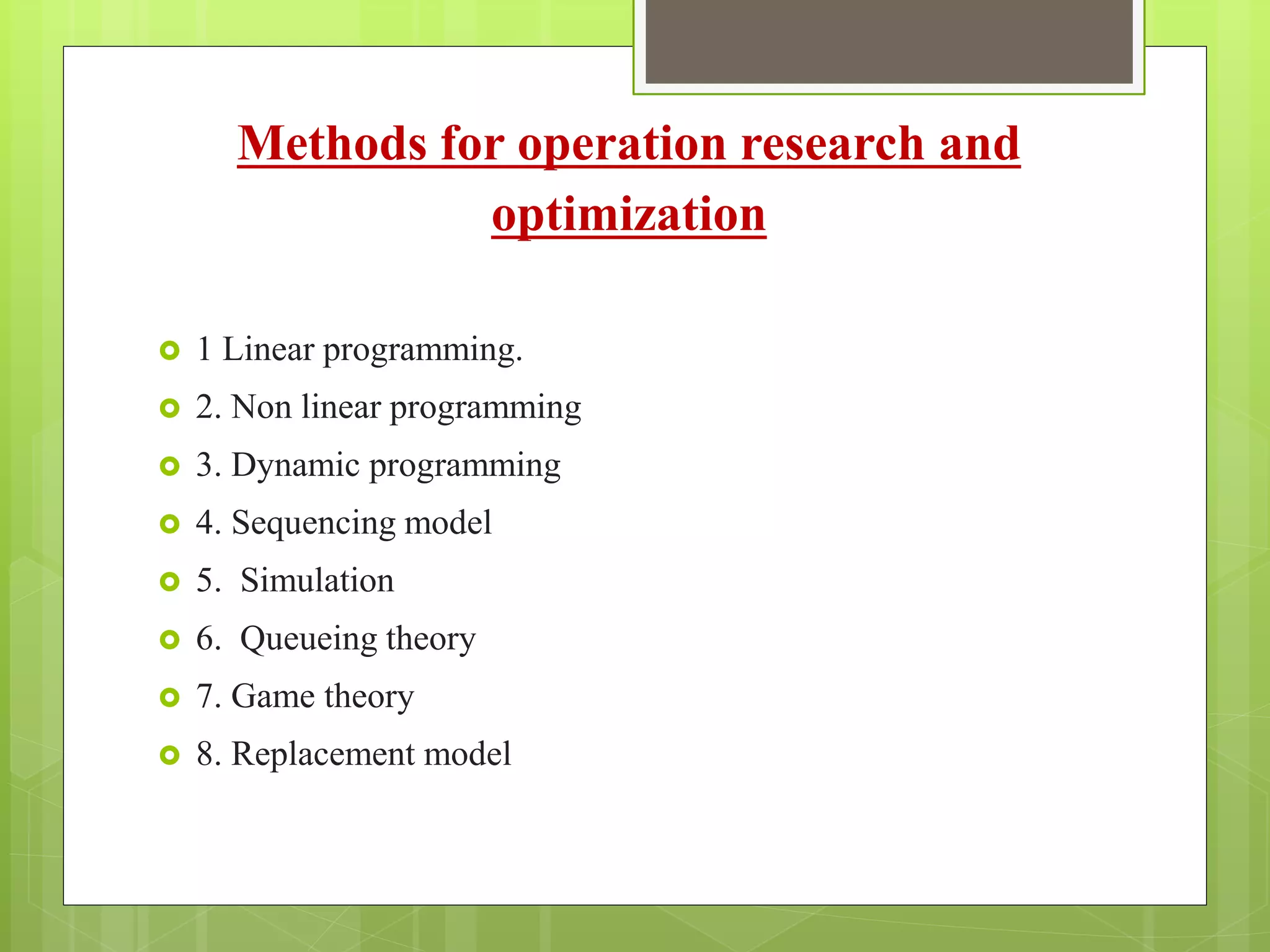
System approach in civil engg slideshare.vvs

System approach in civil engg slideshare.vvs

• 1.
  System Approach inCivil Engineering By Prof. V.V.Sasane Sanjivani College of Engineering, Kopargaon, A.Nagar, Maharashatra
• 2.
  Introduction to Systemapproach  Optimisation: An act, process or methodology of making something (design, system, decision) as fully perfect functional or effective.  System approach: It is a systematic approach towards the problem solving and decision making applying the quantitative methods techniques and tools of optimization.  Engineering application of Optimisation of system approach  1. Design of civil engineering structures such as frames, Foundation bridges Towers chimneys and Dam for minimum cost.  2. Minimum weight design of structure for earthquake, wind and other types of random loading.  3. Design of water resources system.  4. Maximum benefit for optimal plastic design of structure.  5. Optimal production planning controlling and scheduling.  6. Analysis of statistical data and building empirical models from experimental results to obtain the most accurate representation of physical phenomena.  7. Design of optimum pipeline network for water distribution.  8. Selection of site for an industry allocation of resources or services among several activities to maximize the benefit.  9. Planning the best strategy to obtain maximum profit in presence of competitor.  10. Inventory control
• 3.
  Civil engineering applicationof optimisation or system approach  1. Design of civil engineering structures such as frames, Foundation bridges Towers chimneys and Dam for minimum cost.  2. Minimum weight design of structure for earthquake, wind and other types of random loading.  3. Design of water resources system.  4. Maximum benefit for optimal plastic design of structure.  5. Optimal production planning controlling and scheduling.  6. Analysis of statistical data and building empirical models from experimental results to obtain the most accurate representation of physical phenomena.  7. Design of optimum pipeline network for water distribution.  8. Selection of site for an industry allocation of resources or services among several activities to maximize the benefit.  9. Planning the best strategy to obtain maximum profit in presence of competitor.  10. Inventory control
• 4.
  Methods for operationresearch and optimization  1 Linear programming.  2. Non linear programming  3. Dynamic programming  4. Sequencing model  5. Simulation  6. Queueing theory  7. Game theory  8. Replacement model
• 5.
  Important Terms  Linearprogramming:  Linear programming deals with optimisation (maximization and minimization) of a function of variables known as an objective function subject to a set of linear equation and inequalities known constraints. By linearity it means a mathematical expression in which the expressions among the variable are linear example, a1 x1 + a2 x2 + …… + a n x n is linear higher powers of the variable or their products do not appear in the expression of objective function as well as constraint the variables obey the properties of proportionality and additivity.  Nonlinear programming: By non linearity it means a mathematical expression in which the expression among the variable or nonlinear e.g. a1x1 +a3x2 2 +a2x1x2. Higher powers of the variables and their products may appear in the expression of objective function as well as in the constraint the variables do not obey the properties of proportionality and additivity  Objective function: The criteria with respect to which the design is optimised, when expressed as a function of design variable is known as objective function Objective function may be profit, cost, production capacity or any other Major of effectiveness .  Constraint: Constraint is the element, factor of a subsystem that restricts an entity, project or system from achieving its goal.  Or  Mathematical expression of the limitation on the fulfillment of objectives. Constraint may be imposed by the different resources such as market demand, production process and equipment, storage capacity from a raw material availability etc.
• 6.
  Local and Globaloptimum  In nonlinear programming, a function may have more than one maxima or minima values. That is when the function is plotted, it has more than one Peak or more than one Valley. Each of these is local maximum or local minimum. Global or absolute maximum of the function is the value higher than all the values of the function similarly a global minimum of a function is a value which is the lowest of all the values of function.
• 7.
   Consider thesingle variable function plotted in above figure over the interval x = a and x = b, this function has three local Maxima x 1, x 3 and x 7. The global maxima is at x 7 similarly, there are three local minima at x 2, x 4 and x 6. The global minima is f (x 7) at x = x 7. Point corresponding to x5 which has zero slope is called point of inflation. If the point with zero slope is not maximum or minimum then it must automatically be and inflation point or a saddle point. Global Maximum Saddle Point or Global Minimum Point of Inflation a x1 x2 x3 x4 x5 x6 x7 b x F(x)
• 8.
  Concave and convexfunction  Concave Function:  A single variable function, which when plotted results in a curve, always coming down word or not coming at all is called concave function figure below shows a single variable concave function the shape of this function is such that for any two points on the curve in the feasible region S. the line joining the point is always below the function. It is clear from the figure that there is always a unique global maximum of such a functions.  It can be shown from concave function of several variables, that if it has a local maximum the same is also its Global maximum a function f (x) is said to be concave over a region if any two points x and y in S.  , Where  10         yfxfyxf   1)(1 ,
• 9.
   Convex Function: A function which when plotted result in a always curving upward or not curving at all is called convex function. figure below shows a single variable convex function. A line joining any two points on the curve in the feasible region S is always above the function, there is always a unique global minimum of a several function. For a convex function of several variables if there exist a local minimum, it can be proved that the same is also the global minimum.  In mathematical form       yfxfyxf   1)(1 , Where 10  
• 10.
  Numerical  Statement:For thefollowing functions determine whether it is concave or convex. a. f(x) = x1x2-x1 2-x2 2 b. f(x) = 3x1 + 2x1 2 + 4x2+ x2 2 – 2x1x2  Solution: a. f(x) = x1x2-x1 2 -x2 2 1x f   = x2 – 2x1 and 2 1 2 x f   = -2 which ≤ 0 2x f   = x1 – 2x2 and 2 2 2 x f   = -2 which ≤ 0 21 2 xx f   = 1 2 1 2 x f   - 2 2 2 x f   - [ 21 2 xx f   ] = (-2) (-2) –(1)2 =3 which is ≥ 0 Therefore function is strictly concave.
• 11.
  a. f(x)=3x1 +2x1 2 +4x2+x2 2 –2x1x2 1x f   =3+4x1-2x2;2 1 2 x f   =4 ≥0 2x f   =4+2x2-2x1; and 2 2 2 x f   = 2≥0 21 2 xx f   =-2 2 1 2 x f   - 2 2 2 x f   -[ 21 2 xx f   ]=(4)(2)–(-2)2 =4≥0 Thereforethe functionstrictlyconvex
• 12.
  Thank You !