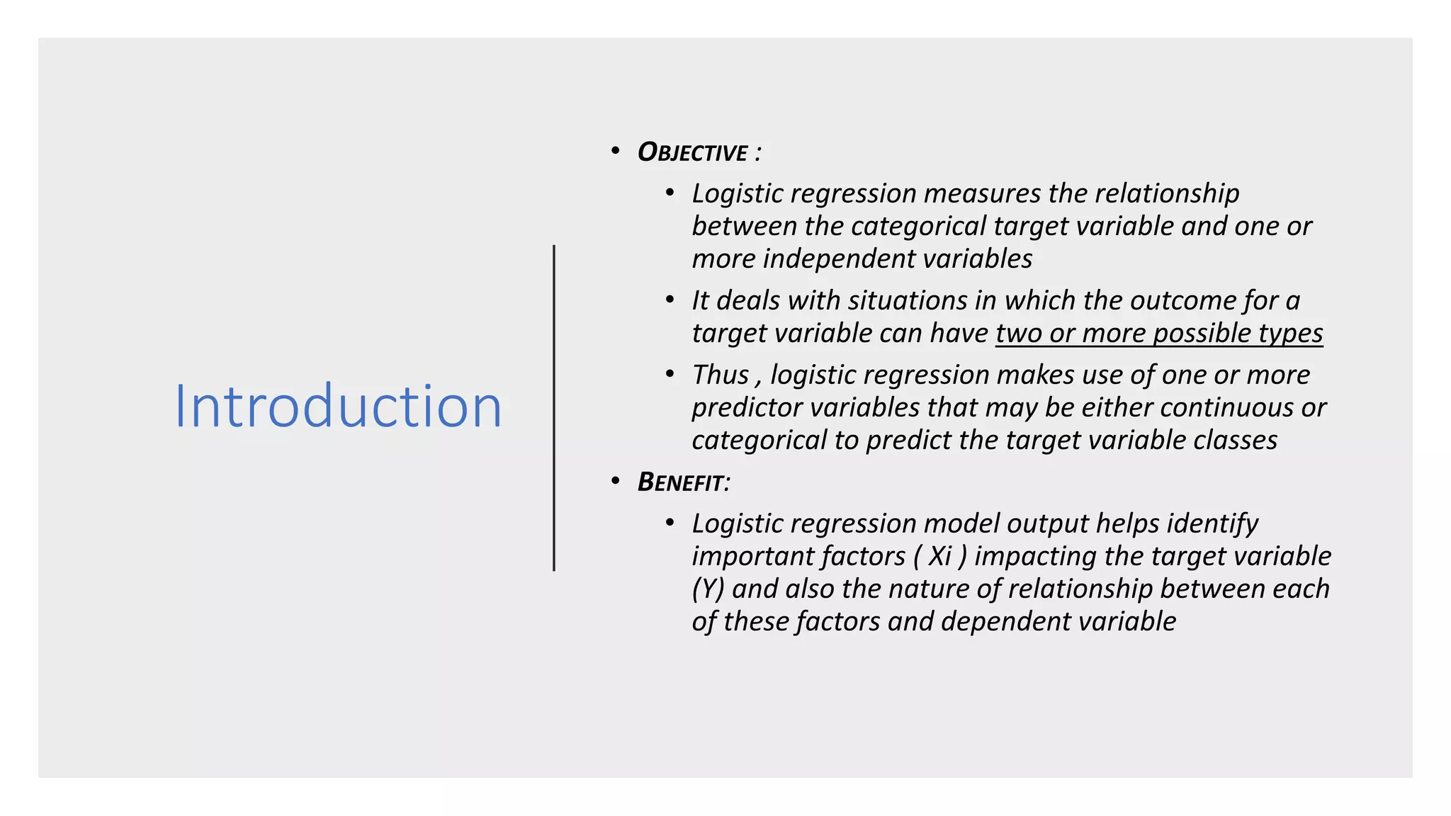
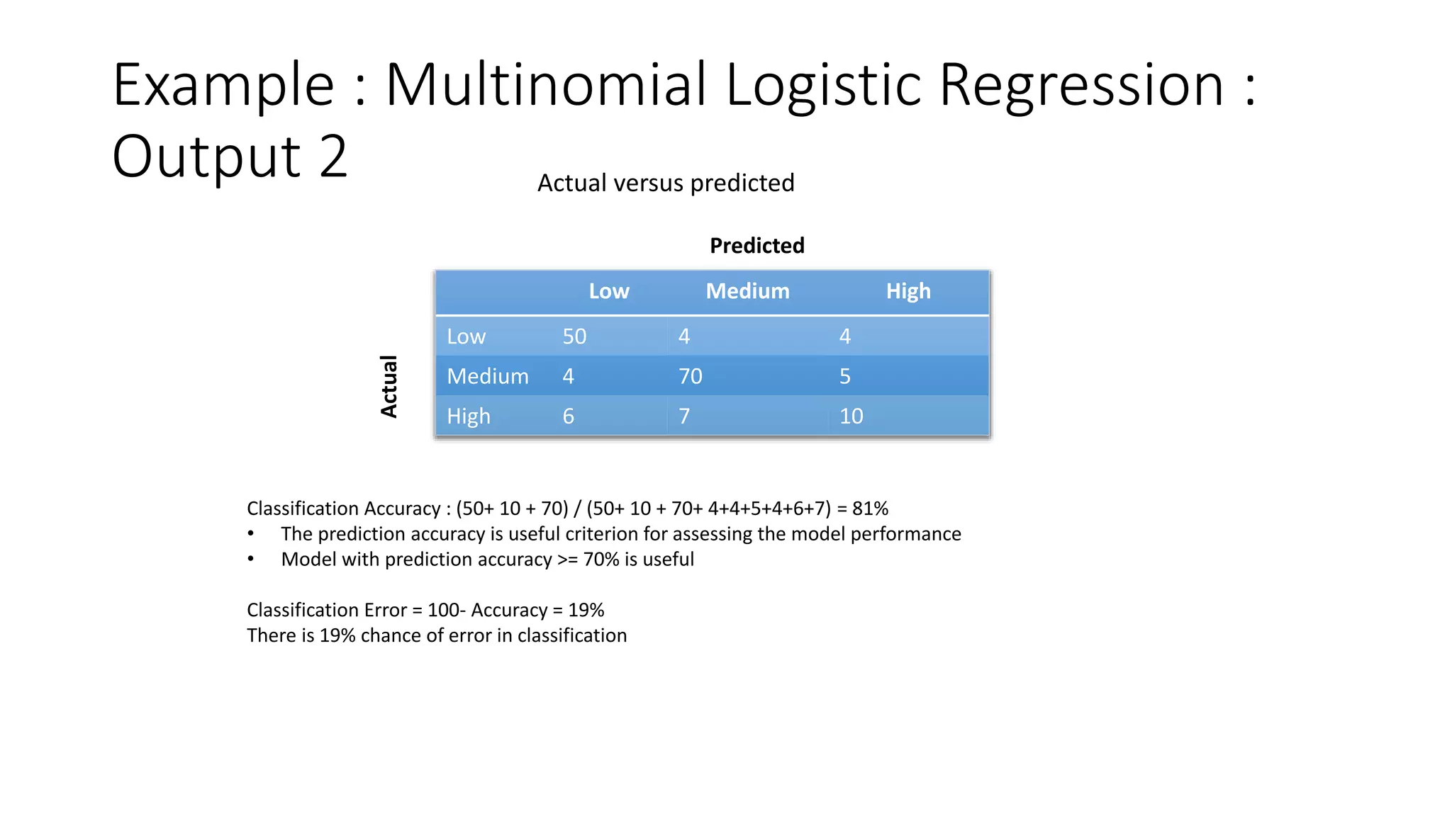
Master the Art of Analytics
A Simplistic Explainer Series For Citizen Data Scientists
J o u r n e y To w a r d s A u g m e n t e d A n a l y t i c s
Multinomial Logistic
Regression
Terminologies
Introduction & Example
Standard input/tuning parameters & Sample UI
Sample output UI
Interpretation of Output
Limitations
Business use cases
What Are
All Covered
Terminologies
Terminologies
 Target variable usually denoted by Y , is the variable being predicted and is also
called dependent variable, output variable, response variable or outcome
variable (Ex : One highlighted in red box in table below)
 Predictor, sometimes called an independent variable, is a variable that is being
used to predict the target variable ( Ex : variables highlighted in green box in
table below )
Age Marital Status Gender
Satisfaction
level
58 married Female High
44 single Female Low
33 married Male Medium
47 married Female High
33 single Female Medium
35 married Male High
28 single Male Low
Introduction & Example
Introduction
• OBJECTIVE :
• Logistic regression measures the relationship
between the categorical target variable and one or
more independent variables
• It deals with situations in which the outcome for a
target variable can have two or more possible types
• Thus , logistic regression makes use of one or more
predictor variables that may be either continuous or
categorical to predict the target variable classes
• BENEFIT:
• Logistic regression model output helps identify
important factors ( Xi ) impacting the target variable
(Y) and also the nature of relationship between each
of these factors and dependent variable
Example : Multinomial Logistic Regression :
Input Let’s conduct the Multinomial Logistic Regression analysis on following variables :
Job satisfaction
level
Age Marital Status Gender Income
Low 58 married Male 46,399
Medium 44 single Male 47,971
Low 33 married Female 52,618
High 47 married Male 28,717
Medium 33 single Female 41,216
Medium 35 married Female 34,372
Low 28 single Male 64,811
Medium 42 divorced Female 53,000
High 58 married Female 41,375
Low 43 single Male 53,778
Low 41 divorced Male 44,440
Medium 29 single Female 51,026
Independent variables (Xi)Target Variable (Y)
Example : Multinomial Logistic Regression :
Output 1 Coefficient P value
High
Age 1.54 0.05
Income -0.34 0.03
Male 0.67 0.02
Low
Age -2.34 0.05
Income 0.56 0.01
Male -1.23 0.04
Coefficients
• High satisfaction with reference to medium satisfaction:
Age - Multinomial logit (Natural log of the proportion of High to that of Medium here)
estimate for 1 year increase in age for high job satisfaction relative to medium job satisfaction
when other independent variables are held constant = 1.54
Male - Multinomial logit estimate for comparing male to females for high job
satisfaction relative to medium job satisfaction when other variables are held constant = 0.67
Interpretation
Example : Multinomial Logistic Regression :
Output 2
Classification Accuracy : (50+ 10 + 70) / (50+ 10 + 70+ 4+4+5+4+6+7) = 81%
• The prediction accuracy is useful criterion for assessing the model performance
• Model with prediction accuracy >= 70% is useful
Classification Error = 100- Accuracy = 19%
There is 19% chance of error in classification
Low Medium High
Low 50 4 4
Medium 4 70 5
High 6 7 10
Actual versus predicted
Predicted
Actual
Standard input/tuning
parameters & Sample
UI
STANDARD
INPUT
PARAMETERS
& SAMPLE UI
SAMPLE OUTPUT UI
Sample output 1 : Model Summary
Actual versus predicted
Predicted
Actual
Coefficient matrix :
Low Medium High
Low 50 4 4
Medium 4 70 5
High 6 7 10
Coefficient P value
High
Age 1.54 0.05
Income -0.34 0.03
Male 0.67 0.02
Low
Age -2.34 0.05
Income 0.56 0.01
Male -1.23 0.04
Age Marital Status Gender Income
Job satisfaction
level
Predicted
class
Probability
58 married Female 46,399 Low Low 0.7
44 single Female 47,971 High High 0.9
33 married Male 52,618 Low Low 0.8
47 married Female 28,717 Low High 0.7
33 single Male 41,216 High Low 0.6
35 married Male 34,372 High High 0.5
28 single Female 64,811 Low Low 0.4
42 divorced Male 53,000 Low Low 0.3
58 married Female 41,375 High Low 0.2
43 single Male 53,778 High High 0.1
Sample output 2 : Predicted class &
probability
Sample Output 3 : Classification Plot
• Lesser the overlap among three classes in the plot above , better the classification done
by model
• Thus, output will contain predicted class column, confusion matrix and classification plot
Interpretation of
Output
Interpretation of Important Model Summary
Statistics
Accuracy:
 If Accuracy >= 70% : Model is well fit on
provided data and predicted classes are
reasonably accurate
 If Accuracy < 70% : Model is not well fit on
provided data and predicted classes are
likely to contain high chances of error
Coefficients and p value :
 If value of coefficient is positive and p value
<0.05 , variable is positively correlated with target
variable
 If value of coefficient is negative and p value
<0.05 , variable is negatively correlated with
target variable
 If p value > 0.05, variable is unimportant in terms
of predicting target variable classes
Limitations
Limitations
 It is applicable only when target variable is categorical
 Sample size must be at least 1000 in order to get reliable predictions
 Level 1 of the target variable should represent the desired outcome.
 i.e. if desired class is yes in response/non response target variable
then Yes has to be recoded into 1 and No into 0
Business Use Cases
Use case 1
Business benefit:
• By having a knowledge of probable
election outcome, proper strategy
can be put in place in case of
discrepancies between
expectations and predictions and
the segments with high likelihood
of voting oppositions can be
targeted in better and effective
manner in order to get their votes
in favor of a client party
Business problem :
• A research agency wants to predict
the likelihood of each election
candidate being voted by each
voter and in turn devise a strategy
to take proactive steps
• Here the target variable would be
‘preferred party name’ and
predictors would be customer
demographics such as age, income,
qualification, occupation, gender,
religion and past voting status etc.
Use case 1 : Sample Input Dataset
Responder
ID
Qualification income Age Gender Occupation
Done voting in
past
Preferred party
1039153 Bcom 105000 18 M Accountant yes ABC
1069697 12th
Pass 192000 20 F
Office
Supervisor
No XYZ
1068120 BSC 310000 30 F Pathologist yes PQL
563175 10th
Pass 100000 45 M Labour yes XYZ
562842 ME 357228 25 M
Software
Developer
No PQL
562681 MSC 413000 28 F Statistician yes XYZ
562404 BSC Nill 34 F Home maker No PQL
Use case 1 : Output : Predicted Class
Output : Each record will have a predicted class along with probability assigned as
shown below :
Respond
er ID
Qualificatio
n
Income Age Gender Occupation
Done
voting in
past
Predicted
party
Probability
1039153 Bcom 105000 18 M Accountant yes ABC 0.7
1069697 12th
Pass 192000 20 F
Office
Supervisor
No XYZ 0.9
1068120 BSC 310000 30 F Pathologist yes PQL 0.8
563175 10th
Pass 100000 45 M Labour yes XYZ 0.7
562842 ME 357228 25 M
Software
Developer
No PQL 0.6
562681 MSC 413000 28 F Statistician yes XYZ 0.5
562404 BSC Nill 34 F
Home
maker
No PQL 0.4
Use case 1 : Output : Sample Class profile
Predicted
Party
Average
Annual
income
Average
Age
ABC 86,467 30
XYZ 60,935 25
PQL 1,05,400 35
• As can be seen in the table above, there is distinctive characteristics of population associated with each preferred
party :
• For instance, females are inclined towards XYZ whereas males tend to prefer ABC
• Responders with high income and age prefer to vote for PQL whereas XYZ party is preferred by lowest income and
age group
• Fresh voters are likely to vote for party XYZ whereas those who have done voting in past are inclined towards ABC
party
Gender
Predicted
Party
Male Female
ABC 60 4
XYZ 10 78
PQL 14 15
Past voting status
Predicted
Party
Yes No
ABC 58 6
XYZ 15 73
PQL 11 19
Use case 2
Business benefit:
•Given the body profile of a patient
and predicted level of disease , right
cure/medications can be suggested to
a patient
Business problem :
•A doctor/ pharmacist wants to predict
the likelihood of a new patient’s
disease being at
initial/intermediate/severe stage
based on various body attributes of a
patient such as blood pressure ,
hemoglobin level, sugar level , red
blood counts, TSH etc.
•Here the target variable would be level
of disease and would contain values
‘Initial, Intermediate and Severe’
Want to Learn
More?
Get in touch with us @
support@Smarten.com
And Do Checkout the Learning section
on
Smarten.com
June 2018

What is the Multinomial-Logistic Regression Classification Algorithm and How Does One Use it for Analysis?

  • 1.
    Master the Artof Analytics A Simplistic Explainer Series For Citizen Data Scientists J o u r n e y To w a r d s A u g m e n t e d A n a l y t i c s
  • 2.
  • 3.
    Terminologies Introduction & Example Standardinput/tuning parameters & Sample UI Sample output UI Interpretation of Output Limitations Business use cases What Are All Covered
  • 4.
  • 5.
    Terminologies  Target variableusually denoted by Y , is the variable being predicted and is also called dependent variable, output variable, response variable or outcome variable (Ex : One highlighted in red box in table below)  Predictor, sometimes called an independent variable, is a variable that is being used to predict the target variable ( Ex : variables highlighted in green box in table below ) Age Marital Status Gender Satisfaction level 58 married Female High 44 single Female Low 33 married Male Medium 47 married Female High 33 single Female Medium 35 married Male High 28 single Male Low
  • 6.
  • 7.
    Introduction • OBJECTIVE : •Logistic regression measures the relationship between the categorical target variable and one or more independent variables • It deals with situations in which the outcome for a target variable can have two or more possible types • Thus , logistic regression makes use of one or more predictor variables that may be either continuous or categorical to predict the target variable classes • BENEFIT: • Logistic regression model output helps identify important factors ( Xi ) impacting the target variable (Y) and also the nature of relationship between each of these factors and dependent variable
  • 8.
    Example : MultinomialLogistic Regression : Input Let’s conduct the Multinomial Logistic Regression analysis on following variables : Job satisfaction level Age Marital Status Gender Income Low 58 married Male 46,399 Medium 44 single Male 47,971 Low 33 married Female 52,618 High 47 married Male 28,717 Medium 33 single Female 41,216 Medium 35 married Female 34,372 Low 28 single Male 64,811 Medium 42 divorced Female 53,000 High 58 married Female 41,375 Low 43 single Male 53,778 Low 41 divorced Male 44,440 Medium 29 single Female 51,026 Independent variables (Xi)Target Variable (Y)
  • 9.
    Example : MultinomialLogistic Regression : Output 1 Coefficient P value High Age 1.54 0.05 Income -0.34 0.03 Male 0.67 0.02 Low Age -2.34 0.05 Income 0.56 0.01 Male -1.23 0.04 Coefficients • High satisfaction with reference to medium satisfaction: Age - Multinomial logit (Natural log of the proportion of High to that of Medium here) estimate for 1 year increase in age for high job satisfaction relative to medium job satisfaction when other independent variables are held constant = 1.54 Male - Multinomial logit estimate for comparing male to females for high job satisfaction relative to medium job satisfaction when other variables are held constant = 0.67 Interpretation
  • 10.
    Example : MultinomialLogistic Regression : Output 2 Classification Accuracy : (50+ 10 + 70) / (50+ 10 + 70+ 4+4+5+4+6+7) = 81% • The prediction accuracy is useful criterion for assessing the model performance • Model with prediction accuracy >= 70% is useful Classification Error = 100- Accuracy = 19% There is 19% chance of error in classification Low Medium High Low 50 4 4 Medium 4 70 5 High 6 7 10 Actual versus predicted Predicted Actual
  • 11.
  • 12.
  • 13.
  • 14.
    Sample output 1: Model Summary Actual versus predicted Predicted Actual Coefficient matrix : Low Medium High Low 50 4 4 Medium 4 70 5 High 6 7 10 Coefficient P value High Age 1.54 0.05 Income -0.34 0.03 Male 0.67 0.02 Low Age -2.34 0.05 Income 0.56 0.01 Male -1.23 0.04
  • 15.
    Age Marital StatusGender Income Job satisfaction level Predicted class Probability 58 married Female 46,399 Low Low 0.7 44 single Female 47,971 High High 0.9 33 married Male 52,618 Low Low 0.8 47 married Female 28,717 Low High 0.7 33 single Male 41,216 High Low 0.6 35 married Male 34,372 High High 0.5 28 single Female 64,811 Low Low 0.4 42 divorced Male 53,000 Low Low 0.3 58 married Female 41,375 High Low 0.2 43 single Male 53,778 High High 0.1 Sample output 2 : Predicted class & probability
  • 16.
    Sample Output 3: Classification Plot • Lesser the overlap among three classes in the plot above , better the classification done by model • Thus, output will contain predicted class column, confusion matrix and classification plot
  • 17.
  • 18.
    Interpretation of ImportantModel Summary Statistics Accuracy:  If Accuracy >= 70% : Model is well fit on provided data and predicted classes are reasonably accurate  If Accuracy < 70% : Model is not well fit on provided data and predicted classes are likely to contain high chances of error Coefficients and p value :  If value of coefficient is positive and p value <0.05 , variable is positively correlated with target variable  If value of coefficient is negative and p value <0.05 , variable is negatively correlated with target variable  If p value > 0.05, variable is unimportant in terms of predicting target variable classes
  • 19.
  • 20.
    Limitations  It isapplicable only when target variable is categorical  Sample size must be at least 1000 in order to get reliable predictions  Level 1 of the target variable should represent the desired outcome.  i.e. if desired class is yes in response/non response target variable then Yes has to be recoded into 1 and No into 0
  • 21.
  • 22.
    Use case 1 Businessbenefit: • By having a knowledge of probable election outcome, proper strategy can be put in place in case of discrepancies between expectations and predictions and the segments with high likelihood of voting oppositions can be targeted in better and effective manner in order to get their votes in favor of a client party Business problem : • A research agency wants to predict the likelihood of each election candidate being voted by each voter and in turn devise a strategy to take proactive steps • Here the target variable would be ‘preferred party name’ and predictors would be customer demographics such as age, income, qualification, occupation, gender, religion and past voting status etc.
  • 23.
    Use case 1: Sample Input Dataset Responder ID Qualification income Age Gender Occupation Done voting in past Preferred party 1039153 Bcom 105000 18 M Accountant yes ABC 1069697 12th Pass 192000 20 F Office Supervisor No XYZ 1068120 BSC 310000 30 F Pathologist yes PQL 563175 10th Pass 100000 45 M Labour yes XYZ 562842 ME 357228 25 M Software Developer No PQL 562681 MSC 413000 28 F Statistician yes XYZ 562404 BSC Nill 34 F Home maker No PQL
  • 24.
    Use case 1: Output : Predicted Class Output : Each record will have a predicted class along with probability assigned as shown below : Respond er ID Qualificatio n Income Age Gender Occupation Done voting in past Predicted party Probability 1039153 Bcom 105000 18 M Accountant yes ABC 0.7 1069697 12th Pass 192000 20 F Office Supervisor No XYZ 0.9 1068120 BSC 310000 30 F Pathologist yes PQL 0.8 563175 10th Pass 100000 45 M Labour yes XYZ 0.7 562842 ME 357228 25 M Software Developer No PQL 0.6 562681 MSC 413000 28 F Statistician yes XYZ 0.5 562404 BSC Nill 34 F Home maker No PQL 0.4
  • 25.
    Use case 1: Output : Sample Class profile Predicted Party Average Annual income Average Age ABC 86,467 30 XYZ 60,935 25 PQL 1,05,400 35 • As can be seen in the table above, there is distinctive characteristics of population associated with each preferred party : • For instance, females are inclined towards XYZ whereas males tend to prefer ABC • Responders with high income and age prefer to vote for PQL whereas XYZ party is preferred by lowest income and age group • Fresh voters are likely to vote for party XYZ whereas those who have done voting in past are inclined towards ABC party Gender Predicted Party Male Female ABC 60 4 XYZ 10 78 PQL 14 15 Past voting status Predicted Party Yes No ABC 58 6 XYZ 15 73 PQL 11 19
  • 26.
    Use case 2 Businessbenefit: •Given the body profile of a patient and predicted level of disease , right cure/medications can be suggested to a patient Business problem : •A doctor/ pharmacist wants to predict the likelihood of a new patient’s disease being at initial/intermediate/severe stage based on various body attributes of a patient such as blood pressure , hemoglobin level, sugar level , red blood counts, TSH etc. •Here the target variable would be level of disease and would contain values ‘Initial, Intermediate and Severe’
  • 27.
    Want to Learn More? Getin touch with us @ support@Smarten.com And Do Checkout the Learning section on Smarten.com June 2018