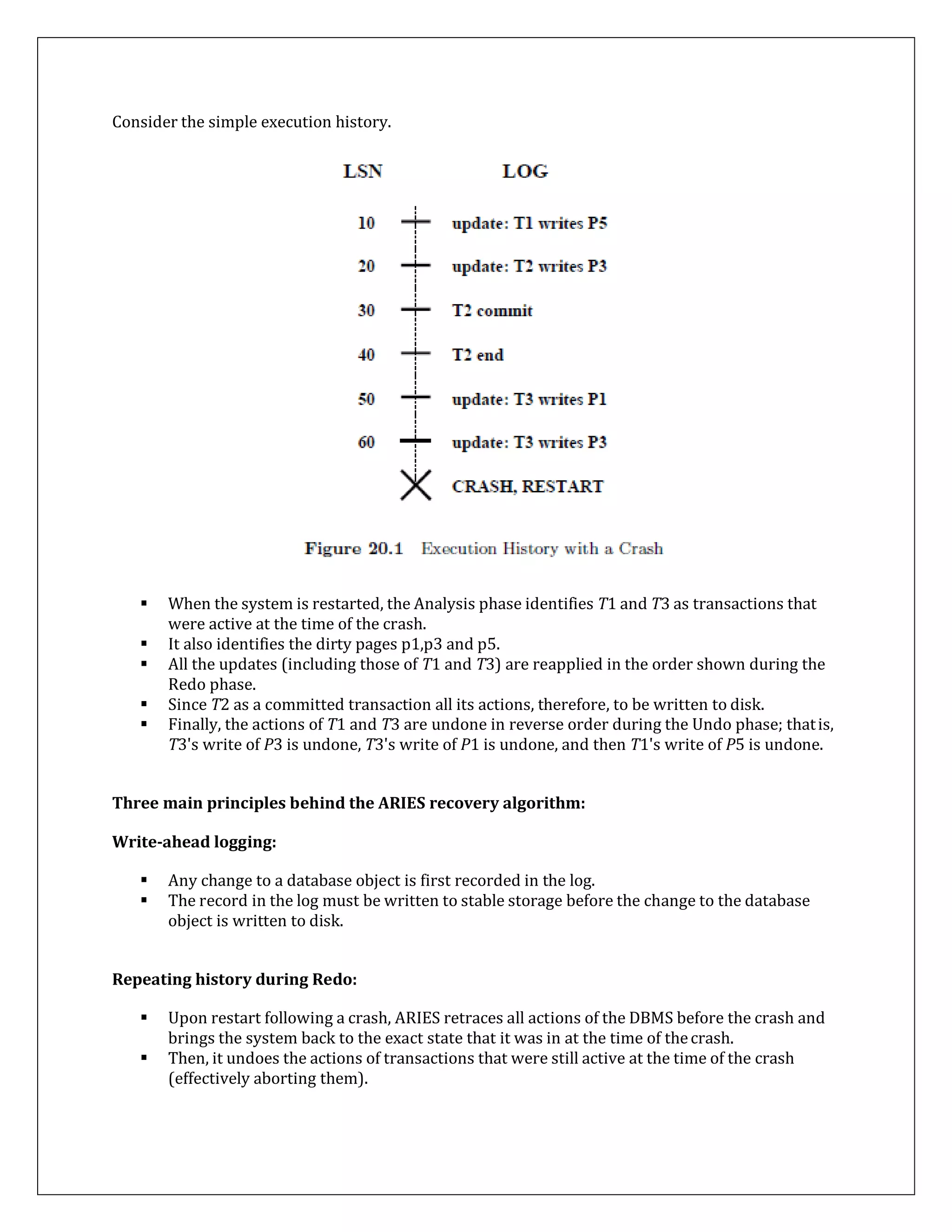
Downloaded 45 times
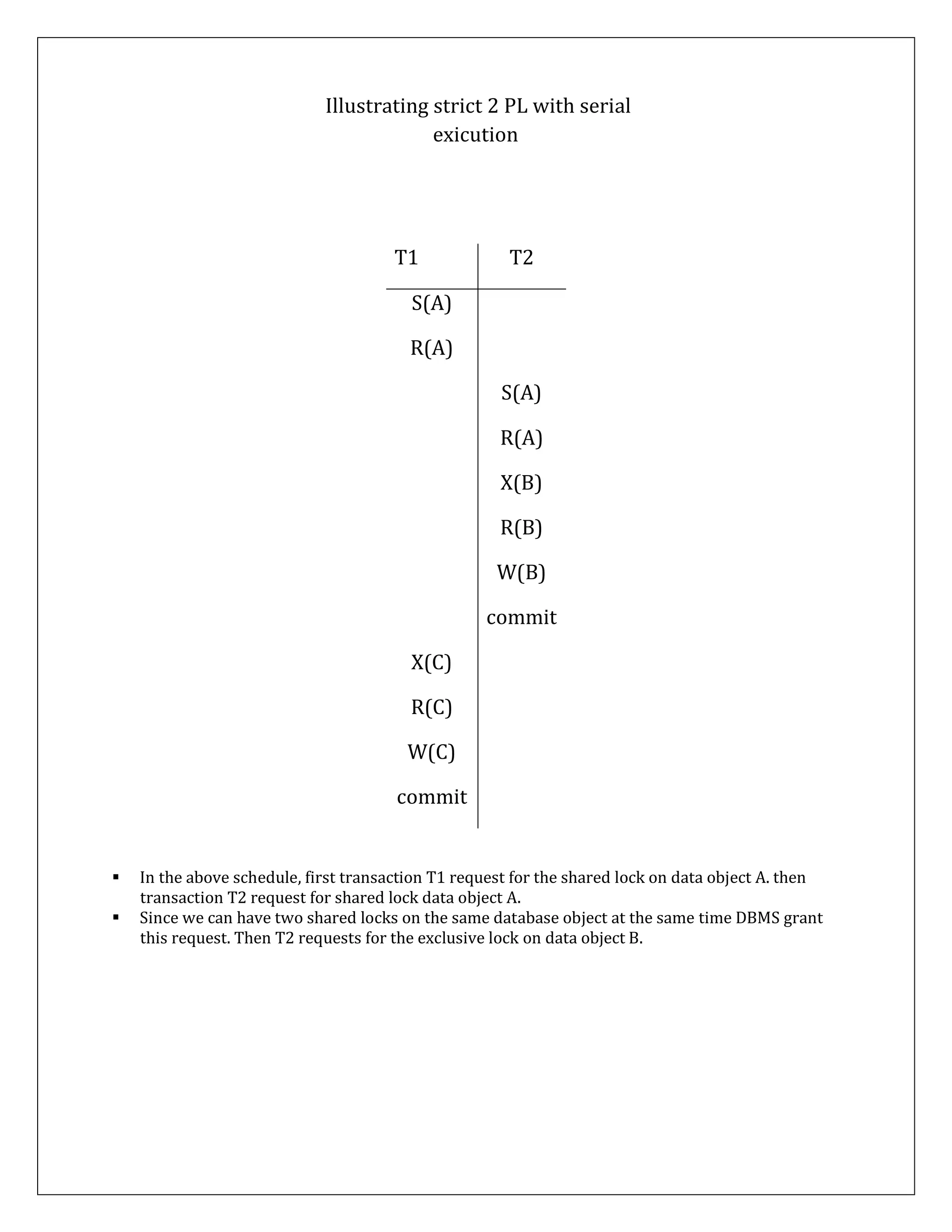
![ But in the meantime, another transaction might have requested and received a conflicting
lock!
To prevent this, the entire sequence of actions in a lock request call (checking to see if the
request can be granted, updating the lock table, etc.) must be implemented as an atomic
operation.
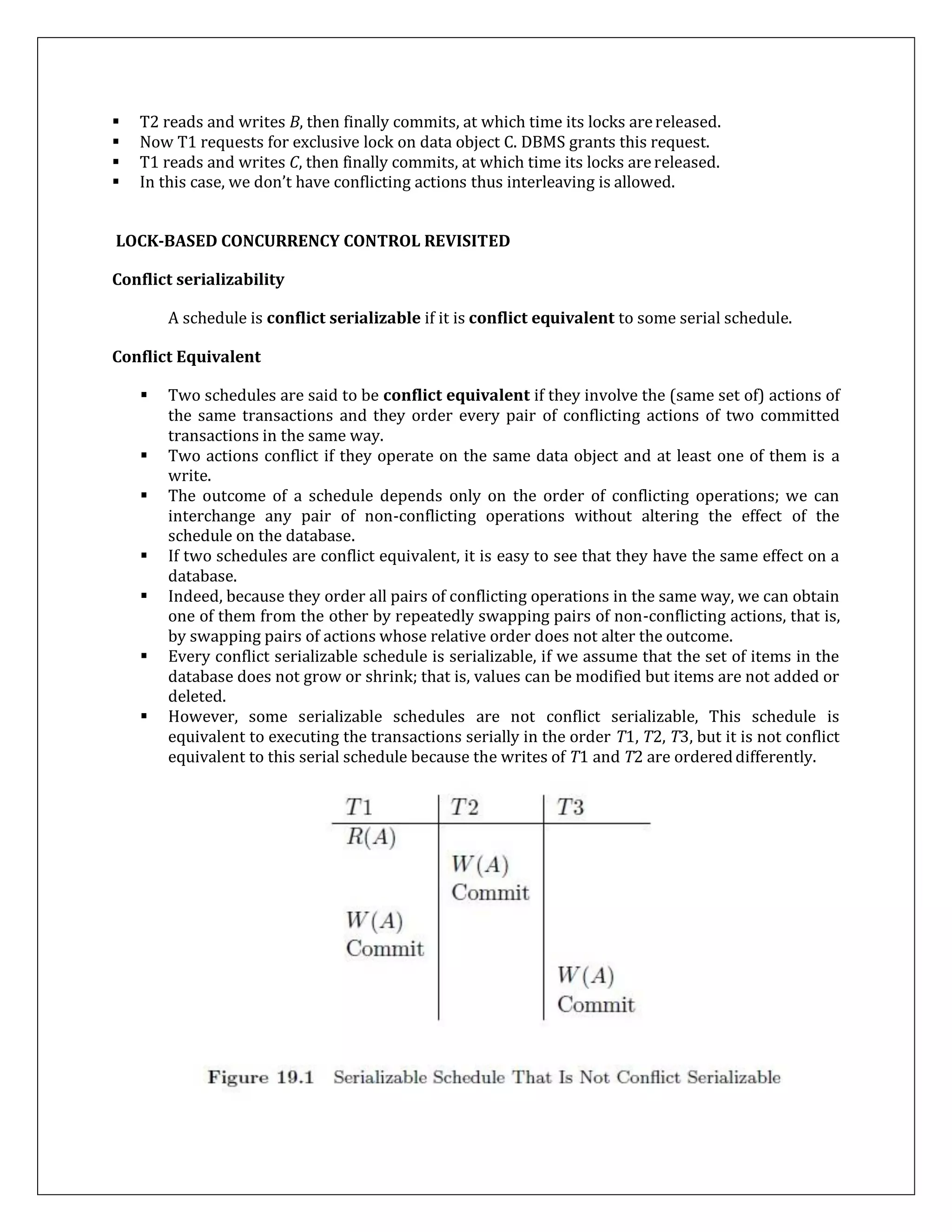
LOCK Conversions
The DBMS maintains a transaction table, which contains (among other things) a list of the
locks currently held by a transaction.
This list can be checked before requesting a lock, to ensure that the same transaction does
not request the same lock twice.
However, a transaction may need to acquire an exclusive lock on an object for which it
already holds a shared lock. Such a lock upgrade request is handled specially by granting
the write lock immediately if no other transaction holds a shared lock on the object and
inserting the request at the front of the queue otherwise.
The rationale for favoring the transaction thus is that it already holds a shared lock on the
object and queuing it behind another transaction that wants an exclusive lock on the same
object causes both transactions to wait for each other and therefore be blockedforever.
Lock upgrades leads to a deadlocks caused by conflicting upgrade requests.
For example, , if two transactions that hold a shared lock on an object both request an
upgrade to an exclusive lock, this leads to a deadlock because first transaction is waiting for
second to release its lock and other transaction is waiting for first transaction to release its
lock.]
A better approach is to avoid the need for lock upgrades altogether by obtaining exclusive
locks initially and downgrading to a shared lock once it is clear that this issufficient.
For example of an SQL update statement, rows in a table are locked in exclusive mode first.
If a row does not satisfy the condition for being updated, the lock on the row is downgraded
to a shared lock.
The downgrade approach reduces concurrency by obtaining white lock some cases where
they are not require.
On the whole require, however, it improve through put by reducing dead locks.
This approach is therefore widely used current commercial system.
Concurrency can be increase by introducing new kind of lock, called and update lock that is
compatible with shared lock but not other update and exclusive lock.
By setting and update lock initially, rather than exclusive lock, we prevent conflict with read
operation.
Once we are sure we need not update object, we can downgrade to the shared lock.
If we need to update the object, we must first upgrade to an exclusive lock. This upgrade
does not lead to a deadlock because no other transaction can have an upgrade or exclusive
on the object.
Additional Issues: Lock Upgrades, Convoys, Latches
We have concentrated thus far on how the DBMS schedules transactions, based on their
requests for locks. This interleaving interacts with the operating system's scheduling of
processes access to the CPU and can lead to a situation called a convoy, where most of the
CPU cycles are spent on process switching. The problem is that a transaction T holding a](https://image.slidesharecdn.com/tybsc-csdbms2notes-170810043037/75/Tybsc-cs-dbms2-notes-21-2048.jpg)
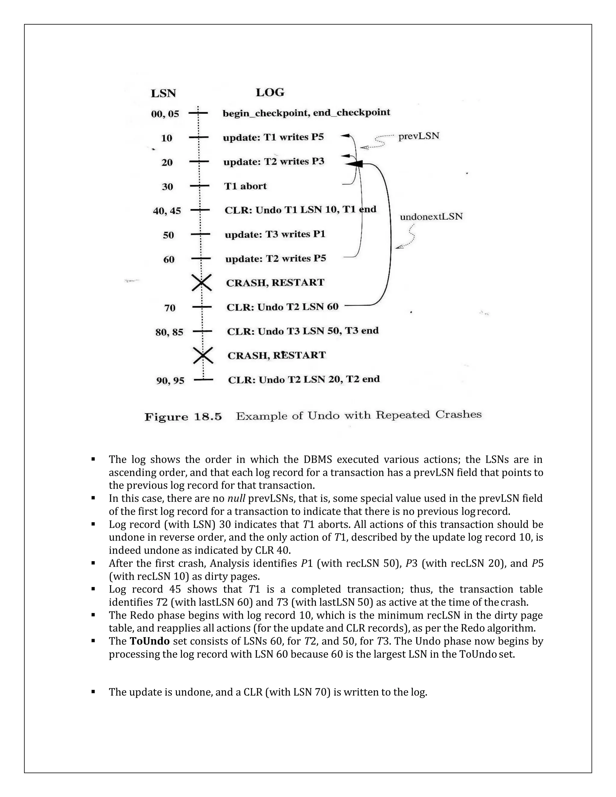
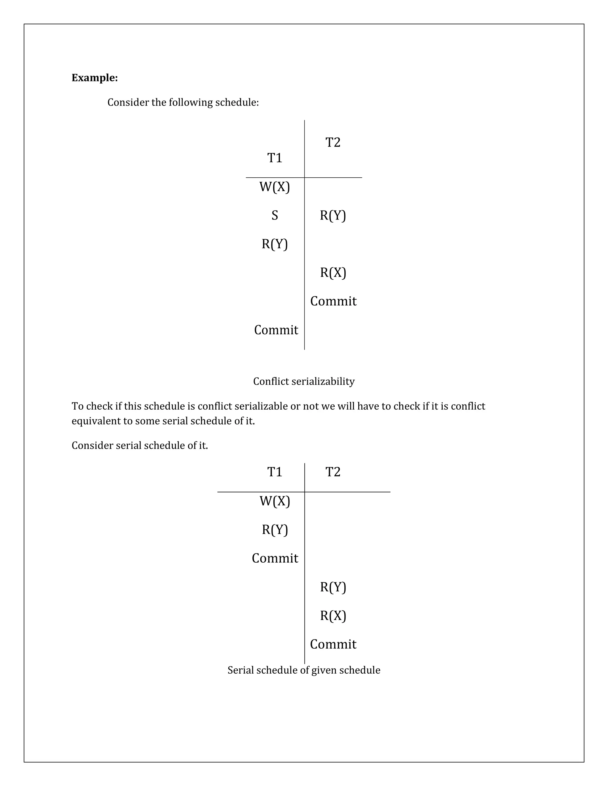
![ORDER / NOORDER]
Note: - Sequence is always given a name so that it can be referenced later when required.
Keywords And Parameters
INCREMENT BY: Specifies the interval between sequence numbers. It can be any positive or
negative value but not zero. If this clause is omitted, the default value is 1.
MINVALUE: Specifies the sequence minimum value.
NOMINVALUE: Specifies a minimum value of 1 for an ascending sequence and -(10)^26 for a
descending sequence.
MAXVALUE: Specifics the maximum value that a sequence can generate.
NOMAXVALUE: Specifies a maximum of 10^27 for an ascending sequence or -1 for a descending
sequence. This is the default clause.
START WITH: Specifies the first sequence number to be generated. The default for an ascending
sequence is the sequence minimum value (1) and for a descending sequence, it is the maximum
value (-1).
CYCLE: Specifies that the sequence continues to generate repeat values after reaching either its
maximum value.
NOCYCLE: Specifies that a sequence cannot generate more values alter reaching the maximum
value.
CACHE: Specifies how many values of a sequence Oracle pre-allocates and keeps in memory for
faster access. The minimum value for this parameter is two.
NOCACHE: Specifies that values of a sequence are not pre-allocated.
Note: - If the CACHE / NOCACHE clause is omitted ORACLE caches 20 sequence numbers by default.
ORDER: This guarantees that sequence numbers are generated in the order of request. This is only
necessary if using Parallel Server in Parallel mode option. In exclusive mode option, a sequence
always generates numbers in order.
NOORDER: This does not guarantee sequence numbers are generated in order of request. This is
only necessary if you are using Parallel Server in Parallel mode option. If the ORDER/NOORDER
clause is omitted, a sequence takes the NOORDER clause by default.
Note
The ORDER, NOORDER Clause has no significance, if Oracle is configured with Single Server option.](https://image.slidesharecdn.com/tybsc-csdbms2notes-170810043037/75/Tybsc-cs-dbms2-notes-40-2048.jpg)
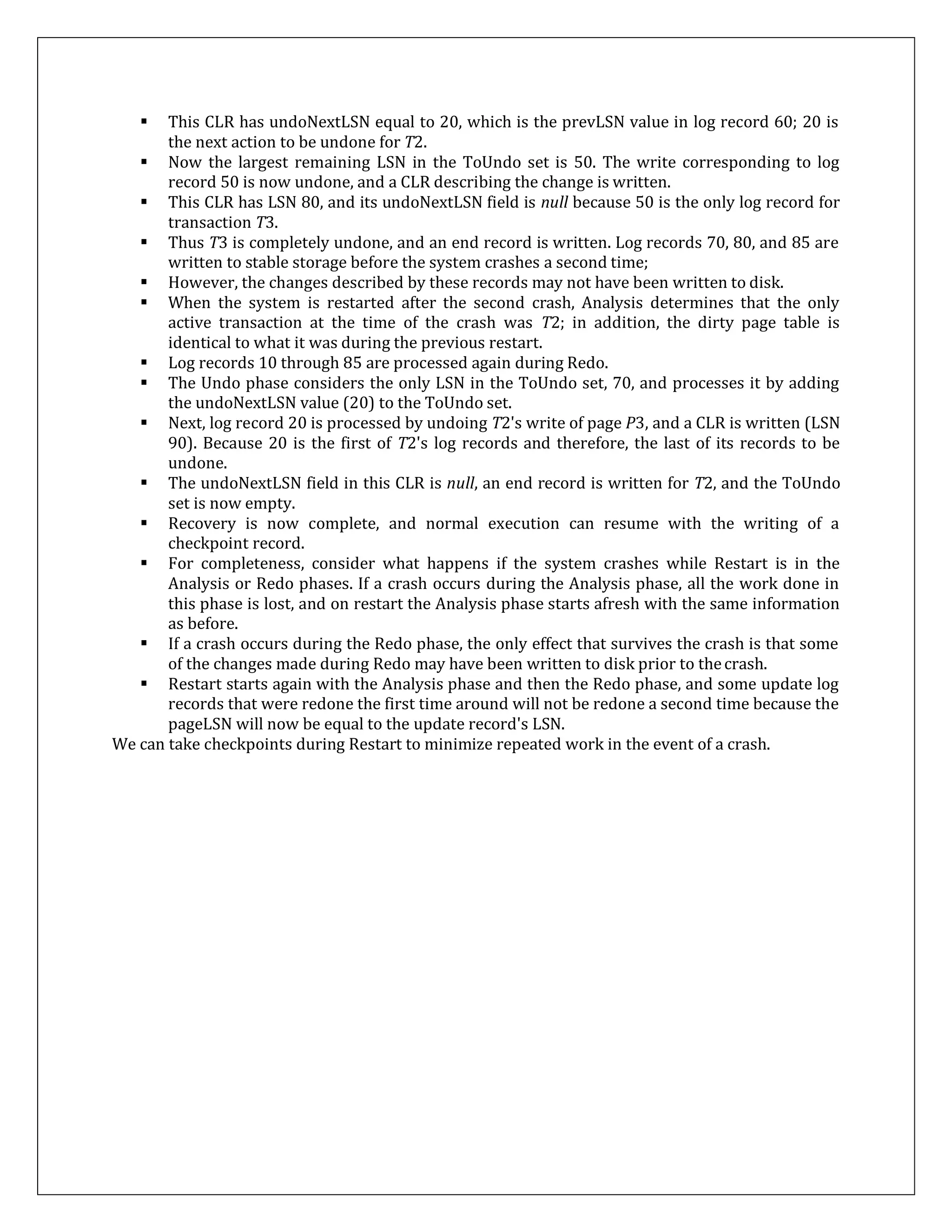
![ADDR2 VarChar2 50
CITY VarChar2 25
STATE VarChar2 25
PINCODE VarChar2 6
INSERT INTO ADDR_DTLS (ADDR_NO, CODE_NO, ADDR_TYPE, ADDR1, ADDR2, CITY, STATE,
PINCODE) VALUES(ADDR SEQ.NextVal, ‘B5’, ‘B’, ‘Vertex Plaza, Shop 4,’, ‘Western Express Highway,
Dahisar (East),’, ‘Mumbai’, ‘Maharashtra’, ‘400078’);
To reference the current value of a sequence:
SELECT < SequenceNnme >. CurrVal FROM DUAL;
Altering a Sequence
A sequence once created can be altered.
This is achieved by using the ALTER SEQUENCE statement.
Syntax:
ALTER SEQUENCE <SequenceName>
[INCREMENT BY <IntegerValue> MAXVALUE <IntegerValue> / NOMAXVALUE
MINVALUE <IntegerValue> / NOMINVALUE CYCLE / NOCYCLE
CACHE < IntegerVnlue >/ NOCACHE ORDER / NOORDER]
Note
The START value of the sequence cannot be altered.
Example 23:
Change the Cache value of the sequence ADDR_SEQ to 30 and interval between two
numbers as 2.
ALTER SEQUENCE ADDR_SEQ INCREMENT BY 2 CACHE 30;
Dropping A Sequence
The DROP SEQUENCE command is used to remove the sequence from the database.
Syntax:
DROP SEQUENCE < SequenceName > ;](https://image.slidesharecdn.com/tybsc-csdbms2notes-170810043037/75/Tybsc-cs-dbms2-notes-42-2048.jpg)
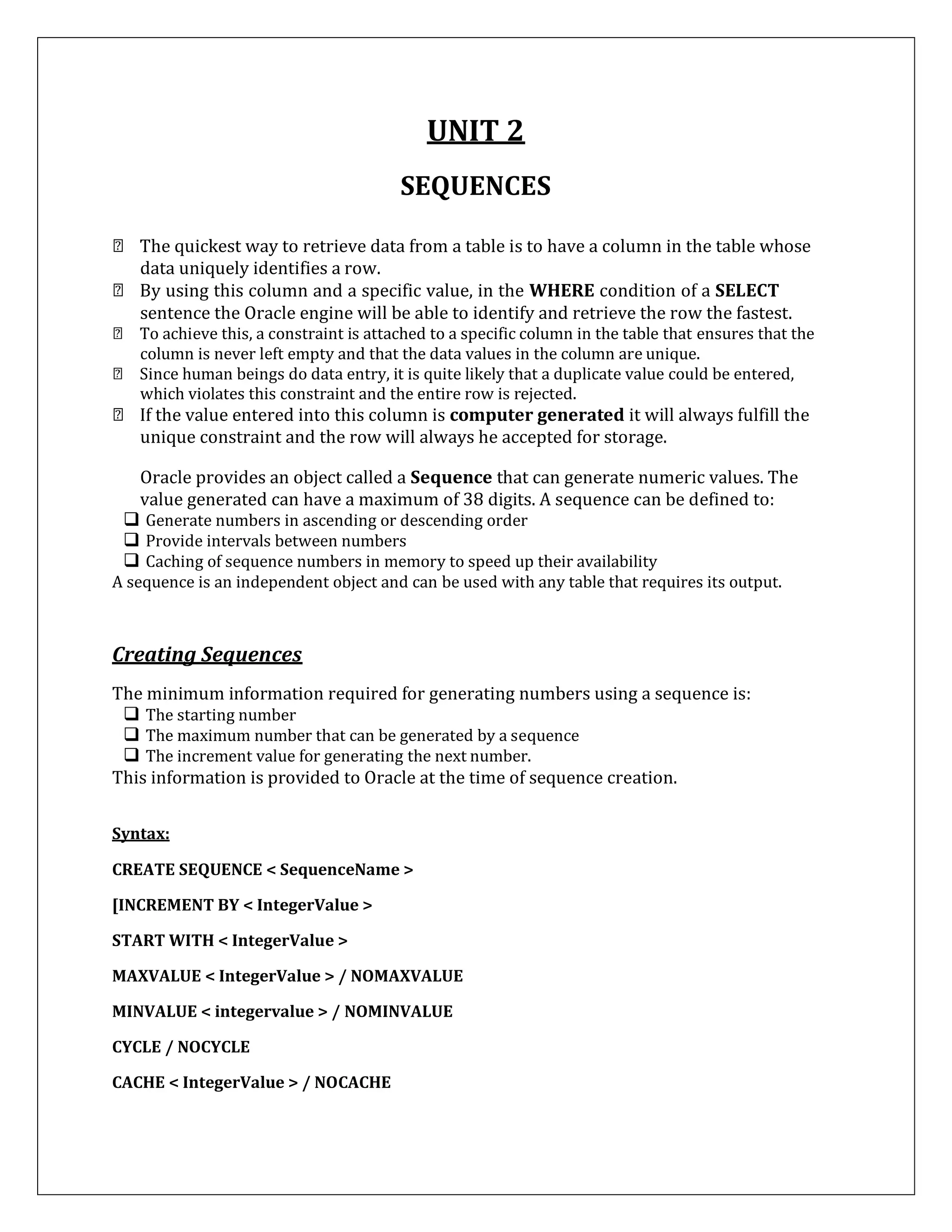
![ The call to the Oracle engine needs to be made only once to execute number ofstatements.
Oracle engine is called only once for each block, the speed of SQL statement execution is
vastly enhanced, when compared to the Oracle engine being called once for each SQL
statement.
Fundamentals of PL/SQL
The Character Set
Uppercase alphabets(A-Z)
Lowercase alphabets (a-z)
Numerals (0-9)
Symbols
( ) + - * / < > = ! ; : . ‘ @ % , “ # $ ^ & _ { } ? [ ]
Compound symbols used in PL/SQL block are
<> != -= ^= <= >= : = ** || << >>
Literals
Literal is a numeric value or a character string used to represent itself.
Numeric Literal
These can be either integer or floats. If a floats being represented, then the integer part
must be separated from float part by a period.
Example
25, 6.34, -5, 25e-03, .1
Logical (Boolean) Literal
These are predetermined constants. The values that can be assigned to this type are:
TRUE, FALSE, NULL
String Literal
These are represented by one or more legal characters and must be enclosed within
single quotes. The single quote character can be represented, by writing it twice in a
string literal.
Example](https://image.slidesharecdn.com/tybsc-csdbms2notes-170810043037/75/Tybsc-cs-dbms2-notes-46-2048.jpg)
![ ‘Hello world’
‘Don’t go without saving your work’
Character Literal
These are string literals consisting of single characters.
Example
‘*’
‘A’
PL/SQL Datatypes
Predefined Datatypes
Number Types
Character Types
National Character Types
Boolean Types
LOB Types
Date and Interval Types
Number Types
Number types let you store numeric data (integers, real numbers, and floating-point
numbers)
BINARY_INTEGER
We use the BINARY_INTEGER datatype to store signed integers.
BINARY_INTEGER values require less storage than NUMBER values.
BINARY_INTEGER Subtypes
NATURAL - Restrict an integer variable to non-negative or positive values
NATURALN - Prevent the assigning of nulls to an integer variable.
POSITIVE - Restrict an integer variable to non-negative or positive values
POSITIVEN - Prevent the assigning of nulls to an integer variable.
SIGNTYPE - Lets you restrict an integer variable to the values -1, 0, and 1.
NUMBER
We use the NUMBER datatype to store fixed-point or floating-point numbers.
We can specify precision, which is the total number of digits, and scale, which isthe
number of digits to the right of the decimal point. The syntax follows:
NUMBER[(precision,scale)]
To declare fixed-point numbers, for which you must specify scale, use the following
form:
NUMBER(precision,scale)
NUMBER Subtypes
DEC
DECIMAL
NUMERIC
INTEGER
INT](https://image.slidesharecdn.com/tybsc-csdbms2notes-170810043037/75/Tybsc-cs-dbms2-notes-47-2048.jpg)
![ SMALLINT
DOUBLE PRECISION
FLOAT
REAL
Use the subtypes DEC, DECIMAL, and NUMERIC to declare fixed-point numbers with a
maximum precision of 38 decimal digits.
Use the subtypes DOUBLE PRECISION and FLOAT to declare floating-point numbers with a
maximum precision of 126 binary digits, which is roughly equivalent to 38 decimal
digits.
REAL to declare floating-point numbers with a maximum precision of 63 binary digits,
this is roughly equivalent to 18 decimal digits.
Use the subtypes INTEGER, INT, and SMALLINT to declare integers with a maximum
precision of 38 decimal digits.
PLS_INTEGER
You use the PLS_INTEGER datatype to store signed integers
PLS_INTEGER values require less storage than NUMBER values. Also,PLS_INTEGER
operations use machine arithmetic, so they are faster than NUMBER and
BINARY_INTEGER operations.
Character Types
Character types let you store alphanumeric data, represent words and text, and manipulate
character strings.
CHAR
We use the CHAR datatype to store fixed-length character data. How the datais
represented internally depends on the database character set.
Maximum size up to 32767 bytes.
We can specify the size in terms of bytes or characters, where each character contains
one or more bytes, depending on the character set encoding.
CHAR[(maximum_size [CHAR | BYTE] )]
If you do not specify a maximum size, it defaults to 1.
VARCHAR2
You use the VARCHAR2 datatype to store variable-length character data.
VARCHAR2(maximum_size [CHAR | BYTE])](https://image.slidesharecdn.com/tybsc-csdbms2notes-170810043037/75/Tybsc-cs-dbms2-notes-48-2048.jpg)
![ National Character Types
The widely used one-byte ASCII and EBCDIC character sets are adequate to represent the
Roman alphabet, but some Asian languages, such as Japanese, contain thousands of
characters.
These languages require two or three bytes to represent each character.
NCHAR
You use the NCHAR datatype to store fixed-length (blank-padded if necessary) national
character data
The NCHAR datatype takes an optional parameter that lets you specify a maximumsize
in characters. The syntax follows:
NCHAR[(maximum_size)]
NVARCHAR2
You use the NVARCHAR2 datatype to store variable-length Unicode character data.
The NVARCHAR2 datatype takes a required parameter that specifies a maximum sizein
characters. The syntax follows:
NVARCHAR2(maximum_size)
Boolean Type
BOOLEAN
You use the BOOLEAN datatype to store the logical values TRUE, FALSE, and NULL.
Only logic operations are allowed on BOOLEAN variables.
The BOOLEAN datatype takes no parameters.
LOB Types
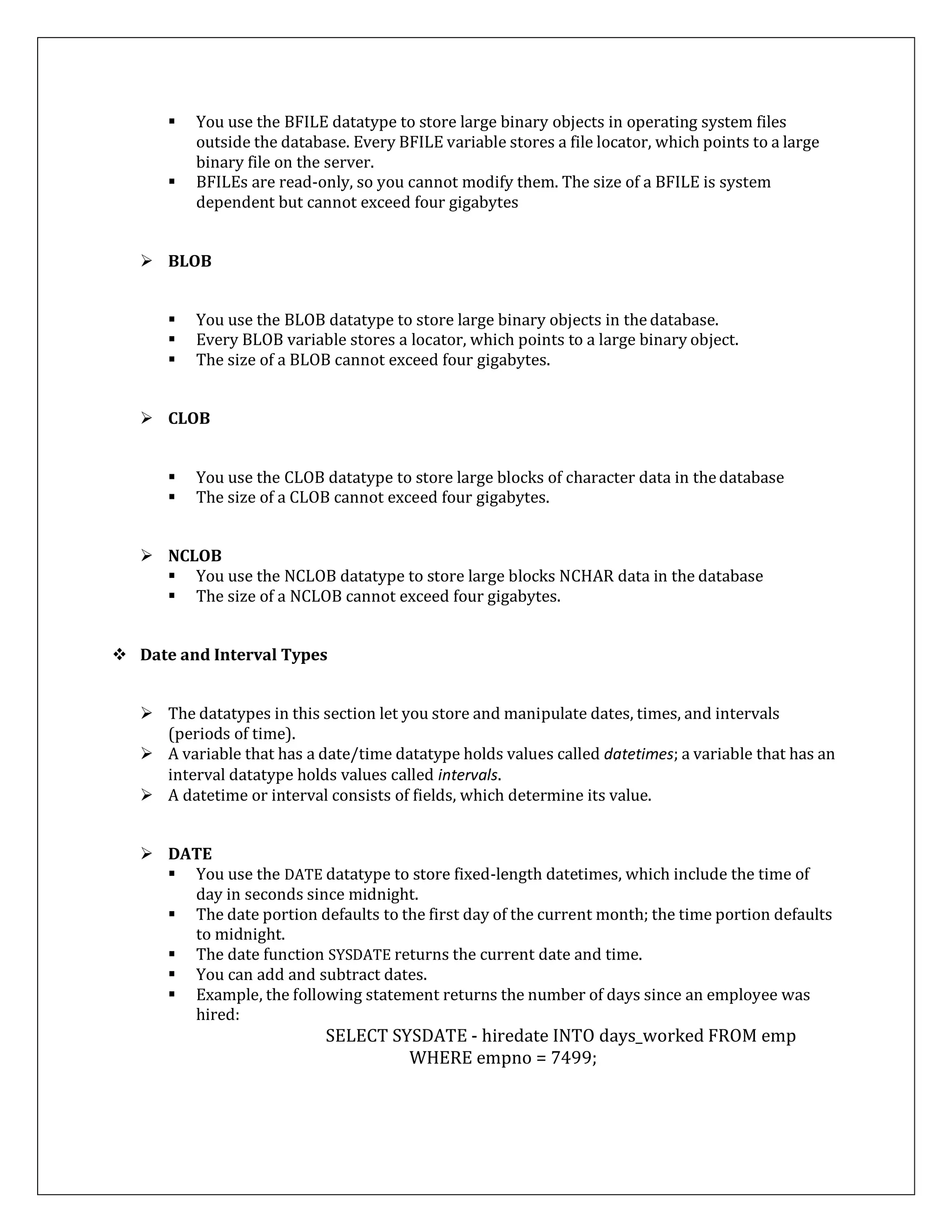
The LOB (large object) datatypes BFILE, BLOB, CLOB, and NCLOB let you store blocks of
unstructured data (such as text, graphic images, video clips, and sound waveforms) up to
four gigabytes in size.
PL/SQL operates on LOBs through the locators.
BFILE](https://image.slidesharecdn.com/tybsc-csdbms2notes-170810043037/75/Tybsc-cs-dbms2-notes-49-2048.jpg)
![ INTERVAL YEAR TO MONTH
You use the datatype INTERVAL YEAR TO MONTH to store and manipulate intervals of
years and months.
Example,
INTERVAL YEAR[(precision)] TO MONTH
where precision specifies the number of digits in the years field. You cannot
use a symbolic constant or variable to specify the precision; you must use an integer
literal in the range 0 .. 4. The default is 2.
INTERVAL DAY TO SECOND
You use the datatype INTERVAL DAY TO SECOND to store and manipulate intervals
of days, hours, minutes, and seconds.
The syntax is:
INTERVAL DAY[(leading_precision)] TO
SECOND[(fractional_seconds_precision)]
where leading_precision and fractional_seconds_precision specify the number of digits
in the days field and seconds field, respectively. In both cases, you cannot use a
symbolic constant or variable to specify the precision; you must use an integer
literal in the range 0 .. 9. The defaults are 2 and 6, respectively.
VARIABLES
Variables may be used to store the result of a query or calculations. Variables must be
declared before being used.
Variable Name
A variable name must begin with a character.
Variable length is 30 Characters.
Reserved words can not be used as variable names unless enclosed within the double
quotes.
Variables must be separated from each other by at least one space or by a punctuation
mark.
The case (upper/lower) is insignificant when declaring variable names.
Space can not be used in variable name.
Declaring variables](https://image.slidesharecdn.com/tybsc-csdbms2notes-170810043037/75/Tybsc-cs-dbms2-notes-51-2048.jpg)
![ We can declare a variable of any data type either native to the ORACLE or native to
PL/SQL.
Variables are declared in the DECLARE section of the PL/SQL block.
. Declaration involves the name of the variable followed by its data type followed by
semicolon (;).
To assign a value to the variable the assignment operator (:=) is used.
Syntax:
<Variable name> <type> [ :=<value> ];
Example:
Ename CHAR(10);
Assigning value to a variable
There are two ways to assign a value to a variable.
Using the assignment operator ( := )
Ex: sal := 1000.00;
Total_sal := sal – tax;
Selecting or fetching table data values in to variables.
Ex: SELECT sal INTO pay
FROM Employee WHERE emp_id = ‘E001’;
CONSTANT
A variable can be modified, a constant cannot.
Declaring Constant
Declaring a constant is similar to declaring a variable except that you have toadd
the key word CONSTANT and immediately assign a value toit.
Syntax:
<variable_name> CONSTANT <datatype> := <value>;
Example:
Pi CONSTANT NUMBER(3,2) := 3.14;
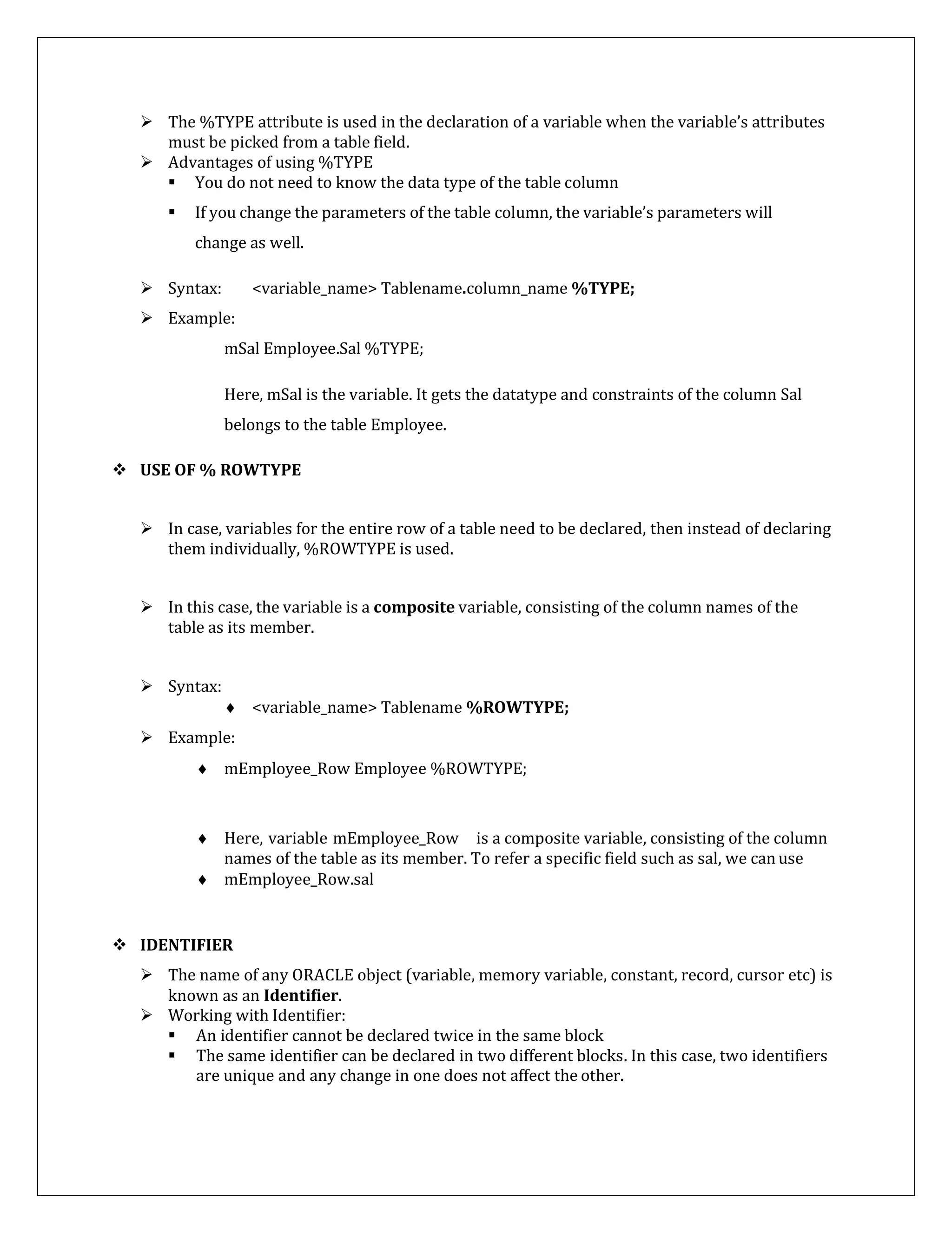
USE OF %TYPE
While creating a table user attaches certain attributes like data type and constraints.
These attributes can be passed on to the variables being created in PL/SQL using %TYPE
attribute.
This simplifies the declaration of variables and constants.](https://image.slidesharecdn.com/tybsc-csdbms2notes-170810043037/75/Tybsc-cs-dbms2-notes-52-2048.jpg)
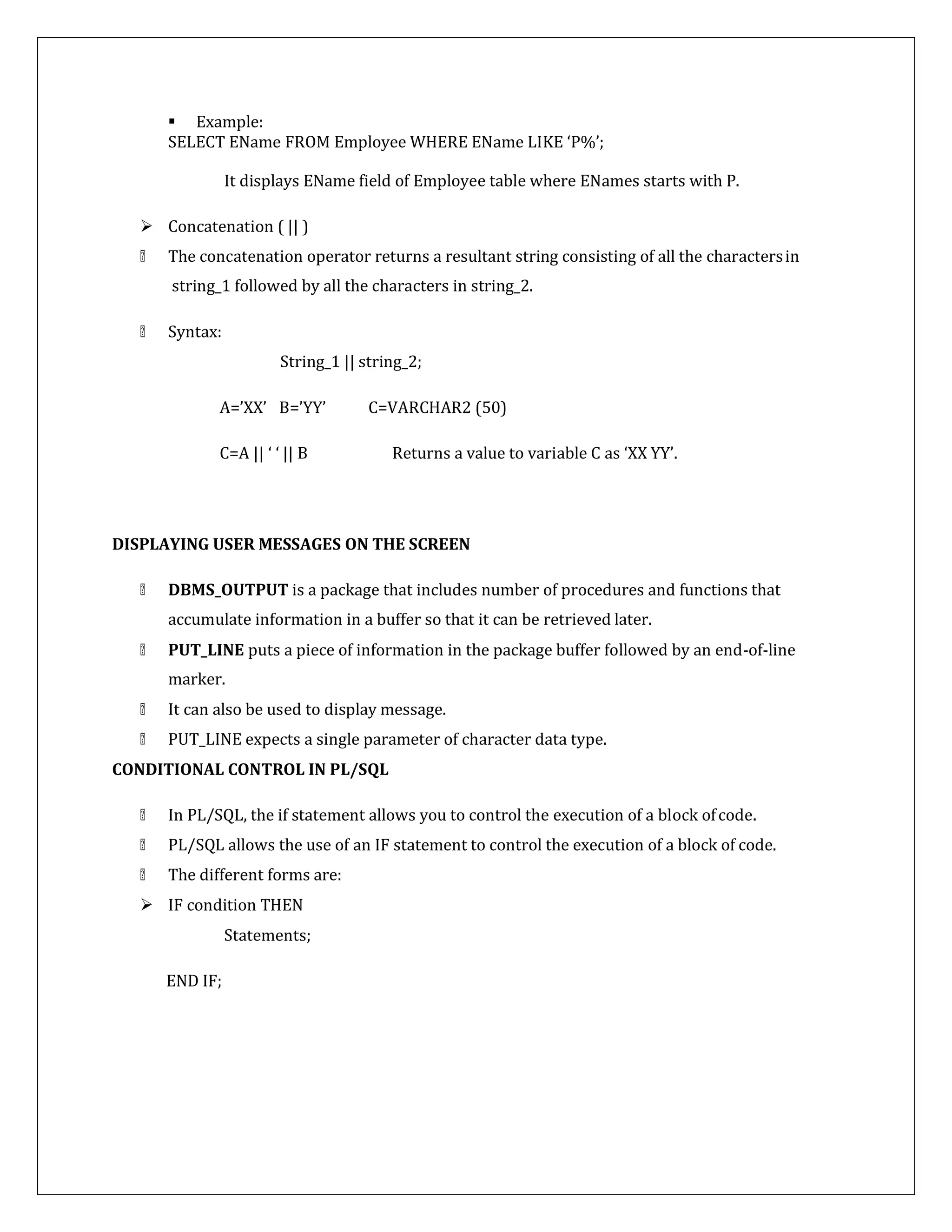
![LIKE OPERATOR
LIKE Operator is a Pattern matching operator.
It is used to compare a character string against a pattern.
Wild card characters:
o Percentage sign (%) - It matches any number of characters in a string.
o Underscore ( _ ) - It matches exactly one character.
Example:
SELECT EName FROM Employee WHERE EName LIKE ‘P%’;
It displays EName field of Employee table where ENames starts with P.
IN OPERATOR
It checks to see if a value lies within a specified list of values.
IN operator returns a BOOLEAN result, either TRUE or FALSE.
Syntax:
The_value [NOT] IN (value1, value2, value3……)
Example:
3 IN (4, 8, 7, 5, 3, 2) Returns TRUE
BETWEEN
It checks to see if a value lies within a specified range of value.
Low_End and Upper_Ends are inclusive.
Syntax:
the_value [NOT] BETWEEN low_end AND high_end.
Example:
5 BETWEEN –5 AND 10. Returns TRUE
IS NULL
It checks to see if a value is NULL.
Syntax:
Example:
the_value IS [NOT] NULL
IF balance IS NULL THEN](https://image.slidesharecdn.com/tybsc-csdbms2notes-170810043037/75/Tybsc-cs-dbms2-notes-55-2048.jpg)

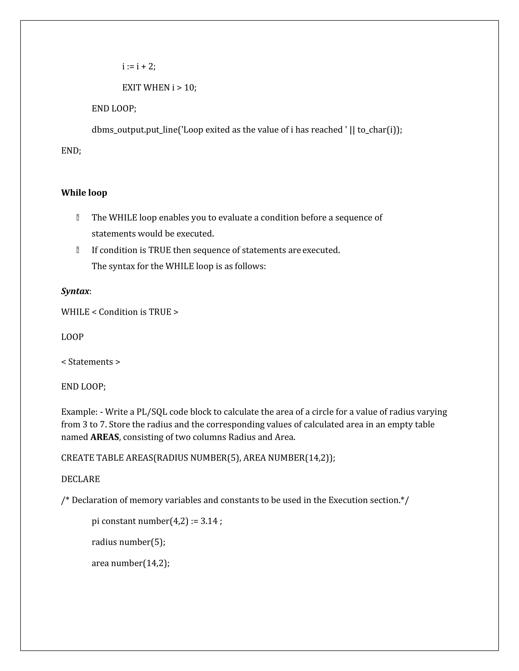
![BEGIN
/* Initialize the radius to 3, since calculations are required for radius 3 to 7 */
radius := 3;
/* Set a loop so that it fires till the radius value reaches 7 */
WHILE RADIUS <= 7
LOOP
/* Area calculation for a circle */
area := pi * power(radius,2);
/* Insert the value for the radius and its corresponding area calculated in the table */
INSERT INTO areas VALUES (radius, area);
END;
/* Increment the value of the variable radius by 1 */
radius := radius + 1;
END LOOP;
FOR LOOP
The FOR LOOP enables you to execute a loop for predetermined number of times.
The variable in the FOR loop need not be declared.
The increament value can not be specified.
The for loop variable is always incremented by 1.
Reverse is an optional keyword. If we specify keyword reverse then variable
considers last value first and then decrement it to get the start value.
The syntax for FOR LOOP is as follows:
FOR var IN [REVERSE] start…end
LOOP
Statements;
END LOOP;](https://image.slidesharecdn.com/tybsc-csdbms2notes-170810043037/75/Tybsc-cs-dbms2-notes-62-2048.jpg)
![END IF;
CASE Expression
A CASE expression selects a result from one or more alternatives, and returnsthe
result.
The CASE expression uses a selector, an expression whose value determineswhich
alternative to return.
A CASE expression has the following form:
CASE selector
WHEN expression1 THEN result1
WHEN expression2 THEN result2
...
WHEN expressionN THEN resultN
[ELSE resultN+1]
END;
The selector is followed by one or more WHEN clauses, which are checked
sequentially.
The value of the selector determines which clause is executed.
The first WHEN clause that matches the value of the selector determines the result
value, and subsequent WHEN clauses are not evaluated.
An example follows:
DECLARE
grade CHAR(1) := 'B';
appraisal VARCHAR2(20);
BEGIN
appraisal :=
CASE grade
WHEN 'A' THEN 'Excellent'
WHEN 'B' THEN 'Very Good'
WHEN 'C' THEN 'Good'
WHEN 'D' THEN 'Fair'
WHEN 'F' THEN 'Poor'
ELSE 'No such grade'
END;
END;
The optional ELSE clause works similarly to the ELSE clause in an IF statement.
If the value of the selector is not one of the choices covered by a WHEN clause, the
ELSE clause is executed.](https://image.slidesharecdn.com/tybsc-csdbms2notes-170810043037/75/Tybsc-cs-dbms2-notes-66-2048.jpg)
![If no ELSE clause is provided and none of the WHEN clauses are matched, the
expression returns NULL.
Searched CASE Expression
PL/SQL also provides a searched CASE expression, which has the form:
CASE
WHEN search_condition1 THEN result1
WHEN search_condition2 THEN result2
...
WHEN search_conditionN THEN resultN
[ELSE resultN+1]
END;
A searched CASE expression has no selector.
Each WHEN clause contains a search condition that yields a Boolean value, which lets
you test different variables or multiple conditions in a single WHEN clause.
An example follows:
DECLARE
grade CHAR(1);
appraisal VARCHAR2(20);
BEGIN
...
appraisal :=
CASE
WHEN grade = 'A' THEN 'Excellent'
WHEN grade = 'B' THEN 'Very Good'
WHEN grade = 'C' THEN 'Good'
WHEN grade = 'D' THEN 'Fair'
WHEN grade = 'F' THEN 'Poor'
ELSE 'No such grade'
END;
...
END;
The search conditions are evaluated sequentially.
The Boolean value of each search condition determines which WHEN clause is
executed.
If a search condition yields TRUE, its WHEN clause is executed.
After any WHEN clause is executed, subsequent search conditions are not evaluated.
If none of the search conditions yields TRUE, the optional ELSE clause is executed.](https://image.slidesharecdn.com/tybsc-csdbms2notes-170810043037/75/Tybsc-cs-dbms2-notes-67-2048.jpg)
![CASE
WHEN search_condition1 THEN sequence_of_statements1;
WHEN search_condition2 THEN sequence_of_statements2;
...
WHEN search_conditionN THEN sequence_of_statementsN;
[ELSE sequence_of_statementsN+1;]
END CASE;
The searched CASE statement has no selector.
Its WHEN clauses contain search conditions that yield a Boolean value,not
expressions that can yield a value of any type.
The search conditions are evaluated sequentially.
The Boolean value of each search condition determines which WHEN clause is
executed.
If a search condition yields TRUE, its WHEN clause is executed. If any WHEN clause
is executed, control passes to the next statement, so subsequent search conditions
are not evaluated.
If none of the search conditions yields TRUE, the ELSE clause is executed. The ELSE
clause is optional. However, if you omit the ELSE clause, PL/SQL adds the following
implicit ELSE clause:
An example follows:
CASE
WHEN grade = 'A' THEN dbms_output.put_line('Excellent');
WHEN grade = 'B' THEN dbms_output.put_line('Very Good');
WHEN grade = 'C' THEN dbms_output.put_line('Good');
WHEN grade = 'D' THEN dbms_output.put_line('Fair');
WHEN grade = 'F' THEN dbms_output.put_line('Poor');
ELSE dbms_output.put_line('No such grade');
END CASE;
Handling Null Values in Comparisons and Conditional Statements
When working with nulls, you can avoid some common mistakes by keeping in mind the following
rules:
Comparisons involving nulls always yield NULL
Applying the logical operator NOT to a null yields NULL
In conditional control statements, if the condition yields NULL, its associated sequence of
statements is not executed
If the expression in a simple CASE statement or CASE expression yields NULL, it cannot be
matched by using WHEN NULL. In this case, you would need to use the searched case syntax
and test WHEN expression IS NULL.](https://image.slidesharecdn.com/tybsc-csdbms2notes-170810043037/75/Tybsc-cs-dbms2-notes-69-2048.jpg)
![ORACLE TRANSACTIONS
PL / SQL TRANSACTIONS
A series of one or more SQL statements that are logically related or a series of operations
performed on Oracle table data is termed as a Transaction.
Oracle treats this logical unit as a single entity.
Oracle treats changes to table data as a two-step process. First, the changes requested are
done.
To make these changes permanent a COMMIT statement has to be given at the SQL
prompt.
A ROLLBACK statement given at the SQL prompt can be used to undo a part of or the entire
transaction.
Specifically, a transaction is a group of events that occur between any of the following
events:
Connecting to Oracle
Disconnecting from Oracle
Committing changes to the database table
Rollback
Closing Transactions
A transaction can be closed by using either a commit or a rollback
statement.
By using these statements. table data can be changed or all the changes made
to the table data undone.
Using COMMIT:
A COMMIT ends the current transaction and makes permanent any changes made
during the transaction.
All transactional locks acquired on tables are released.
Syntax:
COMMIT;
Using ROLLBACK:
A ROLLBACK does exactly the opposite of COMMIT.
It ends the transaction but undoes any changes made during the transaction.
All transactional locks acquired on tables are released.
Syntax:
ROLLBACK [WORK] [TO [SAVEPOINT] <SavePointName>];
where,
WORK Is optional and is provided for ANSI compatibility](https://image.slidesharecdn.com/tybsc-csdbms2notes-170810043037/75/Tybsc-cs-dbms2-notes-71-2048.jpg)
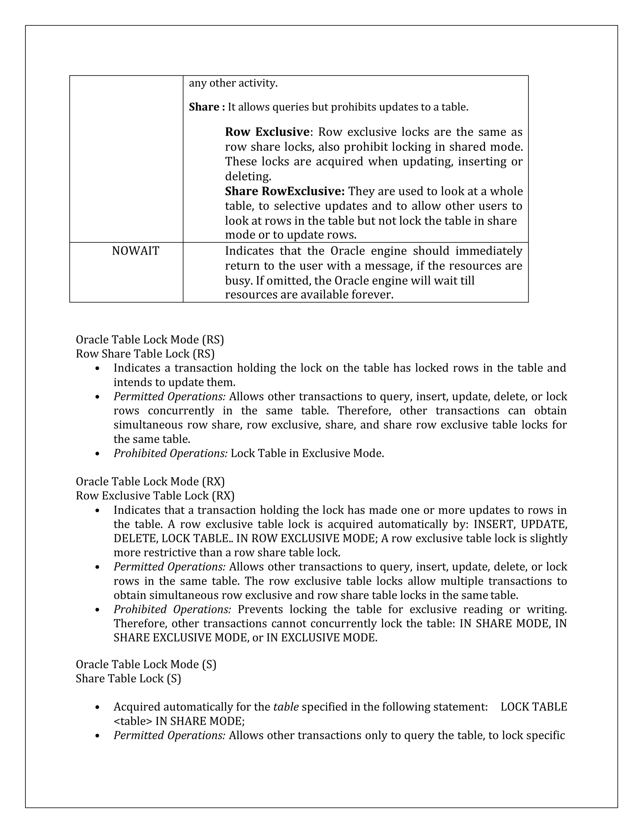
![SELECT … FOR UPDATE with NOWAIT Option
In order to avoid unnecessary waiting time, a NOWAIT option can be used to inform the Oracle
engine to terminate the SQL statement if the record has already been locked. If this happens the
Oracle engine terminates the running DML and comes up with a message indicating that the
resource is busy.
If Client B fires the following select statement now with a NOWAIT clause:
Client B> SELECT * FROM ACCT_MSTR WHERE ACCT_NO ='SB9' FOR UPDATE NOWAIT;
Output:
Since Client A has already locked the record SB9 when Client B tries to acquire a shared
lock on the same record the Oracle Engine displays the following message:
SQL> 00054: resource busy and acquire with nowait specified.
The SELECT ... FOR UPDATE cannot be used with the following:
Distinct and the Group by clause
Set operators and Group functions
Using Lock Table Statement
To manually override Oracle's default locking strategy by creating a data lock in a specific
mode.
Syntax:
LOCK TABLE <TabIeName> [, <TabIeName>] ...
IN {ROW SHARE|ROW EXCLUSIVEISHARE UPDATE|
SHAREISHARE ROW EXCLUSIVE I EXCLUSIVE }
[NOWAIT]
where,
TableName Indicates the name of table(s), view(s) to be locked. In
case of views, the lock is placed on underlying tables.
IN Decides what other locks on the same resource can
exist simultaneously. For example, if there is an
exclusive lock on the table no user can update rows in
the table. It can have any of the following values:
Exclusive: They allow query on the locked resource but prohibit](https://image.slidesharecdn.com/tybsc-csdbms2notes-170810043037/75/Tybsc-cs-dbms2-notes-79-2048.jpg)
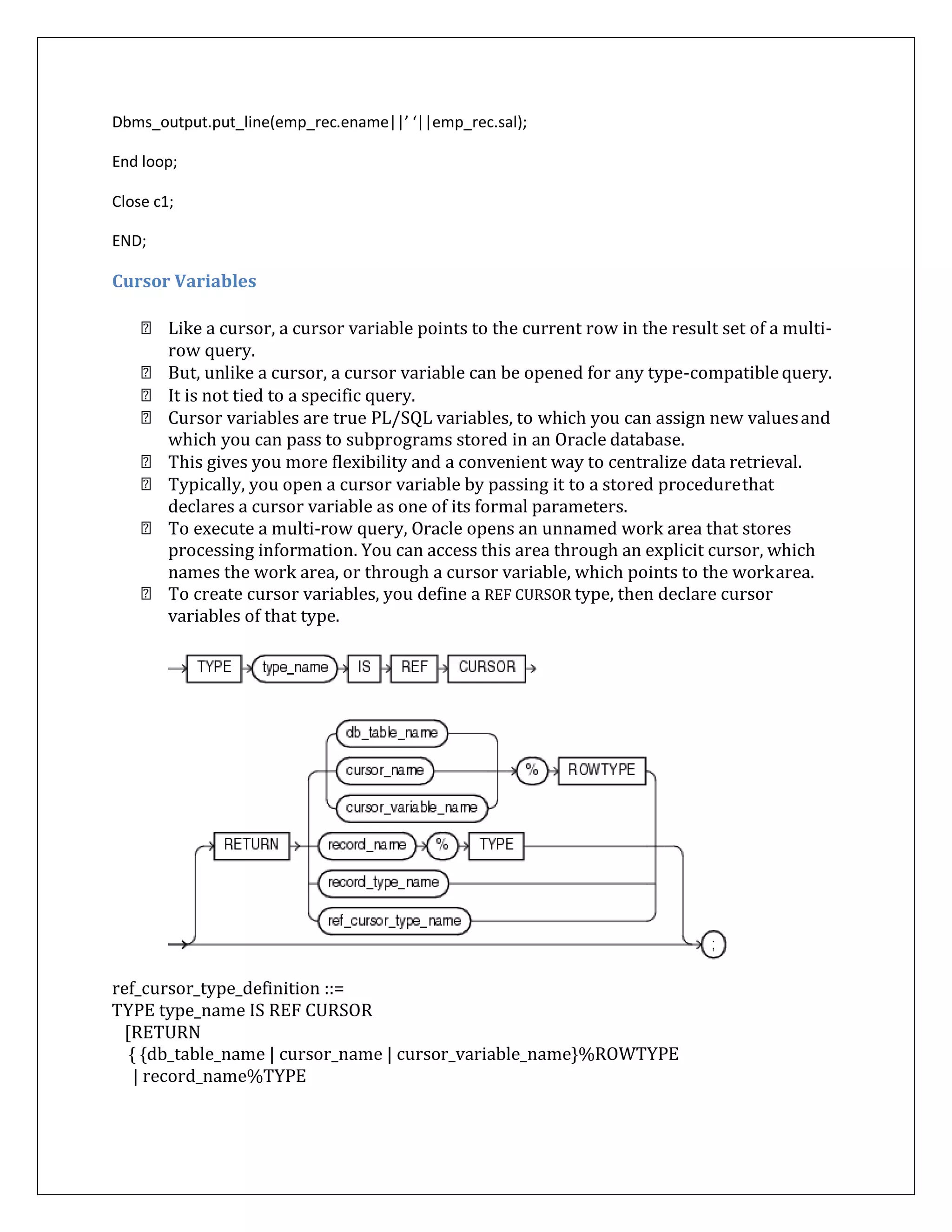
![| record_type_name
| ref_cursor_type_name
}];
ref_cursor_variable_declaration ::=
cursor_variable_name type_name;
Keyword and Parameter Description
cursor_name
o An explicit cursor previously declared within the current scope.
cursor_variable_name
o A PL/SQL cursor variable previously declared within the current scope.
db_table_name
o A database table or view, which must be accessible when the declaration is
elaborated.
record_name
o A user-defined record previously declared within the current scope.
record_type_name
o A user-defined record type that was defined using the datatype specifier RECORD.
REF CURSOR
o Cursor variables all have the datatype REF CURSOR.
RETURN
o Specifies the datatype of a cursor variable return value. You can use the %ROWTYPE
attribute in the RETURN clause to provide a record type that represents a row in a
database table, or a row from a cursor or strongly typed cursor variable. You can use
the %TYPE attribute to provide the datatype of a previously declared record.
Types of Cursor Variables
REF CURSOR types can be strong (with a return type) or weak (with no return type).
Strong REF CURSOR types are less error prone because the PL/SQL compiler lets you
associate a strongly typed cursor variable only with queries that return the right set of
columns.
Weak REF CURSOR types are more flexible because the compiler lets you associate a weakly
typed cursor variable with any query.
Because there is no type checking with a weak REF CURSOR, all such types are
interchangeable. Instead of creating a new type, you can use the predefinedtype
SYS_REFCURSOR.
The following procedure opens the cursor variable generic_cv for the chosen query:
PROCEDURE open_cv (generic_cv IN OUT GenericCurTyp,choice NUMBER) IS
BEGIN](https://image.slidesharecdn.com/tybsc-csdbms2notes-170810043037/75/Tybsc-cs-dbms2-notes-94-2048.jpg)
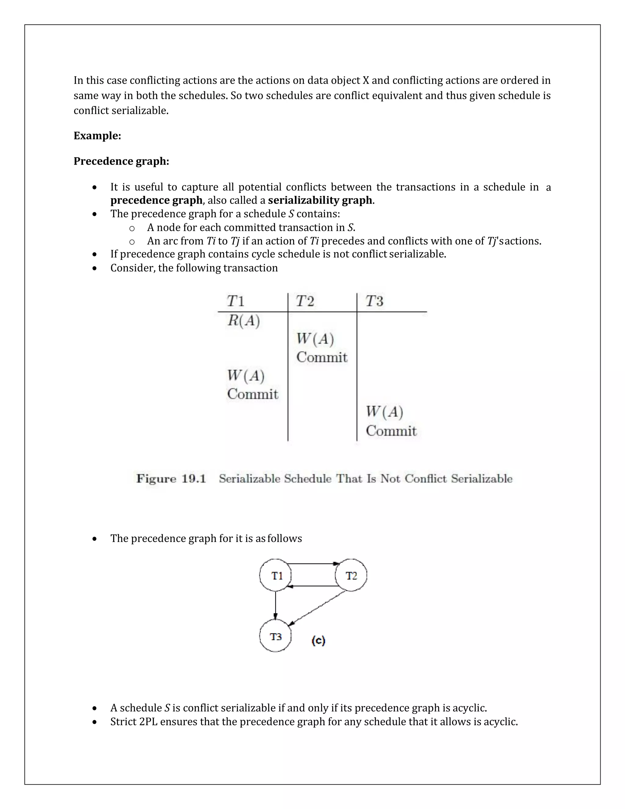
![The process of decomposition of a relation R into a set of relations R1, R2....Rn is based on
identifying attributes and using that as a basis of decomposition.
R=R1 U R2 U………Rn.
This is a process of dividing one table into multiple tables using projection operator.
We may decompose tables into vertical segments. Vertical fragmentation is done with help of
projection operator. By taking projection of original table we can create multiple vertically
fragmented tables.
Original table
Decomposition
Q.] Explain decomposition?
If a relation is not in the normal form and we wish the relation to be normalized so that some of
the anomalies (like insert, update or delete anomalies) can be eliminated, it is necessary to
decompose the relation in two or more relations.
Eno Ename Class
1 Mahesh BE
2 Yogesh SE
3 Amit TE
Vertically Decomposed
Tables
Eno Ename
1 Mahesh
2 Yogesh
3 Amit
Eno Class
1 BE
2 SE
3 TE](https://image.slidesharecdn.com/tybsc-csdbms2notes-170810043037/75/Tybsc-cs-dbms2-notes-100-2048.jpg)
![Q.] Explain the desirable Properties of decomposition:
The main properties of decomposition are as listed below,
a. Lossless-join decomposition
b. Dependency preservation
c. Lack of redundancy (Repetition of information)
1) Lossless join decomposition
It is clear that decomposition must be lossless so that we do not lose any information from the
relation that is decomposed. Lossless join decomposition ensures that we can never get the
situation where false tuple are generated in relation. For every value on the join attributes there
should be a unique tuple in one of the relations. For following table to become lossless we need
to go for following steps.
Deptjd Dname Stud_Id Sname Location
10 Development 1 Sushant Mahim
20 Teaching 2 Snehal Vashi
30 HR 3 Pratiksha Warli
20 Admin 4 Supraja Dadar
a.Let R1 and R2 form decomposition of relation R.
b.Decompose the relation schema Department-Student into
Department-schema = (Dept_Id, Dname)
Student-schema = (Stud_id, Sname, Location)
c. The attributes in common must be a key for one of the relation for decomposition to be
lossless. R1 ∩ R2 ≠ Φ. There must not be null.](https://image.slidesharecdn.com/tybsc-csdbms2notes-170810043037/75/Tybsc-cs-dbms2-notes-101-2048.jpg)
![3) Lack of Redundancy ( Repetition of information)
Decomposition that we have done should not suffer from any repetition of information problem.
For eg: STUDENT and SECTION data are separated into distinct relations. Thus we do not
have to repeat STUDENT data for each SECTION.
If a single SECTION is made into several STUDENTS, we do not have to repeat the SECTION
data for each STUDENT.
IT is desirable not to have any redundancy in database. This property may be achieved by
normalization process.
Q.] What is a Lossy- join decomposition?
We decomposed a relation intuitively but, still we need a better basis for deciding
decompositions since intuition may not always be correct. A careless decomposition may lead
to problems like loss of information.
Department-Student Schema = (Dept_Id, Dname, Stud_Id, Sname, Location)
Deptjd Dname Stud_Id Sname Location
10 Development 1 Sushant Mahim
20 Teaching 2 Snehal Vashi
30 HR 3 Pratiksha Warli
20 Admin 4 Supraja Dadar
Suppose we decompose the above relation into two relations Department and Student as
follows :](https://image.slidesharecdn.com/tybsc-csdbms2notes-170810043037/75/Tybsc-cs-dbms2-notes-103-2048.jpg)
![Schema 2: Student Schema contains (Stud_Id, Sname, Location)
All the information that was in the relation 'Department' appears to be still available in
'Department-Student' schema but this is not so. Suppose, we would need to join 'Department'
and 'Student' table this join becomes lossy join decomposition.
As R, n R2 = O
So, there is no column common between them, therefore joining not possible. A lossless
decomposition is that which guarantees that the join will result in exactly the same relation as
was decomposed
.
Q.] Explain Functional Dependency:
Schema 1: Department Schema containing (Deptjd, Dname)
Deptjd Dname
10 Development
20 Teaching
30 HR
Studjd Sname Location
1 Sushant Mahim
2 Snehal Vashi
3 Pratiksha Warli
4 Supraja Dadar
The concept of functional dependency is given by E. F. Codd which is also called as
normalization process. This concept is used to define various normal forms.](https://image.slidesharecdn.com/tybsc-csdbms2notes-170810043037/75/Tybsc-cs-dbms2-notes-104-2048.jpg)
![Functional dependency is a type of constraints exists between multiple attributes of a relation.
Functional Dependency (FD) determines the set of values or the attribute based on another
attribute
It is denoted by (—>)
This form can be written as Y is functionally dependent on X or X determines Y.
E code —> E Name
We can say column X is functionally dependent on other column Y. If data value in column X
change when data value in another column Y is modified.
an FD X Y essentially says that if two tuples agree on the values in attributes X, they must
also agree on the values in attributes Y.
Functional Dependency provides a formal mechanism to express constraints between various
attributes of a relation.
For Eg, let us say in below table if the name of employee is changed its ID also need to be
changed so, we can say NAME column is dependent on employee ID column, i.e. For different
name of employee different ID is given.
Employee Table
ID Name
• a • •
MahOOl Mahesh ....
Q.] Explain the Types of Functional Dependencies
1. Full Functional Dependency:
A Functional Dependency A —> B is a full functional dependency if removal of any attributes
from A means that the dependency does not hold any more.
Example](https://image.slidesharecdn.com/tybsc-csdbms2notes-170810043037/75/Tybsc-cs-dbms2-notes-105-2048.jpg)
![{Emp_no, Project_no} -> HOURS i.e. Emp_no —> Hours and Project_no —> Hours
In the above example, Hours is fully functionally dependent on both Emp_no and Project_no.
The number of hours spent on the project by a particular employee cannot be determined with
the project number (Project_no) alone. It needs the employee number (Emp_no) as well.
2. Partial Functional Dependency:
A partial dependency means that a non key column is depend on some columns in composite
primary key of a table. An FD A —> B is a partial dependency if there is some attribute X € A (X
subset of A), that can be removed from A and the dependency will still hold.
Example
{Emp_no, Project_no} —> Ename that is, Emp_no —> Ename
In the above example, Ename is partially dependent on {Emp_no, Project_no} since employee
name (ename) can be determined using the employee id (Emp_no) alone even if project_no is
removed from the relation.
Note: For a table to be in 2nd Normal form there should be no partial dependencies.
Q.] Explain Transitive Dependency
This concept is used when there is redundancy in database. If changing any non key column
(column other then key column) causes change in other non key column in such situations you
may have transitive dependency.
When one non key attribute is functionally dependent on another non key attribute then such a
dependency is called as transitive dependency.
Non Key Attribute —» Non Key Attribute
An FD X —>Y in a relation R is a transitive dependency, if there is a set of attributes Z that is
not a subset of any key of R, and both X —» Z and Z —> Y holds true.
For eg:
EMP_DEPT {Eno, Ename, Dnumber, DeptMgrNo}
Eno —> DeptmgrNo is transitive](https://image.slidesharecdn.com/tybsc-csdbms2notes-170810043037/75/Tybsc-cs-dbms2-notes-106-2048.jpg)
![Dependency of DeptMgrNo on key attribute Eno is transitive as DeptMgrNo depends on
Dnumber and DNumber itself is dependent on Eno.
Eno —> Dnumber and Dnumber —> DMgrNo
Q.] Armstrong's Axioms - Closures of Functional Dependency
Given that A, B and C are sets of attributes in a relation R; one can derive several properties of
functional dependencies.
Axioms are nothing but rules of inference which provides a simple technique for reasoning
about functional dependencies.
1) Primary Rules
a. Subset Property (Axiom of Reflexivity)
If Y is a subset of X, then X —» Y
b. Augmentation (Axiom of Augmentation)
If X —> Y, then XZ -> YZ
c. Transitivity (Axiom of Transitivity)
If X -> Y and Y -> Z, then X -> Z
2) Secondary Rules (Based on above rules)
a. Union: If X -» Y and X -> Z, then X -> YZ
b. Decomposition: If X —> YZ and X -> Y, then X -> Z
c. Pseudo Transitivity: If X —> Y and YZ -> W, then XZ -> W
Example : Consider relation R = (A,B,C,D,E,F) having set of FD's
A -> B A-> C](https://image.slidesharecdn.com/tybsc-csdbms2notes-170810043037/75/Tybsc-cs-dbms2-notes-107-2048.jpg)
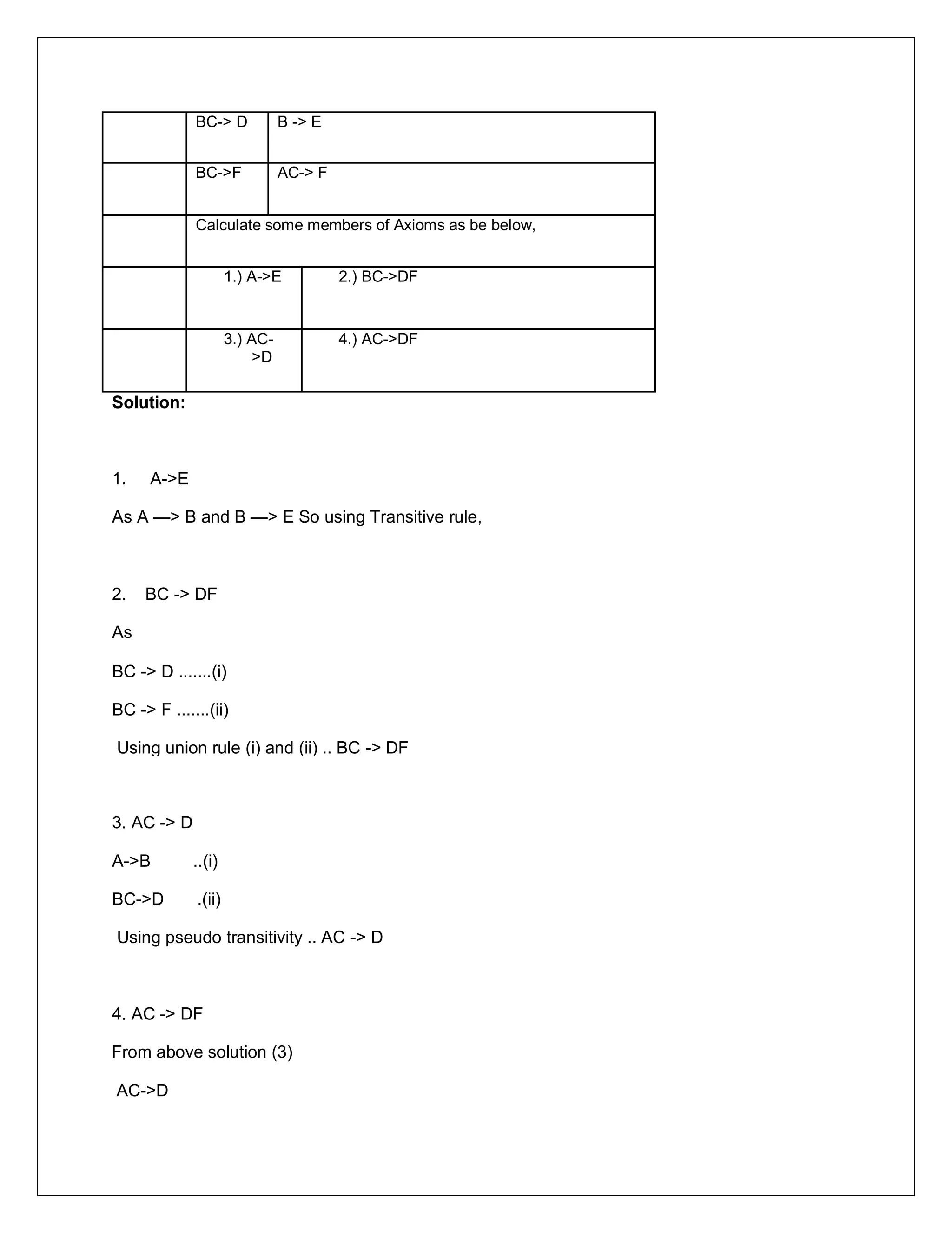
![AC->F
Therefore, AC->DF
Normalization
Normalization is a step by step decomposition of complex records into simple records.
Normalization results in tables that satisfy some constraints and are represented in a simple
manner. This process is also called as canonical synthesis. This is a relational database
design process to avoid data redundancy by applying some constraints on data to avoid various
data anomalies.
For E.g. If same information is repeated in multiple tables of database then there are chances
that these tables will not be consistent in case of data updation, insertion or deletion. This
instance may lead to problems of data integrity. A normalized table is less vulnerable to such
data anomalies.
Normalization is a process of designing a consistent database by minimizing redundancy
and ensuring data integrity through decomposition which is lossless.
Q.] Goals/ Importance of Database Normalization
1. Ensures Data Integrity
Data integrity ensures the correctness of data stored within the database. It is achieved by
imposing integrity constraints. An integrity constraint is a rule, which restricts values present in
the database.
There are three integrity constraints:
(i) Entity constraints: The entity integrity rule states that the value of the primary key can never
be a null value. Because a primary key is used to identify a unique row in a relational table, its
value must always be specified and should never be unknown.The integrity rule requires that
insert, update and delete operations maintain the uniqueness and existence of all primarykeys.](https://image.slidesharecdn.com/tybsc-csdbms2notes-170810043037/75/Tybsc-cs-dbms2-notes-109-2048.jpg)
![(ii) Domain Constraints: Only permissible values of an attribute are allowed in a relation.
(iii) Referential Integrity constraints: The referential integrity rule states that if a relational
table has a foreign key, then every value of the foreign key must either be null or match the
values in the relational table (referenced table) in which that foreign key is a primary key.
2.) Prevents Redundancy in data: A non-normalized database is vulnerable to data
anomalies, if it stores data redundantly. If data is stored in two locations, but the data is updated
in only one of the locations, then that data becomes inconsistent. A normalized database stores
non-primary key data in only one location.
3.) To avoid Data Anomaly: A non-normalized table can suffer from logical inconsistencies of
various types, and from data anomalies. A Relational database table should be designed in
such a way that it will avoid all data anomalies.
Q.] Which are the different anomalies related to normalization:-
1) Update anomaly: Same information can be present in multiple records of various relations;
updates to only one table may result in logical inconsistencies.
Example each record in an "Emp_Salary" table might contain an Emp_ID, Ename, Address,
Salary. Thus a change of address for a particular Employee will potentially need to be applied to
multiple tables such as Employee table. If all the records are not updated then some tables may
leave in an inconsistent state.
2) An insertion anomaly: There is a possibility in which certain facts cannot be recorded at all
or they are not yet recorded.
Example
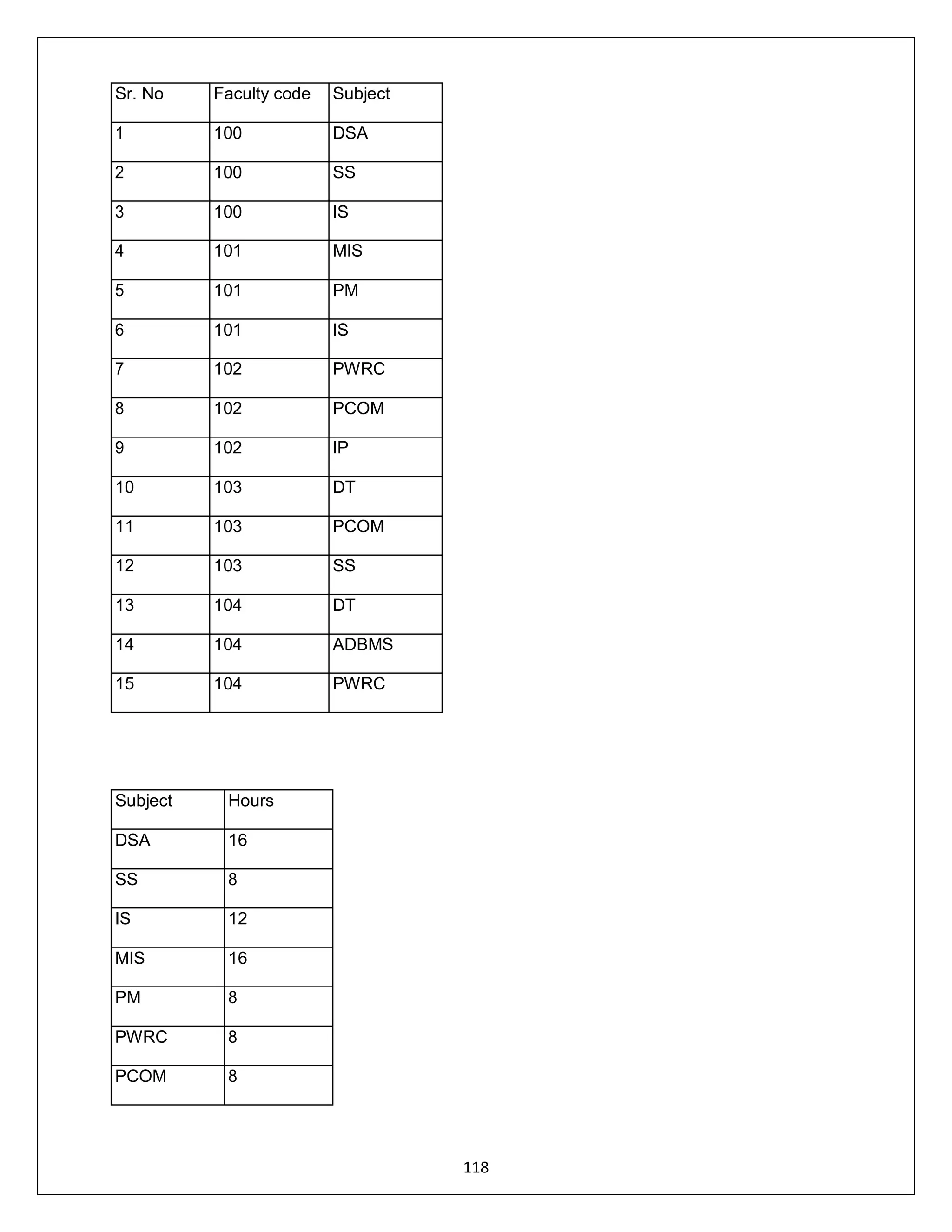
Consider a table, Faculty (Faculty_ID, FName, Subject_Code, Subject, Class). We can add the
details of any faculty member who teaches for a certain subject in a certain class, but we cannot
record the details of a new faculty member who has not yet been assigned to teach any subject
or class. So, subject and class column may be empty initially. If data deleted from one table all
relevant data must also be deleted or redundant.](https://image.slidesharecdn.com/tybsc-csdbms2notes-170810043037/75/Tybsc-cs-dbms2-notes-110-2048.jpg)
![110
3) Deletion Anomaly: If data deleted from one table all relevant data in another related tables
must also be deleted otherwise it will create redundancy problem. Deletion of some data from a
relation necessitates the deletion of some unrelated data also called as deletion anomaly.
Example
In the previous example, the table suffers from this type of anomaly. If a faculty member
temporarily ceases to be assigned a subject, we must delete the entire record on which that
faculty member appears.
Normal Forms
Forms are designed to logically address potential problems such as inconsistencies and
redundancy in information stored in the database. A database is said to be in one of the Normal
Forms, if it satisfies the rules required by that form as well as the previous form; it also will not
suffer from any of the problems addressed by the form.
Q.] State and explain Types of Normal Forms
a. First normal form (INF)
b. Second normal form (2NF)
c. Third normal form (3NF)
d. Boyce-Codd normal form (BCNF)
e. Fourth normal form (4NF)
f. Fifth Normal Form (5NF)
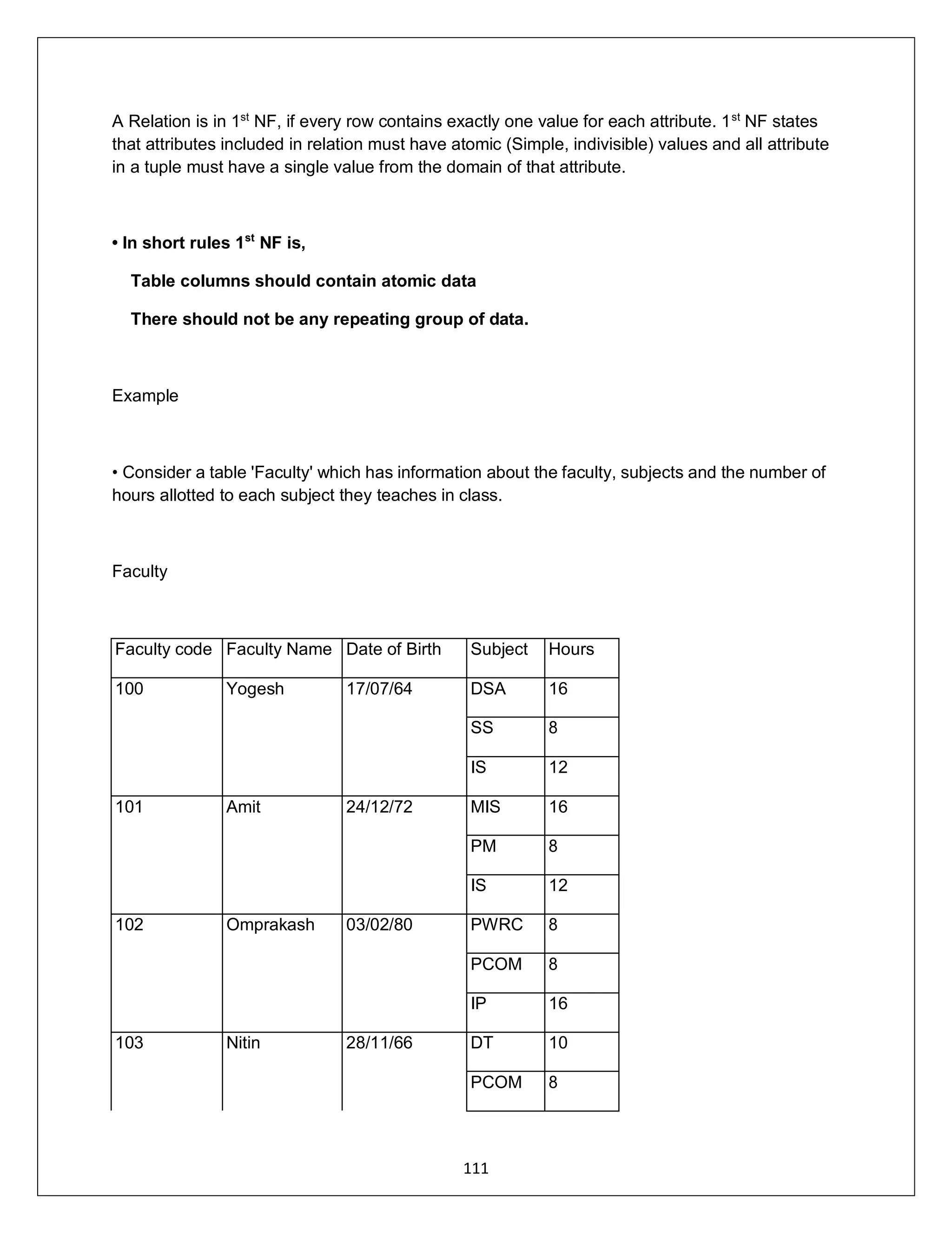
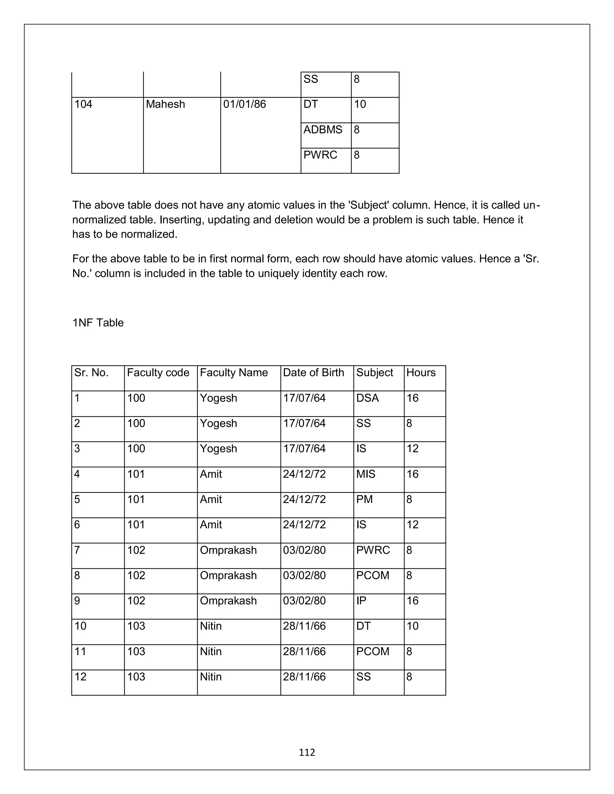
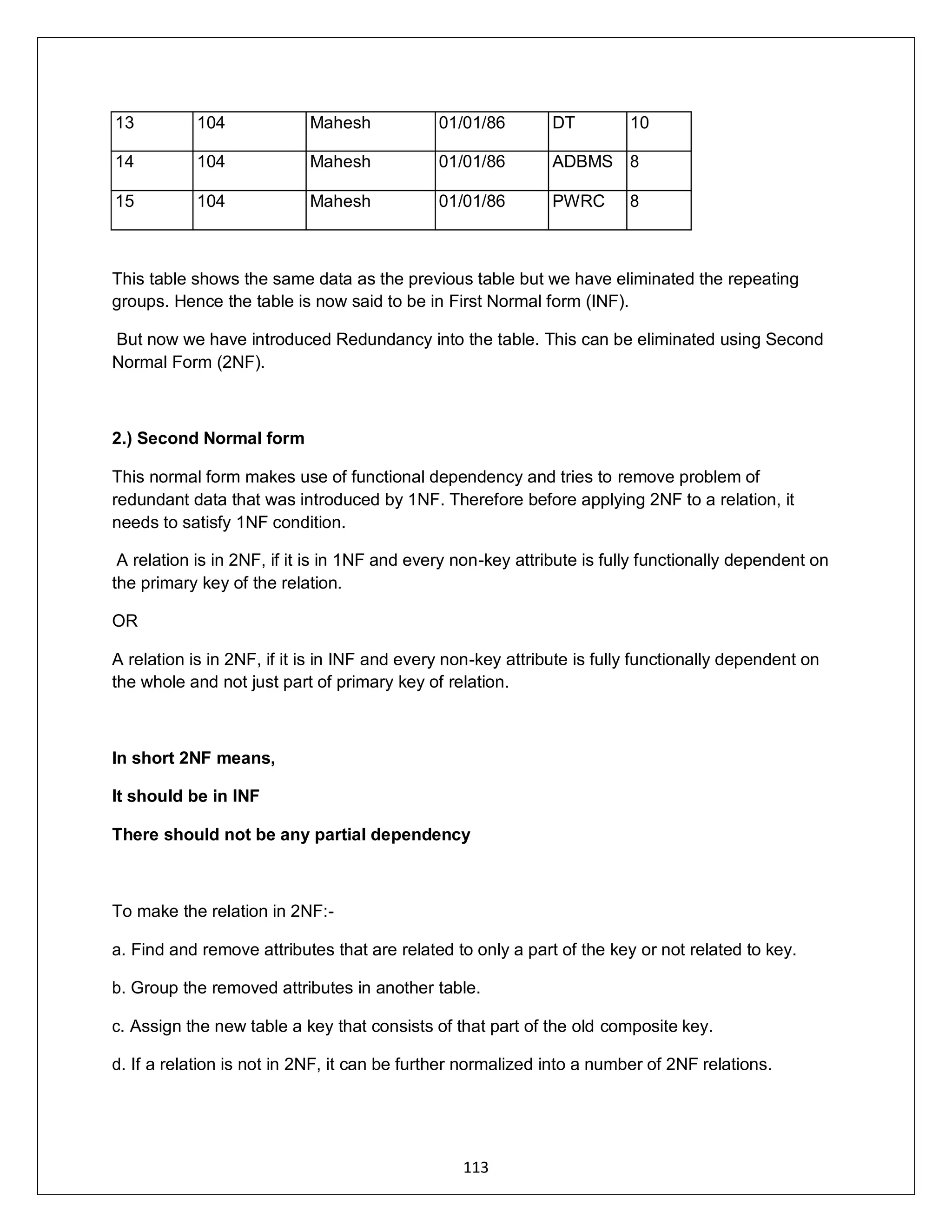
1.) First Normal Form
Simplest form of normalization, simplifies each attribute in relation. This Normal form given by
E.F. Codd (1970) and the later version by C.J. Date (2003)](https://image.slidesharecdn.com/tybsc-csdbms2notes-170810043037/75/Tybsc-cs-dbms2-notes-111-2048.jpg)
![ADDRESS:302 PARANJPE UDYOG BHAVAN,OPP SHIVSAGAR RESTAURANT,THANE [W].PH 8097071144/55
120
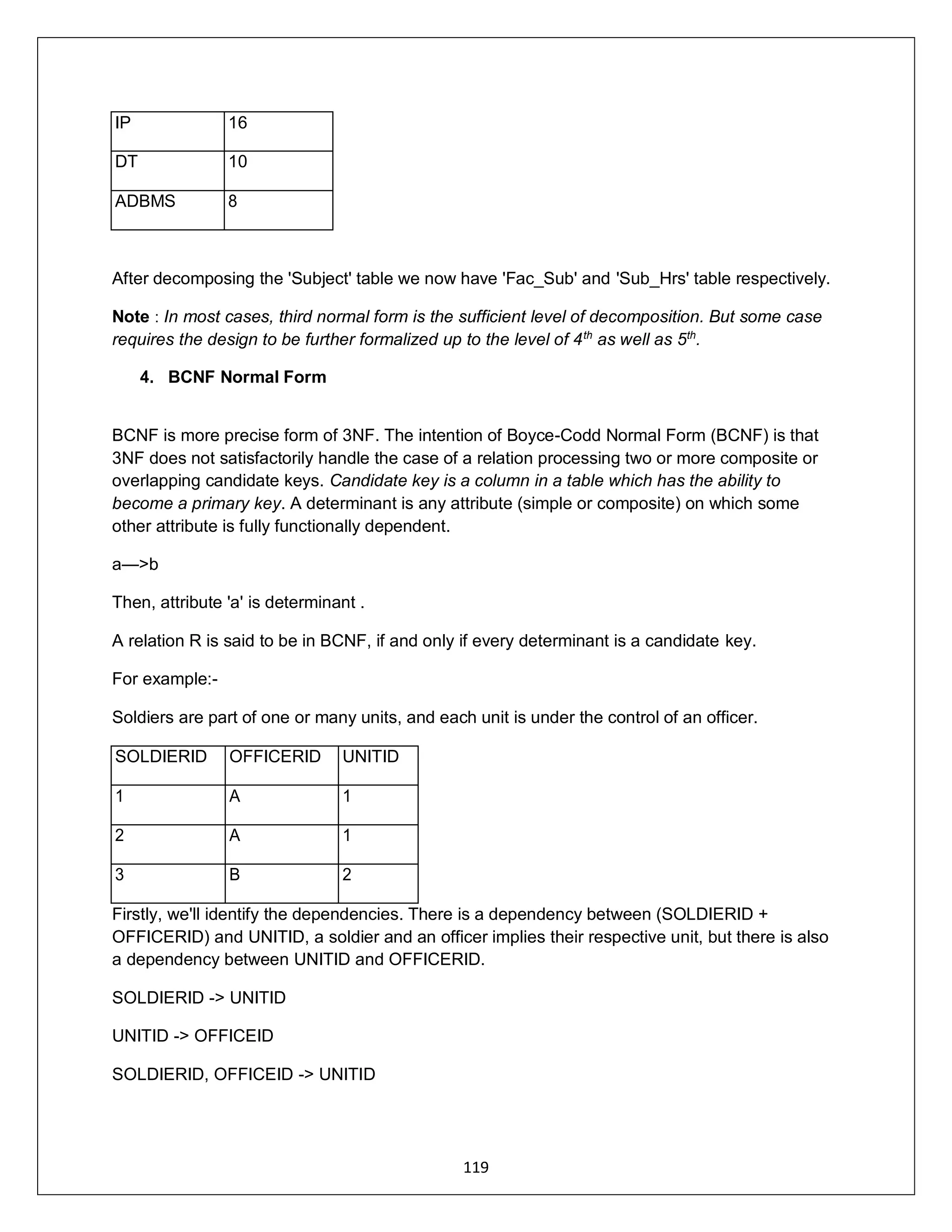
This last dependency however is not partial (dependence on part of a prime attribute), nor
transitive (dependence of a nonprime attribute on another nonprime attribute. What we have is a
table where a determinate in the table is not a candidate key (UNITID). Candidate key are
SOLDERID and OFFICEID.
Thus we can convert the above to BCNF by realizing that a better composite key is one of
SOLDERIERID and UNITID, which creates a dependency between UNITID and OFFICERID,
which is a partial dependency. This is then resolved by dividing the table, the solution being as
follow:
Candidate key (SOLDIERID) and SOLDIERID -> UNITID
Candidate key (UNIT ID) AND UNIT ID -> OFFICEID
UNITID OFFICERID
1 A
1 A
2 B
The above table is now in BCNF.
Q.] Explain Multivalued Dependency and 4th
NF
Multivalued dependency is defined as relationship which accepts the cross product pattern.
Multivalued dependency defined by X —>—> Y is said to hold for a relation
R(X,Y,Z) if for a given set of values of X, there is a set of associated values of attribute Y, and X
values depend only on X values and have no dependence on the set of attributes Z.
SOLDIERID UNITID
1 1
2 1
3 2](https://image.slidesharecdn.com/tybsc-csdbms2notes-170810043037/75/Tybsc-cs-dbms2-notes-121-2048.jpg)
![122
DBP-1 Robert Data Modeling Techniques
DAT-2 Maria Database Advanced
Techniques
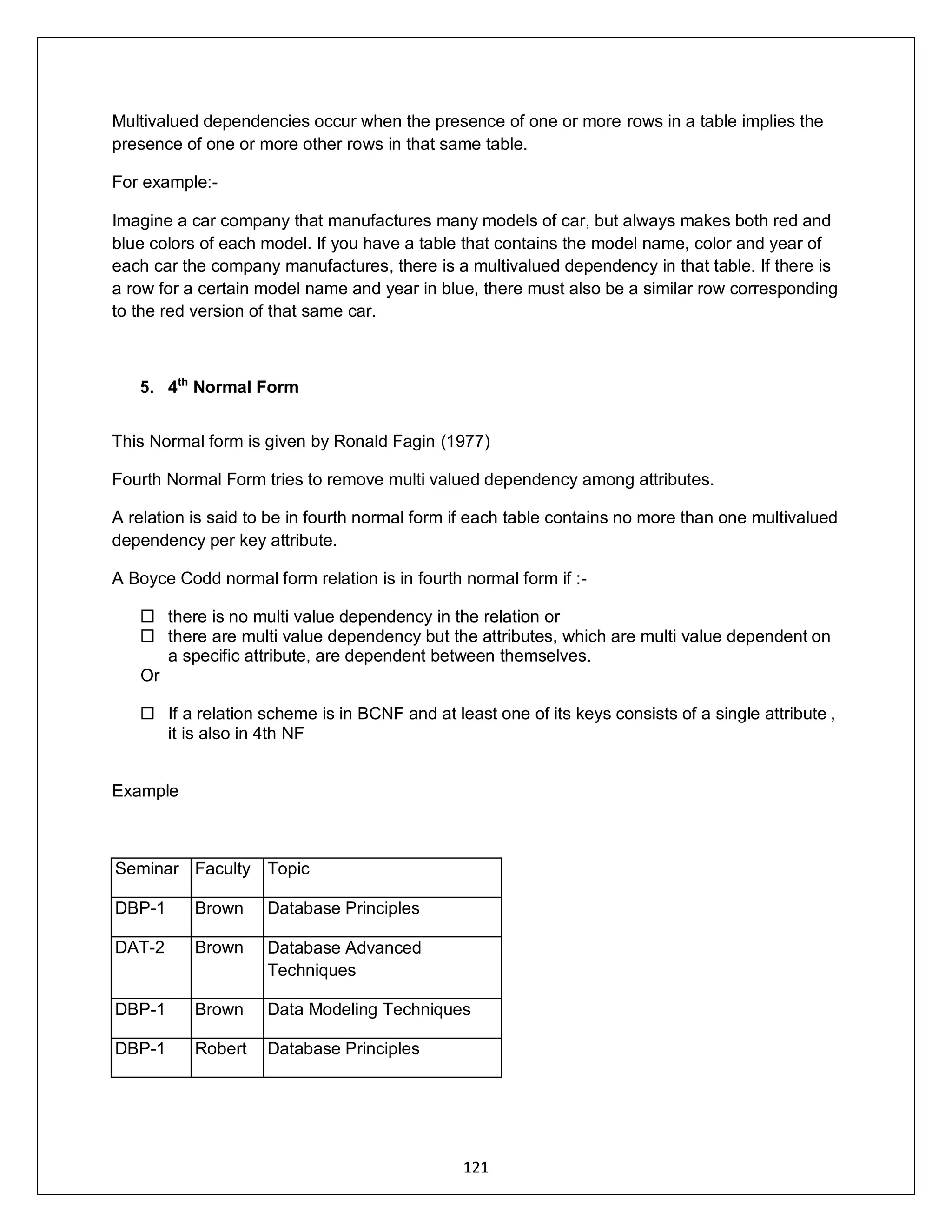
In the above example, same topic is being taught in a seminar by more than 1 faculty and each
Faculty takes up different topics in the same seminar. Hence, Topic names are being repeated
several times. This is an example of multivalued dependency.
To eliminate multivalued dependency, split the table such that there is no multivalued
dependency.
Seminar Topic
DBP-1 Database Principles
DAT-2 Database Advanced Techniques
DBP-1 Data Modeling Techniques
Seminar Faculty
DBP-1 Brown
DAT-2 Brown
DBP-1 Robert
DAT-2 Maria
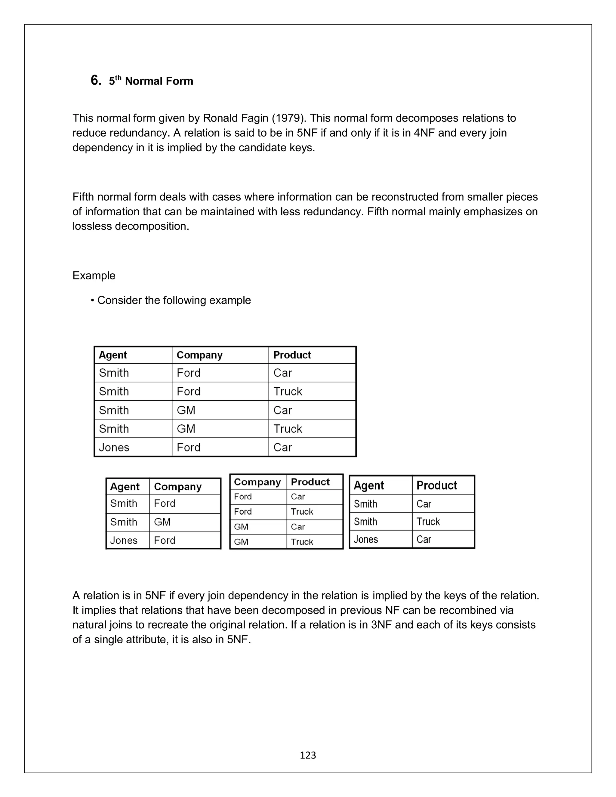
Q.] Explain Join dependency and 5th
NF
A table T is subject to a join dependency if T can always be recreated by joining multiple
tables each having a subset of the attributes of T. If one of the tables in the join has all the
attributes of the table T, the join dependency is called trivial.
The join dependency plays an important role in the 5NF normalization, also known as project-
join normal form](https://image.slidesharecdn.com/tybsc-csdbms2notes-170810043037/75/Tybsc-cs-dbms2-notes-123-2048.jpg)


![ But in the meantime, another transaction might have requested and received a conflicting
lock!
To prevent this, the entire sequence of actions in a lock request call (checking to see if the
request can be granted, updating the lock table, etc.) must be implemented as an atomic
operation.
LOCK Conversions
The DBMS maintains a transaction table, which contains (among other things) a list of the
locks currently held by a transaction.
This list can be checked before requesting a lock, to ensure that the same transaction does
not request the same lock twice.
However, a transaction may need to acquire an exclusive lock on an object for which it
already holds a shared lock. Such a lock upgrade request is handled specially by granting
the write lock immediately if no other transaction holds a shared lock on the object and
inserting the request at the front of the queue otherwise.
The rationale for favoring the transaction thus is that it already holds a shared lock on the
object and queuing it behind another transaction that wants an exclusive lock on the same
object causes both transactions to wait for each other and therefore be blockedforever.
Lock upgrades leads to a deadlocks caused by conflicting upgrade requests.
For example, , if two transactions that hold a shared lock on an object both request an
upgrade to an exclusive lock, this leads to a deadlock because first transaction is waiting for
second to release its lock and other transaction is waiting for first transaction to release its
lock.]
A better approach is to avoid the need for lock upgrades altogether by obtaining exclusive
locks initially and downgrading to a shared lock once it is clear that this issufficient.
For example of an SQL update statement, rows in a table are locked in exclusive mode first.
If a row does not satisfy the condition for being updated, the lock on the row is downgraded
to a shared lock.
The downgrade approach reduces concurrency by obtaining white lock some cases where
they are not require.
On the whole require, however, it improve through put by reducing dead locks.
This approach is therefore widely used current commercial system.
Concurrency can be increase by introducing new kind of lock, called and update lock that is
compatible with shared lock but not other update and exclusive lock.
By setting and update lock initially, rather than exclusive lock, we prevent conflict with read
operation.
Once we are sure we need not update object, we can downgrade to the shared lock.
If we need to update the object, we must first upgrade to an exclusive lock. This upgrade
does not lead to a deadlock because no other transaction can have an upgrade or exclusive
on the object.
Additional Issues: Lock Upgrades, Convoys, Latches
We have concentrated thus far on how the DBMS schedules transactions, based on their
requests for locks. This interleaving interacts with the operating system's scheduling of
processes access to the CPU and can lead to a situation called a convoy, where most of the
CPU cycles are spent on process switching. The problem is that a transaction T holding a](https://crownmelresort.com/image.slidesharecdn.com/tybsc-csdbms2notes-170810043037/75/Tybsc-cs-dbms2-notes-21-2048.jpg)


![ORDER / NOORDER]
Note: - Sequence is always given a name so that it can be referenced later when required.
Keywords And Parameters
INCREMENT BY: Specifies the interval between sequence numbers. It can be any positive or
negative value but not zero. If this clause is omitted, the default value is 1.
MINVALUE: Specifies the sequence minimum value.
NOMINVALUE: Specifies a minimum value of 1 for an ascending sequence and -(10)^26 for a
descending sequence.
MAXVALUE: Specifics the maximum value that a sequence can generate.
NOMAXVALUE: Specifies a maximum of 10^27 for an ascending sequence or -1 for a descending
sequence. This is the default clause.
START WITH: Specifies the first sequence number to be generated. The default for an ascending
sequence is the sequence minimum value (1) and for a descending sequence, it is the maximum
value (-1).
CYCLE: Specifies that the sequence continues to generate repeat values after reaching either its
maximum value.
NOCYCLE: Specifies that a sequence cannot generate more values alter reaching the maximum
value.
CACHE: Specifies how many values of a sequence Oracle pre-allocates and keeps in memory for
faster access. The minimum value for this parameter is two.
NOCACHE: Specifies that values of a sequence are not pre-allocated.
Note: - If the CACHE / NOCACHE clause is omitted ORACLE caches 20 sequence numbers by default.
ORDER: This guarantees that sequence numbers are generated in the order of request. This is only
necessary if using Parallel Server in Parallel mode option. In exclusive mode option, a sequence
always generates numbers in order.
NOORDER: This does not guarantee sequence numbers are generated in order of request. This is
only necessary if you are using Parallel Server in Parallel mode option. If the ORDER/NOORDER
clause is omitted, a sequence takes the NOORDER clause by default.
Note
The ORDER, NOORDER Clause has no significance, if Oracle is configured with Single Server option.](https://crownmelresort.com/image.slidesharecdn.com/tybsc-csdbms2notes-170810043037/75/Tybsc-cs-dbms2-notes-40-2048.jpg)

![ADDR2 VarChar2 50
CITY VarChar2 25
STATE VarChar2 25
PINCODE VarChar2 6
INSERT INTO ADDR_DTLS (ADDR_NO, CODE_NO, ADDR_TYPE, ADDR1, ADDR2, CITY, STATE,
PINCODE) VALUES(ADDR SEQ.NextVal, ‘B5’, ‘B’, ‘Vertex Plaza, Shop 4,’, ‘Western Express Highway,
Dahisar (East),’, ‘Mumbai’, ‘Maharashtra’, ‘400078’);
To reference the current value of a sequence:
SELECT < SequenceNnme >. CurrVal FROM DUAL;
Altering a Sequence
A sequence once created can be altered.
This is achieved by using the ALTER SEQUENCE statement.
Syntax:
ALTER SEQUENCE <SequenceName>
[INCREMENT BY <IntegerValue> MAXVALUE <IntegerValue> / NOMAXVALUE
MINVALUE <IntegerValue> / NOMINVALUE CYCLE / NOCYCLE
CACHE < IntegerVnlue >/ NOCACHE ORDER / NOORDER]
Note
The START value of the sequence cannot be altered.
Example 23:
Change the Cache value of the sequence ADDR_SEQ to 30 and interval between two
numbers as 2.
ALTER SEQUENCE ADDR_SEQ INCREMENT BY 2 CACHE 30;
Dropping A Sequence
The DROP SEQUENCE command is used to remove the sequence from the database.
Syntax:
DROP SEQUENCE < SequenceName > ;](https://crownmelresort.com/image.slidesharecdn.com/tybsc-csdbms2notes-170810043037/75/Tybsc-cs-dbms2-notes-42-2048.jpg)


![ The call to the Oracle engine needs to be made only once to execute number ofstatements.
Oracle engine is called only once for each block, the speed of SQL statement execution is
vastly enhanced, when compared to the Oracle engine being called once for each SQL
statement.
Fundamentals of PL/SQL
The Character Set
Uppercase alphabets(A-Z)
Lowercase alphabets (a-z)
Numerals (0-9)
Symbols
( ) + - * / < > = ! ; : . ‘ @ % , “ # $ ^ & _ { } ? [ ]
Compound symbols used in PL/SQL block are
<> != -= ^= <= >= : = ** || << >>
Literals
Literal is a numeric value or a character string used to represent itself.
Numeric Literal
These can be either integer or floats. If a floats being represented, then the integer part
must be separated from float part by a period.
Example
25, 6.34, -5, 25e-03, .1
Logical (Boolean) Literal
These are predetermined constants. The values that can be assigned to this type are:
TRUE, FALSE, NULL
String Literal
These are represented by one or more legal characters and must be enclosed within
single quotes. The single quote character can be represented, by writing it twice in a
string literal.
Example](https://crownmelresort.com/image.slidesharecdn.com/tybsc-csdbms2notes-170810043037/75/Tybsc-cs-dbms2-notes-46-2048.jpg)
![ ‘Hello world’
‘Don’t go without saving your work’
Character Literal
These are string literals consisting of single characters.
Example
‘*’
‘A’
PL/SQL Datatypes
Predefined Datatypes
Number Types
Character Types
National Character Types
Boolean Types
LOB Types
Date and Interval Types
Number Types
Number types let you store numeric data (integers, real numbers, and floating-point
numbers)
BINARY_INTEGER
We use the BINARY_INTEGER datatype to store signed integers.
BINARY_INTEGER values require less storage than NUMBER values.
BINARY_INTEGER Subtypes
NATURAL - Restrict an integer variable to non-negative or positive values
NATURALN - Prevent the assigning of nulls to an integer variable.
POSITIVE - Restrict an integer variable to non-negative or positive values
POSITIVEN - Prevent the assigning of nulls to an integer variable.
SIGNTYPE - Lets you restrict an integer variable to the values -1, 0, and 1.
NUMBER
We use the NUMBER datatype to store fixed-point or floating-point numbers.
We can specify precision, which is the total number of digits, and scale, which isthe
number of digits to the right of the decimal point. The syntax follows:
NUMBER[(precision,scale)]
To declare fixed-point numbers, for which you must specify scale, use the following
form:
NUMBER(precision,scale)
NUMBER Subtypes
DEC
DECIMAL
NUMERIC
INTEGER
INT](https://crownmelresort.com/image.slidesharecdn.com/tybsc-csdbms2notes-170810043037/75/Tybsc-cs-dbms2-notes-47-2048.jpg)
![ SMALLINT
DOUBLE PRECISION
FLOAT
REAL
Use the subtypes DEC, DECIMAL, and NUMERIC to declare fixed-point numbers with a
maximum precision of 38 decimal digits.
Use the subtypes DOUBLE PRECISION and FLOAT to declare floating-point numbers with a
maximum precision of 126 binary digits, which is roughly equivalent to 38 decimal
digits.
REAL to declare floating-point numbers with a maximum precision of 63 binary digits,
this is roughly equivalent to 18 decimal digits.
Use the subtypes INTEGER, INT, and SMALLINT to declare integers with a maximum
precision of 38 decimal digits.
PLS_INTEGER
You use the PLS_INTEGER datatype to store signed integers
PLS_INTEGER values require less storage than NUMBER values. Also,PLS_INTEGER
operations use machine arithmetic, so they are faster than NUMBER and
BINARY_INTEGER operations.
Character Types
Character types let you store alphanumeric data, represent words and text, and manipulate
character strings.
CHAR
We use the CHAR datatype to store fixed-length character data. How the datais
represented internally depends on the database character set.
Maximum size up to 32767 bytes.
We can specify the size in terms of bytes or characters, where each character contains
one or more bytes, depending on the character set encoding.
CHAR[(maximum_size [CHAR | BYTE] )]
If you do not specify a maximum size, it defaults to 1.
VARCHAR2
You use the VARCHAR2 datatype to store variable-length character data.
VARCHAR2(maximum_size [CHAR | BYTE])](https://crownmelresort.com/image.slidesharecdn.com/tybsc-csdbms2notes-170810043037/75/Tybsc-cs-dbms2-notes-48-2048.jpg)
![ National Character Types
The widely used one-byte ASCII and EBCDIC character sets are adequate to represent the
Roman alphabet, but some Asian languages, such as Japanese, contain thousands of
characters.
These languages require two or three bytes to represent each character.
NCHAR
You use the NCHAR datatype to store fixed-length (blank-padded if necessary) national
character data
The NCHAR datatype takes an optional parameter that lets you specify a maximumsize
in characters. The syntax follows:
NCHAR[(maximum_size)]
NVARCHAR2
You use the NVARCHAR2 datatype to store variable-length Unicode character data.
The NVARCHAR2 datatype takes a required parameter that specifies a maximum sizein
characters. The syntax follows:
NVARCHAR2(maximum_size)
Boolean Type
BOOLEAN
You use the BOOLEAN datatype to store the logical values TRUE, FALSE, and NULL.
Only logic operations are allowed on BOOLEAN variables.
The BOOLEAN datatype takes no parameters.
LOB Types
The LOB (large object) datatypes BFILE, BLOB, CLOB, and NCLOB let you store blocks of
unstructured data (such as text, graphic images, video clips, and sound waveforms) up to
four gigabytes in size.
PL/SQL operates on LOBs through the locators.
BFILE](https://crownmelresort.com/image.slidesharecdn.com/tybsc-csdbms2notes-170810043037/75/Tybsc-cs-dbms2-notes-49-2048.jpg)

![ INTERVAL YEAR TO MONTH
You use the datatype INTERVAL YEAR TO MONTH to store and manipulate intervals of
years and months.
Example,
INTERVAL YEAR[(precision)] TO MONTH
where precision specifies the number of digits in the years field. You cannot
use a symbolic constant or variable to specify the precision; you must use an integer
literal in the range 0 .. 4. The default is 2.
INTERVAL DAY TO SECOND
You use the datatype INTERVAL DAY TO SECOND to store and manipulate intervals
of days, hours, minutes, and seconds.
The syntax is:
INTERVAL DAY[(leading_precision)] TO
SECOND[(fractional_seconds_precision)]
where leading_precision and fractional_seconds_precision specify the number of digits
in the days field and seconds field, respectively. In both cases, you cannot use a
symbolic constant or variable to specify the precision; you must use an integer
literal in the range 0 .. 9. The defaults are 2 and 6, respectively.
VARIABLES
Variables may be used to store the result of a query or calculations. Variables must be
declared before being used.
Variable Name
A variable name must begin with a character.
Variable length is 30 Characters.
Reserved words can not be used as variable names unless enclosed within the double
quotes.
Variables must be separated from each other by at least one space or by a punctuation
mark.
The case (upper/lower) is insignificant when declaring variable names.
Space can not be used in variable name.
Declaring variables](https://crownmelresort.com/image.slidesharecdn.com/tybsc-csdbms2notes-170810043037/75/Tybsc-cs-dbms2-notes-51-2048.jpg)
![ We can declare a variable of any data type either native to the ORACLE or native to
PL/SQL.
Variables are declared in the DECLARE section of the PL/SQL block.
. Declaration involves the name of the variable followed by its data type followed by
semicolon (;).
To assign a value to the variable the assignment operator (:=) is used.
Syntax:
<Variable name> <type> [ :=<value> ];
Example:
Ename CHAR(10);
Assigning value to a variable
There are two ways to assign a value to a variable.
Using the assignment operator ( := )
Ex: sal := 1000.00;
Total_sal := sal – tax;
Selecting or fetching table data values in to variables.
Ex: SELECT sal INTO pay
FROM Employee WHERE emp_id = ‘E001’;
CONSTANT
A variable can be modified, a constant cannot.
Declaring Constant
Declaring a constant is similar to declaring a variable except that you have toadd
the key word CONSTANT and immediately assign a value toit.
Syntax:
<variable_name> CONSTANT <datatype> := <value>;
Example:
Pi CONSTANT NUMBER(3,2) := 3.14;
USE OF %TYPE
While creating a table user attaches certain attributes like data type and constraints.
These attributes can be passed on to the variables being created in PL/SQL using %TYPE
attribute.
This simplifies the declaration of variables and constants.](https://crownmelresort.com/image.slidesharecdn.com/tybsc-csdbms2notes-170810043037/75/Tybsc-cs-dbms2-notes-52-2048.jpg)


![LIKE OPERATOR
LIKE Operator is a Pattern matching operator.
It is used to compare a character string against a pattern.
Wild card characters:
o Percentage sign (%) - It matches any number of characters in a string.
o Underscore ( _ ) - It matches exactly one character.
Example:
SELECT EName FROM Employee WHERE EName LIKE ‘P%’;
It displays EName field of Employee table where ENames starts with P.
IN OPERATOR
It checks to see if a value lies within a specified list of values.
IN operator returns a BOOLEAN result, either TRUE or FALSE.
Syntax:
The_value [NOT] IN (value1, value2, value3……)
Example:
3 IN (4, 8, 7, 5, 3, 2) Returns TRUE
BETWEEN
It checks to see if a value lies within a specified range of value.
Low_End and Upper_Ends are inclusive.
Syntax:
the_value [NOT] BETWEEN low_end AND high_end.
Example:
5 BETWEEN –5 AND 10. Returns TRUE
IS NULL
It checks to see if a value is NULL.
Syntax:
Example:
the_value IS [NOT] NULL
IF balance IS NULL THEN](https://crownmelresort.com/image.slidesharecdn.com/tybsc-csdbms2notes-170810043037/75/Tybsc-cs-dbms2-notes-55-2048.jpg)


![BEGIN
/* Initialize the radius to 3, since calculations are required for radius 3 to 7 */
radius := 3;
/* Set a loop so that it fires till the radius value reaches 7 */
WHILE RADIUS <= 7
LOOP
/* Area calculation for a circle */
area := pi * power(radius,2);
/* Insert the value for the radius and its corresponding area calculated in the table */
INSERT INTO areas VALUES (radius, area);
END;
/* Increment the value of the variable radius by 1 */
radius := radius + 1;
END LOOP;
FOR LOOP
The FOR LOOP enables you to execute a loop for predetermined number of times.
The variable in the FOR loop need not be declared.
The increament value can not be specified.
The for loop variable is always incremented by 1.
Reverse is an optional keyword. If we specify keyword reverse then variable
considers last value first and then decrement it to get the start value.
The syntax for FOR LOOP is as follows:
FOR var IN [REVERSE] start…end
LOOP
Statements;
END LOOP;](https://crownmelresort.com/image.slidesharecdn.com/tybsc-csdbms2notes-170810043037/75/Tybsc-cs-dbms2-notes-62-2048.jpg)


![END IF;
CASE Expression
A CASE expression selects a result from one or more alternatives, and returnsthe
result.
The CASE expression uses a selector, an expression whose value determineswhich
alternative to return.
A CASE expression has the following form:
CASE selector
WHEN expression1 THEN result1
WHEN expression2 THEN result2
...
WHEN expressionN THEN resultN
[ELSE resultN+1]
END;
The selector is followed by one or more WHEN clauses, which are checked
sequentially.
The value of the selector determines which clause is executed.
The first WHEN clause that matches the value of the selector determines the result
value, and subsequent WHEN clauses are not evaluated.
An example follows:
DECLARE
grade CHAR(1) := 'B';
appraisal VARCHAR2(20);
BEGIN
appraisal :=
CASE grade
WHEN 'A' THEN 'Excellent'
WHEN 'B' THEN 'Very Good'
WHEN 'C' THEN 'Good'
WHEN 'D' THEN 'Fair'
WHEN 'F' THEN 'Poor'
ELSE 'No such grade'
END;
END;
The optional ELSE clause works similarly to the ELSE clause in an IF statement.
If the value of the selector is not one of the choices covered by a WHEN clause, the
ELSE clause is executed.](https://crownmelresort.com/image.slidesharecdn.com/tybsc-csdbms2notes-170810043037/75/Tybsc-cs-dbms2-notes-66-2048.jpg)
![If no ELSE clause is provided and none of the WHEN clauses are matched, the
expression returns NULL.
Searched CASE Expression
PL/SQL also provides a searched CASE expression, which has the form:
CASE
WHEN search_condition1 THEN result1
WHEN search_condition2 THEN result2
...
WHEN search_conditionN THEN resultN
[ELSE resultN+1]
END;
A searched CASE expression has no selector.
Each WHEN clause contains a search condition that yields a Boolean value, which lets
you test different variables or multiple conditions in a single WHEN clause.
An example follows:
DECLARE
grade CHAR(1);
appraisal VARCHAR2(20);
BEGIN
...
appraisal :=
CASE
WHEN grade = 'A' THEN 'Excellent'
WHEN grade = 'B' THEN 'Very Good'
WHEN grade = 'C' THEN 'Good'
WHEN grade = 'D' THEN 'Fair'
WHEN grade = 'F' THEN 'Poor'
ELSE 'No such grade'
END;
...
END;
The search conditions are evaluated sequentially.
The Boolean value of each search condition determines which WHEN clause is
executed.
If a search condition yields TRUE, its WHEN clause is executed.
After any WHEN clause is executed, subsequent search conditions are not evaluated.
If none of the search conditions yields TRUE, the optional ELSE clause is executed.](https://crownmelresort.com/image.slidesharecdn.com/tybsc-csdbms2notes-170810043037/75/Tybsc-cs-dbms2-notes-67-2048.jpg)

![CASE
WHEN search_condition1 THEN sequence_of_statements1;
WHEN search_condition2 THEN sequence_of_statements2;
...
WHEN search_conditionN THEN sequence_of_statementsN;
[ELSE sequence_of_statementsN+1;]
END CASE;
The searched CASE statement has no selector.
Its WHEN clauses contain search conditions that yield a Boolean value,not
expressions that can yield a value of any type.
The search conditions are evaluated sequentially.
The Boolean value of each search condition determines which WHEN clause is
executed.
If a search condition yields TRUE, its WHEN clause is executed. If any WHEN clause
is executed, control passes to the next statement, so subsequent search conditions
are not evaluated.
If none of the search conditions yields TRUE, the ELSE clause is executed. The ELSE
clause is optional. However, if you omit the ELSE clause, PL/SQL adds the following
implicit ELSE clause:
An example follows:
CASE
WHEN grade = 'A' THEN dbms_output.put_line('Excellent');
WHEN grade = 'B' THEN dbms_output.put_line('Very Good');
WHEN grade = 'C' THEN dbms_output.put_line('Good');
WHEN grade = 'D' THEN dbms_output.put_line('Fair');
WHEN grade = 'F' THEN dbms_output.put_line('Poor');
ELSE dbms_output.put_line('No such grade');
END CASE;
Handling Null Values in Comparisons and Conditional Statements
When working with nulls, you can avoid some common mistakes by keeping in mind the following
rules:
Comparisons involving nulls always yield NULL
Applying the logical operator NOT to a null yields NULL
In conditional control statements, if the condition yields NULL, its associated sequence of
statements is not executed
If the expression in a simple CASE statement or CASE expression yields NULL, it cannot be
matched by using WHEN NULL. In this case, you would need to use the searched case syntax
and test WHEN expression IS NULL.](https://crownmelresort.com/image.slidesharecdn.com/tybsc-csdbms2notes-170810043037/75/Tybsc-cs-dbms2-notes-69-2048.jpg)

![ORACLE TRANSACTIONS
PL / SQL TRANSACTIONS
A series of one or more SQL statements that are logically related or a series of operations
performed on Oracle table data is termed as a Transaction.
Oracle treats this logical unit as a single entity.
Oracle treats changes to table data as a two-step process. First, the changes requested are
done.
To make these changes permanent a COMMIT statement has to be given at the SQL
prompt.
A ROLLBACK statement given at the SQL prompt can be used to undo a part of or the entire
transaction.
Specifically, a transaction is a group of events that occur between any of the following
events:
Connecting to Oracle
Disconnecting from Oracle
Committing changes to the database table
Rollback
Closing Transactions
A transaction can be closed by using either a commit or a rollback
statement.
By using these statements. table data can be changed or all the changes made
to the table data undone.
Using COMMIT:
A COMMIT ends the current transaction and makes permanent any changes made
during the transaction.
All transactional locks acquired on tables are released.
Syntax:
COMMIT;
Using ROLLBACK:
A ROLLBACK does exactly the opposite of COMMIT.
It ends the transaction but undoes any changes made during the transaction.
All transactional locks acquired on tables are released.
Syntax:
ROLLBACK [WORK] [TO [SAVEPOINT] <SavePointName>];
where,
WORK Is optional and is provided for ANSI compatibility](https://crownmelresort.com/image.slidesharecdn.com/tybsc-csdbms2notes-170810043037/75/Tybsc-cs-dbms2-notes-71-2048.jpg)


![SELECT … FOR UPDATE with NOWAIT Option
In order to avoid unnecessary waiting time, a NOWAIT option can be used to inform the Oracle
engine to terminate the SQL statement if the record has already been locked. If this happens the
Oracle engine terminates the running DML and comes up with a message indicating that the
resource is busy.
If Client B fires the following select statement now with a NOWAIT clause:
Client B> SELECT * FROM ACCT_MSTR WHERE ACCT_NO ='SB9' FOR UPDATE NOWAIT;
Output:
Since Client A has already locked the record SB9 when Client B tries to acquire a shared
lock on the same record the Oracle Engine displays the following message:
SQL> 00054: resource busy and acquire with nowait specified.
The SELECT ... FOR UPDATE cannot be used with the following:
Distinct and the Group by clause
Set operators and Group functions
Using Lock Table Statement
To manually override Oracle's default locking strategy by creating a data lock in a specific
mode.
Syntax:
LOCK TABLE <TabIeName> [, <TabIeName>] ...
IN {ROW SHARE|ROW EXCLUSIVEISHARE UPDATE|
SHAREISHARE ROW EXCLUSIVE I EXCLUSIVE }
[NOWAIT]
where,
TableName Indicates the name of table(s), view(s) to be locked. In
case of views, the lock is placed on underlying tables.
IN Decides what other locks on the same resource can
exist simultaneously. For example, if there is an
exclusive lock on the table no user can update rows in
the table. It can have any of the following values:
Exclusive: They allow query on the locked resource but prohibit](https://crownmelresort.com/image.slidesharecdn.com/tybsc-csdbms2notes-170810043037/75/Tybsc-cs-dbms2-notes-79-2048.jpg)


![| record_type_name
| ref_cursor_type_name
}];
ref_cursor_variable_declaration ::=
cursor_variable_name type_name;
Keyword and Parameter Description
cursor_name
o An explicit cursor previously declared within the current scope.
cursor_variable_name
o A PL/SQL cursor variable previously declared within the current scope.
db_table_name
o A database table or view, which must be accessible when the declaration is
elaborated.
record_name
o A user-defined record previously declared within the current scope.
record_type_name
o A user-defined record type that was defined using the datatype specifier RECORD.
REF CURSOR
o Cursor variables all have the datatype REF CURSOR.
RETURN
o Specifies the datatype of a cursor variable return value. You can use the %ROWTYPE
attribute in the RETURN clause to provide a record type that represents a row in a
database table, or a row from a cursor or strongly typed cursor variable. You can use
the %TYPE attribute to provide the datatype of a previously declared record.
Types of Cursor Variables
REF CURSOR types can be strong (with a return type) or weak (with no return type).
Strong REF CURSOR types are less error prone because the PL/SQL compiler lets you
associate a strongly typed cursor variable only with queries that return the right set of
columns.
Weak REF CURSOR types are more flexible because the compiler lets you associate a weakly
typed cursor variable with any query.
Because there is no type checking with a weak REF CURSOR, all such types are
interchangeable. Instead of creating a new type, you can use the predefinedtype
SYS_REFCURSOR.
The following procedure opens the cursor variable generic_cv for the chosen query:
PROCEDURE open_cv (generic_cv IN OUT GenericCurTyp,choice NUMBER) IS
BEGIN](https://crownmelresort.com/image.slidesharecdn.com/tybsc-csdbms2notes-170810043037/75/Tybsc-cs-dbms2-notes-94-2048.jpg)


![The process of decomposition of a relation R into a set of relations R1, R2....Rn is based on
identifying attributes and using that as a basis of decomposition.
R=R1 U R2 U………Rn.
This is a process of dividing one table into multiple tables using projection operator.
We may decompose tables into vertical segments. Vertical fragmentation is done with help of
projection operator. By taking projection of original table we can create multiple vertically
fragmented tables.
Original table
Decomposition
Q.] Explain decomposition?
If a relation is not in the normal form and we wish the relation to be normalized so that some of
the anomalies (like insert, update or delete anomalies) can be eliminated, it is necessary to
decompose the relation in two or more relations.
Eno Ename Class
1 Mahesh BE
2 Yogesh SE
3 Amit TE
Vertically Decomposed
Tables
Eno Ename
1 Mahesh
2 Yogesh
3 Amit
Eno Class
1 BE
2 SE
3 TE](https://crownmelresort.com/image.slidesharecdn.com/tybsc-csdbms2notes-170810043037/75/Tybsc-cs-dbms2-notes-100-2048.jpg)
![Q.] Explain the desirable Properties of decomposition:
The main properties of decomposition are as listed below,
a. Lossless-join decomposition
b. Dependency preservation
c. Lack of redundancy (Repetition of information)
1) Lossless join decomposition
It is clear that decomposition must be lossless so that we do not lose any information from the
relation that is decomposed. Lossless join decomposition ensures that we can never get the
situation where false tuple are generated in relation. For every value on the join attributes there
should be a unique tuple in one of the relations. For following table to become lossless we need
to go for following steps.
Deptjd Dname Stud_Id Sname Location
10 Development 1 Sushant Mahim
20 Teaching 2 Snehal Vashi
30 HR 3 Pratiksha Warli
20 Admin 4 Supraja Dadar
a.Let R1 and R2 form decomposition of relation R.
b.Decompose the relation schema Department-Student into
Department-schema = (Dept_Id, Dname)
Student-schema = (Stud_id, Sname, Location)
c. The attributes in common must be a key for one of the relation for decomposition to be
lossless. R1 ∩ R2 ≠ Φ. There must not be null.](https://crownmelresort.com/image.slidesharecdn.com/tybsc-csdbms2notes-170810043037/75/Tybsc-cs-dbms2-notes-101-2048.jpg)

![3) Lack of Redundancy ( Repetition of information)
Decomposition that we have done should not suffer from any repetition of information problem.
For eg: STUDENT and SECTION data are separated into distinct relations. Thus we do not
have to repeat STUDENT data for each SECTION.
If a single SECTION is made into several STUDENTS, we do not have to repeat the SECTION
data for each STUDENT.
IT is desirable not to have any redundancy in database. This property may be achieved by
normalization process.
Q.] What is a Lossy- join decomposition?
We decomposed a relation intuitively but, still we need a better basis for deciding
decompositions since intuition may not always be correct. A careless decomposition may lead
to problems like loss of information.
Department-Student Schema = (Dept_Id, Dname, Stud_Id, Sname, Location)
Deptjd Dname Stud_Id Sname Location
10 Development 1 Sushant Mahim
20 Teaching 2 Snehal Vashi
30 HR 3 Pratiksha Warli
20 Admin 4 Supraja Dadar
Suppose we decompose the above relation into two relations Department and Student as
follows :](https://crownmelresort.com/image.slidesharecdn.com/tybsc-csdbms2notes-170810043037/75/Tybsc-cs-dbms2-notes-103-2048.jpg)
![Schema 2: Student Schema contains (Stud_Id, Sname, Location)
All the information that was in the relation 'Department' appears to be still available in
'Department-Student' schema but this is not so. Suppose, we would need to join 'Department'
and 'Student' table this join becomes lossy join decomposition.
As R, n R2 = O
So, there is no column common between them, therefore joining not possible. A lossless
decomposition is that which guarantees that the join will result in exactly the same relation as
was decomposed
.
Q.] Explain Functional Dependency:
Schema 1: Department Schema containing (Deptjd, Dname)
Deptjd Dname
10 Development
20 Teaching
30 HR
Studjd Sname Location
1 Sushant Mahim
2 Snehal Vashi
3 Pratiksha Warli
4 Supraja Dadar
The concept of functional dependency is given by E. F. Codd which is also called as
normalization process. This concept is used to define various normal forms.](https://crownmelresort.com/image.slidesharecdn.com/tybsc-csdbms2notes-170810043037/75/Tybsc-cs-dbms2-notes-104-2048.jpg)
![Functional dependency is a type of constraints exists between multiple attributes of a relation.
Functional Dependency (FD) determines the set of values or the attribute based on another
attribute
It is denoted by (—>)
This form can be written as Y is functionally dependent on X or X determines Y.
E code —> E Name
We can say column X is functionally dependent on other column Y. If data value in column X
change when data value in another column Y is modified.
an FD X Y essentially says that if two tuples agree on the values in attributes X, they must
also agree on the values in attributes Y.
Functional Dependency provides a formal mechanism to express constraints between various
attributes of a relation.
For Eg, let us say in below table if the name of employee is changed its ID also need to be
changed so, we can say NAME column is dependent on employee ID column, i.e. For different
name of employee different ID is given.
Employee Table
ID Name
• a • •
MahOOl Mahesh ....
Q.] Explain the Types of Functional Dependencies
1. Full Functional Dependency:
A Functional Dependency A —> B is a full functional dependency if removal of any attributes
from A means that the dependency does not hold any more.
Example](https://crownmelresort.com/image.slidesharecdn.com/tybsc-csdbms2notes-170810043037/75/Tybsc-cs-dbms2-notes-105-2048.jpg)
![{Emp_no, Project_no} -> HOURS i.e. Emp_no —> Hours and Project_no —> Hours
In the above example, Hours is fully functionally dependent on both Emp_no and Project_no.
The number of hours spent on the project by a particular employee cannot be determined with
the project number (Project_no) alone. It needs the employee number (Emp_no) as well.
2. Partial Functional Dependency:
A partial dependency means that a non key column is depend on some columns in composite
primary key of a table. An FD A —> B is a partial dependency if there is some attribute X € A (X
subset of A), that can be removed from A and the dependency will still hold.
Example
{Emp_no, Project_no} —> Ename that is, Emp_no —> Ename
In the above example, Ename is partially dependent on {Emp_no, Project_no} since employee
name (ename) can be determined using the employee id (Emp_no) alone even if project_no is
removed from the relation.
Note: For a table to be in 2nd Normal form there should be no partial dependencies.
Q.] Explain Transitive Dependency
This concept is used when there is redundancy in database. If changing any non key column
(column other then key column) causes change in other non key column in such situations you
may have transitive dependency.
When one non key attribute is functionally dependent on another non key attribute then such a
dependency is called as transitive dependency.
Non Key Attribute —» Non Key Attribute
An FD X —>Y in a relation R is a transitive dependency, if there is a set of attributes Z that is
not a subset of any key of R, and both X —» Z and Z —> Y holds true.
For eg:
EMP_DEPT {Eno, Ename, Dnumber, DeptMgrNo}
Eno —> DeptmgrNo is transitive](https://crownmelresort.com/image.slidesharecdn.com/tybsc-csdbms2notes-170810043037/75/Tybsc-cs-dbms2-notes-106-2048.jpg)
![Dependency of DeptMgrNo on key attribute Eno is transitive as DeptMgrNo depends on
Dnumber and DNumber itself is dependent on Eno.
Eno —> Dnumber and Dnumber —> DMgrNo
Q.] Armstrong's Axioms - Closures of Functional Dependency
Given that A, B and C are sets of attributes in a relation R; one can derive several properties of
functional dependencies.
Axioms are nothing but rules of inference which provides a simple technique for reasoning
about functional dependencies.
1) Primary Rules
a. Subset Property (Axiom of Reflexivity)
If Y is a subset of X, then X —» Y
b. Augmentation (Axiom of Augmentation)
If X —> Y, then XZ -> YZ
c. Transitivity (Axiom of Transitivity)
If X -> Y and Y -> Z, then X -> Z
2) Secondary Rules (Based on above rules)
a. Union: If X -» Y and X -> Z, then X -> YZ
b. Decomposition: If X —> YZ and X -> Y, then X -> Z
c. Pseudo Transitivity: If X —> Y and YZ -> W, then XZ -> W
Example : Consider relation R = (A,B,C,D,E,F) having set of FD's
A -> B A-> C](https://crownmelresort.com/image.slidesharecdn.com/tybsc-csdbms2notes-170810043037/75/Tybsc-cs-dbms2-notes-107-2048.jpg)

![AC->F
Therefore, AC->DF
Normalization
Normalization is a step by step decomposition of complex records into simple records.
Normalization results in tables that satisfy some constraints and are represented in a simple
manner. This process is also called as canonical synthesis. This is a relational database
design process to avoid data redundancy by applying some constraints on data to avoid various
data anomalies.
For E.g. If same information is repeated in multiple tables of database then there are chances
that these tables will not be consistent in case of data updation, insertion or deletion. This
instance may lead to problems of data integrity. A normalized table is less vulnerable to such
data anomalies.
Normalization is a process of designing a consistent database by minimizing redundancy
and ensuring data integrity through decomposition which is lossless.
Q.] Goals/ Importance of Database Normalization
1. Ensures Data Integrity
Data integrity ensures the correctness of data stored within the database. It is achieved by
imposing integrity constraints. An integrity constraint is a rule, which restricts values present in
the database.
There are three integrity constraints:
(i) Entity constraints: The entity integrity rule states that the value of the primary key can never
be a null value. Because a primary key is used to identify a unique row in a relational table, its
value must always be specified and should never be unknown.The integrity rule requires that
insert, update and delete operations maintain the uniqueness and existence of all primarykeys.](https://crownmelresort.com/image.slidesharecdn.com/tybsc-csdbms2notes-170810043037/75/Tybsc-cs-dbms2-notes-109-2048.jpg)
![(ii) Domain Constraints: Only permissible values of an attribute are allowed in a relation.
(iii) Referential Integrity constraints: The referential integrity rule states that if a relational
table has a foreign key, then every value of the foreign key must either be null or match the
values in the relational table (referenced table) in which that foreign key is a primary key.
2.) Prevents Redundancy in data: A non-normalized database is vulnerable to data
anomalies, if it stores data redundantly. If data is stored in two locations, but the data is updated
in only one of the locations, then that data becomes inconsistent. A normalized database stores
non-primary key data in only one location.
3.) To avoid Data Anomaly: A non-normalized table can suffer from logical inconsistencies of
various types, and from data anomalies. A Relational database table should be designed in
such a way that it will avoid all data anomalies.
Q.] Which are the different anomalies related to normalization:-
1) Update anomaly: Same information can be present in multiple records of various relations;
updates to only one table may result in logical inconsistencies.
Example each record in an "Emp_Salary" table might contain an Emp_ID, Ename, Address,
Salary. Thus a change of address for a particular Employee will potentially need to be applied to
multiple tables such as Employee table. If all the records are not updated then some tables may
leave in an inconsistent state.
2) An insertion anomaly: There is a possibility in which certain facts cannot be recorded at all
or they are not yet recorded.
Example
Consider a table, Faculty (Faculty_ID, FName, Subject_Code, Subject, Class). We can add the
details of any faculty member who teaches for a certain subject in a certain class, but we cannot
record the details of a new faculty member who has not yet been assigned to teach any subject
or class. So, subject and class column may be empty initially. If data deleted from one table all
relevant data must also be deleted or redundant.](https://crownmelresort.com/image.slidesharecdn.com/tybsc-csdbms2notes-170810043037/75/Tybsc-cs-dbms2-notes-110-2048.jpg)
![110
3) Deletion Anomaly: If data deleted from one table all relevant data in another related tables
must also be deleted otherwise it will create redundancy problem. Deletion of some data from a
relation necessitates the deletion of some unrelated data also called as deletion anomaly.
Example
In the previous example, the table suffers from this type of anomaly. If a faculty member
temporarily ceases to be assigned a subject, we must delete the entire record on which that
faculty member appears.
Normal Forms
Forms are designed to logically address potential problems such as inconsistencies and
redundancy in information stored in the database. A database is said to be in one of the Normal
Forms, if it satisfies the rules required by that form as well as the previous form; it also will not
suffer from any of the problems addressed by the form.
Q.] State and explain Types of Normal Forms
a. First normal form (INF)
b. Second normal form (2NF)
c. Third normal form (3NF)
d. Boyce-Codd normal form (BCNF)
e. Fourth normal form (4NF)
f. Fifth Normal Form (5NF)
1.) First Normal Form
Simplest form of normalization, simplifies each attribute in relation. This Normal form given by
E.F. Codd (1970) and the later version by C.J. Date (2003)](https://crownmelresort.com/image.slidesharecdn.com/tybsc-csdbms2notes-170810043037/75/Tybsc-cs-dbms2-notes-111-2048.jpg)


![ADDRESS:302 PARANJPE UDYOG BHAVAN,OPP SHIVSAGAR RESTAURANT,THANE [W].PH 8097071144/55
120
This last dependency however is not partial (dependence on part of a prime attribute), nor
transitive (dependence of a nonprime attribute on another nonprime attribute. What we have is a
table where a determinate in the table is not a candidate key (UNITID). Candidate key are
SOLDERID and OFFICEID.
Thus we can convert the above to BCNF by realizing that a better composite key is one of
SOLDERIERID and UNITID, which creates a dependency between UNITID and OFFICERID,
which is a partial dependency. This is then resolved by dividing the table, the solution being as
follow:
Candidate key (SOLDIERID) and SOLDIERID -> UNITID
Candidate key (UNIT ID) AND UNIT ID -> OFFICEID
UNITID OFFICERID
1 A
1 A
2 B
The above table is now in BCNF.
Q.] Explain Multivalued Dependency and 4th
NF
Multivalued dependency is defined as relationship which accepts the cross product pattern.
Multivalued dependency defined by X —>—> Y is said to hold for a relation
R(X,Y,Z) if for a given set of values of X, there is a set of associated values of attribute Y, and X
values depend only on X values and have no dependence on the set of attributes Z.
SOLDIERID UNITID
1 1
2 1
3 2](https://crownmelresort.com/image.slidesharecdn.com/tybsc-csdbms2notes-170810043037/75/Tybsc-cs-dbms2-notes-121-2048.jpg)

![122
DBP-1 Robert Data Modeling Techniques
DAT-2 Maria Database Advanced
Techniques
In the above example, same topic is being taught in a seminar by more than 1 faculty and each
Faculty takes up different topics in the same seminar. Hence, Topic names are being repeated
several times. This is an example of multivalued dependency.
To eliminate multivalued dependency, split the table such that there is no multivalued
dependency.
Seminar Topic
DBP-1 Database Principles
DAT-2 Database Advanced Techniques
DBP-1 Data Modeling Techniques
Seminar Faculty
DBP-1 Brown
DAT-2 Brown
DBP-1 Robert
DAT-2 Maria
Q.] Explain Join dependency and 5th
NF
A table T is subject to a join dependency if T can always be recreated by joining multiple
tables each having a subset of the attributes of T. If one of the tables in the join has all the
attributes of the table T, the join dependency is called trivial.
The join dependency plays an important role in the 5NF normalization, also known as project-
join normal form](https://crownmelresort.com/image.slidesharecdn.com/tybsc-csdbms2notes-170810043037/75/Tybsc-cs-dbms2-notes-123-2048.jpg)


The document discusses transactions in database management systems and the ACID properties that transactions must satisfy. It describes the four ACID properties - atomicity, consistency, isolation, and durability. Atomicity ensures that transactions are treated as an atomic unit and either fully occur or not at all. Consistency requires that transactions alone preserve the consistency of the database. Isolation ensures that concurrently executing transactions are isolated from each other. Durability means the effects of committed transactions persist even if the system crashes. The document also discusses transaction schedules, concurrency control, and anomalies that can occur with concurrent transaction execution.