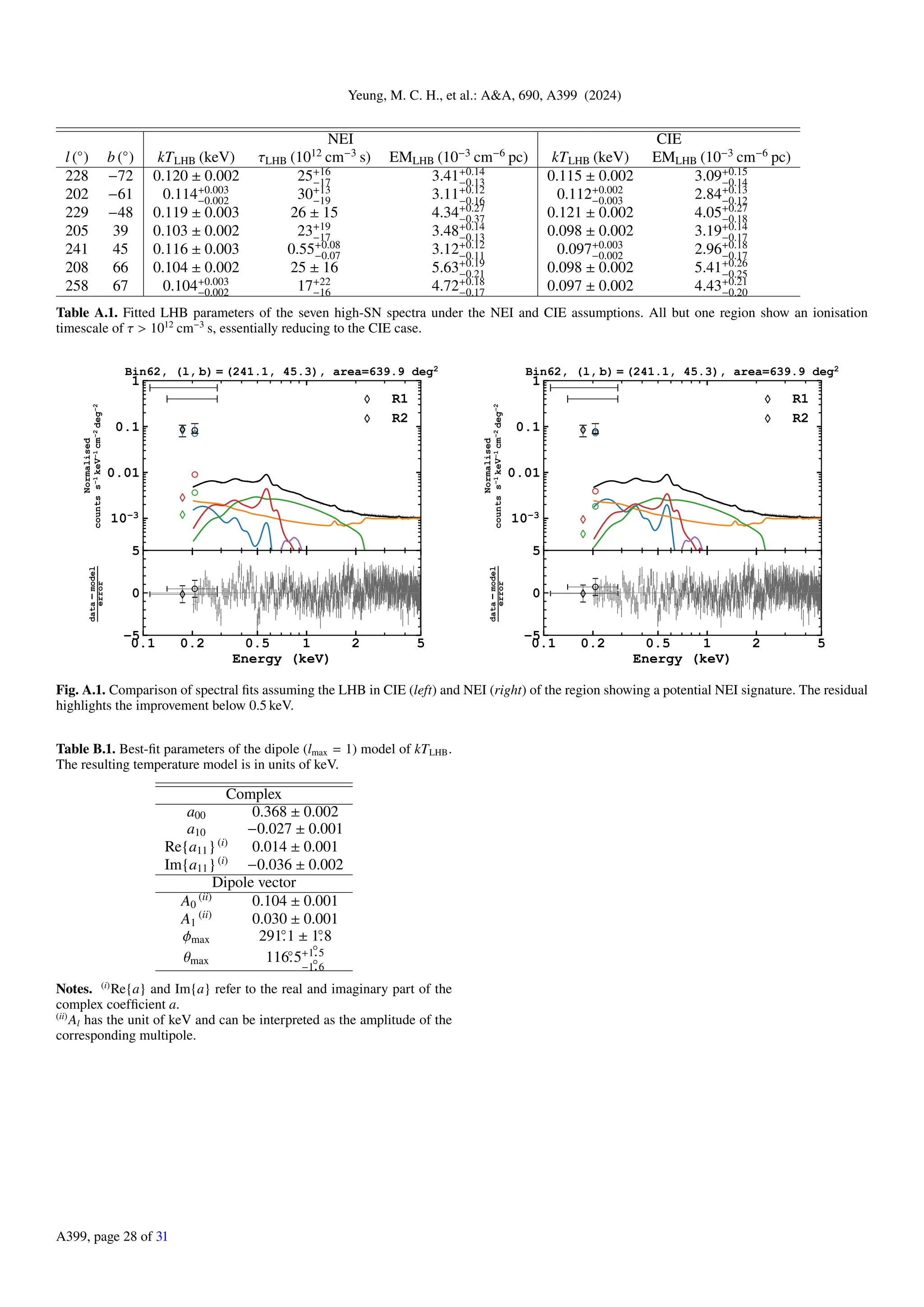
Download to read offline
![Yeung, M. C. H., et al.: A&A, 690, A399 (2024)
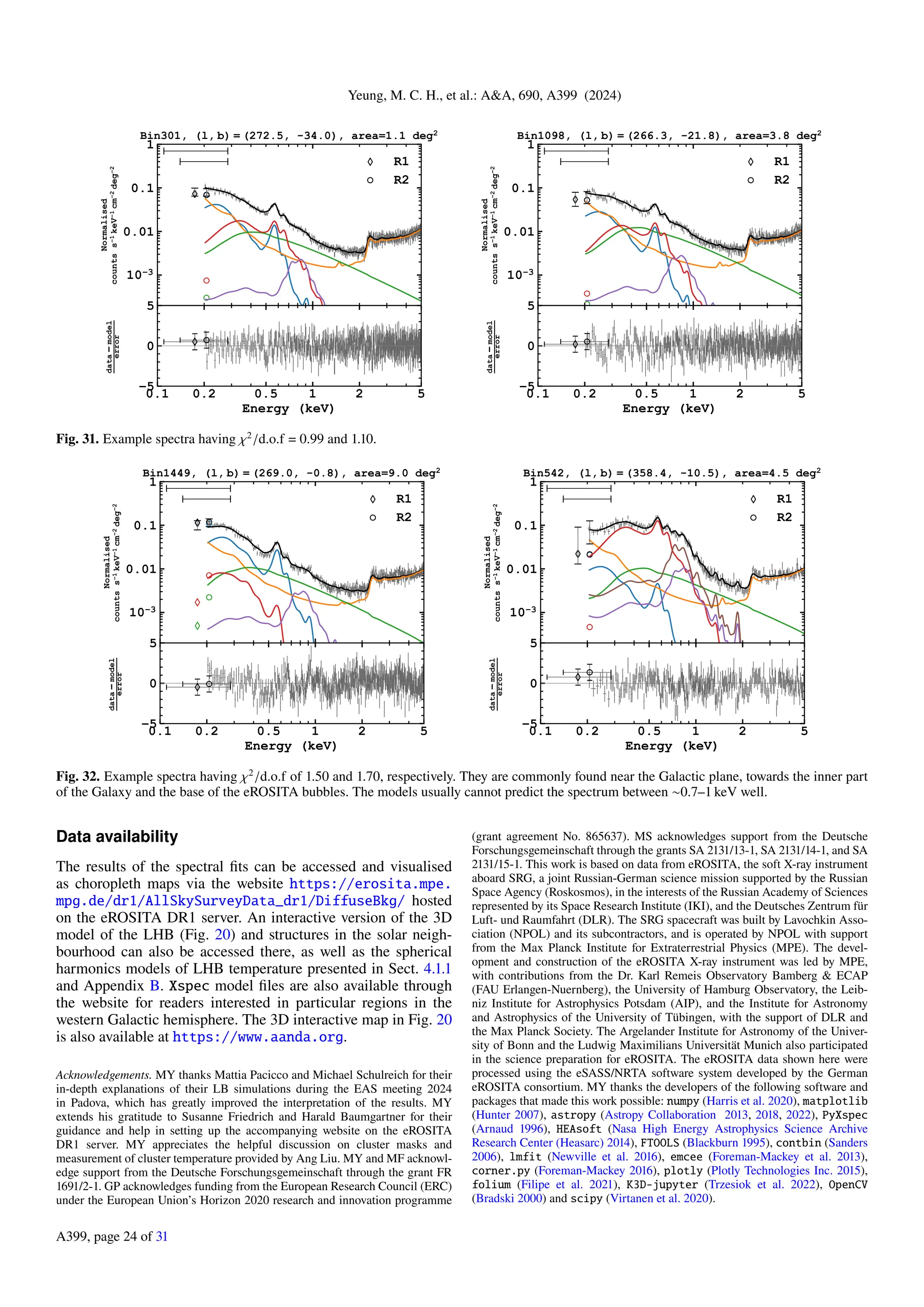
from a major micrometeoroid hit (Freyberg et al. 2022). We
rejected these sensitive pixels in addition. Last but not least, we
masked regions with overdense source detection (Merloni et al.
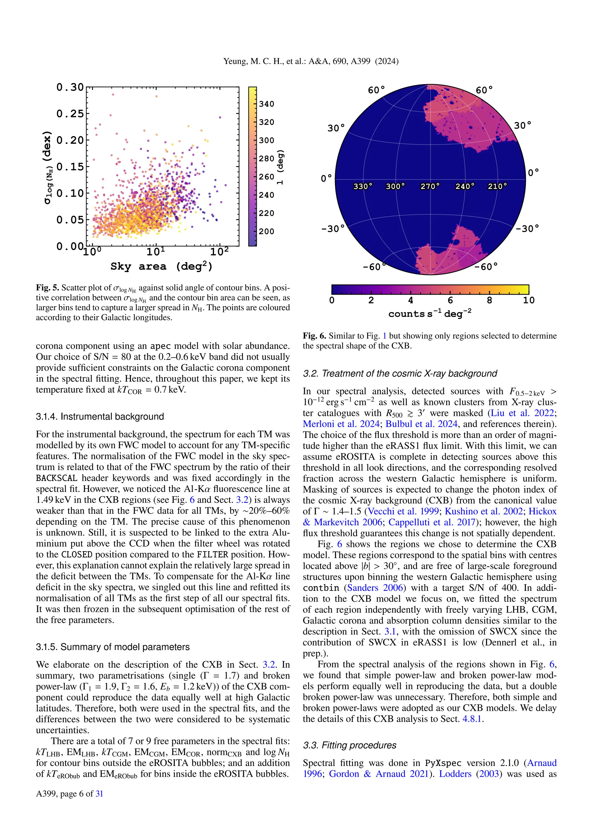
2024) and positions of known galaxy clusters with R500 ≳ 3′
as
described in Bulbul et al. (2024, and references therein). The
overdense source detection regions could be regions within or
near extended sources, such as supernova remnants or artefacts
caused by bright point sources, which triggered a high density of
spurious source detections.
Subsequently, we defined our spatial binning of spectral
extraction using the software contbin (Sanders 2006), with the
primary aim of dividing the western Galactic hemisphere into
bins of approximately constant S/N in the diffuse soft X-ray
emission, instead of imposing a regular grid system such as the
skytile system adopted by the standard products of eROSITA. For
our analysis, contbin also has the advantage of defining bins
with edges more closely following distinct features (for example,
from superbubbles, supernova remnants etc.) and being com-
putationally efficient compared to traditional Voronoi binning
codes. The binning was done on the eRASS1 0.2–0.6 keV dif-
fuse emission count map (all detected sources masked2
) after
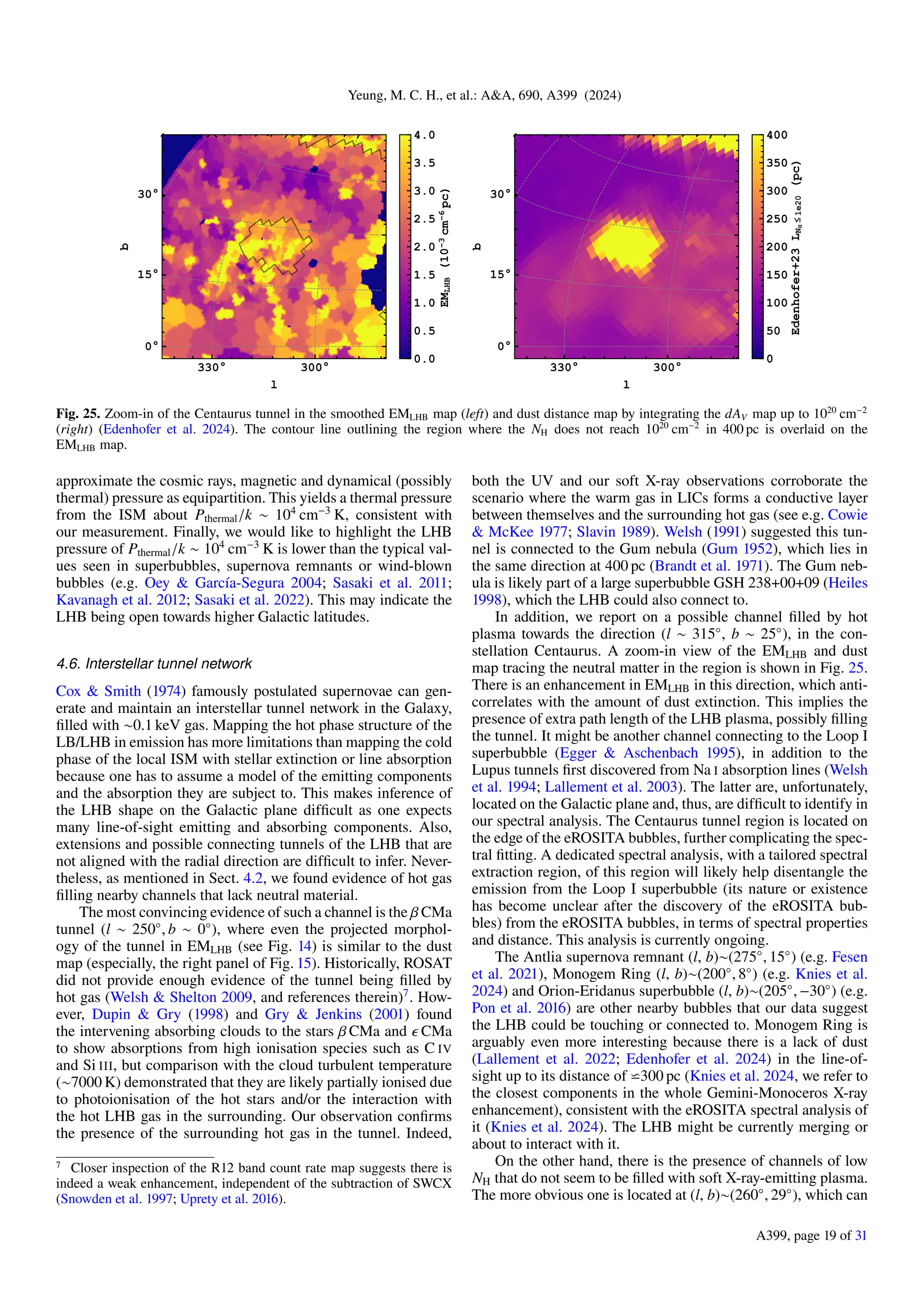
subtracting the expected counts from the non-X-ray background
measured from the filter-wheel-closed data (Yeung et al. 2023),
as this band contains the bulk of the emissions from the LHB
that eROSITA observes. This can be written explicitly as
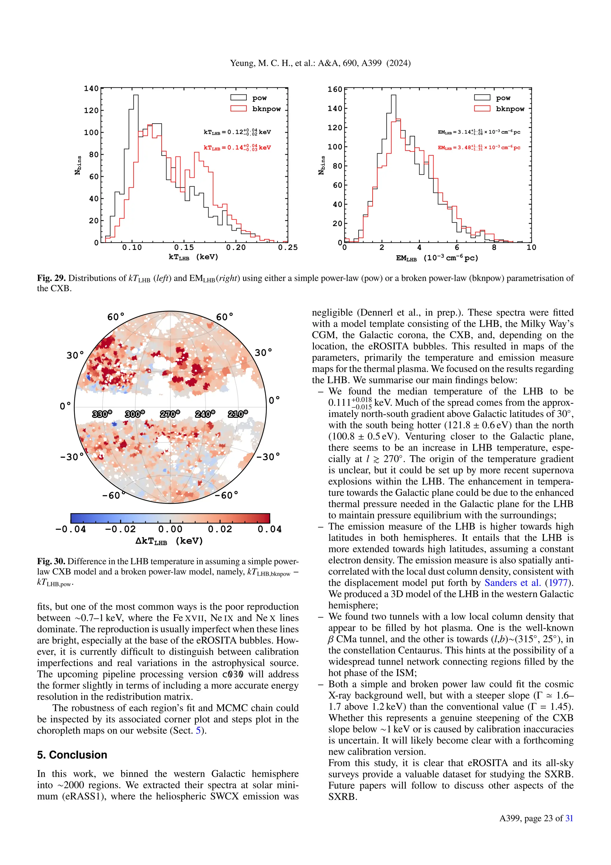
S (r) = C(r) − Bnonvig(r) (1)
= C(r) − Enonvig(r) × RFWC(r), (2)
where r, S , C and Bnonvig denote the sky position, signal, total
counts from diffuse emission, non-X-ray or non-vignetted back-
ground counts respectively. Bnonvig can be further written as a
product of non-vignetted exposure time (Enonvig) and the count
rate of the filter-wheel-closed background (RFWC). We estimate
the corresponding noise map N(r) for the S/N calculation using
equation (4) of Sanders (2006) as adopted from Gehrels (1986),
that is,
N(r) =
q
g[C(r)] + g[Bnonvig(r)] , (3)
where
g(c) = 1 +
r
c +
3
4
!2
(4)
is an estimation of the upper limit of the squared uncertainty
on c counts in Poissonian statistics. Before binning, the maps
were projected into the zenithal equal area (ZEA) projection.
Contour-binning yielded 2010 bins larger than 1 deg2
, which we
consider valid bins for spectral analysis. 1 deg2
is approximately
the eROSITA field-of-view. This selection primarily removed
areas near the south ecliptic pole and the Large Magellanic
Cloud where the exposure time is maximal due to the overlap-
ping of the scanning loci in eRASSs but are not representative of
the general SXRB.
2 More precisely, the masking of ‘all’ detected sources is done by
merging the CheeseMask images from the standard eSASS pipeline
from all the skytiles and project them into a HEALPix map of Nside =
4096 (pixel size ⋍51′′
) using nearest-neighbour interpolation. Con-
tribution from the masked pixels is then removed from the final
diffuse emission count map after downsampling the HEALPix map from
Nside = 4096 to Nside = 256.
0°
30°
60°
60°
30°
0°
-30°
-60° -60°
-30°
0 2 4 6 8 10
countss 1
deg 2
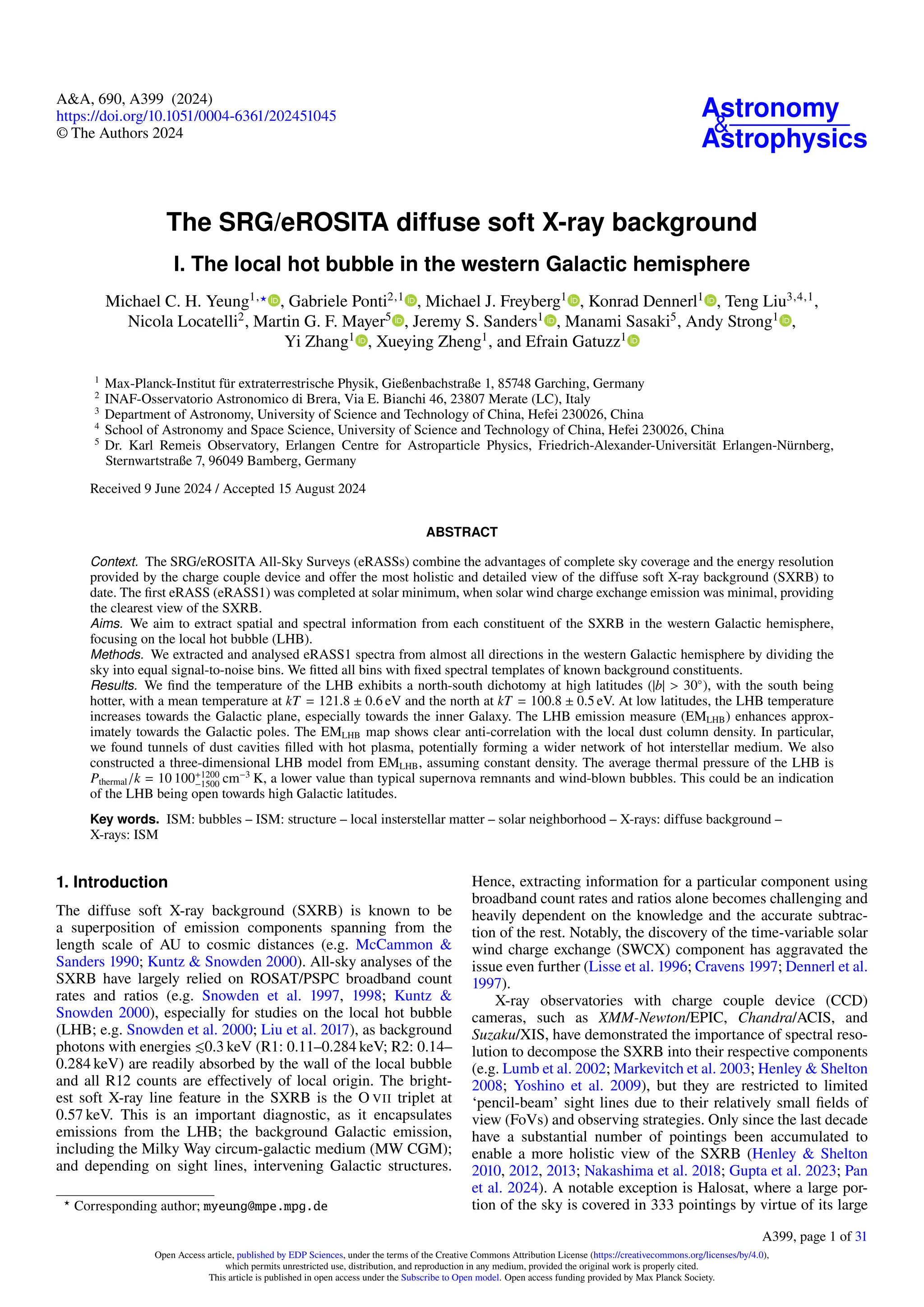
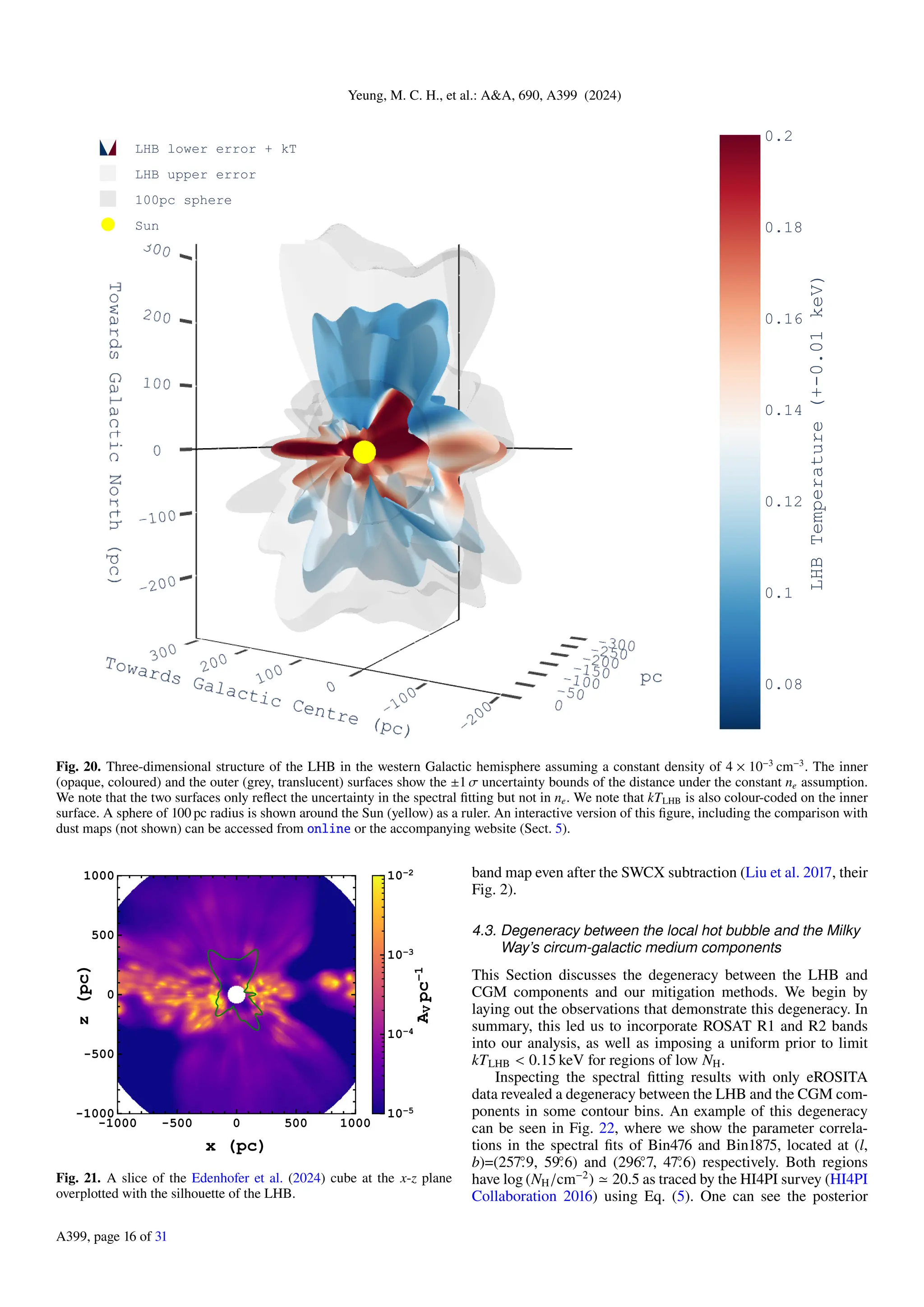
Fig. 1. Contour-binned eRASS1 0.2–0.6 keV band surface brightness
map in zenithal equal-area projection. Locations of big galaxy clusters,
overdense regions in source detection, and bins with sky area less than
1 deg2
were masked. Counts from the non-X-ray background and all
eRASS1-catalogued sources (Merloni et al. 2024) were also removed
from this image (but not in the spectra; see Sect. 2 for more details).
Fig. 2. Sky area distribution of the contour bins. It can be approximated
by a log-normal distribution, as shown with the red line.
Fig. 1 shows the contour-binned eRASS1 0.2–0.6 keV band
surface brightness map of the valid bins. Large soft X-ray emit-
ting structures such as the eROSITA bubbles (a pair of bubbles at
l ≳ 290◦
in the north and l ≳ 320◦
in the south), Antlia supernova
remnant (l, b)∼(275◦
, 15◦
), Monogem Ring (l, b)∼(200◦
, 8◦
) and
Orion-Eridanus Superbubble (l, b)∼(205◦
, −30◦
), and the Galac-
tic disc stand out in stark relief. The sky area distribution of the
valid contour bins is shown in Fig. 2. The median bin size is
∼7 deg2
. All bins with an area less than 1 deg2
were removed.
The distribution can be well approximated by a log-normal
function, as shown by the red line.
A399, page 3 of 31](https://image.slidesharecdn.com/aa51045-24-241228171219-95650a52/75/The-SRG-eROSITA-diffuse-soft-X-ray-background-3-2048.jpg)
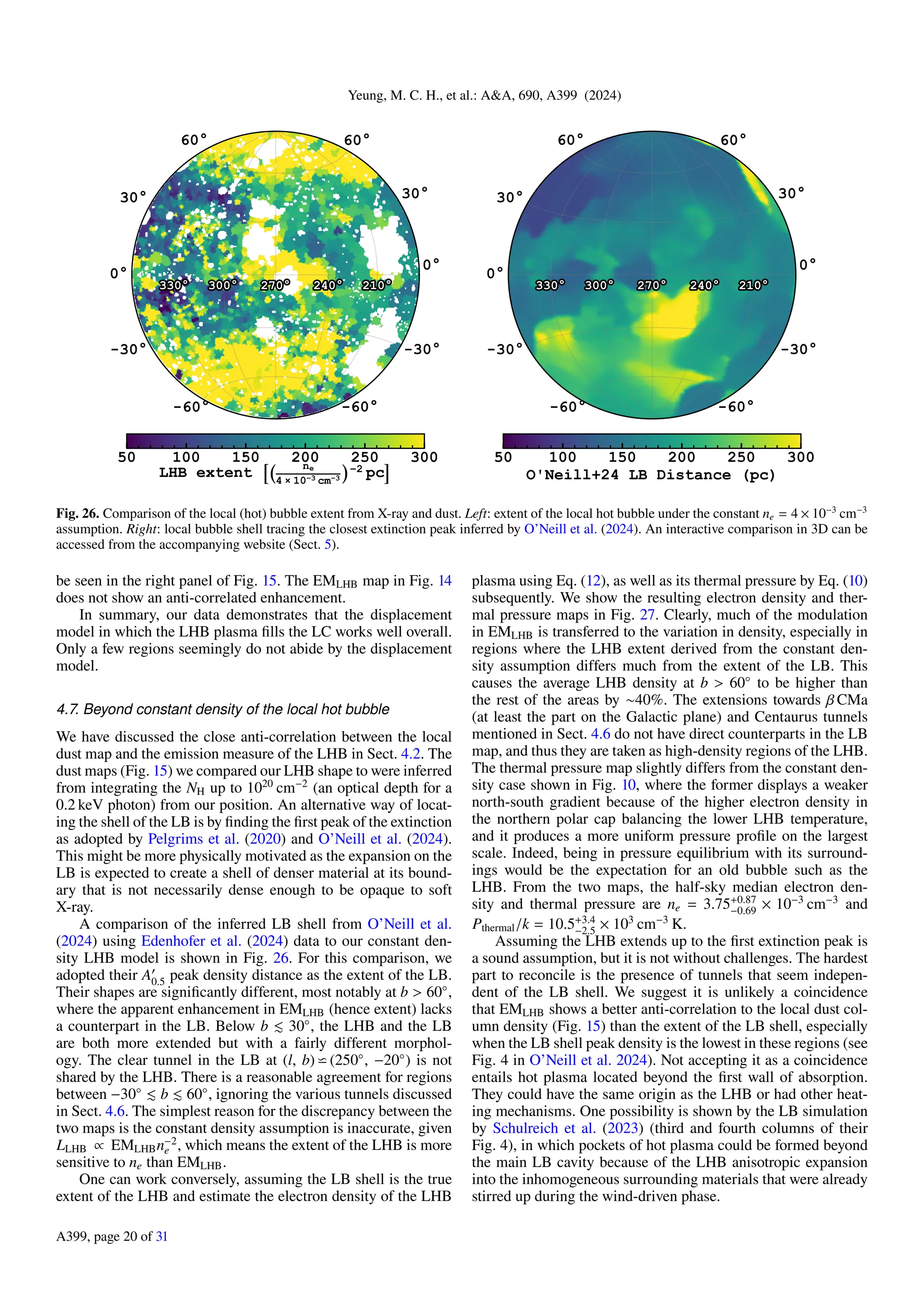
![Yeung, M. C. H., et al.: A&A, 690, A399 (2024)
Fig. 13. Comparison of our forward-modelled R2/R1 band ratio map with the observation. Left: R2/R1 band ratio map calculated by folding our
best-fit (median) spectral models with the ROSAT R1 and R2 band responses. Right: R2/R1 data binned to the same contour-binning scheme
(Snowden et al. 1997).
0°
30°
60°
60°
30°
0°
-30°
-60° -60°
-30°
100 200 300 400
LLHB [(
ne
4 × 10 3 cm 3 )
2 pc]
1 2 3 4 5
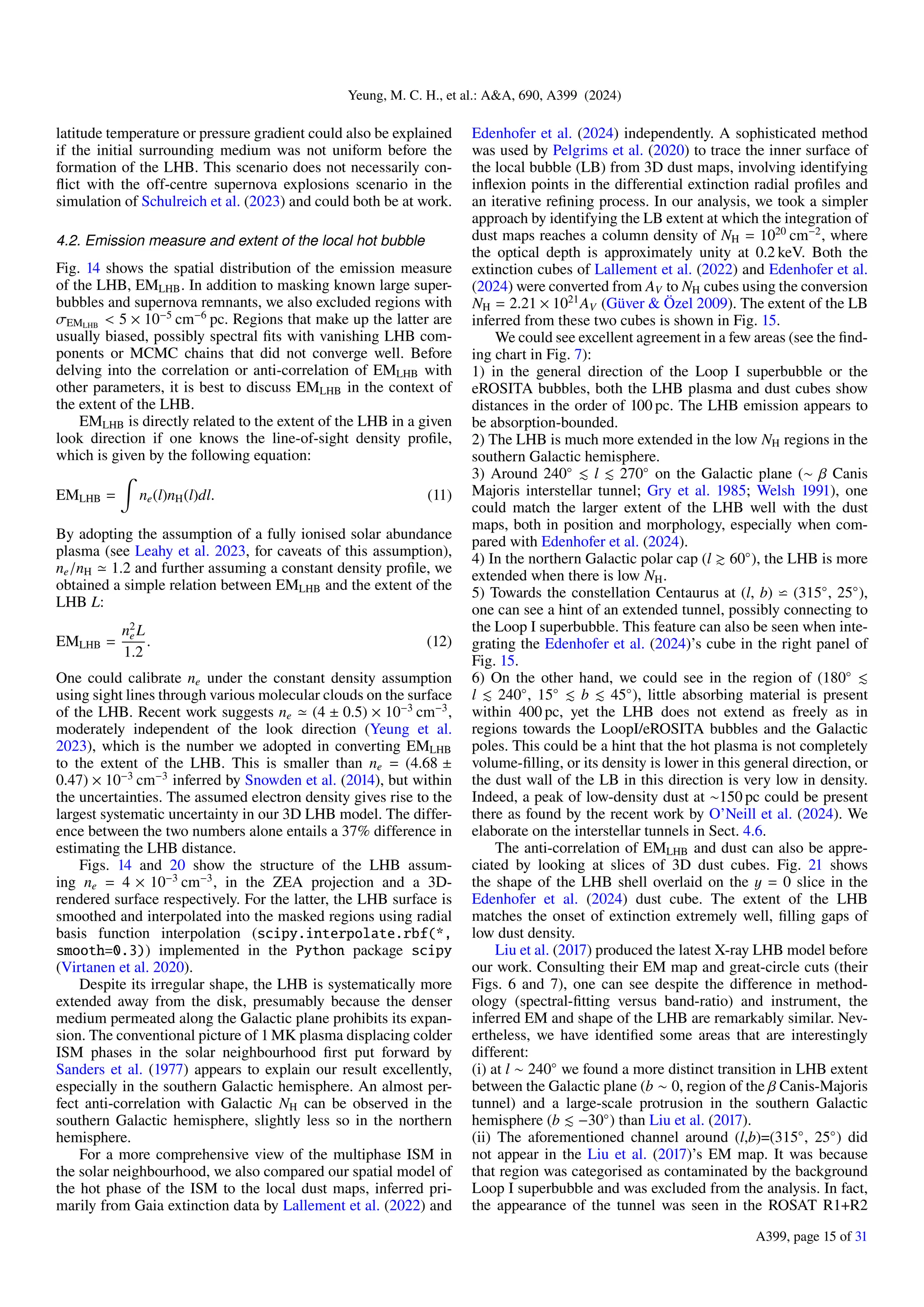
EMLHB(10 3 cm 6 pc)
Fig. 14. Spatial distribution of EMLHB. Regions with EMLHB uncertainty
< 5 × 10⁻⁵
cm−6
pc were also masked. The solid black line indicates
the position of the ecliptic, and the two dashed lines represent a range
of ±25◦
around it in ecliptic latitude where the solar wind density is
expected to be high. The extent of the LHB under the assumption of
ne = 4 × 10⁻³
cm−3
is also shown.
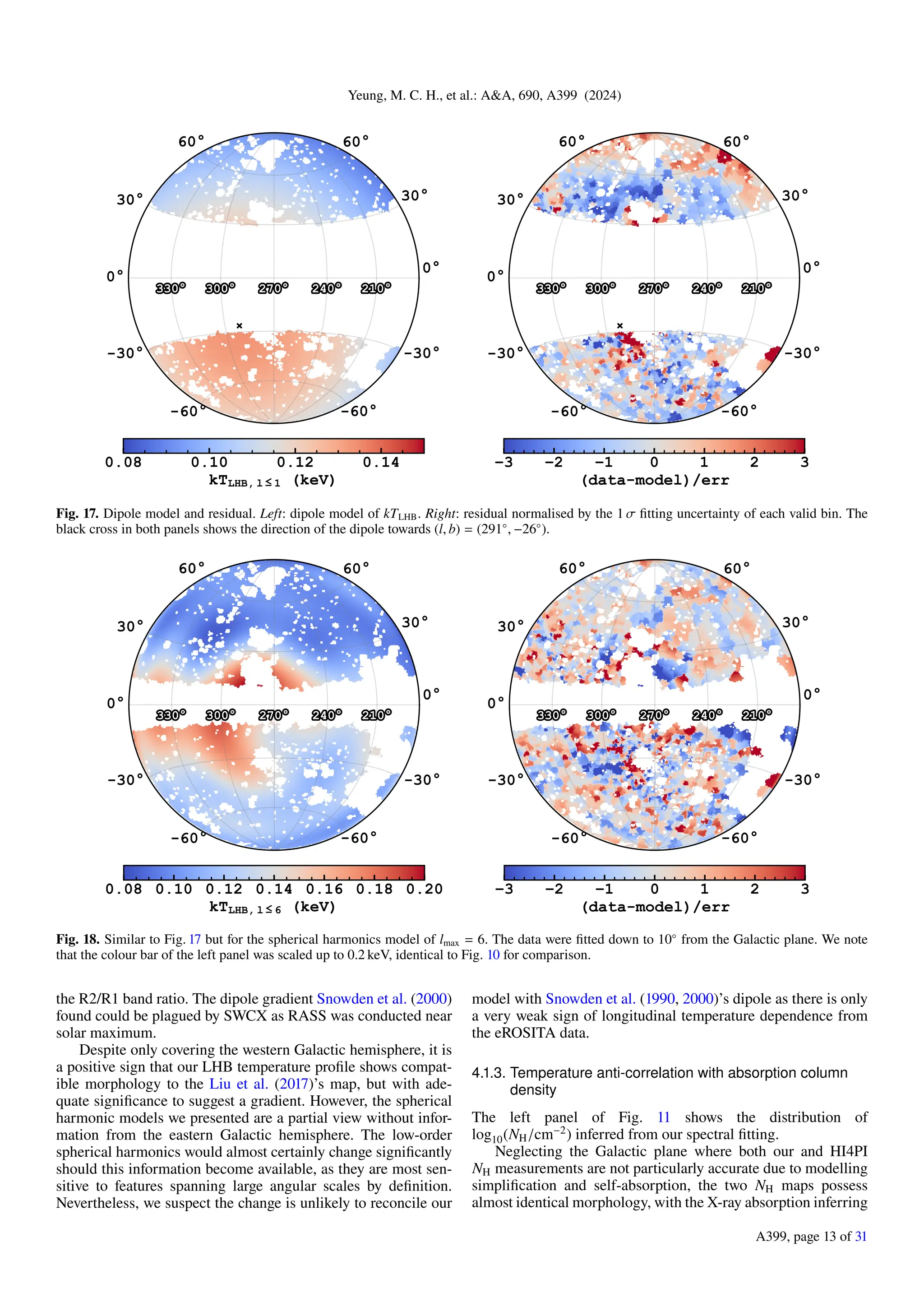
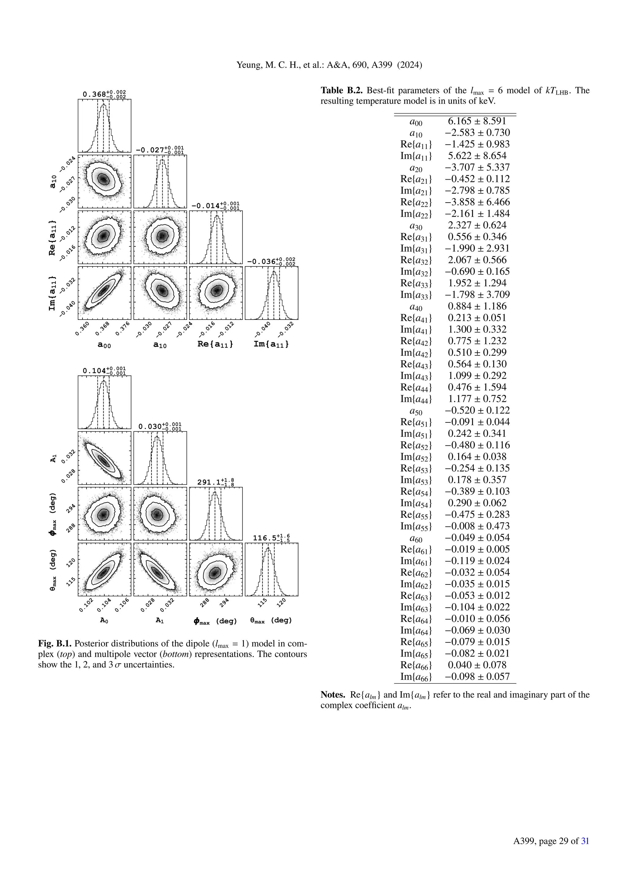
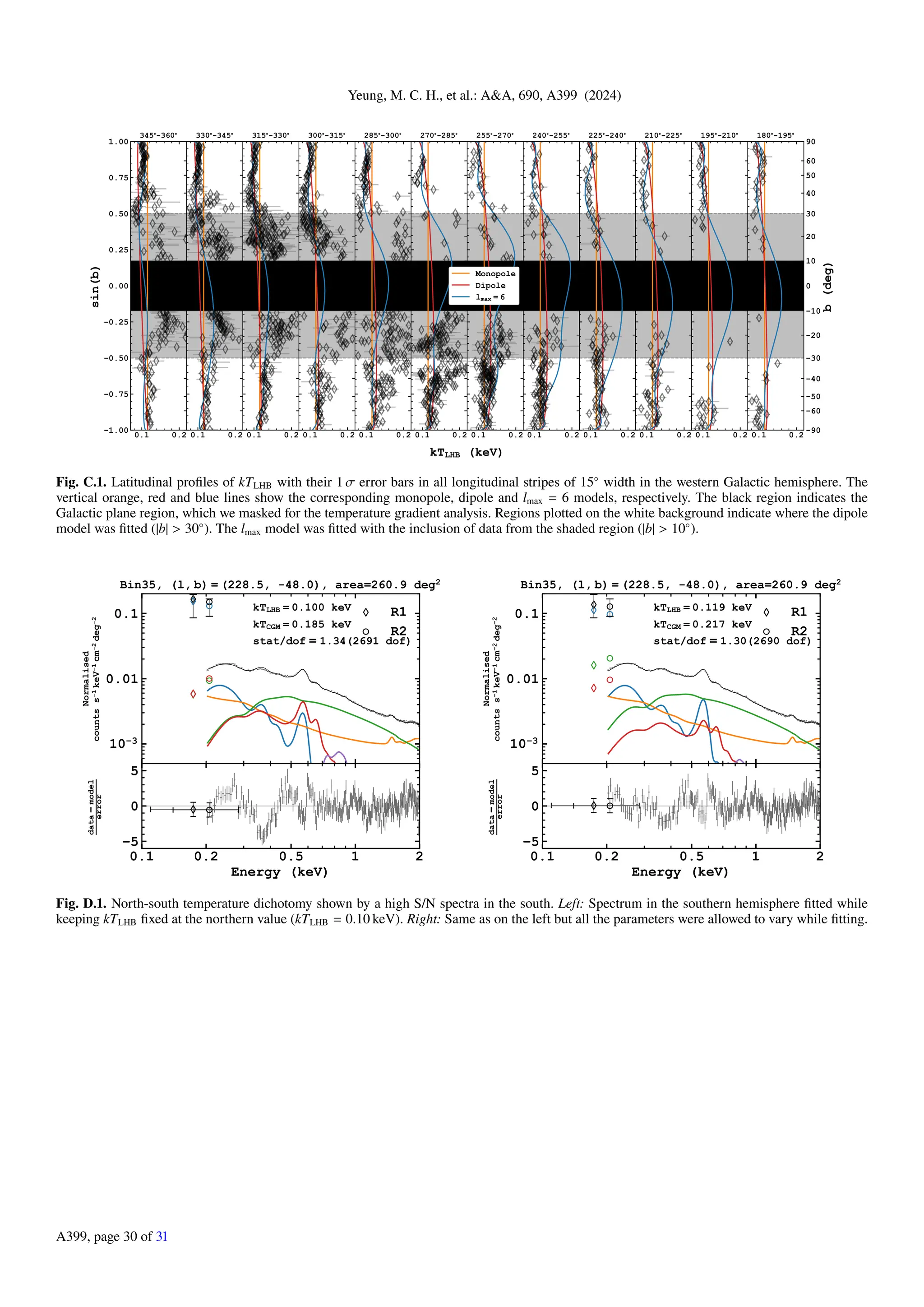
We began by modelling kTLHB as a constant (monopole) in
the unmasked regions. We found a median kTLHB of 0.1154 ±
0.0003 keV with χ2
/d.o.f = 6.36 (915 d.o.f), a unacceptable fit.
Subsequently, we fitted the data with a dipole (lmax ≤ 1). The
most probable model and the corresponding residual normalised
by the bins’ fitting uncertainty are shown in Fig. 17. The χ2
/d.o.f
decreased to 4.01 (912 d.o.f) compared to the monopole. Using
the F-test and a significance level of 0.001, we deduced an F-
statistic of 179.7 > Fcrit = 5.5 with a p-value in the order of
10−16
. This suggests the dipole model is strongly preferred over
the constant model, and the presence of a north-south gradient is
statistically significant. However, one could still recognise sys-
tematic residuals in the northern hemisphere by inspecting the
residual image, reflecting the north–south gradient is not simply
a dipole.
Naturally, raising lmax can improve the fidelity of our spher-
ical harmonics model to reproduce the data more closely. We
included data as close as 10◦
from the Galactic plane for this
empirical model. With multiple trials of different lmax values, we
arrived at a lmax = 6 model that captures the main large-scale
features in the data reasonably well, presented in Fig. 18. It has a
χ2
/d.o.f of 3.11 (1560 d.o.f.). We emphasise that we do not asso-
ciate any physical interpretations with the multipoles. It merely
serves as an empirical model for the LHB temperature profile.
However, we speculate on the origin of the gradient in Sect. 4.1.4.
The model parameters can be found in Appendix B. Appendix C
presents the latitudinal profiles of kTLHB, where both the uncer-
tainties and scatters of kTLHB are shown to compare with the
spherical harmonics models.
4.1.2. Comparison with past observations
The most relevant references on the large-scale temperature vari-
ations of the LHB are Snowden et al. (1990), Snowden et al.
(2000) and Liu et al. (2017). Snowden et al. (1990) inferred a
temperature gradient of the LHB for the first time using the
Wisconsin B/C band intensity ratio. They reported a mean tem-
perature of 0.097 keV (106.05
K), and a dipole gradient pointing
towards (l,b) = (348.
◦
7,−11.
◦
2) going from 0.064 keV (105.87
K;
near Galactic anti-centre) to 0.127 keV (106.17
K; near Galac-
tic centre). With the advent of ROSAT All-Sky Survey data
(RASS), Snowden et al. (2000) compiled a catalogue of X-
ray shadows at high Galactic latitudes (|b| > 20◦
). With these
A399, page 11 of 31](https://image.slidesharecdn.com/aa51045-24-241228171219-95650a52/75/The-SRG-eROSITA-diffuse-soft-X-ray-background-11-2048.jpg)
![Yeung, M. C. H., et al.: A&A, 690, A399 (2024)
References
Anders, E., & Grevesse, N. 1989, Geochim. Cosmochim. Acta, 53, 197
Arnaud, K. A. 1996, in Astronomical Data Analysis Software and Systems V, eds.
G. H. Jacoby, & J. Barnes, Astronomical Society of the Pacific Conference
Series, 101, 17
Astropy Collaboration (Robitaille, T. P., et al.) 2013, A&A, 558, A33
Astropy Collaboration (Price-Whelan, A. M., et al.) 2018, AJ, 156, 123
Astropy Collaboration (Price-Whelan, A. M., et al.) 2022, ApJ, 935, 167
Blackburn, J. K. 1995, in Astronomical Data Analysis Software and Systems IV,
eds. R. A. Shaw, H. E. Payne, & J. J. E. Hayes, Astronomical Society of the
Pacific Conference Series, 77, 367
Bluem, J., Kaaret, P., Kuntz, K. D., et al. 2022, ApJ, 936, 72
Bobin, J., Rapin, J., Larue, A., & Starck, J.-L. 2015, Trans. Sig. Proc., 63,
1199–1213
Boulares, A., & Cox, D. P. 1990, ApJ, 365, 544
Bradski, G. 2000, Dr. Dobb’s Journal of Software Tools
Brandt, J. C., Stecher, T. P., Crawford, D. L., & Maran, S. P. 1971, ApJ, 163, L99
Bregman, J. N., & Lloyd-Davies, E. J. 2007, ApJ, 669, 990
Breitschwerdt, D., & Schmutzler, T. 1994, Nature, 371, 774
Breitschwerdt, D., & de Avillez, M. A. 2021, Ap&SS, 366, 94
Bulbul, E., Liu, A., Kluge, M., et al. 2024, A&A, 685, A106
Burlaga, L. F., & Ness, N. F. 2014, ApJ, 784, 146
Cappelluti, N., Li, Y., Ricarte, A., et al. 2017, ApJ, 837, 19
Carloni Gertosio, R., Bobin, J., & Acero, F. 2023, Signal Process., 202, 108776
Cash, W. 1979, ApJ, 228, 939
Cowie, L. L., & McKee, C. F. 1977, ApJ, 211, 135
Cox, D. P. 2005, ARA&A, 43, 337
Cox, D. P., & Smith, B. W. 1974, ApJ, 189, L105
Cravens, T. E. 1997, Geophys. Res. Lett., 24, 105
Crowder, S. G., Barger, K. A., Brandl, D. E., et al. 2012, ApJ, 758, 143
Das, S., Mathur, S., Nicastro, F., & Krongold, Y. 2019, ApJ, 882, L23
de Avillez, M. A., & Breitschwerdt, D. 2012, A&A, 539, L1
De Luca, A., & Molendi, S. 2004, A&A, 419, 837
Dennerl, K. 2010, Space Sci. Rev., 157, 57
Dennerl, K., Englhauser, J., & Trümper, J. 1997, Science, 277, 1625
Dupin, O., & Gry, C. 1998, A&A, 335, 661
Edenhofer, G., Zucker, C., Frank, P., et al. 2024, A&A, 685, A82
Egger, R. J., & Aschenbach, B. 1995, A&A, 294, L25
Fang, T., & Jiang, X. 2014, ApJ, 785, L24
Fang, T., Buote, D., Bullock, J., & Ma, R. 2015, ApJS, 217, 21
Fesen, R. A., Drechsler, M., Weil, K. E., et al. 2021, ApJ, 920, 90
Filipe, Journois, M., Frank, et al. 2021, https://doi.org/10.5281/zenodo.
4447642
Foreman-Mackey, D. 2016, corner.py: Scatterplot matrices in Python
Foreman-Mackey, D., Hogg, D. W., Lang, D., & Goodman, J. 2013, PASP, 125,
306
Foster, A. R., Ji, L., Smith, R. K., & Brickhouse, N. S. 2012, ApJ, 756, 128
Freyberg, M., Perinati, E., Pacaud, F., et al. 2020, SPIE Conf. Ser., 11444,
114441O
Freyberg, M. J., Müller, T., Perinati, E., et al. 2022, SPIE Conf. Ser., 12181,
1218155
Frisch, P. C., Redfield, S., & Slavin, J. D. 2011, ARA&A, 49, 237
Fuchs, B., Breitschwerdt, D., de Avillez, M. A., Dettbarn, C., & Flynn, C. 2006,
MNRAS, 373, 993
Galeazzi, M., Gupta, A., Covey, K., & Ursino, E. 2007, ApJ, 658, 1081
Galeazzi, M., Collier, M. R., Cravens, T., et al. 2012, Astron. Nachr., 333, 383
Gehrels, N. 1986, ApJ, 303, 336
Gilli, R., Comastri, A., & Hasinger, G. 2007, A&A, 463, 79
Goodman, J., & Weare, J. 2010, Commun. Appl. Math. Computat. Sci., 5, 65
Gordon, C., & Arnaud, K. 2021, PyXspec: Python interface to XSPEC
spectral-fitting program, Astrophysics Source Code Library [record
ascl:2101.014]
Gry, C., & Jenkins, E. B. 2001, A&A, 367, 617
Gry, C., York, D. G., & Vidal-Madjar, A. 1985, ApJ, 296, 593
Gu, L., Mao, J., Costantini, E., & Kaastra, J. 2016, A&A, 594, A78
Gum, C. S. 1952, The Observatory, 72, 151
Gupta, A., Kingsbury, J., Mathur, S., et al. 2021, ApJ, 909, 164
Gupta, A., Mathur, S., Kingsbury, J., Das, S., & Krongold, Y. 2023, Nat. Astron.,
7, 799
Güver, T., & Özel, F. 2009, MNRAS, 400, 2050
Harris, C. R., Millman, K. J., van der Walt, S. J., et al. 2020, Nature, 585, 357
Hasinger, G., Burg, R., Giacconi, R., et al. 1993, A&A, 275, 1
Heiles, C. 1998, ApJ, 498, 689
Henley, D. B., & Shelton, R. L. 2008, ApJ, 676, 335
Henley, D. B., & Shelton, R. L. 2010, ApJS, 187, 388
Henley, D. B., & Shelton, R. L. 2012, ApJS, 202, 14
Henley, D. B., & Shelton, R. L. 2013, ApJ, 773, 92
Henley, D. B., Shelton, R. L., & Kuntz, K. D. 2007, ApJ, 661, 304
HI4PI Collaboration (Ben Bekhti, N., et al.) 2016, A&A, 594, A116
Hickox, R. C., & Markevitch, M. 2006, ApJ, 645, 95
Hunter, J. D. 2007, Comput. Sci. Eng., 9, 90
Kaaret, P., Zajczyk, A., LaRocca, D. M., et al. 2019, ApJ, 884, 162
Kaaret, P., Koutroumpa, D., Kuntz, K. D., et al. 2020, Nat. Astron., 4, 1072
Kaastra, J. S. 2017, A&A, 605, A51
Kaastra, J. S., & Bleeker, J. A. M. 2016, A&A, 587, A151
Kameda, S., Ikezawa, S., Sato, M., et al. 2017, Geophys. Res. Lett., 44, 11,706
Kataoka, J., Tahara, M., Totani, T., et al. 2013, ApJ, 779, 57
Kavanagh, P. J., Sasaki, M., & Points, S. D. 2012, A&A, 547, A19
Knies, J. R., Sasaki, M., Becker, W., et al. 2024, A&A, 688, A90
Kuntz, K. D. 2019, A&A Rev., 27, 1
Kuntz, K. D., & Snowden, S. L. 2000, ApJ, 543, 195
Kushino, A., Ishisaki, Y., Morita, U., et al. 2002, PASJ, 54, 327
Lallement, R., Welsh, B. Y., Vergely, J. L., Crifo, F., & Sfeir, D. 2003, A&A,
411, 447
Lallement, R., Snowden, S., Kuntz, K. D., et al. 2016, A&A, 595, A131
Lallement, R., Vergely, J. L., Babusiaux, C., & Cox, N. L. J. 2022, A&A, 661,
A147
Leahy, D., Foster, A., & Seitenzahl, I. 2023, arXiv e-prints [arXiv:2311.11181]
Liedahl, D. A., Osterheld, A. L., & Goldstein, W. H. 1995, ApJ, 438, L115
Lisse, C. M., Dennerl, K., Englhauser, J., et al. 1996, Science, 274, 205
Liu, W., Chiao, M., Collier, M. R., et al. 2017, ApJ, 834, 33
Liu, A., Bulbul, E., Ghirardini, V., et al. 2022, A&A, 661, A2
Liu, A., Bulbul, E., Ramos-Ceja, M. E., et al. 2023, A&A, 670, A96
Locatelli, N., Ponti, G., & Bianchi, S. 2022, A&A, 659, A118
Locatelli, N., Ponti, G., Merloni, A., et al. 2024, A&A, 688, A85
Lodders, K. 2003, ApJ, 591, 1220
Lumb, D. H., Warwick, R. S., Page, M., & De Luca, A. 2002, A&A, 389,
93
Luo, B., Brandt, W. N., Xue, Y. Q., et al. 2017, ApJS, 228, 2
Markevitch, M., Bautz, M. W., Biller, B., et al. 2003, ApJ, 583, 70
McCammon, D., & Sanders, W. T. 1990, ARA&A, 28, 657
McCammon, D., Almy, R., Apodaca, E., et al. 2002, ApJ, 576, 188
McComas, D. J., Bame, S. J., Barraclough, B. L., et al. 1998, Geophys. Res. Lett.,
25, 1
McComas, D. J., Elliott, H. A., Schwadron, N. A., et al. 2003, Geo-
phys. Res. Lett., 30, 1517
Merloni, A., Lamer, G., Liu, T., et al. 2024, A&A, 682, A34
Mewe, R., Gronenschild, E. H. B. M., & van den Oord, G. H. J. 1985, A&AS,
62, 197
Mewe, R., Lemen, J. R., & van den Oord, G. H. J. 1986, A&AS, 65, 511
Migkas, K., Kox, D., Schellenberger, G., et al. 2024, A&A, 688, A107
Miller, M. J., & Bregman, J. N. 2013, ApJ, 770, 118
Miller, M. J., & Bregman, J. N. 2015, ApJ, 800, 14
Miller, E. D., Tsunemi Hiroshi, Bautz, M. W., et al. 2008, PASJ, 60, S95
Mou, G., Sun, D., Fang, T., et al. 2023, Nat. Commun., 14, 781
Nakashima, S., Inoue, Y., Yamasaki, N., et al. 2018, ApJ, 862, 34
Nasa High Energy Astrophysics Science Archive Research Center (Heasarc).
2014, HEAsoft: Unified Release of FTOOLS and XANADU
Newville, M., Stensitzki, T., Allen, D. B., et al. 2016, Lmfit: Non-Linear Least-
Square Minimization and Curve-Fitting for Python, Astrophysics Source
Code Library [record ascl:1606.014]
Oey, M. S., & García-Segura, G. 2004, ApJ, 613, 302
O’Neill, T. J., Zucker, C., Goodman, A. A., & Edenhofer, G. 2024, ApJ, 973, 136
Pan, Z., Qu, Z., Bregman, J. N., & Liu, J. 2024, ApJS, 271, 62
Pelgrims, V., Ferrière, K., Boulanger, F., Lallement, R., & Montier, L. 2020,
A&A, 636, A17
Picquenot, A., Acero, F., Bobin, J., et al. 2019, A&A, 627, A139
Picquenot, A., Acero, F., Holland-Ashford, T., Lopez, L. A., & Bobin, J. 2021,
A&A, 646, A82
Picquenot, A., Williams, B. J., Acero, F., & Guest, B. T. 2023, A&A, 672, A57
Planck Collaboration XI. 2014, A&A, 571, A11
Plotly Technologies Inc. 2015, Collaborative data science
Pon, A., Ochsendorf, B. B., Alves, J., et al. 2016, ApJ, 827, 42
Ponti, G., Zheng, X., Locatelli, N., et al. 2023, A&A, 674, A195
Porowski, C., Bzowski, M., & Tokumaru, M. 2022, ApJS, 259, 2
Predehl, P., Sunyaev, R. A., Becker, W., et al. 2020, Nature, 588, 227
Predehl, P., Andritschke, R., Arefiev, V., et al. 2021, A&A, 647, A1
Putman, M. E., Peek, J. E. G., & Joung, M. R. 2012, ARA&A, 50, 491
Qu, Z., Koutroumpa, D., Bregman, J. N., Kuntz, K. D., & Kaaret, P. 2022, ApJ,
930, 21
Raymond, J. C., & Smith, B. W. 1977, ApJS, 35, 419
Ringuette, R., Koutroumpa, D., Kuntz, K. D., et al. 2021, ApJ, 918, 41
Sakai, K., Mitsuda, K., Yamasaki, N. Y., et al. 2012, in Suzaku 2011: Explor-
ing the X-ray Universe: Suzaku and Beyond, eds. R. Petre, K. Mitsuda, &
L. Angelini, American Institute of Physics Conference Series, 1427, 342
A399, page 25 of 31](https://image.slidesharecdn.com/aa51045-24-241228171219-95650a52/75/The-SRG-eROSITA-diffuse-soft-X-ray-background-25-2048.jpg)


![Yeung, M. C. H., et al.: A&A, 690, A399 (2024)
from a major micrometeoroid hit (Freyberg et al. 2022). We
rejected these sensitive pixels in addition. Last but not least, we
masked regions with overdense source detection (Merloni et al.
2024) and positions of known galaxy clusters with R500 ≳ 3′
as
described in Bulbul et al. (2024, and references therein). The
overdense source detection regions could be regions within or
near extended sources, such as supernova remnants or artefacts
caused by bright point sources, which triggered a high density of
spurious source detections.
Subsequently, we defined our spatial binning of spectral
extraction using the software contbin (Sanders 2006), with the
primary aim of dividing the western Galactic hemisphere into
bins of approximately constant S/N in the diffuse soft X-ray
emission, instead of imposing a regular grid system such as the
skytile system adopted by the standard products of eROSITA. For
our analysis, contbin also has the advantage of defining bins
with edges more closely following distinct features (for example,
from superbubbles, supernova remnants etc.) and being com-
putationally efficient compared to traditional Voronoi binning
codes. The binning was done on the eRASS1 0.2–0.6 keV dif-
fuse emission count map (all detected sources masked2
) after
subtracting the expected counts from the non-X-ray background
measured from the filter-wheel-closed data (Yeung et al. 2023),
as this band contains the bulk of the emissions from the LHB
that eROSITA observes. This can be written explicitly as
S (r) = C(r) − Bnonvig(r) (1)
= C(r) − Enonvig(r) × RFWC(r), (2)
where r, S , C and Bnonvig denote the sky position, signal, total
counts from diffuse emission, non-X-ray or non-vignetted back-
ground counts respectively. Bnonvig can be further written as a
product of non-vignetted exposure time (Enonvig) and the count
rate of the filter-wheel-closed background (RFWC). We estimate
the corresponding noise map N(r) for the S/N calculation using
equation (4) of Sanders (2006) as adopted from Gehrels (1986),
that is,
N(r) =
q
g[C(r)] + g[Bnonvig(r)] , (3)
where
g(c) = 1 +
r
c +
3
4
!2
(4)
is an estimation of the upper limit of the squared uncertainty
on c counts in Poissonian statistics. Before binning, the maps
were projected into the zenithal equal area (ZEA) projection.
Contour-binning yielded 2010 bins larger than 1 deg2
, which we
consider valid bins for spectral analysis. 1 deg2
is approximately
the eROSITA field-of-view. This selection primarily removed
areas near the south ecliptic pole and the Large Magellanic
Cloud where the exposure time is maximal due to the overlap-
ping of the scanning loci in eRASSs but are not representative of
the general SXRB.
2 More precisely, the masking of ‘all’ detected sources is done by
merging the CheeseMask images from the standard eSASS pipeline
from all the skytiles and project them into a HEALPix map of Nside =
4096 (pixel size ⋍51′′
) using nearest-neighbour interpolation. Con-
tribution from the masked pixels is then removed from the final
diffuse emission count map after downsampling the HEALPix map from
Nside = 4096 to Nside = 256.
0°
30°
60°
60°
30°
0°
-30°
-60° -60°
-30°
0 2 4 6 8 10
countss 1
deg 2
Fig. 1. Contour-binned eRASS1 0.2–0.6 keV band surface brightness
map in zenithal equal-area projection. Locations of big galaxy clusters,
overdense regions in source detection, and bins with sky area less than
1 deg2
were masked. Counts from the non-X-ray background and all
eRASS1-catalogued sources (Merloni et al. 2024) were also removed
from this image (but not in the spectra; see Sect. 2 for more details).
Fig. 2. Sky area distribution of the contour bins. It can be approximated
by a log-normal distribution, as shown with the red line.
Fig. 1 shows the contour-binned eRASS1 0.2–0.6 keV band
surface brightness map of the valid bins. Large soft X-ray emit-
ting structures such as the eROSITA bubbles (a pair of bubbles at
l ≳ 290◦
in the north and l ≳ 320◦
in the south), Antlia supernova
remnant (l, b)∼(275◦
, 15◦
), Monogem Ring (l, b)∼(200◦
, 8◦
) and
Orion-Eridanus Superbubble (l, b)∼(205◦
, −30◦
), and the Galac-
tic disc stand out in stark relief. The sky area distribution of the
valid contour bins is shown in Fig. 2. The median bin size is
∼7 deg2
. All bins with an area less than 1 deg2
were removed.
The distribution can be well approximated by a log-normal
function, as shown by the red line.
A399, page 3 of 31](https://crownmelresort.com/image.slidesharecdn.com/aa51045-24-241228171219-95650a52/75/The-SRG-eROSITA-diffuse-soft-X-ray-background-3-2048.jpg)


![Yeung, M. C. H., et al.: A&A, 690, A399 (2024)
Fig. 13. Comparison of our forward-modelled R2/R1 band ratio map with the observation. Left: R2/R1 band ratio map calculated by folding our
best-fit (median) spectral models with the ROSAT R1 and R2 band responses. Right: R2/R1 data binned to the same contour-binning scheme
(Snowden et al. 1997).
0°
30°
60°
60°
30°
0°
-30°
-60° -60°
-30°
100 200 300 400
LLHB [(
ne
4 × 10 3 cm 3 )
2 pc]
1 2 3 4 5
EMLHB(10 3 cm 6 pc)
Fig. 14. Spatial distribution of EMLHB. Regions with EMLHB uncertainty
< 5 × 10⁻⁵
cm−6
pc were also masked. The solid black line indicates
the position of the ecliptic, and the two dashed lines represent a range
of ±25◦
around it in ecliptic latitude where the solar wind density is
expected to be high. The extent of the LHB under the assumption of
ne = 4 × 10⁻³
cm−3
is also shown.
We began by modelling kTLHB as a constant (monopole) in
the unmasked regions. We found a median kTLHB of 0.1154 ±
0.0003 keV with χ2
/d.o.f = 6.36 (915 d.o.f), a unacceptable fit.
Subsequently, we fitted the data with a dipole (lmax ≤ 1). The
most probable model and the corresponding residual normalised
by the bins’ fitting uncertainty are shown in Fig. 17. The χ2
/d.o.f
decreased to 4.01 (912 d.o.f) compared to the monopole. Using
the F-test and a significance level of 0.001, we deduced an F-
statistic of 179.7 > Fcrit = 5.5 with a p-value in the order of
10−16
. This suggests the dipole model is strongly preferred over
the constant model, and the presence of a north-south gradient is
statistically significant. However, one could still recognise sys-
tematic residuals in the northern hemisphere by inspecting the
residual image, reflecting the north–south gradient is not simply
a dipole.
Naturally, raising lmax can improve the fidelity of our spher-
ical harmonics model to reproduce the data more closely. We
included data as close as 10◦
from the Galactic plane for this
empirical model. With multiple trials of different lmax values, we
arrived at a lmax = 6 model that captures the main large-scale
features in the data reasonably well, presented in Fig. 18. It has a
χ2
/d.o.f of 3.11 (1560 d.o.f.). We emphasise that we do not asso-
ciate any physical interpretations with the multipoles. It merely
serves as an empirical model for the LHB temperature profile.
However, we speculate on the origin of the gradient in Sect. 4.1.4.
The model parameters can be found in Appendix B. Appendix C
presents the latitudinal profiles of kTLHB, where both the uncer-
tainties and scatters of kTLHB are shown to compare with the
spherical harmonics models.
4.1.2. Comparison with past observations
The most relevant references on the large-scale temperature vari-
ations of the LHB are Snowden et al. (1990), Snowden et al.
(2000) and Liu et al. (2017). Snowden et al. (1990) inferred a
temperature gradient of the LHB for the first time using the
Wisconsin B/C band intensity ratio. They reported a mean tem-
perature of 0.097 keV (106.05
K), and a dipole gradient pointing
towards (l,b) = (348.
◦
7,−11.
◦
2) going from 0.064 keV (105.87
K;
near Galactic anti-centre) to 0.127 keV (106.17
K; near Galac-
tic centre). With the advent of ROSAT All-Sky Survey data
(RASS), Snowden et al. (2000) compiled a catalogue of X-
ray shadows at high Galactic latitudes (|b| > 20◦
). With these
A399, page 11 of 31](https://crownmelresort.com/image.slidesharecdn.com/aa51045-24-241228171219-95650a52/75/The-SRG-eROSITA-diffuse-soft-X-ray-background-11-2048.jpg)


![Yeung, M. C. H., et al.: A&A, 690, A399 (2024)
References
Anders, E., & Grevesse, N. 1989, Geochim. Cosmochim. Acta, 53, 197
Arnaud, K. A. 1996, in Astronomical Data Analysis Software and Systems V, eds.
G. H. Jacoby, & J. Barnes, Astronomical Society of the Pacific Conference
Series, 101, 17
Astropy Collaboration (Robitaille, T. P., et al.) 2013, A&A, 558, A33
Astropy Collaboration (Price-Whelan, A. M., et al.) 2018, AJ, 156, 123
Astropy Collaboration (Price-Whelan, A. M., et al.) 2022, ApJ, 935, 167
Blackburn, J. K. 1995, in Astronomical Data Analysis Software and Systems IV,
eds. R. A. Shaw, H. E. Payne, & J. J. E. Hayes, Astronomical Society of the
Pacific Conference Series, 77, 367
Bluem, J., Kaaret, P., Kuntz, K. D., et al. 2022, ApJ, 936, 72
Bobin, J., Rapin, J., Larue, A., & Starck, J.-L. 2015, Trans. Sig. Proc., 63,
1199–1213
Boulares, A., & Cox, D. P. 1990, ApJ, 365, 544
Bradski, G. 2000, Dr. Dobb’s Journal of Software Tools
Brandt, J. C., Stecher, T. P., Crawford, D. L., & Maran, S. P. 1971, ApJ, 163, L99
Bregman, J. N., & Lloyd-Davies, E. J. 2007, ApJ, 669, 990
Breitschwerdt, D., & Schmutzler, T. 1994, Nature, 371, 774
Breitschwerdt, D., & de Avillez, M. A. 2021, Ap&SS, 366, 94
Bulbul, E., Liu, A., Kluge, M., et al. 2024, A&A, 685, A106
Burlaga, L. F., & Ness, N. F. 2014, ApJ, 784, 146
Cappelluti, N., Li, Y., Ricarte, A., et al. 2017, ApJ, 837, 19
Carloni Gertosio, R., Bobin, J., & Acero, F. 2023, Signal Process., 202, 108776
Cash, W. 1979, ApJ, 228, 939
Cowie, L. L., & McKee, C. F. 1977, ApJ, 211, 135
Cox, D. P. 2005, ARA&A, 43, 337
Cox, D. P., & Smith, B. W. 1974, ApJ, 189, L105
Cravens, T. E. 1997, Geophys. Res. Lett., 24, 105
Crowder, S. G., Barger, K. A., Brandl, D. E., et al. 2012, ApJ, 758, 143
Das, S., Mathur, S., Nicastro, F., & Krongold, Y. 2019, ApJ, 882, L23
de Avillez, M. A., & Breitschwerdt, D. 2012, A&A, 539, L1
De Luca, A., & Molendi, S. 2004, A&A, 419, 837
Dennerl, K. 2010, Space Sci. Rev., 157, 57
Dennerl, K., Englhauser, J., & Trümper, J. 1997, Science, 277, 1625
Dupin, O., & Gry, C. 1998, A&A, 335, 661
Edenhofer, G., Zucker, C., Frank, P., et al. 2024, A&A, 685, A82
Egger, R. J., & Aschenbach, B. 1995, A&A, 294, L25
Fang, T., & Jiang, X. 2014, ApJ, 785, L24
Fang, T., Buote, D., Bullock, J., & Ma, R. 2015, ApJS, 217, 21
Fesen, R. A., Drechsler, M., Weil, K. E., et al. 2021, ApJ, 920, 90
Filipe, Journois, M., Frank, et al. 2021, https://doi.org/10.5281/zenodo.
4447642
Foreman-Mackey, D. 2016, corner.py: Scatterplot matrices in Python
Foreman-Mackey, D., Hogg, D. W., Lang, D., & Goodman, J. 2013, PASP, 125,
306
Foster, A. R., Ji, L., Smith, R. K., & Brickhouse, N. S. 2012, ApJ, 756, 128
Freyberg, M., Perinati, E., Pacaud, F., et al. 2020, SPIE Conf. Ser., 11444,
114441O
Freyberg, M. J., Müller, T., Perinati, E., et al. 2022, SPIE Conf. Ser., 12181,
1218155
Frisch, P. C., Redfield, S., & Slavin, J. D. 2011, ARA&A, 49, 237
Fuchs, B., Breitschwerdt, D., de Avillez, M. A., Dettbarn, C., & Flynn, C. 2006,
MNRAS, 373, 993
Galeazzi, M., Gupta, A., Covey, K., & Ursino, E. 2007, ApJ, 658, 1081
Galeazzi, M., Collier, M. R., Cravens, T., et al. 2012, Astron. Nachr., 333, 383
Gehrels, N. 1986, ApJ, 303, 336
Gilli, R., Comastri, A., & Hasinger, G. 2007, A&A, 463, 79
Goodman, J., & Weare, J. 2010, Commun. Appl. Math. Computat. Sci., 5, 65
Gordon, C., & Arnaud, K. 2021, PyXspec: Python interface to XSPEC
spectral-fitting program, Astrophysics Source Code Library [record
ascl:2101.014]
Gry, C., & Jenkins, E. B. 2001, A&A, 367, 617
Gry, C., York, D. G., & Vidal-Madjar, A. 1985, ApJ, 296, 593
Gu, L., Mao, J., Costantini, E., & Kaastra, J. 2016, A&A, 594, A78
Gum, C. S. 1952, The Observatory, 72, 151
Gupta, A., Kingsbury, J., Mathur, S., et al. 2021, ApJ, 909, 164
Gupta, A., Mathur, S., Kingsbury, J., Das, S., & Krongold, Y. 2023, Nat. Astron.,
7, 799
Güver, T., & Özel, F. 2009, MNRAS, 400, 2050
Harris, C. R., Millman, K. J., van der Walt, S. J., et al. 2020, Nature, 585, 357
Hasinger, G., Burg, R., Giacconi, R., et al. 1993, A&A, 275, 1
Heiles, C. 1998, ApJ, 498, 689
Henley, D. B., & Shelton, R. L. 2008, ApJ, 676, 335
Henley, D. B., & Shelton, R. L. 2010, ApJS, 187, 388
Henley, D. B., & Shelton, R. L. 2012, ApJS, 202, 14
Henley, D. B., & Shelton, R. L. 2013, ApJ, 773, 92
Henley, D. B., Shelton, R. L., & Kuntz, K. D. 2007, ApJ, 661, 304
HI4PI Collaboration (Ben Bekhti, N., et al.) 2016, A&A, 594, A116
Hickox, R. C., & Markevitch, M. 2006, ApJ, 645, 95
Hunter, J. D. 2007, Comput. Sci. Eng., 9, 90
Kaaret, P., Zajczyk, A., LaRocca, D. M., et al. 2019, ApJ, 884, 162
Kaaret, P., Koutroumpa, D., Kuntz, K. D., et al. 2020, Nat. Astron., 4, 1072
Kaastra, J. S. 2017, A&A, 605, A51
Kaastra, J. S., & Bleeker, J. A. M. 2016, A&A, 587, A151
Kameda, S., Ikezawa, S., Sato, M., et al. 2017, Geophys. Res. Lett., 44, 11,706
Kataoka, J., Tahara, M., Totani, T., et al. 2013, ApJ, 779, 57
Kavanagh, P. J., Sasaki, M., & Points, S. D. 2012, A&A, 547, A19
Knies, J. R., Sasaki, M., Becker, W., et al. 2024, A&A, 688, A90
Kuntz, K. D. 2019, A&A Rev., 27, 1
Kuntz, K. D., & Snowden, S. L. 2000, ApJ, 543, 195
Kushino, A., Ishisaki, Y., Morita, U., et al. 2002, PASJ, 54, 327
Lallement, R., Welsh, B. Y., Vergely, J. L., Crifo, F., & Sfeir, D. 2003, A&A,
411, 447
Lallement, R., Snowden, S., Kuntz, K. D., et al. 2016, A&A, 595, A131
Lallement, R., Vergely, J. L., Babusiaux, C., & Cox, N. L. J. 2022, A&A, 661,
A147
Leahy, D., Foster, A., & Seitenzahl, I. 2023, arXiv e-prints [arXiv:2311.11181]
Liedahl, D. A., Osterheld, A. L., & Goldstein, W. H. 1995, ApJ, 438, L115
Lisse, C. M., Dennerl, K., Englhauser, J., et al. 1996, Science, 274, 205
Liu, W., Chiao, M., Collier, M. R., et al. 2017, ApJ, 834, 33
Liu, A., Bulbul, E., Ghirardini, V., et al. 2022, A&A, 661, A2
Liu, A., Bulbul, E., Ramos-Ceja, M. E., et al. 2023, A&A, 670, A96
Locatelli, N., Ponti, G., & Bianchi, S. 2022, A&A, 659, A118
Locatelli, N., Ponti, G., Merloni, A., et al. 2024, A&A, 688, A85
Lodders, K. 2003, ApJ, 591, 1220
Lumb, D. H., Warwick, R. S., Page, M., & De Luca, A. 2002, A&A, 389,
93
Luo, B., Brandt, W. N., Xue, Y. Q., et al. 2017, ApJS, 228, 2
Markevitch, M., Bautz, M. W., Biller, B., et al. 2003, ApJ, 583, 70
McCammon, D., & Sanders, W. T. 1990, ARA&A, 28, 657
McCammon, D., Almy, R., Apodaca, E., et al. 2002, ApJ, 576, 188
McComas, D. J., Bame, S. J., Barraclough, B. L., et al. 1998, Geophys. Res. Lett.,
25, 1
McComas, D. J., Elliott, H. A., Schwadron, N. A., et al. 2003, Geo-
phys. Res. Lett., 30, 1517
Merloni, A., Lamer, G., Liu, T., et al. 2024, A&A, 682, A34
Mewe, R., Gronenschild, E. H. B. M., & van den Oord, G. H. J. 1985, A&AS,
62, 197
Mewe, R., Lemen, J. R., & van den Oord, G. H. J. 1986, A&AS, 65, 511
Migkas, K., Kox, D., Schellenberger, G., et al. 2024, A&A, 688, A107
Miller, M. J., & Bregman, J. N. 2013, ApJ, 770, 118
Miller, M. J., & Bregman, J. N. 2015, ApJ, 800, 14
Miller, E. D., Tsunemi Hiroshi, Bautz, M. W., et al. 2008, PASJ, 60, S95
Mou, G., Sun, D., Fang, T., et al. 2023, Nat. Commun., 14, 781
Nakashima, S., Inoue, Y., Yamasaki, N., et al. 2018, ApJ, 862, 34
Nasa High Energy Astrophysics Science Archive Research Center (Heasarc).
2014, HEAsoft: Unified Release of FTOOLS and XANADU
Newville, M., Stensitzki, T., Allen, D. B., et al. 2016, Lmfit: Non-Linear Least-
Square Minimization and Curve-Fitting for Python, Astrophysics Source
Code Library [record ascl:1606.014]
Oey, M. S., & García-Segura, G. 2004, ApJ, 613, 302
O’Neill, T. J., Zucker, C., Goodman, A. A., & Edenhofer, G. 2024, ApJ, 973, 136
Pan, Z., Qu, Z., Bregman, J. N., & Liu, J. 2024, ApJS, 271, 62
Pelgrims, V., Ferrière, K., Boulanger, F., Lallement, R., & Montier, L. 2020,
A&A, 636, A17
Picquenot, A., Acero, F., Bobin, J., et al. 2019, A&A, 627, A139
Picquenot, A., Acero, F., Holland-Ashford, T., Lopez, L. A., & Bobin, J. 2021,
A&A, 646, A82
Picquenot, A., Williams, B. J., Acero, F., & Guest, B. T. 2023, A&A, 672, A57
Planck Collaboration XI. 2014, A&A, 571, A11
Plotly Technologies Inc. 2015, Collaborative data science
Pon, A., Ochsendorf, B. B., Alves, J., et al. 2016, ApJ, 827, 42
Ponti, G., Zheng, X., Locatelli, N., et al. 2023, A&A, 674, A195
Porowski, C., Bzowski, M., & Tokumaru, M. 2022, ApJS, 259, 2
Predehl, P., Sunyaev, R. A., Becker, W., et al. 2020, Nature, 588, 227
Predehl, P., Andritschke, R., Arefiev, V., et al. 2021, A&A, 647, A1
Putman, M. E., Peek, J. E. G., & Joung, M. R. 2012, ARA&A, 50, 491
Qu, Z., Koutroumpa, D., Bregman, J. N., Kuntz, K. D., & Kaaret, P. 2022, ApJ,
930, 21
Raymond, J. C., & Smith, B. W. 1977, ApJS, 35, 419
Ringuette, R., Koutroumpa, D., Kuntz, K. D., et al. 2021, ApJ, 918, 41
Sakai, K., Mitsuda, K., Yamasaki, N. Y., et al. 2012, in Suzaku 2011: Explor-
ing the X-ray Universe: Suzaku and Beyond, eds. R. Petre, K. Mitsuda, &
L. Angelini, American Institute of Physics Conference Series, 1427, 342
A399, page 25 of 31](https://crownmelresort.com/image.slidesharecdn.com/aa51045-24-241228171219-95650a52/75/The-SRG-eROSITA-diffuse-soft-X-ray-background-25-2048.jpg)


This document presents a study on the diffuse soft X-ray background (SXRB) in the western galactic hemisphere using data from the SRG/ERO-SITA all-sky surveys. The findings reveal a temperature difference in the local hot bubble (LHB), with the southern region being hotter, and establish a relationship between LHB emission, local dust density, and galactic structures. The research aims to better understand the SXRB components and will serve as the first part in a series of studies focusing on various aspects of the SXRB observed by ERO-SITA.


