This document provides an overview of statistical signal processing concepts including random variables, random processes, parameter estimation, and spectral estimation techniques. It begins with a review of random variables, defining discrete and continuous random variables as well as key concepts like probability distribution functions, probability density functions, independent and orthogonal random variables. It then reviews random processes, describing stationary processes and their spectral representations. The document outlines techniques for modeling random signals including MA, AR, and ARMA models. It also covers estimation theory topics such as properties of estimators, maximum likelihood estimation, and Bayesian estimation. Finally it discusses Wiener filtering, linear prediction, adaptive filtering including LMS and RLS algorithms, Kalman filtering, and spectral estimation methods.
EC 622 StatisticalSignal Processing
P. K. Bora
Department of Electronics & Communication Engineering
INDIAN INSTITUTE OF TECHNOLOGY GUWAHATI
1
2.
EC 622 StatisticalSignal Processing Syllabus
1. Review of random variables: distribution and density functions, moments, independent,
uncorrelated and orthogonal random variables; Vector-space representation of Random
variables, Schwarz Inequality Orthogonality principle in estimation, Central Limit
theorem, Random process, stationary process, autocorrelation and autocovariance
functions, Spectral representation of random signals, Wiener Khinchin theorem,
Properties of power spectral density, Gaussian Process and White noise process
2. Linear System with random input, Spectral factorization theorem and its importance,
innovation process and whitening filter
3. Random signal modelling: MA(q), AR(p) , ARMA(p,q) models
4. Parameter Estimation Theory: Principle of estimation and applications, Properties of
estimates, unbiased and consistent estimators, MVUE, CR bound, Efficient estimators;
Criteria of estimation: the methods of maximum likelihood and its properties ; Baysean
estimation: Mean Square error and MMSE, Mean Absolute error, Hit and Miss cost
function and MAP estimation
5. Estimation of signal in presence of White Gaussian Noise (WGN)
Linear Minimum Mean-Square Error (LMMSE) Filtering: Wiener Hoff Equation
FIR Wiener filter, Causal IIR Wiener filter, Noncausal IIR Wiener filter
Linear Prediction of Signals, Forward and Backward Predictions, Levinson Durbin
Algorithm, Lattice filter realization of prediction error filters
6. Adaptive Filtering: Principle and Application, Steepest Descent Algorithm
Convergence characteristics; LMS algorithm, convergence, excess mean square error
Leaky LMS algorithm; Application of Adaptive filters ;RLS algorithm, derivation,
Matrix inversion Lemma, Intialization, tracking of nonstationarity
7. Kalman filtering: Principle and application, Scalar Kalman filter, Vector Kalman filter
8. Spectral analysis: Estimated autocorrelation function, periodogram, Averaging the
periodogram (Bartlett Method), Welch modification, Blackman and Tukey method of
smoothing periodogram, Parametric method, AR(p) spectral estimation and detection of
Harmonic signals, MUSIC algorithm.
2
3.
Acknowledgement
I take thisopportunity to thank Prof. A. Mahanta who inspired me to take the course
Statistical Signal Processing. I am also thankful to my other faculty colleagues of the
ECE department for their constant support. I acknowledge the help of my students,
particularly Mr. Diganta Gogoi and Mr. Gaurav Gupta for their help in preparation of the
handouts. My appreciation goes to Mr. Sanjib Das who painstakingly edited the final
manuscript and prepared the power-point presentations for the lectures. I acknowledge
the help of Mr. L.N. Sharma and Mr. Nabajyoti Dutta for word-processing a part of the
manuscript. Finally I acknowledge QIP, IIT Guwhati for the financial support for this
work.
3
Table of Contents
CHAPTER- 1: REVIEW OF RANDOM VARIABLES ..............................................9
1.1 Introduction..............................................................................................................9
1.2 Discrete and Continuous Random Variables ......................................................10
1.3 Probability Distribution Function........................................................................10
1.4 Probability Density Function ...............................................................................11
1.5 Joint random variable ...........................................................................................12
1.6 Marginal density functions....................................................................................12
1.7 Conditional density function.................................................................................13
1.8 Baye’s Rule for mixed random variables.............................................................14
1.9 Independent Random Variable ............................................................................15
1.10 Moments of Random Variables..........................................................................16
1.11 Uncorrelated random variables..........................................................................17
1.12 Linear prediction of Y from X ..........................................................................17
1.13 Vector space Interpretation of Random Variables...........................................18
1.14 Linear Independence ...........................................................................................18
1.15 Statistical Independence......................................................................................18
1.16 Inner Product .......................................................................................................18
1.17 Schwary Inequality..............................................................................................19
1.18 Orthogonal Random Variables...........................................................................19
1.19 Orthogonality Principle.......................................................................................20
1.20 Chebysev Inequality.............................................................................................21
1.21 Markov Inequality ...............................................................................................21
1.22 Convergence of a sequence of random variables ..............................................22
1.23 Almost sure (a.s.) convergence or convergence with probability 1.................22
1.24 Convergence in mean square sense ....................................................................23
1.25 Convergence in probability.................................................................................23
1.26 Convergence in distribution................................................................................24
1.27 Central Limit Theorem .......................................................................................24
1.28 Jointly Gaussian Random variables...................................................................25
CHAPTER - 2 : REVIEW OF RANDOM PROCESS.................................................26
2.1 Introduction............................................................................................................26
2.2 How to describe a random process?.....................................................................27
2.3 Stationary Random Process..................................................................................28
2.4 Spectral Representation of a Random Process ...................................................30
2.5 Cross-correlation & Cross power Spectral Density............................................31
2.6 White noise process................................................................................................32
2.7 White Noise Sequence............................................................................................33
2.8 Linear Shift Invariant System with Random Inputs..........................................33
2.9 Spectral factorization theorem .............................................................................35
2.10 Wold’s Decomposition.........................................................................................37
CHAPTER - 3: RANDOM SIGNAL MODELLING ...................................................38
3.1 Introduction............................................................................................................38
3.2 White Noise Sequence............................................................................................38
3.3 Moving Average model )(qMA model ..................................................................38
3.4 Autoregressive Model............................................................................................40
3.5 ARMA(p,q) – Autoregressive Moving Average Model ......................................42
3.6 General ),( qpARMA Model building Steps .........................................................43
3.7 Other model: To model nonstatinary random processes...................................43
5
6.
CHAPTER – 4:ESTIMATION THEORY ...................................................................45
4.1 Introduction............................................................................................................45
4.2 Properties of the Estimator...................................................................................46
4.3 Unbiased estimator ................................................................................................46
4.4 Variance of the estimator......................................................................................47
4.5 Mean square error of the estimator .....................................................................48
4.6 Consistent Estimators............................................................................................48
4.7 Sufficient Statistic ..................................................................................................49
4.8 Cramer Rao theorem.............................................................................................50
4.9 Statement of the Cramer Rao theorem................................................................51
4.10 Criteria for Estimation........................................................................................54
4.11 Maximum Likelihood Estimator (MLE) ...........................................................54
4.12 Bayescan Estimators............................................................................................56
4.13 Bayesean Risk function or average cost............................................................57
4.14 Relation between MAP
ˆθ and MLE
ˆθ ........................................................................62
CHAPTER – 5: WIENER FILTER...............................................................................65
5.1 Estimation of signal in presence of white Gaussian noise (WGN).....................65
5.2 Linear Minimum Mean Square Error Estimator...............................................67
5.3 Wiener-Hopf Equations ........................................................................................68
5.4 FIR Wiener Filter ..................................................................................................69
5.5 Minimum Mean Square Error - FIR Wiener Filter...........................................70
5.6 IIR Wiener Filter (Causal)....................................................................................74
5.7 Mean Square Estimation Error – IIR Filter (Causal)........................................76
5.8 IIR Wiener filter (Noncausal)...............................................................................78
5.9 Mean Square Estimation Error – IIR Filter (Noncausal)..................................79
CHAPTER – 6: LINEAR PREDICTION OF SIGNAL...............................................82
6.1 Introduction............................................................................................................82
6.2 Areas of application...............................................................................................82
6.3 Mean Square Prediction Error (MSPE)..............................................................83
6.4 Forward Prediction Problem................................................................................84
6.5 Backward Prediction Problem..............................................................................84
6.6 Forward Prediction................................................................................................84
6.7 Levinson Durbin Algorithm..................................................................................86
6.8 Steps of the Levinson- Durbin algorithm.............................................................88
6.9 Lattice filer realization of Linear prediction error filters..................................89
6.10 Advantage of Lattice Structure ..........................................................................90
CHAPTER – 7: ADAPTIVE FILTERS.........................................................................92
7.1 Introduction............................................................................................................92
7.2 Method of Steepest Descent...................................................................................93
7.3 Convergence of the steepest descent method.......................................................95
7.4 Rate of Convergence..............................................................................................96
7.5 LMS algorithm (Least – Mean –Square) algorithm...........................................96
7.6 Convergence of the LMS algorithm.....................................................................99
7.7 Excess mean square error ...................................................................................100
7.8 Drawback of the LMS Algorithm.......................................................................101
7.9 Leaky LMS Algorithm ........................................................................................103
7.10 Normalized LMS Algorithm.............................................................................103
7.11 Discussion - LMS ...............................................................................................104
7.12 Recursive Least Squares (RLS) Adaptive Filter.............................................105
6
7.
7.13 Recursive representationof ][ˆ nYYR ...............................................................106
7.14 Matrix Inversion Lemma ..................................................................................106
7.15 RLS algorithm Steps..........................................................................................107
7.16 Discussion – RLS................................................................................................108
7.16.1 Relation with Wiener filter ............................................................................108
7.16.2. Dependence condition on the initial values..................................................109
7.16.3. Convergence in stationary condition............................................................109
7.16.4. Tracking non-staionarity...............................................................................110
7.16.5. Computational Complexity...........................................................................110
CHAPTER – 8: KALMAN FILTER ...........................................................................111
8.1 Introduction..........................................................................................................111
8.2 Signal Model.........................................................................................................111
8.3 Estimation of the filter-parameters....................................................................115
8.4 The Scalar Kalman filter algorithm...................................................................116
8.5 Vector Kalman Filter...........................................................................................117
CHAPTER – 9 : SPECTRAL ESTIMATION TECHNIQUES FOR STATIONARY
SIGNALS........................................................................................................................119
9.1 Introduction..........................................................................................................119
9.2 Sample Autocorrelation Functions.....................................................................120
9.3 Periodogram (Schuster, 1898).............................................................................121
9.4 Chi square distribution........................................................................................124
9.5 Modified Periodograms.......................................................................................126
9.5.1 Averaged Periodogram: The Bartlett Method..............................................126
9.5.2 Variance of the averaged periodogram...........................................................128
9.6 Smoothing the periodogram : The Blackman and Tukey Method .................129
9.7 Parametric Method..............................................................................................130
9.8 AR spectral estimation ........................................................................................131
9.9 The Autocorrelation method...............................................................................132
9.10 The Covariance method ....................................................................................132
9.11 Frequency Estimation of Harmonic signals ....................................................134
10. Text and Reference..................................................................................................135
7
CHAPTER - 1:REVIEW OF RANDOM VARIABLES
1.1 Introduction
• Mathematically a random variable is neither random nor a variable
• It is a mapping from sample space into the real-line ( “real-valued” random
variable) or the complex plane ( “complex-valued ” random variable) .
Suppose we have a probability space },,{ PS ℑ .
Let be a function mapping the sample space into the real line such thatℜ→SX : S
For each there exists a unique .,Ss ∈ )( ℜ∈sX Then X is called a random variable.
Thus a random variable associates the points in the sample space with real numbers.
( )X s
ℜ
S
s •
Figure Random Variable
Notations:
• Random variables are represented by
upper-case letters.
• Values of a random variable are
denoted by lower case letters
• Y y= means that is the value of a
random variable
y
.X
Example 1: Consider the example of tossing a fair coin twice. The sample space is S=
{HH, HT, TH, TT} and all four outcomes are equally likely. Then we can define a
random variable X as follows
Sample Point Value of the random
Variable X x=
{ }P X x=
HH 0 1
4
HT 1 1
4
TH 2 1
4
TT 3 1
4
9
10.
Example 2: Considerthe sample space associated with the single toss of a fair die. The
sample space is given by . If we define the random variable{1,2,3,4,5,6}S = X that
associates a real number equal to the number in the face of the die, then {1,2,3,4,5,6}X =
1.2 Discrete and Continuous Random Variables
• A random variable X is called discrete if there exists a countable sequence of
distinct real number such thati
x ( ) 1m i
i
P x =∑ . is called the
probability mass function. The random variable defined in Example 1 is a
discrete random variable.
( )m iP x
• A continuous random variable X can take any value from a continuous
interval
• A random variable may also de mixed type. In this case the RV takes
continuous values, but at each finite number of points there is a finite
probability.
1.3 Probability Distribution Function
We can define an event S}s,)(/{}{ ∈≤=≤ xsXsxX
The probability
}{)( xXPxFX ≤= is called the probability distribution function.
Given ( ),XF x we can determine the probability of any event involving values of the
random variable .X
• is a non-decreasing function of)(xFX .X
• is right continuous)(xFX
=> approaches to its value from right.)(xFX
• 0)( =−∞XF
• 1)( =∞XF
• 1 1{ } ( )X XP x X x F x F x< ≤ = − ( )
10
11.
Example 3: Considerthe random variable defined in Example 1. The distribution
function ( )XF x is as given below:
Value of the random Variable X x= ( )XF x
0x < 0
0 1x≤ < 1
4
1 2x≤ < 1
2
2 3x≤ < 3
4
3x ≥ 1
( )XF x
X x=
1.4 Probability Density Function
If is differentiable)(xFX )()( xF
dx
d
xf XX = is called the probability density function and
has the following properties.
• is a non- negative function)(xf X
• ∫
∞
∞−
= 1)( dxxfX
• ∫−
=≤<
2
1
)()( 21
x
x
X dxxfxXxP
Remark: Using the Dirac delta function we can define the density function for a discrete
random variables.
11
12.
1.5 Joint randomvariable
X and are two random variables defined on the same sample space .
is called the joint distribution function and denoted by
Y S
},{ yYxXP ≤≤ ).,(, yxF YX
Given ,),,(, y, -x-yxF YX ∞<<∞∞<<∞ we have a complete description of the
random variables X and .Y
• ),(),0()0,(),(}0,0{ ,,,, yxFyFxFyxFyYxXP YXYXYXYX +−−=≤<≤<
• ).,()( +∞= xFxF XYX
To prove this
( ) ( ) ),(,)(
)()()(
+∞=∞≤≤=≤=∴
+∞≤∩≤=≤
xFYxXPxXPxF
YxXxX
XYX
( ) ( ) ),(,)( +∞=∞≤≤=≤= xFYxXPxXPxF XYX
Similarly ).,()( yFyF XYY ∞=
• Given ,),,(, y, -x-yxF YX ∞<<∞∞<<∞ each of is
called a marginal distribution function.
)(and)( yFxF YX
We can define joint probability density function , ( , ) of the random variables andX Yf x y X Y
by
2
, ( , ) ( , )X Y X Y,f x y F x y
x y
∂
=
∂ ∂
, provided it exists
• is always a positive quantity.),(, yxf YX
• ∫ ∫∞− ∞−
=
x
YX
y
YX dxdyyxfyxF ),(),( ,,
1.6 Marginal density functions
,
,
,
( ) ( )
( , )
( ( , ) )
( , )
an d ( ) ( , )
d
X Xd x
d
Xd x
x
d
X Yd x
X Y
Y X Y
f x F x
F x
f x y d y d x
f x y d y
f y f x y d x
∞
− ∞ − ∞
∞
− ∞
∞
− ∞
=
= ∞
= ∫ ∫
= ∫
= ∫
12
13.
1.7 Conditional densityfunction
)/()/( // xyfxXyf XYXY == is called conditional density of Y given .X
Let us define the conditional distribution function.
We cannot define the conditional distribution function for the continuous random
variables andX Y by the relation
/
( / ) ( / )
( ,
=
( )
Y X
)
F y x P Y y X x
P Y y X x
P X x
= ≤ =
≤ =
=
as both the numerator and the denominator are zero for the above expression.
The conditional distribution function is defined in the limiting sense as follows:
0
/
0
,
0
,
( / ) ( / )
( ,
=l
( )
( , )
=l
( )
( , )
=
( )
x
Y X
x
y
X Y
x
X
y
X Y
X
)
F y x lim P Y y x X x x
P Y y x X x x
im
P x X x x
f x u xdu
im
f x x
f x u du
f x
∆ →
∆ →
∞
∆ →
∞
= ≤ < ≤
≤ < ≤ + ∆
< ≤ + ∆
∆∫
∆
∫
+ ∆
The conditional density is defined in the limiting sense as follows
(1)/))/()/((lim
/))/()/((lim)/(
//0,0
//0/
yxxXxyFxxXxyyF
yxXyFxXyyFxXyf
XYXYxy
XYXYyXY
∆∆+≤<−∆+≤<∆+=
∆=−=∆+==
→∆→∆
→∆
Because )(lim)( 0 xxXxxX x ∆+≤<== →∆
The right hand side in equation (1) is
0, 0 / /
0, 0
0, 0
lim ( ( / ) ( / ))/
lim ( ( / ))/
lim ( ( , ))/ ( )
y x Y X Y X
y x
y x
F y y x X x x F y x X x x y
P y Y y y x X x x y
P y Y y y x X x x P x X x x y
∆ → ∆ →
∆ → ∆ →
∆ → ∆ →
+ ∆ < < + ∆ − < < + ∆ ∆
= < ≤ + ∆ < ≤ + ∆ ∆
= < ≤ + ∆ < ≤ + ∆ < ≤
0, 0 ,
,
lim ( , ) / ( )
( , )/ ( )
y x X Y X
X Y X
f x y x y f x x y
f x y f x
∆ → ∆ →= ∆ ∆ ∆ ∆
=
+ ∆ ∆
,/ ( / ) ( , )/ ( )X Y XY Xf x y f x y f x∴ = (2)
Similarly, we have
,/ ( / ) ( , )/ ( )X Y YX Yf x y f x y f y∴ = (3)
13
14.
From (2) and(3) we get Baye’s rule
,
/
/
,
,
/
/
( , )
( / )
( )
( ) ( / )
( )
( , )
=
( , )
( / ) ( )
=
( ) ( / )
X Y
X Y
Y
X Y X
Y
X Y
X Y
XY X
X Y X
f x y
f x y
f y
f x f y x
f y
f x y
f x y dx
f y x f x
f u f y x du
∞
−∞
∞
−∞
∴ =
=
∫
∫
(4)
Given the joint density function we can find out the conditional density function.
Example 4:
For random variables X and Y, the joint probability density function is given by
,
1
( , ) 1, 1
4
0 otherwise
X Y
xy
f x y x y
+
= ≤
=
≤
Find the marginal density /( ), ( ) and ( / ).X Y Y Xf x f y f y x Are independent?andX Y
1
1
1 1
( )
4 2
Similarly
1
( ) -1 1
2
X
Y
xy
f x dy
f y y
−
+
= =
= ≤ ≤
∫
and
,
/
( , ) 1
( / ) , 1, 1
( ) 4
= 0 otherwise
X Y
Y X
X
f x y xy
f y x x y
f x
+
= = ≤ ≤
and are not independentX Y∴
1.8 Baye’s Rule for mixed random variables
Let X be a discrete random variable with probability mass function and Y be a
continuous random variable. In practical problem we may have to estimate
( )XP x
X from
observed Then.Y
14
15.
/ 0 /
,
0
/
0
/
/
(/ ) lim ( / )
( , )
= lim
( )
( ) ( / )
= lim
( )
( ) ( / )
=
( )
( ) (
= =
X Y y X Y
X Y
y
Y
X Y X
y
Y
X Y X
Y
X Y X
P x y P x y Y y y
P x y Y y y
P y Y y y
P x f y x y
f y y
P x f y x
f y
P x f
∆ →
∆ →
∆ →
= < ≤
< ≤ + ∆
< ≤ + ∆
∆
∆
+ ∆ ∞
/
/ )
( ) ( / )X Y X
x
y x
P x f y x∑
Example 5:
V
X
+ Y
X is a binary random variable with
1
1 with probability
2
1
1 with probability
2
X
⎧
⎪⎪
= ⎨
⎪−
⎪⎩
V is the Gaussian noise with mean
2
0 and variance .σ
Then
2 2
2 2 2 2
/
/
/
( 1) / 2
( 1) / 2 ( 1) / 2
( ) ( / )
( 1/ )
( ) ( / )
(
X Y X
X Y
X Y X
x
y
y y
P x f y x
P x y
P x f y x
e
e e
σ
σ σ
− −
− − − +
= =
∑
=
+
1.9 Independent Random Variable
Let X and Y be two random variables characterised by the joint density function
},{),(, yYxXPyxF YX ≤≤=
and ),(),( ,,
2
yxFyxf YXyxYX ∂∂
∂
=
Then X and Y are independent if / ( / ) ( )X Y Xf x y f x x= ∀ ∈ℜ
and equivalently
)()(),(, yfxfyxf YXYX = , where and are called the marginal
density functions.
)(xfX )(yfY
15
16.
1.10 Moments ofRandom Variables
• Expectation provides a description of the random variable in terms of a few
parameters instead of specifying the entire distribution function or the density
function
• It is far easier to estimate the expectation of a R.V. from data than to estimate its
distribution
First Moment or mean
The mean Xµ of a random variable X is defined by
( ) for a discrete random variable
( ) for a continuous random variable
X i i
X
EX x P x X
xf x dx X
µ
∞
−∞
= = ∑
= ∫
For any piecewise continuous function ( )y g x= , the expectation of the R.V.
is given by( )Y g X= ( ) ( ) ( )xEY Eg X g x f x dx
−∞
−∞
= = ∫
Second moment
2 2
( )XEX x f x
∞
−∞
= ∫ dx
X X
Variance
2 2
( ) ( )Xx f xσ µ
∞
−∞
= −∫ dx
• Variance is a central moment and measure of dispersion of the random variable
about the mean.
• xσ is called the standard deviation.
•
For two random variables X and Y the joint expectation is defined as
, ,( ) ( , )X Y X YE XY xyf x y dxdyµ
∞ ∞
−∞ −∞
= = ∫ ∫
The correlation between random variables X and Y measured by the covariance, is
given by
,
( , ) ( )( )
( - - )
( ) -
XY X Y
Y X X Y
X Y
Cov X Y E X Y
E XY X Y
E XY
σ µ µ
µ µ µ µ
µ µ
= = − −
= +
=
The ratio 2 2
( )( )
( ) ( )
X Y XY
X YX Y
E X Y
E X E Y
µ µ σ
ρ
σ σµ µ
− −
= =
− −
is called the correlation coefficient. The correlation coefficient measures how much two
random variables are similar.
16
17.
1.11 Uncorrelated randomvariables
Random variables X and Y are uncorrelated if covariance
0),( =YXCov
Two random variables may be dependent, but still they may be uncorrelated. If there
exists correlation between two random variables, one may be represented as a linear
regression of the others. We will discuss this point in the next section.
1.12 Linear prediction of Y from X
baXY +=ˆ Regression
Prediction error ˆY Y−
Mean square prediction error
2 2ˆ( ) ( )E Y Y E Y aX b− = − −
For minimising the error will give optimal values of Corresponding to the
optimal solutions for we have
.and ba
,and ba
2
2
( )
( )
E Y aX b
a
E Y aX b
b
∂ − − =
∂
∂ − − =
∂
0
0
Solving for ,ba and ,2
1ˆ (Y X Y
X
Y x )Xµ σ µ
σ
− = −
so that )(ˆ
, X
x
y
YXY xY µ
σ
σ
ρµ −=− , where
YX
XY
YX
σσ
σ
ρ =, is the correlation coefficient.
If 0, =YXρ then are uncorrelated.YX and
.predictionbesttheisˆ
0ˆ
Y
Y
Y
Y
µ
µ
==>
=−=>
Note that independence => Uncorrelatedness. But uncorrelated generally does not imply
independence (except for jointly Gaussian random variables).
Example 6:
(1,-1).betweenddistributeuniformlyisand2
(x)fXY X=
are dependent, but they are uncorrelated.YX and
Because
0)EX(
0
))((),(
3
==
===
−−==
∵EXEY
EXEXY
YXEYXCov YXX µµσ
In fact for any zero- mean symmetric distribution of X, are uncorrelated.2
and XX
17
18.
1.13 Vector spaceInterpretation of Random Variables
The set of all random variables defined on a sample space form a vector space with
respect to addition and scalar multiplication. This is very easy to verify.
1.14 Linear Independence
Consider the sequence of random variables .,...., 21 NXXX
If 0....2211 =+++ NN XcXcXc implies that
,0....21 ==== Nccc then are linearly independent..,...., 21 NXXX
1.15 Statistical Independence
NXXX ,...., 21 are statistically independent if
1 2 1 2, ,.... 1 2 1 2( , ,.... ) ( ) ( ).... ( )N NX X X N X X X Nf x x x f x f x f x=
Statistical independence in the case of zero mean random variables also implies linear
independence
1.16 Inner Product
If and are real vectors in a vector space V defined over the field , the inner productx y
>< yx, is a scalar such that
, , andx y z V a∀ ∈ ∈
2
1.
2. 0
3.
4.
x, y y,x
x,x x
x y,z x,z y,z
ax, y a x, y
< > = < >
< > = ≥
< + > = < > + <
< > = < >
>
YIn the case of RVs, inner product between is defined asandX
, , )X Y< X,Y >= EXY = xy f (x y dy dx.
∞ ∞
−∞ −∞
∫ ∫
Magnitude / Norm of a vector
>=< xxx ,
2
So, for R.V.
2 2 2
)XX EX = x f (x dx
∞
−∞
= ∫
• The set of RVs along with the inner product defined through the joint expectation
operation and the corresponding norm defines a Hilbert Space.
18
19.
1.17 Schwary Inequality
Forany two vectors andx y belonging to a Hilbert space V
yx|x, y| ≤><
For RV andX Y
222
)( EYEXXYE ≤
Proof:
Consider the random variable YaXZ +=
.
02
0)(
222
2
≥⇒
≥+
aEXY++ EYEXa
YaXE
Non-negatively of the left-hand side => its minimum also must be nonnegative.
For the minimum value,
2
2
0
EX
EXY
a
da
dEZ
−==>=
so the corresponding minimum is 2
2
2
2
2
2
EX
XYE
EY
EX
XYE
−+
Minimum is nonnegative =>
222
2
2
2
0
EYEXXYE
EX
XYE
EY
<=>
≥−
2 2
( )( )( , )
( , )
( ) (
X Y
Xx X X Y
E X YCov X Y
X Y
E X E Y )
µ µ
ρ
σ σ µ µ
− −
= =
− −
From schwarz inequality
1),( ≤YXρ
1.18 Orthogonal Random Variables
Recall the definition of orthogonality. Two vectors are called orthogonal ifyx and
x, y 0=><
Similarly two random variables are called orthogonal ifYX and EXY 0=
If each of is zero-meanYX and
( , )Cov X Y EXY=
Therefore, if 0EXY = then Cov( ) 0XY = for this case.
For zero-mean random variables,
Orthogonality uncorrelatedness
19
20.
1.19 Orthogonality Principle
Xis a random variable which is not observable. Y is another observable random variable
which is statistically dependent on X . Given a value of Y what is the best guess for X ?
(Estimation problem).
Let the best estimate be . Then is a minimum with respect
to .
)(ˆ YX 2
))(ˆ( YXXE −
)(ˆ YX
And the corresponding estimation principle is called minimum mean square error
principle. For finding the minimum, we have
2
ˆ
2
,ˆ
2
/ˆ
2
/ˆ
ˆ( ( )) 0
ˆ( ( )) ( , ) 0
ˆ( ( )) ( ) ( ) 0
ˆ( )( ( ( )) ( ) ) 0
X
X YX
Y X YX
Y X YX
E X X Y
x X y f x y dydx
x X y f y f x dydx
f y x X y f x dx dy
∂
∂
∞ ∞
∂
∂
−∞ −∞
∞ ∞
∂
∂
−∞ −∞
∞ ∞
∂
∂
−∞ −∞
− =
⇒ − =∫ ∫
⇒ −∫ ∫
⇒ −∫ ∫
=
=
Since in the above equation is always positive, therefore the
minimization is equivalent to
)(yfY
2
/ˆ
/
-
/ /
ˆ( ( )) ( ) 0
ˆOr 2 ( ( )) ( ) 0
ˆ ( ) ( ) ( )
ˆ ( ) ( / )
X YX
X Y
X Y X Y
x X y f x dx
x X y f x dx
X y f x dx xf x dx
X y E X Y
∞
∂
∂
−∞
∞
∞
∞ ∞
−∞ −∞
− =∫
− =∫
⇒ =∫ ∫
⇒ =
Thus, the minimum mean-square error estimation involves conditional expectation which
is difficult to obtain numerically.
Let us consider a simpler version of the problem. We assume that and the
estimation problem is to find the optimal value for Thus we have the linear
minimum mean-square error criterion which minimizes
ayyX =)(ˆ
.a
.)( 2
aYXE −
0
0)(
0)(
0)(
2
2
=⇒
=−⇒
=−⇒
=−
EeY
YaYXE
aYXE
aYXE
da
d
da
d
where e is the estimation error.
20
21.
The above resultshows that for the linear minimum mean-square error criterion,
estimation error is orthogonal to data. This result helps us in deriving optimal filters to
estimate a random signal buried in noise.
The mean and variance also give some quantitative information about the bounds of RVs.
Following inequalities are extremely useful in many practical problems.
1.20 Chebysev Inequality
Suppose X is a parameter of a manufactured item with known mean
2
and variance .X Xµ σ The quality control department rejects the item if the absolute
deviation of X from Xµ is greater than 2 X .σ What fraction of the manufacturing item
does the quality control department reject? Can you roughly guess it?
The standard deviation gives us an intuitive idea how the random variable is distributed
about the mean. This idea is more precisely expressed in the remarkable Chebysev
Inequality stated below. For a random variable X with mean 2
X Xµ σand variance
2
2{ } X
XP X σ
µ ε
ε
− ≥ ≤
Proof:
2
2 2
2
2
2
2
( ) ( )
( ) ( )
( )
{ }
{ }
X
X
X
x X X
X X
X
X
X
X
X
x f x dx
x f x dx
f x dx
P X
P X
µ ε
µ ε
σ
σ µ
µ
ε
ε µ ε
µ ε
ε
∞
−∞
− ≥
− ≥
= −∫
≥ −∫
≥ ∫
= − ≥
∴ − ≥ ≤
1.21 Markov Inequality
For a random variable X which take only nonnegative values
( )
{ }
E X
P X a
a
≥ ≤ where 0.a >
0
( ) ( )
( )
( )
{ }
X
X
a
X
a
E X xf x dx
xf x dx
af x dx
aP X a
∞
∞
∞
= ∫
≥ ∫
≥ ∫
= ≥
21
22.
( )
{ }
EX
P X a
a
∴ ≥ ≤
Result:
2
2 ( )
{( ) }
E X k
P X k a
a
−
− ≥ ≤
1.22 Convergence of a sequence of random variables
Let 1 2, ,..., nX X X be a sequence independent and identically distributed random
variables. Suppose we want to estimate the mean of the random variable on the basis of
the observed data by means of the relation
n
1
1
ˆ
N
X i
i
X
n
µ
=
= ∑
How closely does ˆXµ represent Xµ as is increased? How do we measure the
closeness between
n
ˆXµ and Xµ ?
Notice that ˆXµ is a random variable. What do we mean by the statement ˆXµ converges
to Xµ ?
Consider a deterministic sequence The sequence converges to a limit if
correspond to any
....,...., 21 nxxx x
0>ε we can find a positive integer such thatm for .nx x nε− < > m
Convergence of a random sequence cannot be defined as above.....,...., 21 nXXX
A sequence of random variables is said to converge everywhere to X if
( ) ( ) 0 for and .nX X n mξ ξ ξ− → > ∀
1.23 Almost sure (a.s.) convergence or convergence with probability 1
For the random sequence ....,...., 21 nXXX
}{ XX n → this is an event.
If
{ | ( ) ( )} 1 ,
{ ( ) ( ) for } 1 ,
n
n
P s X s X s as n
P s X s X s n m as mε
→ = → ∞
− < ≥ = → ∞
then the sequence is said to converge to X almost sure or with probability 1.
One important application is the Strong Law of Large Numbers:
If are iid random variables, then....,...., 21 nXXX
1
1
with probability 1as .
n
i X
i
X n
n
µ
=
→ →∑ ∞
22
23.
1.24 Convergence inmean square sense
If we say that the sequence converges to,0)( 2
∞→→− nasXXE n X in mean
square (M.S).
Example 7:
If are iid random variables, then....,...., 21 nXXX
1
1
in the mean square 1as .
N
i X
i
X n
n
µ
=
→ →∑ ∞
2
1
1
We have to show that lim ( ) 0
N
i X
n i
E X
n
µ
→∞ =
− =∑
Now,
2 2
1 1
n n
2
2 2
1 i=1 j=1,j i
2
2
1 1
( ) ( ( ( ))
1 1
( ) + ( )( )
+0 ( Because of independence)
N N
i X i X
i i
N
i X i X j X
i
X
E X E X
n n
E X E X X
n n
n
n
µ µ
µ µ
σ
= =
= ≠
− = −∑ ∑
= − − −∑ ∑ ∑
=
µ
2
2
1
1
lim ( ) 0
X
N
i X
n i
n
E X
n
σ
µ
→∞ =
=
∴ − =∑
1.25 Convergence in probability
}{ ε>− XXP n is a sequence of probability. is said to convergent tonX X in
probability if this sequence of probability is convergent that is
.0}{ ∞→→>− nasXXP n ε
If a sequence is convergent in mean, then it is convergent in probability also, because
2 2 2 2
{ } ( ) /n nP X X E X Xε− > ≤ − ε (Markov Inequality)
We have
22
/)(}{ εε XXEXXP nn −≤>−
If (mean square convergent) then,0)( 2
∞→→− nasXXE n
.0}{ ∞→→>− nasXXP n ε
23
24.
Example 8:
Suppose {}nX be a sequence of random variables with
1
( 1} 1
and
1
( 1}
n
n
P X
n
P X
n
= = −
= − =
Clearly
1
{ 1 } { 1} 0
.
n nP X P X
n
as n
ε− > = = − = →
→ ∞
Therefore { } { 0}P
nX X⎯⎯→ =
1.26 Convergence in distribution
The sequence is said to converge to....,...., 21 nXXX X in distribution if
.)()( ∞→→ nasxFxF XXn
Here the two distribution functions eventually coincide.
1.27 Central Limit Theorem
Consider independent and identically distributed random variables .,...., 21 nXXX
Let nXXXY ...21 ++=
Then nXXXY µµµµ ...21
++=
And 2222
...21 nXXXY σσσσ +++=
The central limit theorem states that under very general conditions Y converges to
as The conditions are:),( 2
YYN σµ .∞→n
1. The random variables
1 2, ,..., nX X X are independent with same mean and
variance, but not identically distributed.
2. The random variables
1 2, ,..., nX X X are independent with different mean and
same variance and not identically distributed.
24
25.
1.28 Jointly GaussianRandom variables
Two random variables are called jointly Gaussian if their joint density function
is
YX and
2 2( ) ( )( ) ( )
1
2 2 22(1 ),
2
, ( , )
x x y y
X X Y Y
XY
X YX Y X Y
X Yf x y Ae
µ µ µ µ
σ σρ σ σ
ρ
− − − −
−
⎡ ⎤
− − +⎢ ⎥
⎢ ⎥⎣ ⎦
=
where 2
,12
1
YXyx
A
ρσπσ −
=
Properties:
(1) If X and Y are jointly Gaussian, then for any constants a and then the random
variable
,b
given by is Gaussian with mean,Z bYaXZ += YXZ ba µµµ += and variance
YXYXYXZ abba ,
22222
2 ρσσσσσ ++=
(2) If two jointly Gaussian RVs are uncorrelated, 0, =YXρ then they are statistically
independent.
)()(),(, yfxfyxf YXYX = in this case.
(3) If is a jointly Gaussian distribution, then the marginal densities),(, yxf YX
are also Gaussian.)(and)( yfxf YX
(4) If X and are joint by Gaussian random variables then the optimum nonlinear
estimator
Y
Xˆ of X that minimizes the mean square error is a linear
estimator
}]ˆ{[ 2
XXE −=ξ
aYX =ˆ
25
26.
CHAPTER - 2: REVIEW OF RANDOM PROCESS
2.1 Introduction
Recall that a random variable maps each sample point in the sample space to a point in
the real line. A random process maps each sample point to a waveform.
• A random process can be defined as an indexed family of random variables
{ ( ), }X t t T∈ whereT is an index set which may be discrete or continuous usually
denoting time.
• The random process is defined on a common probability space }.,,{ PS ℑ
• A random process is a function of the sample point ξ and index variable t and
may be written as ).,( ξtX
• For a fixed )),( 0tt = ,( 0 ξtX is a random variable.
• For a fixed ),( 0ξξ = ),( 0ξtX is a single realization of the random process and
is a deterministic function.
• When both andt ξ are varying we have the random process ).,( ξtX
The random process ),( ξtX is normally denoted by ).(tX
We can define a discrete random process [ ]X n on discrete points of time. Such a random
process is more important in practical implementations.
2( , )X t s3s
2s 1s
3( , )X t s
S
1( , )X t s
t
Figure Random Process
26
27.
2.2 How todescribe a random process?
To describe we have to use joint density function of the random variables at
different .
)(tX
t
For any positive integer , represents jointly distributed
random variables. Thus a random process can be described by the joint distribution
function
n )(),.....(),( 21 ntXtXtX n
and),.....,,.....,().....,( 212121)().....(),( 21
TtNntttxxxFxxxF nnnntXtXtX n
∈∀∈∀=
Otherwise we can determine all the possible moments of the process.
)())(( ttXE xµ= = mean of the random process at .t
))()((),( 2121 tXtXEttRX = = autocorrelation function at 21,tt
))(),(),((),,( 321321 tXtXtXEtttRX = = Triple correlation function at etc.,,, 321 ttt
We can also define the auto-covariance function of given by),( 21 ttCX )(tX
)()(),(
))()())(()((),(
2121
221121
ttttR
ttXttXEttC
XXX
XXX
µµ
µµ
−=
−−=
Example 1:
(a) Gaussian Random Process
For any positive integer represent jointly random
variables. These random variables define a random vector
The process is called Gaussian if the random vector
,n )(),.....(),( 21 ntXtXtX n
n
1 2[ ( ), ( ),..... ( )]'.nX t X t X t=X )(tX
1 2[ ( ), ( ),..... ( )]'nX t X t X t is jointly Gaussian with the joint density function given by
( )
' 1
1 2
1
2
( ), ( )... ( ) 1 2( , ,... )
2 det(
X
nX t X t X t n n
e
f x x x
π
−
−
=
XC X
XC )
Ewhere '( )( )= − −X X XC X µ X µ
and [ ]1 2( ) ( ), ( )...... ( ) '.nE E X E X E X= =Xµ X
(b) Bernouli Random Process
(c) A sinusoid with a random phase.
27
28.
2.3 Stationary RandomProcess
A random process is called strict-sense stationary if its probability structure is
invariant with time. In terms of the joint distribution function
)(tX
,and).....,().....,( 021)().....(),(21)().....(),( 0020121
TttNnxxxFxxxF nnttXttXttXntXtXtX nn
∈∀∈∀= +++
For ,1=n
)()( 01)(1)( 011
TtxFxF ttXtX ∈∀= +
Let us assume 10 tt −=
constant)0()0()(
)()(
1
1)0(1)( 1
===⇒
=
X
XtX
EXtEX
xFxF
µ
For ,2=n
),(.),( 21)(),(21)(),( 020121
xxFxxF ttXttXtXtX ++=
Put 20 tt −=
)(),(
),(),(
2121
21)0(),(21)(),( 2121
ttRttR
xxFxxF
XX
XttXtXtX
−=⇒
= −
A random process is called wide sense stationary process (WSS) if)(tX
1 2 1 2
( ) constant
( , ) ( ) is a function of time lag.
X
X X
t
R t t R t t
µ =
= −
For a Gaussian random process, WSS implies strict sense stationarity, because this
process is completely described by the mean and the autocorrelation functions.
The autocorrelation function )()()( tXtEXRX ττ += is a crucial quantity for a WSS
process.
• 2
0( )X ( )EX tR = is the mean-square value of the process.
• *
for real process (for a complex process ,( ) ( ) ( ) ( )XX X XX(t)R R R Rτ τ τ= −− τ=
• 0( ) ( )X XR Rτ < which follows from the Schwartz inequality
2 2
2
2 2
2 2
2 2
( ) { ( ) ( )}
( ), ( )
( ) ( )
( ) ( )
(0) (0)
0( ) ( )
X
X X
X X
R EX t X t
X t X t
X t X t
EX t EX t
R R
R R
τ τ
τ
τ
τ
τ
= +
= < + >
≤ +
= +
=
∴ <
28
29.
• ( )XRτ is a positive semi-definite function in the sense that for any positive
integer and realn jj aa , ,
1 1
( , ) 0
n n
i j X i j
i j
a a R t t
= =
>∑ ∑
• If is periodic (in the mean square sense or any other sense like with
probability 1), then
)(tX
)(τXR is also periodic.
For a discrete random sequence, we can define the autocorrelation sequence similarly.
• If )(τXR drops quickly , then the signal samples are less correlated which in turn
means that the signal has lot of changes with respect to time. Such a signal has
high frequency components. If )(τXR drops slowly, the signal samples are highly
correlated and such a signal has less high frequency components.
• )(τXR is directly related to the frequency domain representation of WSS process.
The following figure illustrates the above concepts
Figure Frequency Interpretation of Random process: for slowly varying random process
Autocorrelation decays slowly
29
30.
2.4 Spectral Representationof a Random Process
How to have the frequency-domain representation of a random process?
• Wiener (1930) and Khinchin (1934) independently discovered the spectral
representation of a random process. Einstein (1914) also used the concept.
• Autocorrelation function and power spectral density forms a Fourier transform
pair
Lets define
otherwise0
Tt-TX(t)(t)XT
=
<<=
as will represent the random process)(, tXt T∞→ ).(tX
Define in mean square sense.dte(t)Xw)X jwt
T
T
TT
−
−
∫=(
τ−
2t
τ−
dτ
1t
2121
2*
21
)()(
2
1
2
|)(|
2
)()(
dtdteetXtEX
TT
X
E
T
XX
E tjtj
T
T
T
T
T
T
TTT ωωωωω +−
− −
∫ ∫==
= 1 2( )
1 2 1 2
1
( )
2
T T
j t t
X
T T
R t t e dt dt
T
ω− −
− −
−∫ ∫
=
2
2
1
( ) (2 | |)
2
T
j
X
T
R e T d
T
ωτ
τ τ−
−
−∫ τ
Substituting τ=− 21 tt so that τ−= 12 tt is a line, we get
τ
τ
τ
ωω ωτ
d
T
eR
T
XX
E j
T
T
x
TT
)
2
||
1()(
2
)()( 2
2
*
−= −
−
∫
If XR ( )τ is integrable then as ,∞→T
2
( )
lim ( )
2
T j
T X
E X
R e d
T
ωτω
τ τ
∞
−
→∞
−∞
= ∫
30
31.
=
T
XE T
2
)(
2
ω
contribution toaverage power at freqω and is called the power spectral
density.
Thus
) ( )
) )
X
X X
S (
and R ( S (
j
x
j
R e d
e dw
ωτ
ωτ
ω τ τ
τ ω
∞
−
−∞
∞
−∞
=
=
∫
∫
Properties
• = average power of the process.2
XR (0) ( )XEX (t) S dwω
∞
−∞
= = ∫
• The average power in the band is1( , 2)w w
2
1
( )
w
X
w
S w dw∫
• )(RX τ is real and even )(ωXS⇒ is real, even.
• From the definition
2
( )
( ) lim
2
T
X T
E X
S w
T
ω
→∞= is always positive.
• ==
)(
)(
)( 2
tEX
S
wh x
X
ω
normalised power spectral density and has properties of PDF,
(always +ve and area=1).
2.5 Cross-correlation & Cross power Spectral Density
Consider two real random processes .and Y(t)X(t)
Joint stationarity of implies that the joint densities are invariant with shift
of time.
Y(t)X(t) and
The cross-correlation function for a jointly wss processes is
defined as
)X,YR (τ Y(t)X(t) and
))
)
)()(
)()()thatso
)()()
τ(R(τR
τ(R
τtYtXΕ
tXτtYΕ(τR
tYτtXΕ(τR
X,YYX
X,Y
YX
X,Y
−=∴
−=
+=
+=
+=
Cross power spectral density
, ,( ) ( ) jw
X Y X YS w R e dτ
τ τ
∞
−
−∞
= ∫
For real processes Y(t)X(t) and
31
32.
*
, ,( )( )X Y Y XS w S w=
The Wiener-Khinchin theorem is also valid for discrete-time random processes.
If we define ][][][ nXmnE XmRX +=
Then corresponding PSD is given by
[ ]
[ ] 2
( )
or ( ) 1 1
j m
X x
m
j m
X x
m
S w R m e w
S f R m e f
ω
π
π π
∞
−
=−∞
∞
−
=−∞
= −∑
= −∑
≤ ≤
≤ ≤
1
[ ] ( )
2
j m
X XR m S w e
π
ω
ππ −
dw∫∴ =
For a discrete sequence the generalized PSD is defined in the domainz − as follows
[ ]( ) m
X x
m
S z R m z
∞
−
=−∞
= ∑
If we sample a stationary random process uniformly we get a stationary random sequence.
Sampling theorem is valid in terms of PSD.
Examples 2:
2 2
2
2
(1) ( ) 0
2
( ) -
(2) ( ) 0
1
( ) -
1 2 cos
a
X
X
m
X
X
R e a
a
S w w
a w
R m a a
a
S w w
a w a
τ
τ
π π
−
= >
= ∞ < <
+
= >
−
= ≤
− +
∞
≤
)
2.6 White noise process
S (x f
→ f
A white noise process is defined by)(tX
( )
2
X
N
S f f= −∞ < < ∞
The corresponding autocorrelation function is given by
( ) ( )
2
X
N
R τ δ τ= where )(τδ is the Dirac delta.
The average power of white noise
2
avg
N
P df
∞
−∞
= →∫ ∞
32
33.
• Samples ofa white noise process are uncorrelated.
• White noise is an mathematical abstraction, it cannot be realized since it has infinite
power
• If the system band-width(BW) is sufficiently narrower than the noise BW and noise
PSD is flat , we can model it as a white noise process. Thermal and shot noise are well
modelled as white Gaussian noise, since they have very flat psd over very wide band
(GHzs
• For a zero-mean white noise process, the correlation of the process at any lag 0≠τ is
zero.
• White noise plays a key role in random signal modelling.
• Similar role as that of the impulse function in the modeling of deterministic signals.
2.7 White Noise Sequence
For a white noise sequence ],[nx
( )
2
X
N
S w wπ π= − ≤ ≤
Therefore
( ) ( )
2
X
N
R m δ= m
where )(mδ is the unit impulse sequence.
White Noise WSS Random Signal
Linear
System
2.8 Linear Shi I va ia t yste ith Random Inputsft n r n S m w
Consider a discrete-time linear system with impulse response ].[nh
][][][
][][][
n* hnE xnE y
n* hnxny
=
=
For stationary input ][nx
0
[ ] [ ] [ ]
l
Y X X
k
E y n * h n h nµ µ µ
=
= = = ∑
2
N
2
N
2
N
( )XS ω
][nh
][nx
][ny
2
N
• • m• • →•
[ ]XR m
2
N
π ω→π−
33
34.
where is thelength of the impulse response sequencel
][*][*][
])[*][(*])[][(
][][][
mhmhmR
mnhmnxn* hnxE
mnynE ymR
X
Y
−=
−−=
−=
is a function of lag only.][mRY m
From above we get
w)SwΗ(wS XY (|(|= 2
))
)(wSXX
Example 3:
Suppose
X
( ) 1
0 otherwise
S ( )
2
c cH w w w
N
w w
= − ≤ ≤
=
= − ∞ ≤ ≤
w
∞
Then YS ( )
2
c c
N
w w w w= − ≤ ≤
and Y cR ( ) sinc(w )
2
N
τ τ=
2
)H(w
)(wSYY
)(τXR
τ
• Note that though the input is an uncorrelated process, the output is a correlated
process.
Consider the case of the discrete-time system with a random sequence as an input.][nx
][*][*][][ mhmhmRmR XY −=
Taking the we gettransform,−z
S )()()()( 1−
= zHzHzSz XY
Notice that if is causal, then is anti causal.)(zH )( 1−
zH
Similarly if is minimum-phase then is maximum-phase.)(zH )( 1−
zH
][nh
][nx ][ny
)(zH )( 1−
zH
][mRXX
][mRYY
][zSYY( )XXS z
34
35.
Example 4:
If 1
1
()
1
H z
zα −
=
−
and is a unity-variance white-noise sequence, then][nx
1
1
( ) ( ) ( )
1 1
1 21
YYS z H z H z
zz
1
α πα
−
−
=
⎛ ⎞⎛ ⎞
= ⎜ ⎟⎜ ⎟
−−⎝ ⎠⎝ ⎠
By partial fraction expansion and inverse −z transform, we get
||
2
1
1
][ m
Y amR
α−
=
2.9 Spectral factorization theorem
A stationary random signal that satisfies the Paley Wiener condition
can be considered as an output of a linea filter fed by a white noise
sequence.
][nX
| ln ( ) |XS w dw
π
π−
< ∞∫ r
If is an analytic function of ,)(wSX w
and , then| ln ( ) |XS w dw
π
π−
< ∞∫
2
( ) ( ) ( )X v c aS z H z H zσ=
where
)(zHc is the causal minimum phase transfer function
)(zHa is the anti-causal maximum phase transfer function
and 2
vσ a constant and interpreted as the variance of a white-noise sequence.
Innovation sequence
v n[ ] ][nX
Figure Innovation Filter
Minimum phase filter => the corresponding inverse filter exists.
)(zHc
Since is analytic in an annular region)(ln zSXX
1
zρ
ρ
< < ,
ln ( ) [ ] k
XX
k
S z c k z
∞
−
=−∞
= ∑
)
1
zHc
[ ]v n
(][nX
Figure whitening filter
35
36.
where
1
[ ] ln( )
2
iwn
XXc k S w e dwπ
π
π −= ∫ is the order cepstral coefficient.kth
For a real signal [ ] [ ]c k c k= −
and
1
[0] ln ( )
2
XXc Sπ
π
π −= ∫ w dw
1
1
1
[ ]
[ ] [ ]
[0]
[ ]
-1 2
( )
Let ( )
1 (1)z (2) ......
k
k
k k
k k
k
k
c k z
XX
c k z c k z
c
c k z
C
c c
S z e
e e e
H z e z
h h z
ρ
∞
−
=−∞
∞ −
− −
= =−∞
∞
−
=
∑
∑ ∑
∑
−
=
=
= >
= + + +
( [0] ( ) 1c z Ch Lim H z→∞= =∵
( )CH z and are both analyticln ( )CH z
=> is a minimum phase filter.( )CH z
Similarly let
1
1
( )
( )
1
( )
1
( )
k
k
a
k
k
c k z
c k z
C
H z e
e H z z
ρ
−
−
=−∞
∞
=
∑
∑
−
=
= = <
0)
2 1
Therefore,
( ) ( ) ( )XX V C CS z H z H zσ −
=
where 2 (c
V eσ =
Salient points
• can be factorized into a minimum-phase and a maximum-phase factors
i.e. and
)(zSXX
( )CH z 1
( )CH z−
.
• In general spectral factorization is difficult, however for a signal with rational
power spectrum, spectral factorization can be easily done.
• Since is a minimum phase filter, 1
( )CH z
exists (=> stable), therefore we can have a
filter
1
( )CH z
to filter the given signal to get the innovation sequence.
• and are related through an invertible transform; so they contain the
same information.
][nX [ ]v n
36
37.
2.10 Wold’s Decomposition
AnyWSS signal can be decomposed as a sum of two mutually orthogonal
processes
][nX
• a regular process [ ]rX n and a predictable process [ ]pX n , [ ] [ ] [ ]r pX n X n X n= +
• [ ]rX n can be expressed as the output of linear filter using a white noise
sequence as input.
• [ ]pX n is a predictable process, that is, the process can be predicted from its own
past with zero prediction error.
37
38.
CHAPTER - 3:RANDOM SIGNAL MODELLING
3.1 Introduction
The spectral factorization theorem enables us to model a regular random process as
an output of a linear filter with white noise as input. Different models are developed
using different forms of linear filters.
• These models are mathematically described by linear constant coefficient
difference equations.
• In statistics, random-process modeling using difference equations is known as
time series analysis.
3.2 White Noise Sequence
The simplest model is the white noise . We shall assume that is of 0-
mean and variance
[ ]v n [ ]v n
2
.Vσ
[ ]VR m
3.3 Moving Average model model)(qMA
[ ]v n ][ nX
The difference equation model is
[ ] [ ]
q
i
i o
X n b v n
=
i= −∑
2 2 2
0
0 0
and [ ] is an uncorrelated sequence means
e X
q
X i V
i
v n
b
µ µ
σ σ
=
= ⇒ =
= ∑
The autocorrelations are given by
• • • • m
FIR
filter
( )VS w 2
w
2
Vσ
π
38
39.
0 0
0 0
[] [ ] [ ]
[ ] [ ]
[ ]
X
q q
i j
i j
q q
i j V
i j
R m E X n X n - m
bb Ev n i v n m j
bb R m i j
= =
= =
=
= − − −∑ ∑
= − +∑ ∑
Noting that 2
[ ] [ ]V VR m σ δ= m , we get
2
[ ] when
0
V VR m
m-i j
i m j
σ=
+ =
⇒ = +
The maximum value for so thatqjm is+
2
0
[ ] 0
and
[ ] [ ]
q m
X j j m V
j
X X
R m b b m
R m R m
σ
−
+
=
= ≤∑
− =
q≤
Writing the above two relations together
2
0
[ ]
= 0 otherwise
q m
X j vj m
j
R m b b mσ
−
+
=
q= ≤∑
Notice that, [ ]XR m is related by a nonlinear relationship with model parameters. Thus
finding the model parameters is not simple.
The power spectral density is given by
2
2
( ) ( )
2
V
XS w B w
σ
π
= , where jqw
q
jw
ebebbwB −−
1 ++== ......)( ο
FIR system will give some zeros. So if the spectrum has some valleys then MA will fit
well.
3.3.1 Test for MA process
[ ]XR m becomes zero suddenly after some value of .m
[ ]XR m
m
Figure: Autocorrelation function of a MA process
39
40.
Figure: Power spectrumof a MA process
Example 1: MA(1) process
1 0
0 1
2 2 2
1 0
1 0
[ ] [ 1] [ ]
Here the parameters b and are tobe determined.
We have
[1]
X
X
X n b v n b v n
b
b b
R b b
σ
= − +
= +
=
From above can be calculated using the variance and autocorrelation at lag 1 of
the signal.
0 andb 1b
3.4 Autoregressive Model
In time series analysis it is called AR(p) model.
The model is given by the difference equation
1
[ ] [ ] [ ]
p
i
i
X n a X n i v
=
= − +∑ n
The transfer function is given by)(wA
q m→
[ ]XR m( )XS w
ω→
][nXIIR
filter
[ ]v n
40
41.
1
1
( )
1
n
j i
i
i
Aw
a e ω−
=
=
− ∑
with (all poles model) and10 =a
2
2
( )
2 | ( ) |
e
XS w
A
σ
π ω
=
If there are sharp peaks in the spectrum, the AR(p) model may be suitable.
The autocorrelation function [ ]XR m is given by
1
2
1
[ ] [ ] [ ]
[ ] [ ] [ ] [ ]
[ ] [ ]
X
p
i
i
p
i X V
i
R m E X n X n - m
a EX n i X n m Ev n X n m
a R m i mσ δ
=
=
=
= − − + −∑
= − +∑
2
1
[ ] [ ] [ ]
p
X i X V
i
R m a R m i mσ δ
=
∴ = − +∑ Im ∈∨
The above relation gives a set of linear equations which can be solved to find s.ia
These sets of equations are known as Yule-Walker Equation.
Example 2: AR(1) process
1
2
1
2
1
1
1
2
2
X 2
2
2
[ ] [ 1] [ ]
[ ] [ 1] [ ]
[0] [ 1] (1)
and [1] [0]
[1]
so that
[0]
From (1) [0]
1-
After some arithmatic we get
[ ]
1-
X X V
X X V
X X
X
X
V
X
m
V
X
X n a X n v n
R m a R m m
R a R
R a R
R
a
R
R
a
a
R m
a
σ δ
σ
σ
σ
σ
= − +
= − +
∴ = − +
=
=
= =
=
ω→
( )XS ω
[ ]XR m
m→
41
42.
3.5 ARMA(p,q) –Autoregressive Moving Average Model
Under the most practical situation, the process may be considered as an output of a filter
that has both zeros and poles.
The model is given by
1 0
[ ] [ ] [ ]
p q
i i
i i
x n a X n i b v n
= =
= − +∑ ∑ i− (ARMA 1)
and is called the model.),( qpARMA
The transfer function of the filter is given by
2 2
2
( )
( )
( )
( )
( )
( ) 2
V
X
B
H w
A
B
S w
A
ω
ω
ω σ
ω π
=
=
How do get the model parameters?
For m there will be no contributions from terms to),1max( +≥ p, q ib [ ].XR m
1
[ ] [ ] max( , 1)
p
X i X
i
R m a R m i m p q
=
= − ≥ +∑
From a set of p Yule Walker equations, parameters can be found out.ia
Then we can rewrite the equation
∑ −=∴
∑ −+=
=
=
q
i
i
p
i
i
invbnX
inXanXnX
0
1
][][
~
][][][
~
From the above equation b can be found out.si
The is an economical model. Only only model may
require a large number of model parameters to represent the process adequately. This
concept in model building is known as the parsimony of parameters.
),( qpARMA )( pAR )(qMA
The difference equation of the model, given by eq. (ARMA 1) can be
reduced to
),( qpARMA
p first-order difference equation give a state space representation of the
random process as follows:
[ 1] [
[ ] [ ]
]Bu n
X n n
− +
=
z[n] = Az n
Cz
where
)(
)(
)(
wA
wB
wH =
[ ]X n
[ ]v n
42
43.
1 2
0 1
[] [ [ ] [ 1].... [ ]]
......
0 1......0
, [1 0...0] and
...............
0 0......1
[ ... ]
p
q
x n X n X n p
a a a
b b b
′= − −
⎡ ⎤
⎢ ⎥
⎢ ⎥ ′= =
⎢ ⎥
⎢ ⎥
⎢ ⎥⎣ ⎦
=
z n
A B
C
Such representation is convenient for analysis.
3.6 General Model building Steps),( qpARMA
• Identification of p and q.
• Estimation of model parameters.
• Check the modeling error.
• If it is white noise then stop.
Else select new values for p and q
and repeat the process.
3.7 Other model: To model nonstatinary random processes
• ARIMA model: Here after differencing the data can be fed to an ARMA
model.
• SARMA model: Seasonal ARMA model etc. Here the signal contains a
seasonal fluctuation term. The signal after differencing by step equal to the
seasonal period becomes stationary and ARMA model can be fitted to the
resulting data.
43
CHAPTER – 4:ESTIMATION THEORY
4.1 Introduction
• For speech, we have LPC (linear predictive code) model, the LPC-parameters are
to be estimated from observed data.
• We may have to estimate the correct value of a signal from the noisy observation.
In RADAR signal processing In sonar signal processing
Signals generated by
the submarine due
Mechanical movements
of the submarine
Array of sensors
• Estimate the location of the
submarine.
• Estimate the target,
target distance from
the observed data
Generally estimation includes parameter estimation and signal estimation.
We will discuss the problem of parameter estimation here.
We have a sequence of observable random variables represented by the
vector
,,....,, 21 NXXX
1
2
N
X
X
X
⎡ ⎤
⎢ ⎥
⎢ ⎥=
⎢ ⎥
⎢ ⎥
⎢ ⎥⎣ ⎦
X
X is governed by a joint density junction which depends on some unobservable
parameter θ given by
)|()|,...,,( 21 θθ xXX fxxxf N =
where θ may be deterministic or random. Our aim is to make an inference on θ from an
observed sample of .,....,, 21 NXXX
45
46.
An estimator isa rule by which we guess about the value of an unknownˆθ(X) θ on the
basis of .X
ˆθ(X) is a random, being a function of random variables.
For a particular observation 1 2, ,...., ,Nx x x we get what is known as an estimate (not
estimator)
Let be a sequence of independent and identically distributed (iid) random
variables with mean
NXXX ,....,, 21
Xµ and variance
2
.Xσ
1
1
ˆ
N
i
i
X
N
µ
=
= ∑ is an estimator for .Xµ
2
1
1
1
ˆ (
N
X
i
Y
N
σ
=
= −∑
2
ˆ )Xµ is an estimator for
2
.Xσ
An estimator is a function of the random sequence and if it does not
involve any unknown parameters. Such a function is generally called a statistic.
NXXX ,....,, 21
4.2 Properties of the Estimator
A good estimator should satisfy some properties. These properties are described in terms
of the mean and variance of the estimator.
4.3 Unbiased estimator
An estimator ˆθ of θ is said to be unbiased if and only if ˆ .Eθ θ=
The quantity ˆEθ θ− is called the bias of the estimator.
Unbiased ness is necessary but not sufficient to make an estimator a good one.
Consider ∑=
−=
N
i
XiX
N 1
22
1 )ˆ(
1
ˆ µσ
and ∑=
−
−
=
N
i
XiX
N 1
22
2 )ˆ(
1
1
ˆ µσ
for an iid random sequence .,....,, 21 NXXX
We can show that is an unbiased estimator.2
2ˆσ
2 2
1
ˆ ˆ( ) (
N
i X i X X X
i
E X E Xµ µ µ
=
− = − + −∑ ∑ )µ
)}ˆ)((2)ˆ()({ 22
XXXiXXXi XXE µµµµµµ −−+−+−= ∑
Now 22
)( σµ =− XiXE
46
47.
and ( )
2
2
ˆ⎟
⎠
⎞
⎜
⎝
⎛ ∑
−=−
N
X
EE i
XXX µµµ
2
2
2
2
2
2
2
2
2
( )
( ( ))
( ) ( )(
( ) (because of independence)
X i
i X
i X i X j X
i j i
i X
X
E
N X
N
E
X
N
E
X E X X
N
E
X
N
N
µ
µ
)µ µ µ
µ
σ
≠
= − ∑
= ∑ −
= ∑ − + − −∑ ∑
= ∑ −
=
also 2
)()ˆ)(( XiXXXi XEXE µµµµ −−=−−
2222
1
2
)1(2)ˆ( σσσσµ −=−+=−∴ ∑=
NNXE
N
i
Xi
So 222
2 )ˆ(
1
1
ˆ σµσ =−∑
−
= XiXE
N
E
2
2ˆσ∴ is an unbiased estimator of 2
.σ
Similarly sample mean is an unbiased estimator.
∑=
=
N
i
iX X
N 1
1
ˆµ
X
N
i
X
iX
N
N
XE
N
E µ
µ
µ === ∑=1
}{
1
ˆ
4.4 Variance of the estimator
The variance of the estimator is given byθˆ
2
))ˆ(ˆ()ˆvar( θθθ EE −=
For the unbiased case
2
)ˆ()ˆvar( θθθ −= E
The variance of the estimator should be or low as possible.
An unbiased estimator is called a minimum variance unbiased estimator (MVUE) ifθˆ
2 2ˆ ˆ( ) ( )E Eθ θ θ θ′− ≤ −
where ˆθ′ is any other unbiased estimator.
47
48.
4.5 Mean squareerror of the estimator
2
)ˆ( θθ −= EMSE
MSE should be as as small as possible. Out of all unbiased estimator, the MVUE has the
minimum mean square error.
MSE is related to the bias and variance as shown below.
2 2
2 2
2 2
2
ˆ ˆ ˆ ˆ( ) ( )
ˆ ˆ ˆ ˆ ˆ ˆ( ) ( ) 2 ( )( )
ˆ ˆ ˆ ˆ ˆ ˆ( ) ( ) 2( )( )
ˆ ˆvar( ) ( ) 0 ( ?)
MSE E E E E
E E E E E E E
E E E E E E E
b why
θ θ θ θ θ θ
θ θ θ θ θ θ θ θ
θ θ θ θ θ θ θ
θ θ
= − = − + −
= − + − + − −
= − + − + − −
= + +
θ
So
4.6 Consistent Estimators
As we have more data, the quality of estimation should be better.
This idea is used in defining the consistent estimator.
An estimator ˆθ is called a consistent estimator of θ if ˆθ converges in probability to θ.
( )N
ˆlim P - 0 for any 0θ θ ε ε→∞ ≥ = >
Less rigorous test is obtained by applying the Markov Inequality
( )
2
2
ˆE ( - )ˆP -
θ θ
θ θ ε
ε
≥ ≤
If ˆθ is an unbiased estimator ( ˆ( ) 0b θ = ), then ˆvar( ).MSE θ=
Therefore, if
then will be a consistent estimator.2 ,0ˆ( )Lim E
N
θ θ =−
→∞
θˆ
Also note that
2ˆ ˆvar( ) ( )MSE bθ θ= +
Therefore, if the estimator is asymptotically unbiased (i.e. and
then
ˆ( ) 0 as )b Nθ → → ∞
∞ˆvar( ) 0 as ,Nθ → → 0.MSE →
∴ Therefore for an asymptotically unbiased estimator ˆ,θ if asˆvar( ) 0,θ → ,∞→N then
ˆθ will be a consistent estimator.
)ˆ()ˆvar( 2
θθ bMSE +=
MSE
48
49.
Example 1: isan iid random sequence with unknownNXXX ,...,, 21 Xµ and known
variance 2
.Xσ
Let
N
i
i 1
1
ˆ XX
N
µ
=
= ∑ be an estimator for Xµ . We have already shown that ˆXµ is unbiased.
Also
2
ˆvar( ) X
X
N
σ
µ = Is it a consistent estimator?
Clearly
2
ˆ .var( ) 0lim lim X
X
NN N
σ
µ =
→∞ →∞
= Therefore ˆXµ is a consistent estimator of .Xµ
4.7 Sufficient Statistic
The observations 1 2, .... NX X X contain information about the unknown parameter .θ An
estimator should carry the same information about θ as the observed data. This concept
of sufficient statistic is based on this idea.
A measurable function is called a sufficient statistic of)....,(ˆ
21 NXXXθ θ if it
contains the same information about θ as contained in the random sequence
1 2, .... .NX X X In other word the joint conditional density
does not involve
),...,( 21)...,(ˆ|.., 2121
NXXXXXX
xxxf
NN θ
.θ
There are a large number of sufficient statistics for a particular criterion. One has to select
a sufficient statistic which has good estimation properties.
A way to check whether a statistic is sufficient or not is through the Factorization
theorem which states:
)....,(ˆ
21 NXXXθ is a sufficient statistic of θ if
1 2, .. / 1 2 1 2
ˆ( , ,... ) ( , ) ( , ,... )NX X X N Nf x x x g h x x xθ θ θ=
where is a non-constant and nonnegative function of)ˆ,( θθg θ and and
does not involve
θˆ
),...,( 21 Nxxxh θ and is a nonnegative function of 1 2, ,... .Nx x x
Example 2: Suppose is an iid Gaussian sequence with unknown meanNXXX ,...,, 21
Xµ and known variance 1.
Then
N
i
i 1
1
ˆ XX
N
µ
=
= ∑ is a sufficient statistic of .
49
50.
Because
( )
( )
()
1 2
1
1
21
2
, .. / 1 2
1
21
2
21
ˆ ˆ
2
1
( , ,... )
2
1
( 2 )
1
( 2 )
X
N X
N
X
i
N
i
N xi
X X X N
i
xi
N
xi
N
f x x x e
e
e
µ
µ
µ
µ µ µ
π
π
π
=
=
− −
=
− −∑
− − + −∑
= ∏
=
=
( )
( )
2 2
1
2 2
1 1
1
ˆ ˆ ˆ ˆ( ) ( ) 2( )( )
2
1 1
ˆ ˆ( ) ( )
02 2
1
( 2 )
1
( ?)
( 2 )
N
X X X
i
N N
X X
i i
x xi i
N
xi
N
e
e e e w
µ µ µ µ µ µ
µ µ µ
π
π
=
= =
− − + − + − −∑
− − − −∑ ∑
=
= hy
X
The first exponential is a function of and the second exponential is a
function of
Nxxx ,..., 21
ˆand .Xµ µ Therefore ˆXµ is a sufficient statistics of .Xµ
4.8 Cramer Rao theorem
We described about the Minimum Variance Unbiased Estimator (MVUE) which is a very
good estimator
θˆ is an MVUE if
θθ =)ˆ(E
and ˆ ˆ( ) ( )Var Varθ θ′≤
where ˆθ′ is any other unbiased estimator of .θ
Can we reduce the variance of an unbiased estimator indefinitely? The answer is given by
the Cramer Rao theorem.
Suppose is an unbiased estimator of random sequence. Let us denote the sequence by
the vector
θˆ
⎥
⎥
⎥
⎥
⎦
⎤
⎢
⎢
⎢
⎢
⎣
⎡
=
NX
X
X
2
1
X
Let )/,......,( 1 θNxxfX be the joint density function which characterises This function
is also called likelihood function.
.X
θ may also be random. In that case likelihood function
will represent conditional joint density function.
)/......(ln)/( 1 θθ NxxfL Xx = is called log likelihood function.
50
51.
4.9 Statement ofthe Cramer Rao theorem
If is an unbiased estimator ofθˆ ,θ then
)(
1
)ˆ(
θ
θ
I
Var ≥
where 2
)()(
θ
θ
∂
∂
=
L
EI and )(θI is a measure of average information in the random
sequence and is called Fisher information statistic.
The equality of CR bound holds if )ˆ( θθ
θ
−=
∂
∂
c
L
where is a constant.c
Proof: θ is an unbiased estimator ofˆ θ
.0)ˆ( =−∴ θθE
∫
∞
∞−
=−⇒ .0)/()ˆ( xxX df θθθ
Differentiate with respect to ,θ we get
∫
∞
∞−
=−
∂
∂
.0)}/()ˆ{( xxX df θθθ
θ
(Since line of integration are not function of θ.)
= ˆ( ) ( / )} ( / ) 0.f dy f dθ θ θ θ
θ
∞ ∞
−∞ −∞
∂
− −
∂∫ ∫X X
x x =x
ˆ( ) ( / )} ( / ) 1.f dy f dθ θ θ θ
θ
∞ ∞
−∞ −∞
∂
∴ − = =
∂∫ ∫X X
x x x (1)
Note that )/()}/({ln)/( θθ
θ
θ
θ
xxx XXX fff
∂
∂
=
∂
∂
= ( ) ( /
L
f )θ
θ
∂
∂ X
x
Therefore, from (1)
∫
∞
∞−
=
∂
∂
− .1)}/()}/(){ˆ( xxx X dfL θθ
θ
θθ
So that
2
ˆ( ) ( / ) ( / ) ( / )dx 1f L f dθ θ θ θ θ
θ
∞
−∞
⎧ ⎫∂
− =⎨ ⎬
∂⎩ ⎭
∫ X X
x x x x . (2)
since .0is)/( ≥θxXf
Recall the Cauchy Schawarz Ineaquality
222
, baba <><
51
52.
where the equalityholds when ba c= ( where c is any scalar ).
Applying this inequality to the L.H.S. of equation (2) we get
2
2
2
-
ˆ( ) ( / ) ( / ) ( / )dx
ˆ( - ) ( / ) d ( ( / ) ( / ) d
f L f d
f L f
θ θ θ θ θ
θ
θ θ θ θ θ
θ
∞
−∞
∞ ∞
−∞ ∞
⎛ ⎞∂
−⎜ ⎟
∂⎝ ⎠
∂⎛ ⎞
≤ ⎜ ⎟
∂⎝ ⎠
∫
∫ ∫
X X
X X
x x x x
x x x x x
= )I()ˆvar( θθ
)I()ˆvar(.. θθ≤∴ SHL
But R.H.S. = 1
1.)I()ˆvar( ≥θθ
1ˆvar( ) ,
( )I
θ
θ
∴ ≥
which is the Cramer Rao Inequality.
The equality will hold when
ˆ{ ( / ) ( / )} ( ) ( / ) ,L f c fθ θ θ θ θ
θ
∂
= −
∂
X Xx x x
so that
Also from we get( / ) 1,f dθ
∞
−∞
∫ =X
x x
( / ) 0
( / ) 0
f d
L
f d
θ
θ
θ
θ
∞
−∞
∞
−∞
∂
=
∂
∂
∴ =
∂
∫
∫
X
X
x x
x x
Taking the partial derivative with respect to θ again, we get
2
2
22
2
( / ) ( / ) 0
( / ) ( / ) 0
L L
f f d
L L
f f
θ θ
θ θ θ
θ θ
θ θ
∞
−∞
∞
−∞
∫
∫
⎧ ⎫∂ ∂ ∂
+ =⎨ ⎬
∂ ∂ ∂⎩ ⎭
⎧ ⎫∂ ∂⎪ ⎪⎛ ⎞
d∴ + =⎨ ⎬⎜ ⎟
∂ ∂⎝ ⎠⎪ ⎪⎩ ⎭
X X
X X
x x
x x
x
x
2
22
L
E-
L
E
θθ ∂
∂
=⎟
⎠
⎞
⎜
⎝
⎛
∂
∂
If ˆθ satisfies CR -bound with equality, then ˆθ is called an efficient estimator.
( / ) ˆ( - )
L
c
θ
θ θ
θ
∂
=
∂
x
52
53.
Remark:
(1) If theinformation ( )I θ is more, the variance of the estimator ˆθ will be less.
(2) Suppose are iid. ThenNXX .............1
/1
, .. /1 2
2
1
2
1 2
1
( ) ln( ( ))
( ) ln( ( .. ))
( )
X
X X X N
N N
I E f x
I E f x x x
NI
θ
θ
θ
θ
θ
θ
θ
∂⎛ ⎞
= ⎜ ⎟
∂⎝ ⎠
∂⎛ ⎞
∴ = ⎜ ⎟
∂⎝ ⎠
=
Example 3:
Let are iid Gaussian random sequence with known and
unknown mean
NXX .............1
2
variance σ
µ .
Suppose ∑=
=
N
i
iX
N 1
1
ˆµ which is unbiased.
Find CR bound and hence show that µˆ is an efficient estimator.
Likelihood function
)/,.....,( 2 θNxxxf 1X will be product of individual densities (since iid)
∑
=
−−
=∴
N
i
ix
exxxf
NN
1
2)(
22
1
N2
)2((
1
)/,.....,(
µ
σ
σπ
θ1X
so that 2
1
2
N
)(
2
1
)2ln()/( µ
σ
σπµ −−−= ∑=
N
i
i
N
xL X
Now
N
i2
i 1
1
0 - ( -2) (X )
2
L
µ
µ σ =
∑
∂
= −
/∂
22
2
22
2
N
-that ESo
N
-
σµ
σµ
=
∂
∂
=
∂
∂
∴
L
L
∴ CR Bound =
N
1
E-
1
)(
1 2
2
2
2
N
σ
µ
θ
σ
==
∂
∂
=
LI
⎟
⎠
⎞
⎜
⎝
⎛
=−=
∂
∂
∑∑=
µ
σ
µ
σθ
-
N
)(X
2
1 N
1i
2i2
i
i
N
XL
= )-ˆ(2
µµ
σ
N
53
54.
estimator.efficientanisˆand
)-ˆ(c-Hence
µ
θθ
θ
=
∂
∂L
4.10 Criteria forEstimation
The estimation of a parameter is based on several well-known criteria. Each of the criteria
tries to optimize some functions of the observed samples with respect to the unknown
parameter to be estimated. Some of the most popular estimation criteria are:
• Maximum Likelihood
• Minimum Mean Square Error.
• Baye’s Method.
• Maximum Entropy Method.
4.11 Maximum Likelihood Estimator (MLE)
Given a random sequence and the joint density functionNXX .................1
1................. / 1 2( , ... )NX X Nf x x xθ which depends on an unknown nonrandom parameter θ .
)/...........,x,( 21 θNxxfX is called the likelihood function (for continuous function ….,
for discrete it will be joint probability mass function).
)/,,.........,(ln)/( 21 θθ NxxxfL Xx = is called log likelihood function.
The maximum likelihood estimator ˆ
MLEθ is such an estimator that
1 2 1 2
ˆ( , ........., / ) ( , ,........, / ),N MLE Nf x x x f x x xθ θ θ≥ ∀X X
If the likelihood function is differentiable w.r.t. θ , then ˆ
MLEθ is given by
0)/,(
MLEθˆ1 =…
∂
∂
θ
θ
NxxfX
or 0
θ
)|L(
MLEθˆ =
∂
∂ θx
Thus the MLE is given by the solution of the likelihood equation given above.
If we have a number of unknown parameters given by
⎥
⎥
⎥
⎥
⎦
⎤
⎢
⎢
⎢
⎢
⎣
⎡
=
Nθ
θ
θ
2
1
θ
54
55.
Then MLE isgiven by a set of conditions.
1 1MLE 2 2MLE M MMLE
ˆ ˆ ˆ1 2 Mθ θ θ θ θ θ
L L L
.... 0
θ θ θ= = =
⎤ ⎤ ⎤∂ ∂ ∂
= = =⎥ ⎥ ⎥
∂ ∂ ∂⎦ ⎦ ⎦
=
Example 4:
Let are independent identically distributed sequence of
distributed random variables. Find MLE for µ, .
NXX .................1 ),( 2
σµN
2
σ
),/,,.........,( 2
21 σµNxxxfX =
2
2
1
1 2
1 ⎟
⎠
⎞
⎜
⎝
⎛ −
−
=
∏ σ
µ
σπ
ix
N
i
e
),/,,.........(ln),/( 2
1
2
σµσµ NXXfXL X=
= - N ln
2N
1i
ix
2
1
-lnNπ2ln ∑=
⎟
⎠
⎞
⎜
⎝
⎛ −
−−
σ
µ
σN
∑∑ ==
=−=⎟
⎠
⎞
⎜
⎝
⎛ −
=>=
∂
∂ N
1i
MLEi
2N
1i
i
0)µˆ(x
x
0
σ
µ
µ
L
0
ˆ
)µˆ(x
ˆ
N
0
L
MLE
2
MLEi
MLE
=
−
+−==
∂
∂ ∑
σσσ
Solving we get
( )
1
22
1
1
ˆ
1
ˆ ˆ
N
MLE i
i
N
MLE i MLE
i
x and
N
x
N
µ
σ µ
=
=
=
= −
∑
∑
Example 5:
Let are independent identically distributed sequence withNXX .................1
/
1
( ) -
2
x
f x e x
θ
θ
− −
= ∞ <X < ∞
Show that the median of is the MLE forNXX .................1 .θ
1
1 2, ... / 1 2
1
( , .... )
2
N
i
i
N
x
X X X N N
f x x x e
θ
θ
=
− −∑
=
/ 1
1
( / ) ln ( ,........., ) ln 2
N
N i
i
L X f x x N xθθ θ
=
= = − − ∑X −
1
N
i
i
x θ
=
−∑ is minimized by 1( ................. )Nmedian X X
55
56.
Some properties ofMLE (without proof)
• MLE may be biased or unbiased, asymptotically unbiased.
• MLE is consistent estimator.
• If an efficient estimator exists, it is the MLE estimator.
An efficient estimator θ exists =>ˆ
)θθˆc()θ/L(
θ
−=
∂
∂
x
at ,θˆ=θ
0)ˆˆ(
θ
)θ/(
θˆ =−=
∂
∂
θθc
L x
is the MLE estimator.θˆ⇒
• Invariance Properties of MLE:
If ˆ
MLEθ is the MLE of ,θ then ˆ( )MLEh θ is the MLE of ( ),h θ where ( )h θ is an
invertible function of .θ
4.12 Bayescan Estimators
We may have some prior information about θ in a sense that some values of θ are
more likely (a priori information). We can represent this prior information in the form
of a prior density function.
In the folowing we omit the suffix in density functions just for notational simplicity.
The likelihood function will now be the conditional density )./( θxf
, /( , ) ( ) ( )Xf f f xθ θΘ Θ Θ= Xx
Also we have the Bayes rule
/
/
( ) ( )
( )
( )
f f
f
f
θ
θ Θ Θ
Θ = X
X
X
x
x
where / ( )f θΘ X is the a posteriori density function
Parameter θ
with density
)(θθf
)/(
Obervation
θx
x
f
56
57.
The parameter θis a random variable and the estimator is another random
variable.
)(ˆ xθ
Estimation error .θˆ θε −=
We associate a cost function with every estimator It represents the positive
penalty with each wrong estimation.
),θˆ( θC .θˆ
Thus is a non negative function.),θˆ( θC
The three most popular cost functions are:
Quadratic cost function 2
)θˆ( θ−
Absolute cost function θ−θˆ
Hit or miss cost function (also called uniform cost function)
minimising means minimising on an average)
4.13 Bayesean Risk function or average cost
,
ˆ ˆ( ,C EC θ,θ) C(θ θ) f ( ,θ d dθ
∞ ∞
Θ
−∞ −∞
= = ∫ ∫ X x x)
The estimator seeks to minimize the Bayescan Risk.
Case I. Quadratic Cost Function
2
θ)-θˆ()θˆ,(θ ==C
Estimation problem is
Minimize ∫ ∫
2
,
ˆ( )θ θ) f ( ,θ d dθ
∞ ∞
Θ
−∞ −∞
− X x x
with respect to θ.ˆ
This is equivalent to minimizing
∫ ∫
∫ ∫
∞
∞−
∞
∞−
∞
∞−
∞
∞−
−=
−
df)dθf(θ)θθ
ddθ)ff(θ)θθ
xxx
xxx
)()|ˆ((
)(|ˆ(
2
2
Since is always +ve, the above integral will be minimum if the inner integral is
minimum. This results in the problem:
)(xf
Minimize ∫
∞
∞−
− )dθf(θ)θθ )|ˆ( 2
x
ε
( )C ε
1
-δ/2 δ/2
( )C ε
( )C ε
ε
ε
57
58.
with respect to.ˆθ
=> 2
/
ˆ ) 0
ˆθ
(θ θ) f (θ dθ
∞
Θ
−∞
∂
− =
∂ ∫ X
=> /
ˆ2 )(θ θ) f (θ dθ
∞
Θ
−∞
− − =∫ X 0
f (θ dθ θ f (θ dθ
∞ ∞
Θ Θ
−∞ −∞
=∫ ∫X X
f (θ dθ
∞
Θ
−∞
= ∫ X
=> θ / /
ˆ ) )
=> θ θ /
ˆ )
θˆ∴ is the conditional mean or mean of the a posteriori density. Since we are minimizing
quadratic cost it is also called minimum mean square error estimator (MMSE).
Salient Points
• Information about distribution of θ available.
• a priori density function is available. This denotes how observed data
depend on
)f (θΘ
θ
• We have to determine a posteriori density . This is determined form the
Bayes rule.
/ )f (θΘ X
Case II Hit or Miss Cost Function
Risk ,
ˆ ˆ( ,C EC θ,θ) C(θ θ) f ( ,θ d dθ
∞ ∞
Θ
−∞ −∞
= = ∫ ∫ X x x)
Θ
−∞ −∞
=
∫ ∫
∫ ∫
X X
X X
x x
x x
=
−∞ −∞
∞ ∞
/
/
ˆ( , ) ( )
ˆ( ( , ) ) ( )
c θ θ) f (θ f dθ d
c θ θ) f (θ dθ f d
∞ ∞
Θ
We have to minimize
/
ˆ ˆ) with respect to θ.C (θ,θ) f (θ dθ
∞
Θ
−∞
∫ X
This is equivalent to minimizing
∆ˆθ
2
/
∆ˆθ
2
)1 f (θ dθ-
+
Θ
−
= ∫ X
2
∆−
1
2
∆ →∈
58
59.
This minimization isequivalent to maximization of
∆ˆθ
2
/ /
∆ˆθ
2
ˆ) )f (θ dθ f (θ
+
Θ Θ
−
≅ ∆∫ X X when ∆ is very small
This will be maximum if is maximum. That means select that value of that
maximizes the a posteriori density. So this is known as maximum a posteriori estimation
(MAP) principle.
/ )f (θΘ X θˆ
This estimator is denoted by .MAPθˆ
Case III
ˆ ˆ( , ) =C θ θ θ θ−
,
/
/
ˆAverage cost=E
ˆ= ( , )
ˆ= ( ) ( )
ˆ= ( ) ( )
C
f d d
f f d d
f d f d
θ
θ θ
θ θ
θ θ
θ θ θ θ
θ θ θ θ
θ θ θ
∞ ∞
−∞ −∞
∞ ∞
−∞ −∞
∞ ∞
−∞ −∞
= −
−∫ ∫
−∫ ∫
−∫ ∫
X
X
X
x x
x x
x x θ
For the minimum
/
ˆ( , ) ( | ) θ 0
ˆ XC f x dθθ θ θ
θ
∞
−∞
∂
=∫
∂
ˆ
/ /
ˆ
ˆ ˆ( ) ( | ) θ ( ) ( | ) θ 0
ˆ X Xf x d f x d
θ
θ θ
θ
θ θ θ θ θ θ
θ
∞
−∞
∂ ⎧
− + −∫ ∫⎨
∂ ⎩
=
Leibniz rule for differentiation of integration
2 2
1 1
0 ( ) 0 ( )
0 ( ) 0 ( )
2 1
2 1
( , )
( , )
d0 ( ) d0 ( )
+ ( ,0 ( )) ( ,0 ( ))
du du
u u
u u
h u v
h u v dv dv
u u
u u
h u u h u u
/ /
/ /
∂ ∂
=∫ ∫
∂ ∂
/ /
/ − /
Applying Leibniz rule we get
ˆ
/ /
ˆ
( | ) θ ( | ) θ 0X Xf x d f x d
θ
θ θ
θ
θ θ
∞
−∞
− =∫ ∫
At the ˆ
MAEθ
ˆ
/ /
ˆ
( | ) θ ( | ) θ 0
MAE
MAE
X Xf x d f x d
θ
θ θ
θ
θ θ
∞
−∞
− =∫ ∫
So ˆ
MAEθ is the median of the a posteriori density
( )C ε
ˆε θ θ= −
59
60.
Example 6:
Let bean iid Gaussian sequence with unity Variance and unknown meanNXXX ....,, 21
θ . Further θ is known to be a 0-mean Gaussian with Unity Variance. Find the MAP
estimator for θ .
Solution: We are given
2
2
1
1
2
( )
2
/
1
( )
2
1
)
( 2 )
N
i
i
x
N
f e
f (θ e
θ
θ
θ
π
π
=
−
Θ
−
− ∑
Θ
=
=X
Therefore /
/
( ) ( )
)
( )X
f f
f (θ
f
θΘ Θ
Θ = X
X
x
x
We have to find θ , such that is maximum./ )f (θΘ X
Now is maximum when/ )f (θΘ X /( ) ( )f fθΘ ΘX x is maximum.
/ln ( ) ( )f fθΘ Θ⇒ X x is maximum
∑=
−
−−⇒
N
i
ix
1
2
2
2
)(
2
1 θ
θ is maximum
∑
∑
=
==
+
=⇒
=⎥
⎦
⎤
−−⇒
1
ˆ1
1
1ˆ
0)(
i
iMAP
N
i
i
x
N
x
MAP
θ
θθ
θθ
Example 7:
Consider single observation X that depends on a random parameter .θ Suppose θ has a
prior distribution
/
( ) for 0, 0
and
( ) 0x
X
f e
f x e x
λθ
θ
θ
θ λ θ λ
θ
−
−
Θ
= ≥
= >
>
find the MAP estimation for .θ
/
/
/
( ) ( )
( )
( )
ln( ( | )) ln( ( )) ln( ( )) ln ( )
X
X
X
X X
f f x
f
f x
f x f f x f x
θ
θ
θ θ
Θ Θ
Θ
Θ Θ
=
= + −
Therefore MAP estimator is given by.
60
61.
] MAP
ˆ/ θ
MAP
ln(x) 0
θ
1ˆ
Xf
X
θ
λ
Θ
∂
=
∂
⇒ =
+
Example 8: Binary Communication problem
X is a binary random variable with
1 with probability 1/2
1 with probability 1/ 2
X
⎧
= ⎨
−⎩
V is the Gaussian noise with mean
2
0 and variance .σ
To find the MSE for X from the observed data .Y
Then
2 2
2 2
2 2 2 2
( ) / 2
/
/
/
/
( ) / 2
( 1) / 2 ( 1) / 2
1
( ) [ ( 1) ( 1)]
2
1
( / )
2
( ) ( / )
( / )
( ) ( / )
[ ( 1) ( 1)]
x
y x
Y X
X Y X
X Y
X Y X
y x
y y
f x x x
f y x e
f x f y x
f x y
f x f y x fx
e x x
e e
σ
σ
σ σ
δ δ
πσ
δ δ
− −
∞
−∞
− −
− − − +
= − + +
=
=
∫
− + +
=
+
Hence
2 2
2 2 2 2
2 2 2 2
2 2 2 2
( ) / 2
( 1) / 2 ( 1) / 2
( 1) / 2 ( 1) / 2
( 1) /2 ( 1) /2
2
[ ( 1) ( 1)]ˆ ( / )
=
tanh( / )
y x
MMSE y y
y y
y y
e x x
X E X Y x dx
e e
e e
e e
y
σ
σ σ
σ σ
σ σ
δ δ
σ
− −∞
− − − +
−∞
− − − +
− − − +
− + +
= = ∫
+
−
+
=
Y+X
V
61
62.
To summarise
MLE:
Simplest
MMSE:
ˆ (/ )MMSE Eθ = Θ X MMSE
/ ( )Xf xΘ
θˆ
MLEθ
• Find a posteriori density.
• Find the average value by integration
• Lots of calculation hence it is computationally exhaustive.
MAP:
MAP
/
ˆ Mode of the density
( ).
a posteriori
f
θ
θΘ
=
X
4.14 Relation between andMAP
ˆθ MLE
ˆθ
From
/
/
( ) ( )
)
( )X
f f
f (θ
f
θΘ Θ
Θ = X
X
x
x
/ /ln( )) ln( ( )) ln( ( )) ln( ( ))Xf (θ f f fθΘ Θ Θ= + −X X x x
is given byMAP
ˆθ
/ln ( ) ln( ( )) 0
θ θ
f fθΘ Θ
∂ ∂
+ =
∂ ∂
X x
a priori density likelihood function.
Supose θ is uniformly distributed between and .MIN MAXθ θ
Then
ln ( ) 0
θ
f θΘ
∂
=
∂
MAP
ˆθ
/ ( )f θΘ X
62
63.
ˆIf
ˆ ˆthen
MIN MLEMAX
MAP MLE
θ θ θ
θ θ
≤ ≤
=
ˆIf
ˆthen
MAP MIN
MAP MIN
θ θ
θ θ
≤
=
ˆIf
ˆthen
MLE MAX
MAP MAX
θ θ
θ θ
≥
=
MAXθMINθ
θ
( )f θΘ
63
CHAPTER – 5:WIENER FILTER
5.1 Estimation of signal in presence of white Gaussian noise (WGN)
Consider the signal model is
][][][ nVnXnY +=
where is the observed signal, is 0-mean Gaussian with variance 1 and][nY ][nX ][nV
is a white Gaussian sequence mean 0 and variance 1. The problem is to find the best
guess for given the observation][nX [ ], 1,2,...,Y i i n=
Maximum likelihood estimation for determines that value of for which the
sequence is most likely. Let us represent the random sequence
by the random vector
][nX ][nX
[ ], 1,2,...,Y i i n=
[ ], 1,2,...,Y i i n=
[ ] [ [ ], [ 1],.., [1]]'
and the value sequence [1], [2],..., [ ] by
[ ] [ [ ], [ 1],.., [1]]'.
Y n Y n Y
y y y n
y n y n y
= −
= −
Y n
y n
The likelihood function / [ ] ( [ ]/ [ ])n X nf n x nY[ ] y will be Gaussian with mean ][nx
( )
2
1
( [ ] [ ])
2
/ [ ]
1
( [ ]/ [ ])
2
n
i
y i x n
n X n n
f n x n e
π
=
−
−∑
=Y[ ] y
Maximum likelihood will be given by
[1], [2],..., [ ]/ [ ] ˆ [ ]
( ( [1], [2],..., [ ]) / [ ]) 0
[ ] MLE
Y Y Y n X n x n
f y y y n x n
x n
∂
=
∂
1
1
ˆ [ ] [ ]
n
MLE
i
n y
n
χ
=
⇒ = ∑ i
Similarly, to find ][ˆ nMAPχ and ˆ [ ]MMSE nχ we have to find a posteriori density
2
2
1
[ ] [ ]/ [ ]
[ ]/ [ ]
[ ]
1 ( [ ] [ ])
[ ]
2 2
[ ]
( [ ]) ( [ ]/ [ ])
( [ ]/ [ ])
( [ ])
1
=
( [ ])
n
i
X n n X n
X n n
n
y i x n
x n
n
f x n f n x n
f x n
f n
e
f n
=
−
− −
=
∑
Y
Y
Y
Y
y
y n
y
y
Taking logarithm
X Y
V
+
65
66.
2
2
[ ]/ [] [ ]
1
1 ( [ ] [ ])
log ( [ ]) [ ] log ( [ ])
2 2
n
e X n n e n
i
y i x n
f x n x n f n
=
−
= − − −∑Y Y y
[ ]/ [ ]log ( [ ])e X n nf x nY is maximum at ˆ [ ].MAPx n Therefore, taking partial derivative of
[ ]/ [ ]log ( [ ])e X n nf x nY with respect to [ ]x n and equating it to 0, we get
1 ˆ [ ]
1
MAP
[ ] ( [ ] [ ]) 0
[ ]
ˆ [ ]
1
MAP
n
i x n
n
i
x n y i x n
y i
x n
n
=
=
− −
=
+
∑
∑
=
Similarly the minimum mean-square error estimator is given by
1
MMSE
[ ]
ˆ [ ] ( [ ]/ [ ])
1
n
i
y i
x n E X n n
n
=
= =
+
∑
y
• For MMSE we have to know the joint probability structure of the channel and the
source and hence the a posteriori pdf.
• Finding pdf is computationally very exhaustive and nonlinear.
• Normally we may be having the estimated values first-order and second-order
statistics of the data
We look for a simpler estimator.
The answer is Optimal filtering or Wiener filtering
We have seen that we can estimate an unknown signal (desired signal) [ ]x n from an
observed signal on the basis of the known joint distributions of and[ ]y n [ ]y n [ ].x n We
could have used the criteria like MMSE or MAP that we have applied for parameter es
timations. But such estimations are generally non-linear, require the computation of a
posteriori probabilities and involves computational complexities.
The approach taken by Wiener is to specify a form for the estimator that depends on a
number of parameters. The minimization of errors then results in determination of an
optimal set of estimator parameters. A mathematically sample and computationally easier
estimator is obtained by assuming a linear structure for the estimator.
66
67.
5.2 Linear MinimumMean Square Error Estimator
The linear minimum mean square error criterion is illustrated in the above figure. The
problem can be slated as follows:
Given observations of data determine a set of
parameters such that
[ 1], [ 2].. [ ],... [ ],y n M y n M y n y n N− + − + +
[ 1], [ 2]..., [ ],... [ ]h M h M h o h N− − −
1
ˆ[ ] [ ] [ ]
M
i N
x n h i y n
−
=−
= −∑ i
and the mean square error ( )
2
ˆ[ ] [ ]E x n x n− is a minimum with respect to
[ ], [ 1]...., [ ], [ ],..., [ 1].h N h N h o h i h M− − + −
This minimization problem results in an elegant solution if we assume joint stationarity of
the signals [ ] and [ ]x n y n . The estimator parameters can be obtained from the second
order statistics of the processes [ ] and [ ].x n y n
The problem of deterring the estimator parameters by the LMMSE criterion is also called
the Wiener filtering problem. Three subclasses of the problem are identified
Noise
Filter
[ ]x n [ ]y n ˆ[ ]x n
Syste
m
+
[ 1]y n M− − …….. …[ ]y n
1n M− − n n N+
1. The optimal smoothing problem 0N >
2. The optimal filtering problem 0N =
3. The optimal prediction problem 0N <
67
68.
In the smoothingproblem, an estimate of the signal inside the duration of observation of
the signal is made. The filtering problem estimates the curent value of the signal on the
basis of the present and past observations. The prediction problem addresses the issues of
optimal prediction of the future value of the signal on the basis of present and past
observations.
5.3 Wiener-Hopf Equations
The mean-square error of estimation is given by
2 2
1
2
ˆ[ ] ( [ ] [ ])
( [ ] [ ] [ ])
M
i N
Ee n E x n x n
E x n h i y n i
−
=−
= −
= − −∑
We have to minimize with respect to each to get the optimal estimation.][2
nEe ][ih
Corresponding minimization is given by
{ }2
[ ]
0, for ..0.. 1
[ ]
E e n
j N M
h j
∂
= = −
∂
−
( E being a linear operator, and
[ ]
E
h j
∂
∂
can be interchanged)
[ ] [ - ] 0, ...0,1,... 1Ee n y n j j N M= = − − (1)
or
[ ]
1
[ ] - [ ] [ ] [ - ] 0, ...0,1,... 1
a
e n
M
i N
E x n h i y n i y n j j N M
−
=−
⎛ ⎞
− = = −⎜ ⎟
⎝ ⎠
∑ −
−
(2)
1
( ) [ ] [ ], ...0,1,... 1
a
M
XY YY
i N
R j h i R j i j N M
−
=−
= − = −∑ (3)
This set of equations in (3) are called Wiener Hopf equations or Normal1N M+ +
equations.
• The result in (1) is the orthogonality principle which implies that the error is
orthogonal to observed data.
• ˆ[ ]x n is the projection of [ ]x n onto the subspace spanned by observations
[ ], [ 1].. [ ],... [ ].y n M y n M y n y n N− − + +
• The estimation uses second order-statistics i.e. autocorrelation and cross-
correlation functions.
68
69.
• If andare jointly Gaussian then MMSE and LMMSE are equivalent.
Otherwise we get a sub-optimum result.
][nx ][ny
• Also observe that
ˆ[ ] [ ] [ ]x n x n e n= +
where ˆ[ ]x n and are the parts of[ ]e n [ ]x n respectively correlated and uncorrelated
with Thus LMMSE separates out that part of[ ].y n [ ]x n which is correlated with
Hence the Wiener filter can be also interpreted as the correlation canceller. (See
Orfanidis).
[ ].y n
5.4 FIR Wiener Filter
1
0
ˆ[ ] [ ] [ ]
M
i
x n h i y n
−
=
= −∑ i
[ ] - [ ] [ ] [ - ] 0, 0,1,... 1
e n
M
i
E x n h i y n i y n j j M
−
=
⎛ ⎞
− = = −⎜ ⎟
⎝ ⎠
∑
The model parameters are given by the orthogonality principlee
[ ]
1
0
1
0
[ ] [ ] ( ), 0,1,... 1
M
YY XY
i
h i R j i R j j M
−
=
− = = −∑
In matrix form, we have
=YY XYR h r
where
[0] [ 1] .... [1 ]
[1] [0] .... [2 ]
...
[ 1] [ 2] .... [0]
YY YY YY
YY YY YY
YY YY YY
R R R M
R R R
R M R N R
− −⎡ ⎤
⎢ ⎥−⎢ ⎥=
⎢ ⎥
⎢ ⎥
− −⎢ ⎥⎣ ⎦
YYR
M
and
[0]
[1]
...
[ 1]
XY
XY
XY
R
R
R M
⎡ ⎤
⎢ ⎥
⎢ ⎥=
⎢ ⎥
⎢ ⎥
−⎢ ⎥⎣ ⎦
XYr
and
[0]
[1]
...
[ 1]
h
h
h M
⎡ ⎤
⎢ ⎥
⎢ ⎥=
⎢ ⎥
⎢ ⎥
−⎣ ⎦
h
69
70.
Therefore,
1−
= YY XYhR r
5.5 Minimum Mean Square Error - FIR Wiener Filter
1
2
0
1
0
1
0
( [ ] [ ] [ ] [ ] [ ]
= [ ] [ ] error isorthogonal to data
= [ ] [ ] [ ] [ ]
= [0] [ ] [ ]
M
i
M
i
M
XX XY
i
E e n Ee n x n h i y n i
Ee n x n
E x n h i y n i x n
R h i R i
−
=
−
=
−
=
⎛ ⎞
= − −⎜ ⎟
⎝ ⎠
⎛ ⎞
− −⎜ ⎟
⎝ ⎠
−
∑
∑
∑
∵
XX XYR r
• •
Z-1
[0]h
Z-1
Wiener
Estimation
[1]h
[ 1h M − ]
ˆ[ ]x n
70
71.
Example1: Noise Filtering
Considerthe case of a carrier signal in presence of white Gaussian noise
0 0[ ] [ ],
4
[ ] [ ] [ ]
x n A cos w n w
y n x n v n
π
φ= +
= +
=
here φ is uniformly distributed in (1,2 ).π
[ ]v n is white Gaussian noise sequence of variance 1 and is independent of [ ].x n Find the
parameters for the FIR Wiener filter with M=3.
( )( )
( )
2
0
2
0
[ ] cos w
2
[ ] [ ] [ ]
[ ] [ ] [ ] [ ]
[ ] [ ] 0 0
( ) [ ]
2
[ ] [ ] [ ]
[ ] [ ] [ ]
[
XX
YY
XX VV
XY
XX
A
R m m
R m E y n y n m
E x n v m x n m v n m
R m R m
A
cos w m m
R m E x n y n m
E x n x n m v n m
R m
δ
=
= −
= + − + −
= + + +
= +
= −
= − + −
= ]
Hence the Wiener Hopf equations are
2 2 2
2 2 2
2 2 2
[0] [1] [2] [0] [0]
[1] [0] [1] [1] [1]
[2] 1] [0] [2] [2]
1 cos cos
2 2 4 2 2
cos 1 cos
2 4 2 2 4
cos cos 1
2 2 2 4 2
YY YY XX
YY YY YY XX
YY YY YY XX
R R Ryy h R
R R R h R
R R R h R
A A A
A A A
A A A
π π
π π
π π
=⎡ ⎤ ⎡ ⎤ ⎡ ⎤
⎢ ⎥ ⎢ ⎥ ⎢ ⎥
⎢ ⎥ ⎢ ⎥ ⎢ ⎥
⎢ ⎥ ⎢ ⎥ ⎢ ⎥⎣ ⎦ ⎣ ⎦ ⎣ ⎦
⎡ ⎤
+⎢ ⎥
⎢ ⎥
⎢ ⎥
+⎢
⎢
⎢ +⎢
⎣ ⎦
2
2
2
[0]
2
cos[1]
2 4
cos[2]
2 2
Ah
A
h
A
h
π
π
⎡ ⎤
⎡ ⎤ ⎢ ⎥
⎢ ⎥ ⎢ ⎥
⎢ ⎥ ⎢ ⎥
⎢ ⎥ =⎥ ⎢ ⎥
⎢ ⎥⎥ ⎢ ⎥
⎢ ⎥⎥ ⎢ ⎥
⎢ ⎥⎥ ⎢ ⎥⎣ ⎦
⎣ ⎦
suppose A = 5v then
12.5
13.5 0
12.52 [0]
12.5 12.5 12.5
13.5 [1]
2 2
[2]
12.5 0
0 13.5
2
h
h
h
⎡ ⎤
⎢ ⎥
2
⎡ ⎤
⎢ ⎥ =⎡ ⎤ ⎢ ⎥
⎢ ⎥ ⎢ ⎥ ⎢ ⎥
⎢ ⎥ ⎢ ⎥ ⎢ ⎥
⎢ ⎥ ⎢ ⎥ ⎢ ⎥⎣ ⎦
⎢ ⎥ ⎣ ⎦
⎢ ⎥
⎣ ⎦
71
72.
1
12.5
13.5 0 12.5
[0]2
12.5 12.5 12.5
[1] 13.5
2 2
[2] 12.5
0 13.5 0
2
[0] 0.707
[1 0.34
[2] 0.226
h
h
h
h
h
h
−
⎡ ⎤
2
⎡ ⎤⎢ ⎥⎡ ⎤ ⎢ ⎥⎢ ⎥⎢ ⎥ ⎢ ⎥= ⎢ ⎥⎢ ⎥ ⎢ ⎥⎢ ⎥⎢ ⎥ ⎢ ⎥⎣ ⎦ ⎢ ⎥ ⎣ ⎦⎢ ⎥⎣ ⎦
=
=
= −
Plot the filter performance for the above values of The following
figure shows the performance of the 20-tap FIR wiener filter for noise filtering.
[0], [1] and [2].h h h
72
73.
Example 2 :Active Noise Control
Suppose we have the observation signal is given by][ny
0 1[ ] 0.5cos( ) [ ]y n w n v nφ= + +
where φ is uniformly distrubuted in ( ) 10,2 and [ ] 0.6 [ 1] [ ]v n v n v nπ = − + is an MA(1)
noise. We want to control with the help of another correlated noise given by][1 nv ][2 nv
2[ ] 0.8 [ 1] [ ]v n v n v n= − +
The Wiener Hopf Equations are given by
2 2 1 2V V V V=R h r
where [ [0] h[1]]h ′=h
and
2 2
1 2
1.64 0.8
and
0.8 1.64
1.48
0.6
V V
VV
⎡ ⎤
= ⎢ ⎥
⎣ ⎦
⎡ ⎤
= ⎢ ⎥
⎣ ⎦
R
r
[0] 0.9500
[1] -0.0976
h
h
⎡ ⎤ ⎡ ⎤
∴ =⎢ ⎥ ⎢
⎣ ⎦ ⎣
⎥
⎦
Example 3:
(Continuous time prediction) Suppose we want to predict the continuous-time process
( ) at time ( ) by
ˆ ( ) ( )
X t t
X t aX t
τ
τ
+
+ =
Then by orthogonality principle
( ( ) ( )) ( ) 0
( )
(0)
XX
XX
E X t aX t X t
R
a
R
τ
τ
+ − =
⇒ =
As a particular case consider the first-order Markov process given by
][ˆ nx][][ 1 nvnx +
2-tap FIR
filter
2[ ]v n
73
74.
( ) () ( )
d
X t AX t v t
dt
= +
In this case,
( ) (0) A
XX XXR R e τ
τ −
=
( )
(0)
AXX
XX
R
a e
R
ττ −
∴ = =
Observe that for such a process
1 1
1
1 1
( ) (( )
( ( ) ( )) ( ) 0
( ) ( )
(0) (0)
0
XX XX
A AA
XX XX
E X t aX t X t
R aR
R e e R e )τ τ ττ
τ τ
τ τ τ
− + −−
+ − − =
= + −
= −
=
Therefore, the linear prediction of such a process based on any past value is same as the
linear prediction based on current value.
5.6 IIR Wiener Filter (Causal)
Consider the IIR filter to estimate the signal [ ]x n shown in the figure below.
The estimator is given by][ˆ nx
0
ˆ( ) ( ) ( )
i
x n h i y n
∞
=
= −∑ i
The mean-square error of estimation is given by
2 2
2
0
ˆ[ ] ( [ ] [ ])
( [ ] [ ] [ ])
i
Ee n E x n x n
E x n h i y n i
∞
=
= −
= − −∑
We have to minimize with respect to each to get the optimal estimation.][2
nEe ][ih
Applying the orthogonality principle, we get the WH equation.
0
0
( [ ] ( ) [ ]) [ ] 0, 0, 1, .....
From which we get
[ ] [ ] [ ], 0, 1, .....
i
YY XY
i
E x n h i y n i y n j j
h i R j i R j j
∞
=
∞
=
− − − = =
− = =
∑
∑
[ ]h n
[ ]y n ][ˆ nx
74
75.
• We haveto find [ ], 0,1,...h i i = ∞ by solving the above infinite set of equations.
• This problem is better solved in the z-transform domain, though we cannot
directly apply the convolution theorem of z-transform.
Here comes Wiener’s contribution.
The analysis is based on the spectral Factorization theorem:
2 1
( ) ( ) ( )YY v c cS z H z H zσ −
=
Whitening filter
Wiener filter
Now is the coefficient of the Wiener filter to estimate2[ ]h n [ ]x n I from the innovation
sequence Applying the orthogonality principle results in the Wiener Hopf equation[ ].v n
2
0
ˆ( ) ( ) ( )
i
x n h i v n
∞
=
= −∑ i
=2
0
2
0
[ ] [ ] [ ] [ ]) 0
[ ] [ ] [ ], 0,1,...
i
VV XV
i
E x n h i v n i v n j
h i R j i R j j
∞
=
∞
=
⎧ ⎫
− − −⎨ ⎬
⎩ ⎭
∴ − = =
∑
∑
2
2
2
0
[ ] [ ]
( ) [ ] ( ), 0,1,...
VV V
V XV
i
R m m
h i j i R j j
σ δ
σ δ
∞
=
=
∴ − = =∑
So that
[ ]
2 2
2 2
[ ]
[ ] j 0
( )
( )
XV
V
XV
V
R j
h j
S z
H z
σ
σ
= ≥
+
=
where [ ]( )XVS z + is the positive part (i.e., containing non-positive powers of ) in power
series expansion of
z
( ).XVS z
[ ]v n[ ]y n
1
1
( )cH z
( )H z =
[ ]v n
2 ( )H z
][ˆ nx
1( )H Z
[ ]y n
75
76.
1
0
0
1
0
1
1 1
2 21
[ ] [ ] [ ]
[ ] [ ] [ ]
[ ] [ ] [ - - ]
[ ] [j i]
1
( ) ( ) ( ) ( )
( )
( )1
( )
( )
i
XV
i
i
XY
i
XV XY XY
c
XY
V c
v n h i y n i
R j Ex n v n j
h i E x n y n j i
h i R
S z H z S z S z
H z
S z
H z
H zσ
∞
=
∞
=
∞
=
−
−
−
+
= −
= −
=
= +
= =
⎡ ⎤
∴ = ⎢ ⎥
⎣ ⎦
∑
∑
∑
Therefore,
1 2 2 1
1 (
( ) ( ) ( )
( ) ( )
XY
V c c
S z
H z H z H z
H z H zσ −
)
+
⎡ ⎤
= = ⎢ ⎥
⎣ ⎦
We have to
• find the power spectrum of data and the cross power spectrum of the of the
desired signal and data from the available model or estimate them from the data
• factorize the power spectrum of the data using the spectral factorization theorem
5.7 Mean Square Estimation Error – IIR Filter (Causal)
2
0
0
0
( [ ] [ ] [ ] [ ] [ ]
= [ ] [ ] error isorthogonal to data
= [ ] [ ] [ ] [ ]
= [0] [ ] [ ]
i
i
XX XY
i
E e n Ee n x n h i y n i
Ee n x n
E x n h i y n i x n
R h i R i
∞
=
∞
=
∞
=
⎛ ⎞
= − −⎜ ⎟
⎝ ⎠
⎛ ⎞
− −⎜ ⎟
⎝ ⎠
−
∑
∑
∑
∵
*
*
1 1
1 1
( ) ( ) ( )
2 2
1
( ( ) ( ) ( ))
2
1
( ( ) ( ) ( ))
2
X X
X XY
X XY
C
S w dw H w S w dw
S w H w S w dw
S z H z S z z dz
π π
π π
π
π
π π
π
π
− −
−
− −
= −
= −
= −
∫ ∫
∫
∫
Y
76
77.
Example 4:
1[ ][ ] [ ]y n x n v n= + observation model with
[ ] 0.8 [ -1] [ ]x n x n w= + n
where v n is and additive zero-mean Gaussian white noise with variance 1 and
is zero-mean white noise with variance 0.68. Signal and noise are uncorrelated.
1[ ] [ ]w n
Find the optimal Causal Wiener filter to estimate [ ].x n
Solution:
( )( )1
0.68
( )
1 0.8 1 0.8
XXS z
z z−
=
− −
( )(
[ ] [ ] [ ]
[ ] [ ] [ ] [ ]
[ ] [ ] 0 0
( ) ( ) 1
YY
XX VV
YY XX
R m E y n y n m
)E x n v m x n m v n m
R m R m
S z S z
= −
= + − + −
= + + +
= +
Factorize
( )( )
( )( )
( )
1
1
1
1
1
2
0.68
( ) 1
1 0.8 1 0.8
2(1 0.4 )(1 0.4 )
=
1 0.8 1 0.8
(1 0.4 )
( )
1 0.8
2
YY
c
V
S z
z z
z z
z z
z
H z
z
and
σ
−
−
−
−
−
= +
− −
− −
− −
−
∴ =
−
=
Also
( )(
( )( )
)
1
[ ] x[ ] [ ]
[ ] [ ] [ ]
[ ]
( ) ( )
0.68
=
1 0.8 1 0.8
XY
XX
XY XX
R m E n y n m
E x n x n m v n m
R m
S z S z
z z−
= −
= − +
=
=
− −
−
1
1
1 0.8z−
−
[ ]w n [ ]x n
77
78.
( )
( )
21
1
11
1
( )1
( )
( ) ( )
1 0.68(1 0.8 )
=
2 (1 0.8 )(1 0.8 )1 0.4
0.944
=
1 0.4
[ ] 0.944(0.4) 0
XY
V c c
n
S z
H z
H z H z
z
z zz
z
h n n
σ −
+
−
−−
+
−
⎡ ⎤
∴ = ⎢ ⎥
⎣ ⎦
⎡ ⎤−
⎢ ⎥
− −− ⎣ ⎦
−
= ≥
5.8 IIR Wiener filter (Noncausal)
The estimator is given by][ˆ nx
∑−=
−=
α
αi
inyihnx ][][][ˆ
For LMMSE, the error is orthogonal to data.
[ ] [ ] [ ] [ ] 0 j I
i
E x n h i y n i y n j
α
α=−
⎛ ⎞
− − − =⎜ ⎟
⎝ ⎠
∑ ∀ ∈
[ ] [ ] [ ], ,...0, 1, ...YY XY
i
h i R j i R j j
∞
=−∞
− = = −∞ ∞∑
[ ]y n ][ˆ nx
( )H z
• This form Wiener Hopf Equation is simple to analyse.
• Easily solved in frequency domain. So taking Z transform we get
• Not realizable in real time
( ) ( ) ( )YY XYH z S z S z=
so that
( )
( )
( )
or
( )
( )
( )
XY
YY
XY
YY
S z
H z
S z
S w
H w
S w
=
=
78
79.
5.9 Mean SquareEstimation Error – IIR Filter (Noncausal)
The mean square error of estimation is given by
2
( [ ] [ ] [ ] [ ] [ ]
= [ ] [ ] error isorthogonal to data
= [ ] [ ] [ ] [ ]
= [0] [ ] [ ]
i
i
XX XY
i
E e n Ee n x n h i y n i
Ee n x n
E x n h i y n i x n
R h i R i
∞
=−∞
∞
=−∞
∞
=−∞
⎛ ⎞
= − −⎜ ⎟
⎝ ⎠
⎛ ⎞
− −⎜ ⎟
⎝ ⎠
−
∑
∑
∑
∵
*1 1
( ) ( ) ( )
2 2
X XS w dw H w S w dw
π π
π π Y
π π− −
= −∫ ∫
*
1 1
1
( ( ) ( ) ( ))
2
1
( ( ) ( ) ( ))
2
X XY
X XY
C
S w H w S w dw
S z H z S z z dz
π
ππ
π
−
− −
= −
= −
∫
∫
Example 5: Noise filtering by noncausal IIR Wiener Filter
Consider the case of a carrier signal in presence of white Gaussian noise
[ ] [ ] [ ]y n x n v n= +
where is and additive zero-mean Gaussian white noise with variance[ ]v n 2
.Vσ Signal
and noise are uncorrelated
( ) ( ) ( )
and
( ) ( )
( )
( )
( ) ( )
( )
( )
=
(
) 1
( )
YY XX VV
XY XX
XX
XX VV
XY
VV
XX
VV
S w S w S w
S w S w
S w
H w
S w S w
S w
S w
S w
S w
= +
=
∴ =
+
+
Suppose SNR is very high
( ) 1H w ≅
(i.e. the signal will be passed un-attenuated).
When SNR is low
( )
( )
( )
XX
VV
S w
H w
S w
=
79
80.
(i.e. If noiseis high the corresponding signal component will be attenuated in proportion
of the estimated SNR.
Figure - (a) a high-SNR signal is passed unattended by the IIR Wiener filter
(b) Variation of SNR with frequency
Example 6: Image filtering by IIR Wiener filter
( ) power spectrum of the corrupted image
( ) power spectrum of the noise, estimated from the noise model
or from the constant intensity ( like back-ground) of the image
( )
( )
YY
VV
XX
S w
S w
S w
H w
S
=
=
=
( ) ( )
( ) ( )
=
( )
XX VV
YY VV
YY
w S w
S w S w
S w
+
−
Example 7:
Consider the signal in presence of white noise given by
[ ] 0.8 [ -1] [ ]x n x n w= + n
where v n is and additive zero-mean Gaussian white noise with variance 1 and
is zero-mean white noise with variance 0.68. Signal and noise are uncorrelated.
[ ] [ ]w n
Find the optimal noncausal Wiener filter to estimate [ ].x n
( )H w
SNR
Signal
Noise
w
80
81.
( )( )
()( )
( )( )
( )( )
-1
XY
-1
YY
-1
-1
-1
0.68
1-0.8z 1 0.8zS ( )
( )
S ( ) 2 1-0.4z 1 0.4z
1-0.6z 1 0.6z
0.34
One pole outside the unit circle
1-0.4z 1 0.4z
0.4048 0.4048
1-0.4z 1-0.4z
[ ] 0.4048(0.4) ( ) 0.4048(0.4) (n n
z
H z
z
h n u n u−
−
= =
−
−
=
−
= +
∴ = + − 1)n −
[ ]h n
n
Figure - Filter Impulse Response
81
82.
CHAPTER – 6:LINEAR PREDICTION OF SIGNAL
6.1 Introduction
Given a sequence of observation
what is the best prediction for[ 1] [ 2], [ ],y n- , y n- . y n- M… [ ]?y n
(one-step ahead prediction)
The minimum mean square error prediction for is given byˆ[ ]y n [ ]y n
{ }ˆ [ ] [ ] [ 1] [ 2] [ ]y n E y n | y n - , y n - ,...,y n - M= which is a nonlinear predictor.
A linear prediction is given by
∑=
−=
M
i
inyihny
1
][][][ˆ
where are the prediction parameters.Miih ....1],[ =
• Linear prediction has very wide range of applications.
• For an exact AR (M) process, linear prediction model of order M and the
corresponding AR model have the same parameters. For other signals LP model gives
an approximation.
6.2 Areas of application
• Speech modeling • ECG modeling
• Low-bit rate speech coding • DPCM coding
• Speech recognition • Internet traffic prediction
LPC (10) is the popular linear prediction model used for speech coding. For a frame of
speech samples, the prediction parameters are estimated and coded. In CELP (Code book
Excited Linear Prediction) the prediction error ˆ[ ] [ ]- [ ]e n y n y n= is vector quantized and
transmitted.
M
i 1
ˆ [ ] [ ] [ ]y n h i y n -i
=
= ∑ is a FIR Wiener filter shown in the following figure. It is called
the linear prediction filter.
82
83.
Therefore
M
i 1
ˆ[ ]y[ ]- [ ]
[ ] [ ] [ ]
e n n y n
y n h i y n -i
=
=
= − ∑
is the prediction error and the corresponding filter is called prediction error filter.
Linear Minimum Mean Square error estimates for the prediction parameters are given by
the orthogonality relation
M
i 1
M
i 1
M
i 1
[ ] [ ] 0 1 2
( [ ] [ ] [ ])y[ ] 0 1 2
[ ] [ ] [ ] 0
[ ] [ ] [ ] 1 2
YY YY
YY YY
E e n y n - j = for j= , ,…,M
E y n h i y n -i n j j= , ,…,M
R j - h i R j -i =
R j h i R j -i j= , ,…,M
=
=
=
∴ − − =
⇒
⇒ =
∑
∑
∑
which is the Wiener Hopf equation for the linear prediction problem and same as the Yule
Walker equation for AR (M) Process.
In Matrix notation
[0] [1] .... [ 1] [1][1]
[1] [ ] ... [ - 2] [2][2]
.. .
.. .
.. .
[ ][ -1] [ - 2] ...... [0] [ ]
YY YY YY YY
YY YY YY YY
YY YY YY YY
R R R M Rh
R R o R M Rh
h MR M R M R R M
−⎡ ⎤ ⎡ ⎤
⎢ ⎥ ⎢ ⎥
⎢ ⎥ ⎢ ⎥
⎢ ⎥ ⎢ ⎥
=⎢ ⎥ ⎢ ⎥
⎢ ⎥ ⎢ ⎥
⎢ ⎥ ⎢ ⎥
⎢ ⎥ ⎢ ⎥
⎢ ⎥⎢ ⎥ ⎣ ⎦⎣ ⎦
⎥
⎥
⎥
⎡ ⎤
⎢ ⎥
⎢ ⎥
⎢ ⎥
⎢ ⎥
⎢ ⎥
⎢
⎢
⎢⎣ ⎦
YYYY
YYYY
rRh
rhR
1
)( −
=∴
=
6.3 Mean Square Prediction Error (MSPE)
∑
∑
∑
=
=
=
−=
−−=
=
−−=
M
i
YYYY
M
i
M
i
iRihR
inyihnynEy
nenEy
neinyihnyEneE
1
1
1
2
])[][]0[
])[][][]([
][][
][])[][][(])[(
83
84.
6.4 Forward PredictionProblem
The above linear prediction problem is the forward prediction problem. For notational
simplicity let us rewrite the prediction equation as
M
i 1
ˆ [ ] [ ] [ ]My n h i y n -i
=
= ∑
where the prediction parameters are being denoted by ....1],[ MiihM =
6.5 Backward Prediction Problem
Given we want to estimate .[ ] [ 1], [ 1],y n , y n- . y n- M… + y n M[ ]−
The linear prediction is given by
M
i 1
ˆy[ ] [ ] y[ 1 ]]Mn- M b i n i
=
= +∑ −
.
.
.
⎡ ⎤
⎢
Applying orthogonality principle.
1
( [ - ]- [ ] [ 1 ]) [ 1 ] 0 1,2..., .
M
M
i
E y n M b i y n i y n j j M
=
+ − + − = =∑
This will give
, …, M,j =j-iRibjMR YYMYY 21][][]1[
M
1i
∑=−+
=
Corresponding matrix form
[0] [1] .... [ 1] [1] [ ]
[1] [ ] ... [ - 2] [2] [ 1]
. .
. .
. .
[ -1] [ - 2] ...... [0] [ ] [1]
YY YY YY M YY
YY YY YY M YY
YY YY YY M YY
R R R M b R M
R R o R M b R M
R M R M R b M R
−⎡ ⎤ ⎡ ⎤
⎢ ⎥ ⎢ ⎥ −⎢ ⎥ ⎢ ⎥
⎢ ⎥ ⎢ ⎥
=⎢ ⎥ ⎢ ⎥
⎢ ⎥ ⎢ ⎥
⎢ ⎥ ⎢ ⎥
⎢ ⎥ ⎢ ⎥
⎢ ⎥ ⎢ ⎥⎣ ⎦ ⎣ ⎦
⎢
⎢
⎢
⎢
⎢
⎢
⎢⎣ ⎦
⎥
⎥
⎥
⎥
⎥
⎥
⎥
⎥
(1)
6.6 Forward Prediction
Rewriting the Mth-order forward prediction problem, we have
[0] [1] .... [ 1] [1] [1]
[1] [ ] ... [ -2] [2] [2
. .
. .
. .
[ -1] [ - 2] ...... [0] [ ]
YY YY YY M YY
YY YY YY M YY
YY YY YY M
R R R M h R
R R o R M h R
R M R M R h M
−⎡ ⎤ ⎡ ⎤
⎢ ⎥ ⎢ ⎥
⎢ ⎥ ⎢ ⎥
⎢ ⎥ ⎢ ⎥
=⎢ ⎥ ⎢ ⎥
⎢ ⎥ ⎢ ⎥
⎢ ⎥ ⎢ ⎥
⎢ ⎥ ⎢ ⎥
⎢ ⎥ ⎢ ⎥⎣ ⎦ ⎣ ⎦
]
.
.
.
[ ]YYR M
⎡ ⎤
⎢ ⎥
⎢ ⎥
⎢ ⎥
⎢ ⎥
⎢ ⎥
⎢ ⎥
⎢ ⎥
⎢ ⎥⎣ ⎦
(2)
From (1) and (2) we conclude
84
85.
MiiMhib MM ...,2,1],1[][=−+=
Thus forward prediction parameters in reverse order will give the backward prediction
parameters.
M S prediction error
∑
∑
∑
=
=
=
−+−+−=
−+−=
−⎟
⎠
⎞
⎜
⎝
⎛
−+−−=
M
i
YYMYY
M
i
YYMYY
M
i
MM
iMRiMhR
iMRibR
MnyinyibMnyE
1
1
1
]1[]1[]0[
]1[][]0[
][]1[][][ε
which is same as the forward prediction error.
Thus
Example 1:
Backward prediction error = Forward Prediction error.
Find the second order predictor for given][ny [ ] [ ] [ ],y n x n v n= + where is a 0-mean
white noise with variance 1 and uncorrelated with and
][nv
][nx [ ] 0 8 [ 1] [ ]x n . x n- w n= + ,
is a 0-mean random variable with variance 0.68[ ]w n
The linear predictor is given by
22
ˆ [ ] [ ] [ ] [2] [ 2]1 1y h y h y nn n −= − +
We have to find hh ].2[and]1[ 22
Corresponding Yule Walker equations are
⎥
⎦
⎤
⎢
⎣
⎡
=⎥
⎦
⎤
⎢
⎣
⎡
⎥
⎦
⎤
⎢
⎣
⎡
[2]
[1]
YY
YY
YYYY
YYYY
R
R
h
h
RR
RR
]2[
]1[
]0[]1[
]1[]0[
2
2
To find out ]2[and]1[,]0[ YYYYYY RRR
[ ] [ ] [ ],
[ ] [ ] [ ]YY XX
y n x n v n
R m R m mδ
= +
= +
| || |
2
[ ] 0 8 [ 1] [ ]
0.68
[ ] 8 9 8(0. ) 1.8 (0. )
1 (0.8)
[0] 2.89, [1] 1.51 and [2] 1.21
mm
XX
YY YY YY
x n . x n - w n
R m
R R R
= +
∴ = = ×
−
= = =
Solving 2 2[1] 0.4178 and h [2] 0.2004.h = =
85
86.
6.7 Levinson DurbinAlgorithm
Levinson Durbin algorithm is the most popular technique for determining the LPC
parameters from a given autocorrelation sequence.
Consider the Yule Walker equation for order linear predictor.mth
[m]
.
.
.
.
[1]
][
.
.
.
]2[
]1[
]0[]1[
]2[.][]1[
]1[]1[]0[
m
m
m
⎥
⎥
⎥
⎥
⎥
⎥
⎥
⎦
⎤
⎢
⎢
⎢
⎢
⎢
⎢
⎢
⎣
⎡
=
⎥
⎥
⎥
⎥
⎥
⎥
⎥
⎦
⎤
⎢
⎢
⎢
⎢
⎢
⎢
⎢
⎣
⎡
⎥
⎥
⎥
⎥
⎥
⎥
⎥
⎥
⎦
⎤
⎢
⎢
⎢
⎢
⎢
⎢
⎢
⎢
⎣
⎡ −
YY
YY
YYYY
yyYYYY
YYYYYY
R
R
mh
h
h
R......m-R
.
.
.
m-R...oRR
m.... RRR
(1)
Writing in the reverse order
[1]
.
.
.
.
[m]
]1[
.
.
.
]1[
][
]0[]1[
]2[.][]1[
]1[]1[]0[
m
m
m
⎥
⎥
⎥
⎥
⎥
⎥
⎥
⎦
⎤
⎢
⎢
⎢
⎢
⎢
⎢
⎢
⎣
⎡
=
⎥
⎥
⎥
⎥
⎥
⎥
⎥
⎦
⎤
⎢
⎢
⎢
⎢
⎢
⎢
⎢
⎣
⎡
−
⎥
⎥
⎥
⎥
⎥
⎥
⎥
⎥
⎦
⎤
⎢
⎢
⎢
⎢
⎢
⎢
⎢
⎢
⎣
⎡ −
YY
YY
YYYY
yyYYYY
YYYYYY
R
R
h
mh
mh
R......m-R
.
.
.
m-R...oRR
m.... RRR
(2)
Then (m+1) the order predictor is given by
[0] [1] [ 1] [ ]
[1] [0] [ 2] [ 1]
[ 1] [ 2] [0] [1]
[ ]
YY YY YY YY
YY YY YY YY
YY YY YY YY
YY
R R .... R m R m
R R .... R m R m
.
.
.
R m R m .... R R
R m
−
− −
− −
m 1
m 1
1 YY
YY1
[1] [1]
[2] [2]
. .
. .
. .
[ ] [m]
[ 1] [1] [0] [m 1][ 1]
YY
YY
m
YY YY YY m
h R
h R
h m R
R m .... R R Rh m
+
+
+
+
⎡ ⎤ ⎡
⎢ ⎥ ⎢
⎢ ⎥ ⎢
⎢ ⎥ ⎢
⎢ ⎥ ⎢
=⎢ ⎥ ⎢
⎢ ⎥ ⎢
⎢ ⎥ ⎢
⎢ ⎥ ⎢
⎤ ⎡ ⎤
⎥ ⎢ ⎥
⎥ ⎢ ⎥
⎥ ⎢ ⎥
⎥ ⎢ ⎥
⎥ ⎢ ⎥
⎥ ⎢ ⎥
⎥ ⎢ ⎥
⎥ ⎢ ⎥
⎥ ⎢ ⎥− ++⎢ ⎥ ⎢ ⎥ ⎢ ⎥⎣ ⎦ ⎣ ⎦ ⎣ ⎦
⎢ ⎥ ⎢
Let us partition equation (2) as shown. Then
(3)
][
.
.
.
[2]
[1]
]1[
.
.
.
1]-[m
[m]
1][mh
][
.
.
.
]2[
]1[
]0[]2[]1[
]2[]0[]1[
]1[]1[]0[
1m
1
1m
1m
⎥
⎥
⎥
⎥
⎥
⎥
⎥
⎦
⎤
⎢
⎢
⎢
⎢
⎢
⎢
⎢
⎣
⎡
=
⎥
⎥
⎥
⎥
⎥
⎥
⎥
⎦
⎤
⎢
⎢
⎢
⎢
⎢
⎢
⎢
⎣
⎡
++
⎥
⎥
⎥
⎥
⎥
⎥
⎥
⎦
⎤
⎢
⎢
⎢
⎢
⎢
⎢
⎢
⎣
⎡
⎥
⎥
⎥
⎥
⎥
⎥
⎦
⎤
⎢
⎢
⎢
⎢
⎢
⎢
⎣
⎡
−−
−
−
+
+
+
+
mR
R
R
R
R
R
mh
h
h
R....mRmR
.
.
mR....RR
mR....RR
YY
YY
YY
YY
YY
YY
m
YYYYYY
YYYYYY
YYYYYY
and
1 1
1
[ ] [ 1 ] [ 1] [0] [ 1]
m
m YY m YY YY
i
h i R m i h m R R m+ +
=
+ − + + = +∑ (4)
86
87.
From equation (3)premultiplying by we get,1
YYR−
][
.
.
.
[2]
[1]
]1[
.
.
.
1]-[m
[m]
1][mh
][
.
.
.
]2[
]1[
1m
1
1m
1m
⎥
⎥
⎥
⎥
⎥
⎥
⎥
⎦
⎤
⎢
⎢
⎢
⎢
⎢
⎢
⎢
⎣
⎡
=
⎥
⎥
⎥
⎥
⎥
⎥
⎥
⎦
⎤
⎢
⎢
⎢
⎢
⎢
⎢
⎢
⎣
⎡
++
⎥
⎥
⎥
⎥
⎥
⎥
⎥
⎦
⎤
⎢
⎢
⎢
⎢
⎢
⎢
⎢
⎣
⎡
−−
+
+
+
+
mR
R
R
R
R
R
mh
h
h
YY
YY
YY
YY
YY
YY
m
1
YY
1
YY RR
⎥
⎥
⎥
⎥
⎥
⎥
⎥
⎦
⎤
⎢
⎢
⎢
⎢
⎢
⎢
⎢
⎣
⎡
=
⎥
⎥
⎥
⎥
⎥
⎥
⎥
⎦
⎤
⎢
⎢
⎢
⎢
⎢
⎢
⎢
⎣
⎡
−
++
⎥
⎥
⎥
⎥
⎥
⎥
⎥
⎦
⎤
⎢
⎢
⎢
⎢
⎢
⎢
⎢
⎣
⎡
=
+
+
+
+
][
.
.
.
]2[
])1[
]1[
.
.
.
]1[
][
1][m
][
.
.
.
]2[
]1[
m
m
m
m
m
1
1m
1m
1m
mh
h
h
h
mh
mh
h
mh
h
h m
m
The equations can be rewritten as
miimhkihih mmmm ,...2,1]1[][][ 11 =−++= ++ (5)
where is called the reflection coefficient or the PARCOR (partial
correlation) coefficient.
][mhk mm −=
From equation (4) we get
]1[]0[][]1[][
1
11 +=∑ +−+
=
++ mRRmhimRih YY
m
i
YYmYYm
using equation (5)
error.predictionsquare-meantheis]1[]1[]0[][
where
][
]1[][
][
]1[][]1[
]1[][]1[}]1[]1[]0[{
]1[]1[]1[]0[]1[][
]1[]0[]1[}]1[][{
1
0
1
1
11
1
1
1
1
1
1
11
∑
∑
∑
∑∑
∑∑
∑
=
=
=
+
==
+
=
+
=
+
=
++
−+−+−=
−+
=
−+++−
=
−+++−=−+−+−
+=−+−++−−+
+=−−+−++
m
i
YYmYY
m
i
YYm
m
i
YYmYY
m
m
i
YYmYY
m
i
YYmYYm
YY
m
i
YYmm
m
i
YYmYYm
YY
m
i
YYmYYmmm
imRimhRm
m
imRih
m
imRihmR
k
imRihmRimRimhRk
mRimRimhkRkimRih
mRRkimRimhkih
ε
ε
ε
87
88.
1]0[thatassumptiontheusedhaveweHere −=mh
]2[]2[]0[]1[
1
1
1∑ −+−+−=+∴
+
=
+
m
i
YYmYYimRimhRmε
Using the recursion for ][1 ihm+
We get
( )2
11][]1[ +−=+ mkmm εε
will give MSE recursively. Since MSE is non negative
1
12
≤∴
≤
m
m
k
k
• If 1,mk < the LPC error filter will be minimum-phase, and hence the corresponding
syntheses filter will be stable.
• Efficient realization can be achieved in terms of .mk
• represents the direct correlation of the datamk [ ]y n m− on when the
correlation due to the intermediate data
[ ]y n
[ 1], [ 2],..., [ 1]y n m y n m y n− + − + − is
removed. It is defined by
[ ] [ ]
(0)
f f
m m
m
yy
Ee n e n
k
R
=
where
1
1
[ ] forward prediction error = [ ] [ ] [ ]
and
[ ] backward prediction error= [ ] [ 1 ] [ 1 ]
n
f
m m
i
n
b
m m
i
e n y n h i y n i
e n y n m h m i y n i
=
=
= − −
= − − +
∑
∑ − + −
6.8 Steps of the Levinson- Durbin algorithm
Given .2,1,0,,][ …=mmRYY
Initialization
Take mhm allfor1]0[ −=
For ,0=m
]0[]0[ YYR=ε
For ...3,2,1=m
1
1
0
[ ] [ ]
[ 1]
m
m YY
i
m
h i R m i
k
mε
−
−
=
−
=
−
∑
88
89.
1-m1,2...,i,][][][ 11 =−+=−− imhkihih mmmm
)1(
][
2
1 mmm
mm
k
kmh
−=
−=
−εε
Go on computing up to given final value of .m
Some salient points
• The reflection parameters and the mean-square error completely determine the LPC
coefficients. Alternately, given the reflection coefficients and the final mean-square
prediction error, we can determine the LPC coefficients.
• The algorithm is order recursive. By solving for order linear prediction problem
we get all previous order solutions
-m th
• If the estimated autocorrelation sequence satisfy the properties of an autocorrelation
functions, the algorithm will yield stable coefficients
6.9 Lattice filer realization of Linear prediction error filters
[ ] = prediction error due to order forward prediction.
[ ] = prediction error due to order backward prediction.
f
m
b
m
e n mth
e n mth
Then,
1
[ ] = [ ] [ ] [ ]
m
f
m m
i
e n y n h i y n i
=
− ∑ −
+ −
(1)
1
[ ] [ - ]- [ 1 ] [ 1 ]
m
b
m m
i
e n y n m h m i y n i
=
= + −∑
From (1), we get
( )
]1[][
][][][][][][
][][][][][
][][][][][][
11
1
1
1
1
1
1
1
1
11
1
1
−+=
⎟
⎠
⎞
⎜
⎝
⎛
−−−−+−−=
−−+−−+=
−−−−=
−−
−
=
−
−
=
−
−
=
−−
−
=
∑∑
∑
∑
nekne
inyimhmnykinyihny
inyimhkihmnykny
inyihmnymhnyne
mm
f
m
m
i
mm
m
i
m
m
i
mmmm
m
i
mm
f
m
1 1[ ] [ ] [ 1]f f b
m m m me n e n k e n− −∴ = + −
Similarly we can show that
1 1[ ] [ 1] [ ]b b f
m m m me n e n k e n− −= − +
89
90.
mk
mk
1
z−
1[ ]f
me n−
1[]b
me n−
+
+
[ ]f
me n
[ ]b
me n
How to initialize the lattice?
We have
0][
0][
0
0
−=
−=
nye
and
nye
b
f
Hence
0 0
[ ]f be e y n= = +
+1
z−
[ ]y n
1k
1k
6.10 Advantage of Lattice Structure
• Modular structure can be extended by first cascading another section. New stages
can be added without modifying the earlier stages.
• Same elements are used in each stage. So efficient for VLSI implementation.
• Numerically efficient as |km| < 1.
• Each stage is decoupled with earlier stages.
=> It follows from the fact that for W.S.S. signal, sequences as a function of m are
uncorrelated.
[ ]me n
[ ] and [ ] 0b b
i me n e n i m≤ <
are uncorrelated (Gram Schmidt orthogonalisation may be obtained through Lattice
filter).
90
91.
k
1
k
1
k[ ] y[n-] - [ 1 ] [ 1 ]
( k )[ ] [ ] [ ] y[n- ] - [ 1 ] [ 1 ]
0 for 0
b
k k
i
b b b
m mk k
i
e n h k i y n i
E Ee n e n e n h k i y n i
k m
=
=
= + − + −
= + − + −
= ≤ <
∑
∑
Thus the lattice filter can be used to whiten a sequence.
With this result, it can be shown that
( )
( )2
1
11
]1[
]1[][
−
−
−=
−
−−
neE
neneE
k
b
m
b
m
f
m
m (i)
and
( )
( )2
1
11
][
]1[][
neE
neneE
k
f
m
b
m
f
m
m
−
−− −
−= (ii)
Proof:
Mean Square Prediction Error
( )
( )2
11
2
]1[][
][
−+=
=
−− nekneE
neE
b
mm
f
m
f
m
This is to be minimized w.r.t. mk
( )
)(
0][]1[][2 111
i
inenekne b
m
b
mm
f
m
⇒
=−−+⇒ −−−
Minimizing ( ) )(][
2
iineE b
m ⇒
Example 2:
Consider the random signal model [ ] [ ] [ ],y n x n v n= + where is a 0-mean white noise
with variance 1 and uncorrelated with and
][nv
][nx [ ] 0 8 [ 1] [ ]x n . x n- w n= + , is a 0-
mean random variable with variance 0.68
[ ]w n
a) Find the second –order linear predictor for ][ny
b) Obtain the lattice structure for the prediction error filter
c) Use the above structure to design a second-order FIR Wiener filter to estimate
from[ ]x n [ ].y n
91
92.
CHAPTER – 7:ADAPTIVE FILTERS
7.1 Introduction
In practical situations, the system is operating in an uncertain environment where the
input condition is not clear and/or the unexpected noise exists. Under such circumstances,
the system should have the flexible ability to modify the system parameters and makes
the adjustments based on the input signal and the other relevant signal to obtain optimal
performance.
A system that searches for improved performance guided by a computational algorithm
for adjustment of the parameters or weights is called an adaptive system. The adaptive
system is time-varying.
Wiener filter is a linear time-invariant filter.
In practical situation, the signal is non-stationary. Under such circumstances, optimal
filter should be time varying. The filter should have the ability to modify its parameters
based on the input signal and the other relevant signal to obtain optimal performance.
How to do this?
• Assume stationarity within certain data length. Buffering of data is required and
may work in some applications.
• The time-duration over which stationarity is a valid assumption, may be short so
that accurate estimation of the model parameters is difficult.
• One solution is adaptive filtering. Here the filter coefficients are updated as a
function of the filtering error. The basic filter structure is as shown in Fig. 1.
The filter structure is FIR of known tap-length, because the adaptation algorithm updates
each filter coefficient individually.
Filter Structure
Adaptive algorithm
][nx
][ˆ nxy ][n
][ne
92
93.
7.2 Method ofSteepest Descent
Consider the FIR Wiener filter of length M. We want to compute the filter coefficients
iteratively.
Let us denote the time-varying filter parameters by
1-M...0,1,i],[ =nhi
and define the filter parameter vector by
0
1
1
[ ]
[ ]
[ ]
[ ]M
h n
h n
n
h n−
⎡ ⎤
⎢ ⎥
⎢ ⎥=
⎢ ⎥
⎢ ⎥
⎣ ⎦
h
We want to find the filter coefficients so as to minimize the mean-square error ][2
nEe
where
][][-x[n]
][][-x[n]
][][-x[n]
][ˆ][][
1
0
nn
nn
inynh
nxnxne
M
i
i
hy
yh
′=
′=
∑ −=
−=
−
=
[ ]
[ 1]
where [ ]
[ 1
y n
y n
n
y n M
⎡ ⎤
⎢ ⎥−
⎢ ⎥=
⎢ ⎥
⎢ ⎥
]− +⎣ ⎦
y
Therefore
][[][2]0[
])[][][(][ 22
nnnR
nnnxEnEe
xyXX h]Rhrh
yh
YY
′+′−=
′−=
where
⎥
⎥
⎥
⎥
⎦
⎤
⎢
⎢
⎢
⎢
⎣
⎡
−
=
]1[
]1[
]0[
MR
R
R
XY
XY
XY
XYr
and
[0] [ 1] .... [1 ]
[1] [0] .... [2 ]
...
[ 1] [ 2] .... [0]
YY YY YY
YY YY YY
YY YY YY
R R R M
R R R
R M R M R
− −⎡ ⎤
⎢ ⎥−⎢ ⎥=
⎢ ⎥
⎢ ⎥
− −⎢ ⎥⎣ ⎦
YYR
M
The cost function represented by is a quadratic in][2
nEe ][nh
A unique global minimum exists
The minimum is obtained by setting the gradient of to zero.][2
nEe
93
94.
Figure - CostFunction ][2
nEe
The optimal set of filter parameters are given by
XY
1
XYopt rRh −
=
which is the FIR Wiener filter.
Many of the adaptive filter algorithms are obtained by simple modifications of the
algorithms for deterministic optimization. Most of the popular adaptation algorithms are
based on gradient-based optimization techniques, particularly the steepest descent
technique.
The optimal Wiener filter can be obtained iteratively by the method of steepest descent.
The optimum is found by updating the filter parameters by the rule
)nEenn ][(
2
][1 2
−∇+=+
µ
h]h[
where
2
0
2
1
[ ]
2
[ ]
.........
[ ] .........
........
2 2 [ ]
and is the step-size parameter.
M
Ee n
h
Ee n
h
XY
Ee n
n
µ
−
∂
∂
∂
∂
⎡ ⎤
⎢ ⎥
⎢ ⎥
⎢ ⎥
∇ = ⎢ ⎥
⎢ ⎥
⎢ ⎥
⎢ ⎥⎣ ⎦
= − + YYr R h
So the steepest descent rule will now give
)nnn YYXY ][][1 hR(rh]h[ −+=+ µ
94
95.
7.3 Convergence ofthe steepest descent method
We have
XY
XY
µnµ
nn
)nnn
r)hR(I
rhRh
hR(rh]h[
YY
YY
YYXY
+−=
+−=
−+=+
][
][][
][][1
µµ
µ
where I is the identity matrix.MxM
This is a coupled set of linear difference equations.
Can we break it into simpler equations?
yyR can be digitalized (KL transform) by the following relation
QQΛRYY
′=
where Q is the orthogonal matrix of the eigenvectors of .YYR
Λ is a diagonal matrix with the corresponding eigen values as the diagonal elements.
Also QQQQI ′=′=
Therefore
XYnµn rµhQQQ(Qh ⋅+′Λ−′=+ ][)]1[
Multiply by Q′
XYnn rQhQΛ)IhQ ′+′−=+′ µµ ][(]1[
Define a new variable
XYXYnn rQrhQh ′=′= and][][
Then
XYµnµn rhΛ)(Ih +−=+ ][]1[
= xyrh µ+
⎥
⎥
⎥
⎥
⎥
⎥
⎦
⎤
⎢
⎢
⎢
⎢
⎢
⎢
⎣
⎡
−
−
][
1........0
0
001 1
n
µλ
.µλ
M
This is a decoupled set of linear difference equations
1,...1,0][.][).1(]1[ −=+−=+ Miirnhnh xyiii µµλ
and can be easily solved for stability. The stability condition is given by
95
96.
Mii
i
i
,.......1,/20
111
11
=<<⇒
<−<−⇒
<−
λµ
µλ
µλ
Note that allthe eigen values of are positive.YYR
Let maxλ be the maximum eigen value. Then,
max 1 2 .....
Trace( )
Mλ λ λ λ< + +
= YYR
]0[M.R
2
)(
2
0
YY
=
<<∴
yyRTrace
µ
The steepest decent algorithm converges to the corresponding Wiener filter
lim [ ]
n
n
→∞
= -1
YY XYh R r
if the step size µ is within the range of specified by the above relation.]
7.4 Rate of Convergence
The rate of convergence of the Steepest Descent Algorithm will depend on the factor
(1 )iµλ− in
1,...1,0][.][).1(]1[ −=+−=+ MiiRnhnh xyiii µµλ
Thus the rate of convergence depends on the statistics of data and is related to the eigen
value spread for the autocorrelation matrix. This rate is expressed using the condition
number of defined as,YYR
min
max
λ
λ
=k where max minandλ λ are respectively the maximum
and the minimum eigen values of . The fastest convergence of this system occurs
when k = 1, corresponding to white noise.
YYR
7.5 LMS algorithm (Least – Mean –Square) algorithm
Consider the steepest descent relation
2
[ 1] [ ]
2
µ
n n e+ = − ∇h h E [n]
Where
96
97.
⎥
⎥
⎥
⎥
⎥
⎥
⎥
⎦
⎤
⎢
⎢
⎢
⎢
⎢
⎢
⎢
⎣
⎡
=∇
−∂
∂
∂
∂
1
2
0
2
][
][
2
........
.........
.........
][
Mh
nEe
h
nEe
neE
In the LMSalgorithm is approximated by to achieve a computationally
simple algorithm.
][2
nEe ][2
ne
⎥
⎥
⎥
⎥
⎥
⎥
⎥
⎥
⎥
⎦
⎤
⎢
⎢
⎢
⎢
⎢
⎢
⎢
⎢
⎢
⎣
⎡
∂
∂
∂
∂
≅∇
−1
0
2
][
...........
.........
..........
][
].[.2][
Mh
ne
h
ne
neneE
Now consider
][][][][
1
0
inynhnxne
M
i
i −∑−=
−
=
1,.......1,0],[
].[
−=−−=
∂
∂
Mjjny
h
ne
j
0
1
[ ][ ]
[ 1]
.........................
[ ]
..........................
..............[ ]
[ 1]M
y ne n
h y n
n
e n
h y n M−
∂ ⎡ ⎤⎡ ⎤
⎢ ⎥⎢ ⎥∂ −⎢ ⎥⎢ ⎥
⎢ ⎥⎢ ⎥
∴ = − = −⎢ ⎥⎢ ⎥
⎢ ⎥⎢ ⎥
⎢ ⎥⎢ ⎥∂
⎢ ⎥⎢ ⎥
∂ − +⎢ ⎥ ⎢ ⎥⎣ ⎦ ⎣ ⎦
y
][][][ nnen y2Ee2
−=∇∴
The steepest descent update now becomes
y[n]h[n]1]h[n ][neµ+=+
This modification is due to Widrow and Hopf and the corresponding adaptive filter is
known as the LMS filter.
Hence the LMS algorithm is as follows
Given the input signal , reference signal and step size][ny ][nx µ
1. Initialization 1.....2,1,0,0]0[ −== Mihi
2 For 0>n
97
98.
Filter output
ˆ[ ][ ] [ ]x n n′= h y n
Estimation of the error
][ˆ][][ nxnxne −=
98
99.
3. Tap weightadaptation
e[n]y[n]h[n]1]h[n µ+=+
FIR filter
1,..1,0[ ], −=hi Min
][ny ][ˆ nx ][ne
][nx
LMS algorithm
+
7.6 Convergence of the LMS algorithm
As there is a feedback loop in the adaptive algorithm, convergence is generally not
assured. The convergence of the algorithm depends on the step size parameter µ .
• The LMS algorithm is convergent in the mean if the step size parameter µ
satisfies the condition.
max
2
0
λ
µ <<
Proof:
y[n]h[n]1]h[n ][neµ+=+
[ ]
( [ ] [ ])
[ ] [ ]
E E E e n
E E x n h
E E
µ
µ
µ µ
∴ + = +
′= + −
′= + −XY
h[n 1] h[n] y[n]
h[n] y[n] y [n] n
h[n] r y n y [n]h n
Assuming the coefficient to be independent of data (Independence Assumption), we get
][
][][
nhRrh[n]
nh[n]ynyrh[n]1]h[n
XYXY
XY
EE
EEEE
µµ
µµ
−+=
′−+=+
Hence the mean value of the filter coefficients satisfies the steepest descent iterative
relation so that the same stability condition applies to the mean of the filter coefficients.
• In the practical situation, knowledge of maxλ is not available and Trace can be
taken as the conservative estimate of
yyR
maxλ so that for convergence
•
2
0
Trace
µ< <
YY(R )
• Also note that trace,Trac ( [0]e M=YY YYR ) R = Tape input power of the LMS
filter.
99
100.
Generally, a toosmall value of µ results in slower convergence where as big values of µ
will result in larger fluctuations from the mean. Choosing a proper value of µ is very
important for the performance of the LMS algorithm.
In addition, the rate of convergence depends on the statistics of data and is related to the
eigenvalue spread for the autocorrelation matrix. This is defined using the condition
number of defined as,YYR
min
max
λ
λ
=k where minλ is the minimum eigenvalue of . The
fastest convergence of this system occurs when k = 1, corresponding to white noise. This
states that the fastest way to train a LMS adaptive system is to use white noise as the
training input. As the noise becomes more and more colored, the speed of the training
will decrease.
YYR
The average of each filter tap –weight converges to the corresponding optimal filter tap-
weight. But this does not ensure that the coefficients converge to the optimal values.
7.7 Excess mean square error
Consider the LMS difference equation:
y[n]h[n]1]h[n ][neµ+=+
We have seen that the mean of LMS coefficient converges to the steepest descent
solution. But this does not guarantee that the mean square error of the LMS estimator will
converge to the mean square error corresponding to the wiener solution. There is a
fluctuation of the LMS coefficient from the wiener filter coefficient.
Let = optimal wiener filter impulse response.opth
The instantaneous deviation of the LMS coefficient from isopth
tnn ophhh −=∆ ][][
][][][][
])[][][(2][][][][
])[][][(2][][][][]}[][{
]}[][][][{][][
min
min
2
22
nnnnE
nnneEnnnnE
nnneEnnnnEnynxE
nnnnxEnEen
opt
opt
opt
hyyh
yhhyyh
yhhyyhh
yhyh
opt
∆′′∆+=
′∆−∆′′∆+=
′∆−∆′′∆+′−=
′∆−′−==
ε
ε
ε
assuming the independence of deviation with respect to data and at [ ] 0.E n∆ =h
Therefore,
][][][][ nnnnEexcess hyyh ∆′′∆=ε
100
101.
An exact analysisof the excess mean-square error is quite complicated and its
approximate value is given by
∑
−
−
∑
−
=
=
=
M
i i
i
M
i i
i
excess
1
1
min
2
1
2
µλ
µλ
µλ
µλ
εε
The LMS algorithm is said to converge in the mean-square sense provided the step-length
parameter satisfies the relations
1
21
<
−
∑=
M
i i
i
µλ
µλ
µ
and
max
2
0
λ
µ <<
If 1
21
<<
−
∑=
M
i i
i
µλ
µλ
then ∑= −
=
M
i i
i
excess
1
min
2 µλ
µλ
εε
Further, if
min
min
1
1
( )
2
1 0
1
( )
2
excess
Trace
Trace
µ
ε ε µ
ε µ
<<
=
−
YY
YY
R
R
The factor ∑
−
=
=
M
i i
iexcess
1min 2 µλ
µλ
ε
ε
is called the misadjustment factor for the LMS filter.
7.8 Drawback of the LMS Algorithm
Convergence is slow when the eigenvalue spread of the autocorrelation matrix is large.
Misadjustment factor given by
)(
2
1
min
YYRTraceexcess
µ
ε
ε
≈
is large unless µ is much smaller. Thus the selection of the step-size parameter is crucial
in the case of the LMS algorithm.
When the input signal is nonstationary the eigenvalues also change with time and
selection of µ becomes more difficult.
101
102.
Example 1:
The inputto a communication channel is a test sequence [ ] 0.8 [ -1] [ ]x n x n w n= + where
is a 0 mean unity variance white noise. The channel transfer function is given by
and the channel is affected white Gaussian noise of variance 1.
[ ]w n
21
5.0)( −−
−= zzzH
(a) Find the FIR Wiener filter of length 2 for channel equalization
(b) Write down the LMS filter update equations
(c) Find the bounds of LMS step length parameters
(d) Find the excess mean square error.
Solution:
From the given model
[ ]x n [ ]y n ˆ[ ]x n
Noise
EquqlizerChan
nel
++
+
+
2
| |
2
[ ] (0.8)
1 0.8
[0] 2.78
[1] 2.22
[2] 1.78
mW
XX
XX
XX
XX
R m
R
R
R
σ
=
−
=
=
=
[3] 1.42
[ ] [ 1] 0.5 [ 2] ( )
[ ] 1.25 [ ] 0.5 [ 1] 0.5 [ 1] [ ]
[0] 2.255
[1] 0 5325
also [ ] [ ] [ 1 ] 0.5 [ 2
XX
YY XX XX XX
YY
YY
XY
R
y n x n x n v n
R m R m R m R m
R
R .
R m Ex n x n m x n m
δ
=
= − − − +
∴ = − + − − +
=
=
= − − − − −( )] [ ]
[ 1] 0.5 [ 2]
[0] 1.33
and [1] 1.07
XX XX
XY
XY
v n m
R m R m
R
R
+ −
= + − +
∴ =
=
m
0
1
0 1
Therefore, the Wiener solution is given by
2.255 0.533 1.33
0.533 2.255 1.07
[0] [1] [2]XX XY XY
h
h
MSE R h R h R
⎡ ⎤⎡ ⎤ ⎡ ⎤
=⎢ ⎥⎢ ⎥ ⎢ ⎥
⎣ ⎦ ⎣ ⎦⎣ ⎦
= − −
102
103.
0
1
1 2
0.51
0.35
, 2.79,1.72
2
2.79
0.72
h
h
λλ
µ
=
=
=
∠
=
Excess mean square error
2
1
2
1
2
2
1
2 2
I
I
i
i
mn
i
i
λ
µλ
ξ
µλ
λ
−
−
−
=
−
−
∑
∑
7.9 Leaky LMS Algorithm
Minimizes
22
][][ nne hα+
where ][nh is the modulus of the LMS weight vector and α is a positive quantity.
The corresponding algorithm is given by
][][][)1(]1[ nnnn yehh µαµα +−=+
where µα is chosen to be less than 1. In such a situation the pole will be inside the unit
circle, instability problem will not be there and the algorithm will converge.
7.10 Normalized LMS Algorithm
For convergence of the LMS algorithm
2
0
MAX
µ
λ
< <
and the conservative bound is given by
2
2
0
2
[0]
2
=
( [ ])
Trace
M
ME Y n
µ< <
=
YY
YY
(R )
R
We can estimate the bound by estimating by2
( [ ])E Y n
2
0
1
[ ]
M
n
Y n
M =
∑ so that we get the bound
21
0
2 ][
2
][
2
0
niny
M
i
y
=
−
<<
∑
−
=
µ
103
104.
Then we cantake
2
][
2
ny
βµ =
and the LMS updating becomes
][][
][
1
][]1[ 2
nne
n
nn y
y
hh β+=+
where 20 << β
7.11 Discussion - LMS
The NLMS algorithm has more computational complexity compared to the LMS
algorithm
Under certain assumptions, it can be shown that the NLMS algorithm converges for
20 << β
2
[ ]ny can be efficiently estimated using the recursive relation
2 2 2 2
[ ] [ 1] [ ] [ 1]n n y n y n M= − + − − −y y
Notice that the NLMS algorithm does not change the direction of updation in steepest
descent algorithm
If is close to zero, the denominator term ([ ]ny
2
[ ]ny ) in NLMS equation becomes very
small and
][][
][
1
][]1[ 2
nne
n
nn y
y
hh β+=+ may diverge
To overcome this drawback a small positive number ε is added to the denominator term
the NLMS equation. Thus
2
1
[ 1] [ ] [ ] [
[ ]
n n e n
n
β
ε
+ = +
+
h h y
y
]n
For computational efficiency, other modifications are suggested to the LMS algorithm.
Some of the modified algorithms are blocked-LMS algorithm, signed LMS algorithm etc.
LMS algorithm can be obtained for IIR filter to adaptively update the parameters of the
filter
1 1
1 0
[ ] [ ] [ ] [ ] [ ]
M N
i i
i i
y n a n y n i b n x n i
− −
= =
= − + −∑ ∑
How ever, IIR LMS algorithm has poor performance compared to FIR LMS filter.
104
105.
7.12 Recursive LeastSquares (RLS) Adaptive Filter
• LMS convergence slow
• Step size parameter is to be properly chosen
• Excess mean-square error is high
• LMS minimizes the instantaneous square error ][2
ne
• Where ][][][][][][][ nnnxnnnxne hy-=yh-= ′′
The RLS algorithm considers all the available data for determining the filter parameters.
The filter should be optimum with respect to all the available data in certain sense.
Minimizes the cost function
]
)
[e][ 2k-n
0
kn
n
k
∑=
=
λε
with respect to the filter parameter vector
⎥
⎥
⎥
⎦
⎤
⎢
⎢
⎢
⎣
⎡
=
− ][
][
][
][
1
1
0
nh
nh
nh
n
M
h
where λ is the weighing factor known as the forgetting factor
• Recent data is given more weightage
• For stationary case λ = 1 can be taken
• λ ≅ 0.99 is effective in tracking local nonstationarity
The minimization problem is
Minimize with respect to( 2
0
][][][][ nkkxn
n
k
kn
hy′−∑=
=
−
λε ][nh
The minimum is given by
0
h
=
∂
∂
)(
)(
n
nε
=> ( )0
2 [ ] [ ] [ ] [ ] [ ] 0
n
n k
k
x k k k k nλ −
=
′− =∑ y y y h
=> ∑⎟
⎠
⎞
⎜
⎝
⎛ ′∑=
=
−
−
=
−
n
k
kn
n
k
kn
kkxkkn
0
1
0
][][][][][ yyyh λλ
Let us define
0
ˆ [ ] [ ] [ ]
n
n k
YY
k
n kλ −
=
k′= ∑R y y
105
106.
which is anestimator for the autocorrelation matrix .YYR
Similarly estimator for the autocorrelation vector=∑=
=
−
n
k
kn
kkxn
0
][][][ˆ yrXY λ ][nXYr
Hence ( ) ][ˆ][ˆ][
1
nnn XYXY rRh
−
=
Matrix inversion is involved which makes the direct solution difficult. We look forward
for a recursive solution.
7.13 Recursive representation of ][ˆ nYYR
][ˆ nYYR can be rewritten as follows
][][]1[ˆ
][][][][
][][][][][ˆ
1
0
1
1
0
nnn
nnkk
nnkkn
n
k
kn
n
k
kn
yyR
yyyy
yyyyR
YY
YY
′+−=
∑ ′+′=
∑ ′+′=
−
=
−−
−
=
−
λ
λλ
λ
This shows that the autocorrelation matrix can be recursively computed from its previous
values and the present data vector.
Similarly ][][]1[ˆ][ˆ nnxnn yrr XYXY +−= λ
[ ]
( ) ][ˆ][][]1[ˆ
][ˆ][ˆ][
1
1
nnnn
nnn
XYYY
XYYY
ryyR
rRh
−
−
′+−=
=
λ
For the matrix inversion above the matrix inversion lemma will be useful.
7.14 Matrix Inversion Lemma
If A, B, C and D are matrices of proper orders, A and C nonsingular
1111111 −−−−−−−
+=+ DA)CB(DABA-ABCD)(A
Taking ][and1],[],1[ˆ nnn yDCyBRA YY
′===−= λ
we will have
( ) [ ] ]1[ˆ][1][]1[ˆ1
][][]1[ˆ1
]1[ˆ1
][ˆ
1
1
−′⎟
⎠
⎞
⎜
⎝
⎛
+−′−−−= −
−
−−−−
nnnnnnnnn 1
YY
1
YY
11
YYyy
RyyRyyRRR YY
λλλ
= ⎟
⎟
⎠
⎞
⎜
⎜
⎝
⎛
−′+
−′−
−− −
−−
−
][]1[ˆ][
]1[ˆ][][]1[ˆ
]1[ˆ1
nnn
nnnn
n
yRy
RyyR
R 1
YY
1
YY
1
YY1
YY
λλ
Rename Then].[ˆ][ nn 1
YYRP −
=
106
107.
( )]1[][][]1[
1
][ −′−−=nnnnn PykPP
λ
where is called the ‘gain vector’ and given by][nk
][]1[][
][]1[
][
nnn
nn
n
yPy
yP
k
−′+
−
=
λ
][nk important to interpret adaptation is also related to the current data vector
by
][ny
][][][ nnn yPk =
To establish the above relation consider
( )]1[][][]1[
1
][ −′−−= nnnnn PykPP
λ
Multiplying by λ and post-multiplying by and simplifying we get][ny
( )
][
][]1[][][][]1[
][]1[][][]1[][[
n
nnnnnn
nnnnnnn
k
yPykyP
yPykP]yP
λ
λ
=
−′−−=
−′−−=
Therefore
( )
( )
[ ]
( )]1[][][][]1[
][][]1[][][]1[
][][][]1[ˆ]1[][][]1[
][][][]1[ˆ][
][][]1[ˆ][
][ˆ][ˆ][
1
1
−′−+−=
+−′−−=
+−−′−−=
+−=
+−=
=
−
nnnxnn
nnxnnnn
nnnxnnnnn
nnnxnn
nnxnn
nnn
hykh
khykh
yPrPykP
yPrP
yrP
rRh
XY
XY
XY
XYYY
λλ
λ
λ
7.15 RLS algorithm Steps
Initialization:
At n = 0
,
[0] , a postive number
[0] , [0]
δ δ=
= =
MxMP I
y 0 h 0
Choose λ
Operation:
For 1 to n = Final do
1. Get ][],[ nnx y
2. Get ][]1[][][ nnnxne yh −′−=
3. Calculate gain vector
][]1[][
][]1[
][
nnn
nn
n
yPy
yP
k
−′+
−
=
λ
107
108.
4. Update thefilter parameters
][][]1[][ nennn khh +−=
5. Update the matrixP
( )]1[][][]1[
1
][ −′−−= nnnnn PykPP
λ
end do
7.16 Discussion – RLS
7.16.1 Relation with Wiener filter
We have the optimality condition analysis for the RLS filters
][ˆ][][ˆ nnn xyYY rhR =
where 0
ˆ [ ] [ ] [ ]
n n k
k
n kλ −
=
′= ∑YYR y ky
Dividing by 1+n
1
][][
1
][ˆ
0
+
′′
=
+
∑=
−
n
kk
n
n
n
k
kn
yy
RYY
λ
if we consider the elements of
1
][ˆ
+n
nYYR
, we see that each is an estimator for the auto-
correlation of specific lag.
][
1
][ˆ
lim n
n
n
n
YY
YY
R
R
=
+∞→
in the mean square sense. In other words, weighted sample autocorrelation is a
consistent estimator of the auto-correlation function of a WSS process.
Similarly
ˆ [ ]
lim [ ]
1n
n
n
n→∞
=
+
XY
XY
r
r
Hence as , optimality condition can be written as∞→n
[ ] [ ] [ ].n n n=YY XYR h r
108
109.
7.16.2. Dependence conditionon the initial values
Consider the recursive relation
][][]1[ˆ][ˆ nnnn YYYY yyRR ′+−= λ
Corresponding to
1ˆ [0]YY δ−
=R I
we have ˆ [0]
δ
=YY
I
R
With this initial condition the matrix difference equation has the solution
1
0
1
1
ˆ[ ] [ 1] [ ] [ ]
ˆ ˆ[ 1] [ ]
ˆ [ ]
n
n n k
YY
k
n
YY YY
n
YY
n k
n
n
λ λ
λ
λ
δ
+ −
=
+
+
k′= − +
= − +
= +
∑R R y y
R R
I
R
Hence the optimality condition is modified as
][ˆ][
~
])[ˆ( 1
nnn XYYY
n
rhR
I
=++
δ
λ
where is the modified solution due to assumed initial value of the P-matrix.][
~
nh
][][
~][
~
][ˆ 11
nn
nnYY
n
hh
hR
=+
−+
δ
λ
If we take λ as less than 1,then the bias term in the left-hand side of the above equation
will be eventually die down and we will get
][][
~
nn hh =
7.16.3. Convergence in stationary condition
• If the data is stationary, the algorithm will converge in mean at best in M
iterations, where M is the number of taps in the adaptive FIR filter.
• The filter coefficients converge in the mean to the corresponding Wiener filter
coefficients.
• Unlike the LMS filter which converges in the mean at infinite iterations, the
RLS filter converges in a finite time. Convergence is less sensitive to eigen
value spread. This is a remarkable feature of the RLS algorithm.
• The RLS filter can also be shown to converge to the Wiener filter in the
mean-square sense so that there is zero excess mean-square error.
109
110.
7.16.4. Tracking non-staionarity
Ifλ is small niin
<<≅−
for0λ
⇒ the filter is based on most recent values. This is also qualitatively explains that the
filter can track non stationary in data.
7.16.5. Computational Complexity
Several matrix multiplications result in arithmetic operations, which are quite
large, if the filter tap-length is high. So we have to go for the best implementation of the
RLS algorithm.
2
7M≅
110
111.
CHAPTER – 8:KALMAN FILTER
8.1 Introduction
N
][nx ][ny
+
Linear filter
ˆ[ ]x n
To estimate a signal [ ]x n in the presence of noise,
• FIR Wiener Filter is optimum when the data length and the filter length are equal.
• IIR Wiener Filter is based on the assumption that infinite length of data sequence
is available.
Neither of the above filters represents the physical situation. We need a filter that adds a
tap with each addition of data.
The basic mechanism in Kalman filter is to estimate the signal recursively by the
following relation
y[n]K1][nxˆA[n]xˆ nn +−=
The whole of Kalman filter is also based on the innovation representation of the signal.
We used this model to develop causal IIR Wiener filter.
8.2 Signal Model
The simplest Kalman filter uses the first-order AR signal model
[n] [n 1] [ ]x ax w n= − +
where is a white noise sequence.[ ]w n
The observed data is given by
y[n] [ ] [ ]x n v n= +
where is another white noise sequence independent of the signal.[ ]v n
The general stationary signal is modeled by a difference equation representing the ARMA
(p,q) model. Such a signal can be modeled by the state-space model and is given by
(1)[n] [n 1] [ ]n= − +x Ax Bw
And the observations can be represented as a linear combination of the ‘states’ and the
observation noise.
(2)[n] [n] [ ]y v′= +c x n
111
112.
Equations (1) and(2) have direct relation with the state space model in the control system
where you have to estimate the ‘unobservable’ states of the system through an observer
that performs well against noise.
Example 1:
Consider the ( )AR M model
1 2 M[n] [n 1] [n 2]+....+ [n ]+ [ ]x a x a x a x M w n= − + − −
Then the state variable model for [ ]x n is given by
[n] [n 1] [ ]w n= − +x Ax B
where
1
2
1 2
1 2
[ ]
[ ]
[ ] , [ ] [ ], [ ] [ 1].... and [ ] [ 1],
[ ]
.. ..
1 0 .. .. 0
0 1 .. .. 0
0 0 .. .. 1
1
0
and
..
0
M
M
M
x n
x n
x n x n x n x n x n x n M
x n
a a a
⎡ ⎤
⎢ ⎥
⎢ ⎥= = = − = −
⎢ ⎥
⎢ ⎥
⎢ ⎥⎣ ⎦
⎡ ⎤
⎢ ⎥
⎢ ⎥=
⎢ ⎥
⎢ ⎥
⎢ ⎥⎣ ⎦
⎡ ⎤
⎢ ⎥
⎢ ⎥=
⎢ ⎥
⎢ ⎥
⎣ ⎦
x n
A
b
+
Our analysis will include only the simple (scalar) Kalman filter
The Kalman filter also uses the innovation representation of the stationary signal as
does by the IIR Wiener filter. The innovation representation is shown in the following
diagram.
][,]1[],0[ nyyy ][~,]1[~],0[~ nyyyOrthogonalisation
Let ˆ[ ]x n be the LMMSE of [ ]x n based on the data [0], [1] , [ ].y y y n
112
113.
In the aboverepresentation is the innovation of and contains the same
information as the original sequence. Let be the linear
prediction of based on
][~ ny ][ny
ˆ( [ ]| [ 1]............, [0])E y n y n y−
[ ]y n [ 1]............, [0].y n y−
Then
ˆ[ ] [ ] ( [ ] | [ 1]............, [0])
ˆ[ ] ( [ ] [ ] | [ 1]............, [0])
ˆ[ ] ( [ 1] [ ] [ ] | [ 1]............, [0])
ˆ[ ] ( [ 1] | [ 1]..........
y n y n E y n y n y
y n E x n v n y n y
y n E ax n w n v n y n y
y n E ax n y n
= − −
= − + −
= − − + + −
= − − − .., [0])
ˆ[ ] [ 1]
ˆ[ ] [ ] [ ] [ 1]
ˆ[ ] [ ] [ 1] [ ] [ 1]
ˆ= [ ] [ ] ( [ 1] [ 1]) [ ]
[ ] [ 1] [ ]
y
y n ax n
y n x n x n ax n
y n x n ax n w n ax n
y n x n a x n x n w n
v n ae n w n
= − −
= − + − −
= − + − + − −
− + − − − +
= + − +
which is a linear combination of three mutually independent orthogonal sequences.
It can be easily shown that is orthogonal to each of][~ ny [ 1], [ 2],......and [0].y n y n y− −
The LMMSE estimation of based on is same as the estimation
based on the innovation sequence ,
][nx ],[,]1[],0[ nyyy
][~],1[~],....1[],0[~ nynyyy − . Therefore,
][~][ˆ
0
nyknx
n
i
i∑=
=
where can be obtained by the orthogonality relation.ski
Consider the relation
0
0
2
ˆ[ ] [ ] [ ]
[ ] [ ]
Then
( [ ] [ ]) [ ] 0 0,1..
so that
[ ] [ ]/ 0,1..
n
i i
n
i i
j j
x n x n e n
k y i e n
E x n k y i y j j n
k Ex n y j j nσ
=
=
= +
= +∑
− =∑
= =
=
113
114.
Similarly
1
0
2
2
2
ˆ[ 1] [1] [ 1]
[ ] [ 1]
[ 1] [ ]/ 0,1.. 1
( [ ] [ ]) [ ]/ 0,1.. 1
( [ ]) [ ]/ 0,1.. 1
/
n
i
i
j j
j
j
j j
x n x n e n
k y i e n
k Ex n y j j n
E x n w n y j a j n
E x n y j a j n
k k a
σ
σ
σ
−
=
− = − + −
′= + −
′ = − =
= − =
= =
′
−
−
−
∴ =
∑
0,1.. 1j n= −
Again,
akA
nyknxAnx
nxayny
nyynynyE
nyknxak
nxanyknxa
ynynyEnyknxa
nykiyka
nykiykiyknx
nn
nn
nn
n
n
n
n
i
i
n
n
i
i
n
i
i
)1(with
][]1[ˆ][ˆ
].1[ˆassameiswhichand])0[...,].........1[nsobseravtio
onbased][ofpredictionlineartheis]))0[...,].........1[/][(ˆwhere
][])1[ˆ)1(
])1[ˆ][(]1[ˆ
]))0[...,].........1[/][(ˆ][(]1[ˆ
][~][~
][~][~][~][ˆ
1
0
1
00
−=
+−=∴
−−
−
+−−=
−−+−=
−−+−=
+∑ ′=
+∑=∑=
−
=
−
==
Thus the recursive estimator ˆ[ ]x n is given by
ˆ ˆ[ ] [ 1] [ ]n nx n A x n k y n= − +
Or
ˆ ˆ ˆ[ ] [ 1] ( [ ] [ 1])nx n ax n k y n ax n= − + − −
The filter can be represented in the following diagram
[ ]y n
-
+ +
nk
A
1
z−
ˆ[ ]x n
114
115.
8.3 Estimation ofthe filter-parameters
Consider the estimator
][]1[ˆ][ˆ nyknxAnx nn +−=
The estimation error is given by
][ˆ][][ nxnxne −=
Therefore must orthogonal to past and present observed data .][ne
0,0][][ ≥=− mmnynEe
We want to find and the using the above condition.nA nk
][ne is orthogonal to current and past data. First consider the condition that is
orthogonal to the current data.
][ne
2
2
2 2
2
2
[ ] [ ] 0
[ ]( [ ] [ ]) 0
[ ] [ ] [ ] [ ] 0
ˆ[ ]( [ ] [ ]) [ ] [ ] 0
[ ] [ ] [ ] 0
ˆ[ ] ( [ ] [ 1] [ ]) [ ] 0
[ ] 0
[ ]
n n
n V
n
V
Ee n y n
Ee n x n v n
Ee n x n Ee n v n
Ee n x n e n Ee n v n
Ee n Ee n v n
n E x n A x n k y n v n
n k
n
k
ε
ε σ
ε
σ
∴ =
⇒ + =
⇒ + =
⇒ + + =
⇒ + =
⇒ + − − − =
⇒ − =
⇒ =
We have to estimate at every value of n.
2
[ ]nε
How to do it?
Consider
2
2
2
2 2
[ ] [ ] [ ]
ˆ[ ]( [ ] (1 ) [ 1] [ ])
ˆ(1 ) [ ] [ 1] [ ] [ ]
ˆ(1 ) (1 ) ( [ 1] [ ]) [ 1]
ˆ(1 ) (1 ) [ 1] [ 1]
n n
X n n
n X n
n X n
n Ex n e n
Ex n x n k ax n k y n
k aEx n x n k Ex n y n
k k aE ax n w n x n
k k a Ex n x n
ε
σ
σ
σ
=
= − − − −
= − − − −
= − − − − + −
= − − − − −
Again
2
2
2 2
[ 1] [ 1] [ 1]
ˆ[ 1]( [ 1] [ 1])
ˆ[ 1] [ 1]
Therefore,
ˆ[ 1] [ 1] [ 1]
X
X
n Ex n e n
Ex n x n x n
Ex n x n
Ex n x n n
ε
σ
σ ε
− = − −
= − − − −
= − − −
− − = − −
115
116.
Hence
2 2 2
22
2 2 2 2
[ 1]
[ ]
[ 1]
W
V
W V
a n
n
a n
σ ε
ε σ
σ σ ε
+ −
=
+ + −
where we have substituted
2 2
(1 )W Xa 2
σ σ= −
We have still to find ].0[ε For this assume .0]1[ˆ]1[ =−=− xx Hence from the relation
2 2
ˆ[ ] (1 ) (1 ) [ 1] [ 1]n X nn k k a Ex n x nε σ= − − − − −
we get
2 2
0[0] (1 ) Xkε σ= −
Substituting we get
2
0 2
[0]
V
k
ε
σ
=
in the expression for
2
[ ]nε
We get
2 2
2
2 2
[0] X V
X V
σ σ
ε
σ σ
=
+
8.4 The Scalar Kalman filter algorithm
Given: Signal model parameters
2 2
W Vand and the observation noise variance .a σ σ
Initialisation 0]1[ˆ =−x
Step 1. Calculate.0=n
2 2
2
2 2
[0] X V
X V
σ σ
ε
σ σ
=
+
Step 2. Calculate
2
2
[ ]
n
V
n
k
ε
σ
=
Step 3. Input Estimate by].[ny ][ˆ nx
]1[ˆ][(]1[ˆ][ˆ −−+−= nxanyknxanx n
Step 4. .1+= nn
Step 5.
2 2 2
2 2
2 2 2 2
[ 1]
[ ]
[ 1]
W
V
W V
a n
n
a n
σ ε
ε σ
σ σ ε
+ −
=
+ + −
Step 6. Go to Step 2
116
117.
Example 2:
Given
2 2
[n]0.6 [n 1] [ ] n 0
[ ] [ ] [ ] n 0
0 25 0.5W V
x x w n
y n x n v n
σ . , σ
= − +
= + ≥
= =
≥
Find the expression for the Kalman filter equations at convergence and the corresponding
mean square error.
Using
2 2 2
2 2
2 2 2 2
[ 1]
[ ]
[ 1]
W
V
W V
a n
n
a n
σ ε
ε σ
σ σ ε
+ −
=
+ + −
We get
2 2
2
2
0.25 0.6
0.5
0.25 0.5 0.6
ε
ε
ε
+
=
+ +
Solving and taking the positive root
2
ε = 0.320
nk = 2
ε = 0.390
We have to initialize
2
[0].ε
Irrespective of this initialization, [ ] and [ ]k n nε converge to final values.
8.5 Vector Kalman Filter
n] [n 1] [ ]n= − +x[ Ax w
[n] [n] [ ]n= +y cx v
The vector Kalman filter can be derived in a similar fashion. We will not discuss this derivation.
117
CHAPTER – 9: SPECTRAL ESTIMATION TECHNIQUES
FOR STATIONARY SIGNALS
9.1 Introduction
The aim of spectral analysis is to determine the spectral content of a random process from
a finite set of observed data.
Spectral analysis is s very old problem: Started with the Fourier Series (1807) to solve
the wave equation.
Strum generalized it to arbitrary function (1837)
Schuster devised periodogram (1897) to determine frequency content numerically.
Consider the definition of the power spectrum of a random sequence }],[{ ∞<<−∞ nnx
2
( ) [ ]
j wm
XX XX
m
S w R m e
π−∞
=−∞
= ∑
where is the autocorrelation function.][mRXX
The power spectral density is the discrete Fourier Transform (DFT) of the
autocorrelation sequence
The definition involves infinite autocorrelation sequence.
But we have to use only finite data. This is not only for our inability to handle
infinite data, but also for the fact that the assumption of stationarity is valid
only for a sort duration. For example, the speech signal is stationary for 20 to
80-ms.
Spectral analysis is a preliminary tool – it says that the particular frequency content may
be present in the observed signal. Final decision is to be made by ‘Hypothesis Testing’.
Spectral analysis may be broadly classified as parametric and non-parametric. In the
parametric method, the random sequence is modeled by a time-series model, the model
parameters are estimated from the given data and the spectrum is found by substituting
parameters in the model spectrum
We will first discuss the non-parametric techniques for spectral estimation. These
techniques are based on the Fourier transform of the sample autocorrelation function
which is an estimator for the true autocorrelation function.
119
120.
9.2 Sample AutocorrelationFunctions
Two estimators of the autocorrelation function exist
(unbiased)][][
1
][ˆ
(biased)][][
1
][ˆ
1
0
1
0
∑
∑
−−
=
−−
=
+
−
=′
+=
mN
n
XX
mN
n
XX
mnxnx
mN
mR
mnxnx
N
mR
Note that
1
XX
0
1ˆ [ ] [ ] [ ]
[ ]
[ ] [ ]
[ ]
N m
n
XX
XX XX
XX
E R m E x n x n m
N
N m
R m
N
m
R m R m
N
N m
R m
N
− −
=
= +∑ ∑
−
=
= −
⎛ − ⎞
= ⎜ ⎟
⎝ ⎠
Hence is a biased estimator of Had we divided the terms under
summation by
][ˆ mRXX ].[mRXX
mN − instead of N, the corresponding estimator would have been
unbiased. Therefore, is an unbiased estimator.][ˆ mRXX
′
][ˆXX mR is an asymptotically unbiased estimator. As N ∞, the bias of will
tend to 0. The variance of is very difficult to be determined, because it involves
fourth-order moments. An approximate expression for the covariance of is
given by Jenkins and Watt (1968) as
][ˆXX mR
][ˆXX mR
][ˆ
XX mR
( )
1 2
2 1 1 2
ˆ ˆC ( [ ], [ ])
1
[ ] [ ] [ ] [ ]
X X X X
X X X X X X X X
n
ov R m R m
R n R n m m R n m R n m
N
∞
= −∞
≅ + − + −∑ +
This means that the estimated autocorrelation values are highly correlated.
The variance of is obtained from above as][ˆ
XX mR
( )21ˆvar( [ ] [ ] [ ] [ ]X X X X X X X X
n
R m R n R n m R n
N
∞
= −∞
≅ + −∑ m+
Note that the variance of is large for large lag especially as m approaches
N.
][ˆ
XX mR ,m
120
121.
( ) () .][provided0][ˆvar,NasAlso
2
∞<∑→∞→
∞
−∞=n
XXXX nRmR
As Though sample autocorrelation function is a consistent
estimator, its Fourier transform is not and here lies the problem of spectral estimation.
.0])[ˆvar(, →∞→ mRN XX
Though unbiased and consistent estimators for is not used for spectral
estimation because does not satisfy the non-negative definiteness criterion.
],[XX mR ][ˆ
XX mR′
][ˆXX mR′
9.3 Periodogram (Schuster, 1898)
21
0
1ˆ ( ) [ ] , -
N
p jnw
XX
n
S w x n e w
N
π π
−
−
=
= ≤∑ ≤
gives the power output of band pass filters of impulse responseˆ ( )p
XXS w
1
[ ] ( )iw n
i
n
h n e rect
NN
−
=
[ ]ih n is a very poor band-pass filter.
Also
1
( 1)
1 | |
0
ˆ ˆ( ) [ ]
1ˆwhere [ ] [ ] [ ]
N
p j
XX XX
m N
N m
XX
n
S w R m e wm
R m x n x n
N
−
−
=− −
− −
=
=
= +
∑
∑ m
The periodogram is the Fourier transform of the sample autocorrelation function.
To establish the above relation
Consider
1 1
0 0
21
0
[ ] [ ] for
0 otherwise
[ ]* [ ]ˆ [ ]
1ˆ ( ) [ ] [ ]
1
[ ]
N
N N
XX
N N
p jwn
XX
n n
N
jwn
n
x n x n n N
x m x m
R m
N
S w x n e x n e
N
x n e
N
− −
−
= =
−
−
=
= <
=
−
jwn
∴ =
⎛ ⎞ ⎛
= ⎜ ⎟ ⎜
⎝ ⎠ ⎝
=
∑ ∑
∑
⎞
⎟
⎠
121
122.
1
( 1)
1
( 1)
1
(1)
ˆ ˆ( ) [ ]
ˆ ˆ( ) [ ]
1 [ ]
N
p j
XX XX
m N
N
p j
XX XX
m N
N
jwm
XX
m N
So S w R m e
E S w E R m e
m
R m e
N
−
−
=− −
−
−
=− −
−
−
=− −
=
⎡ ⎤= ⎣ ⎦
⎛ ⎞
= −⎜ ⎟
⎝ ⎠
∑
∑
∑
wm
wm
as the right hand side approaches true power spectral density Thus the
periodogram is an asymptotically unbiased estimator for the power spectral density.
N → ∞ ).( fSXX
To prove consistency of the periodogram is a difficult problem.
We consider the simple case when a sequence of Gaussian white noise in the following
example.
Let us examine the periodogram only at the DFT frequencies .1,...1,0,
2
−== Nk
N
k
wk
π
Example 1:
The periodogram of a zero-mean white Gaussian sequence .N-, . . . ,nnx 10,][ =
The power spectral density is given by
2
2
1
0
-( )
2
The a is given byperiodogr m
1ˆ ( ) [ ]
x
XX
N
p j
XX
n
w wS
S w x n e
N
σ
wn
π π
π
−
−
=
= <
⎛ ⎞
= ⎜ ⎟
⎝ ⎠
∑
≤
Let us examine the periodogram only at the DFT frequencies .1,...1,0,
2
−== Nk
N
k
wk
π
221
0
21
0
2 21 1
0 0
2 2
2 2
1ˆ ( ) [ ]
1
[ ]
1 [ ]sin
[ ]cos
( ) ( )
where ( ) and ( ) are the con
K
N j kn
p N
XX
n
N
jw n
n
N N
K
K
n n
X K X K
X K X K
S k x n e
N
x n e
N
x n w n
x n w n
N N
C w S w
C w S w
π− −
=
−
−
=
− −
= =
=
=
⎛ ⎞ ⎛ ⎞
+= ⎜ ⎟ ⎜ ⎟
⎝ ⎠ ⎝ ⎠
+=
∑
∑
∑ ∑
ˆsine and sine parts of .( )p
XXS w
122
123.
1
2
0
2
21
2
0
1
2 2
0
Let usconsider
1
( ) [ ] cos
which is a linear combination of a Gaussian process.
Clearly E ( ) 0
1
var ( ) [ ]cos
1
[ ]cos
N
X K K
n
X K
N
X K k
n
N
K
n
C w x n w n
N
C w
C w E x n w n
N
Ex n w n
N
−
=
−
=
−
=
=
=
⎛ ⎞
= ⎜ ⎟
⎝ ⎠
+=
∑
∑
∑ (Cross terms)E
Assume the sequence to be independent.][nx
Therefore,
( )
2 21 1
X X2
K K
0 0
2
X
2
X
21 cosvar C (w ) cos
N N 2
sin
cos ( 1)
N 2 2sin
1 sin
cos ( 1)
2 2 sin
For
N N
K
K
n n
K
K
K
K
K
K
K
w nw n
wN NwN
w
wNwN
wN
w
σ σ
σ
σ
− −
= =
+⎛ ⎞
= = ⎜ ⎟
⎝ ⎠
⎛ ⎞
= + −⎜ ⎟
⎝ ⎠
⎛ ⎞
= + −⎜ ⎟
⎝ ⎠
∑ ∑
( )
( )
2
K K
2
K K
2
sin
0 0, (assuming even).
2sin 2
var C (w ) 0
2
sin
Again 1 0.
sin
var C (w ) 0,for
2
Similarly considering the sine par
K
K
X
K
K
X
k
N
wN N
k k N
w
kfor
Nw
for k
N w
N
k k
π
σ
σ
=
= ≠ ≠
∴ == /
= =
∴ = ==
N-1
n 0
2
X
t
1
( ) [ ]sin
( ) 0 [ ] is zero mean.
var ( ) 0 0 (for dc part has no sine term)
0.
2
0, .
K K K
K K
K K
S w x n w n
N
E S w x n
S w for k
for k
Therefore for k Distribution
σ
=
=
=
= =
= =/
=
∑
∵
2
[ ] ~ (0, )
[ ] 0.
K X
K
C k N
S k
σ
=
123
124.
2
2
0
~ 0,
2
~ 0,.
2
X
K
X
K
for k
C N
S N
σ
σ
=/
⎛ ⎞
⎜ ⎟
⎝ ⎠
⎛ ⎞
⎜ ⎟
⎝ ⎠
We can also show that
( ( ) ( )) 0.X K X KCov S w C w =
So and are independent Gaussian R.V.s..( )X KC w ( )X KS w
The periodogram
2 2ˆ [ ] [ ] [ ] has a chi-square distributionp
XX X XS k C k S k= +
9.4 Chi square distribution
Let be independent zero-mean Gaussian variables each with
variance Then
X. . ., XX N21
.2
Xσ 2 2 2
1 2 NY X X . . . X= + + + has (chi square) distribution with
mean
2
Nχ
1 2
2 2 2
( )NEY E X X . . . X N 2
Xσ= + + + = and variance 4
2 .XNσ
2
2
2
2 2
2
22
2X
ˆ [ ] [ ] [ ].
It is a distribution.
ˆ [ ] [ ]
2 2
ˆ [ ] is unbiased
ˆvar [ ]) 2 2 [ ] which is independent of
2
XX X X
X X
XX X XX
XX
XX XX
S k C k S k
E S k S k
S k
(S k S k N
χ
σ σ
σ
σ
= +
= + = =
⇒
⎛ ⎞
= × =⎜ ⎟
⎝ ⎠
( )
2 2
0 1
2
4 2
ˆ [0] [0] is a distribution of degree of freedom 1
ˆ [0]
ˆ [0] is unbiased
ˆand var [0] [0].
XX
XX x
XX
XX X XX
S C
E S
S
S S
χ
σ
σ
=
=
⇒
= =
It can be shown that for the Gaussian independent white noise sequence at any
frequency ,w
2ˆvar ( )) ( )p
XX XX(S w S w=
124
125.
p
XX
ˆ ( )Sw
ππ−
w
For general case
1
( 1)
1 | |
0
1
( 1)
ˆ ˆ( ) [ ]
1ˆ [ ] [ ] [ ], the biased estimator of autocorrelation fn.
| | ˆ1 [ ]
N
p jwm
XX XX
m N
N m
XX
n
N
jwm
XX
m N
S w R m e
where R m x n x n m
N
m
R m e
N
−
−
=− −
− −
=
−
−
=− −
=
= +
⎛ ⎞
′= −⎜ ⎟
⎝ ⎠
=
∑
∑
∑
N-1
m -(N-1)
ˆ[ ] [ ]
ˆwhere [ ] is the unbiased estimator of auto correlation
| |
and [ ] 1 is the Bartlett Window.
( Fourier Transform of product
jwm
B XX
XX
B
w m R m e
R m
m
w m
N
−
=
′
′
= −
∑
{ }
{ }
'
'
of two functions)
ˆ ˆSo, ( ) ( ) [ ]
ˆ ˆE ( ) ( ) [ ]
( ) ( )
( ) ( )
p
XX B XX
p
XX B XX
B XX
B XX
S w W w FT R m
S w W w FT E R m
W w S w
W w S d
π
π
ξ ξ ξ
−
= ∗
= ∗
= ∗
= −∫
As ˆ, E ( ) ( )p
XX XXN S w S→ ∞ → w
)Now cannot be found out exactly (no analytical tool). But an approximate
expression for the covariance is given by
( ˆvar ( )p
XXS w
( )1 2
2 2
1 2 1 2
1 2
1 2 1 2
ˆ ˆ( ), ( )
( ) ( )
sin sin
2 2~ ( ) ( )
sin( ) sin( )
2 2
p p
XX XX
XX XX
Cov S w S w
N w w N w w
S w S w
w w w w
N N
⎡ ⎤+ −⎛ ⎞ ⎛
⎢ ⎥⎜ ⎟ ⎜
+⎢ ⎥⎜ ⎟ ⎜+ −⎢ ⎥⎜ ⎟ ⎜
⎢ ⎥⎝ ⎠ ⎝⎣ ⎦
⎞
⎟
⎟
⎟
⎠
125
126.
( )
{ }
2
2
2
2
12
1 2 1 2
1
sinˆvar ( ) ~ ( ) 1
sin
ˆvar ( ) ~ 2 ( ) for w 0
( ) for 0 w
Consider w 2 and 2 , , integers.
Then
ˆ (
p
XX XX
p
XX XX
XX
p
XX
Nw
S w S w
N w
S w S w ,
S w
k k
f k k
N N
Cov S w
π
π
π π
⎡ ⎤⎛ ⎞
+⎢ ⎥⎜ ⎟
⎝ ⎠⎢ ⎥⎣ ⎦
∴ =
≅ < <
= =
( )2
ˆ), ( ) 0p
XXS w ≅
This means that there will be no correlation between two neighboring spectral estimates.
Therefore periodogram is not a reliable estimator for the power spectrum for the
following two reasons:
(1) The periodogram is not a consistent estimator in the sense that does
not tend to zero as the data length approaches infinity.
( )ˆvar ( )p
XXS w
(2) For two frequencies, the covariance of the periodograms decreases data length
increases. Thus the peridogram is erratic and widely fluctuating.
Our aim will be to look for spectral estimator with variance as low as possible, and
without increasing much the bias.
9.5 Modified Periodograms
Data windowing
Multiply data with a more suitable window rather than rectangular before finding the
perodogram. The resulting periodogram will have less bias.
9.5.1 Averaged Periodogram: The Bartlett Method
The motivation for this method comes from the observation that
,
ˆlim E ( ) ( )p
XX XX
N
S w S w
→∞
→
We have to modify to get a consistent estimator forˆ ( )p
XXS w ).( fSXX
Given the data [ ], 0 1 1x n n , ,. . . N -=
Divide the data in K non-overlapping segments each of length .L
Determine periodogram of each section.
126
127.
21
( )
0
1
( )( )
0
( )
B
1ˆ ( ) [ ] for each section
1ˆ ˆ ( ).( )Then
As shown earlier,
ˆ W ( ) ( )( )
| |
1 , | | 1
where [ ]
0,
L
k jwn
XX
n
K
av k
XX XX
m
k
XX XX
B
w x n eS
L
w wS S
K
E w S dwS
m
m M
w m L
π
π
ξ ξ ξ
−
−
=
−
=
−
=
=
−=
− ≤ −
=
∑
∑
∫
otherwise
⎛
⎜
⎜
⎝
{ }
2
B
1
( )
( 1)
1
( ) ( )
0
sin
2W ( )
sin
2
ˆˆ [ ]( )
1ˆ ˆ( ) ( ) ( )
ˆ ( )
L
jwmk
XX XX
m L
K
av k k
XX XX XX
k
av
XX B
wL
w
w
w R m eS
ES w ES w E S w
K
ES w W
π
π
−
−
=− −
−
=
−
⎛ ⎞
⎜ ⎟
= ⎜ ⎟
⎜ ⎟
⎝ ⎠
=
= =
=
∑
∑
( ) ( ) .XXw S dξ ξ ξ−∫
To find the mean of the averaged periodogram, the true spectrum is now convolved with
the frequency of the Barlett window. The effect of reducing the length of the data
from
)( fWB
N points to results in a window whose spectral width has been increased
by a factor K consequently the frequency resolution has been reduced by a factor K.
/L N K=
( )BW w
Original
Modified
Figure Effect of reducing window size
127
128.
9.5.2 Variance ofthe averaged periodogram
ˆvar( ( ))av
XXS w is not simple to evaluate as 4th
order moments are involved.
Simplification :
Assume the K data segments are independent.
1
( )
0
1
( )
2
0
2
2
2
ˆ ˆThen var( ( )) var ( )
1 ˆvar ( )
1 sin
~ 1 ( )
sin
1
~ original vari
K
av k
XX XX
k
K
m
XX
k
XX
S w S w
S w
K
wL
K S w
L wK
K
−
=
−
=
⎧ ⎫
= ⎨ ⎬
⎩ ⎭
=
⎛ ⎞⎛ ⎞
× +⎜ ⎟⎜ ⎟⎜ ⎟⎝ ⎠⎝ ⎠
∑
∑
ance of the periodogram.
So variance will be reduced by a factor less than K because in practical situations, data
segments will not be independent.
For large L and large ,K will tend to zero and will be a consistent
estimator.
ˆvar( ( ))av
XXS w ˆ ( )av
XXS w
The Welch Method (Averaging modified periodograms)
(1) Divide the data into overlapping segments ( overlapping by about 50 to 75%).
(2) Window the data so that the modified periodogram of each segment is
21
(mod)
0
1
ˆ [ ] [ ]( )
L
jwn
XX
n
x n w n ewS
UL
−
−
=
= ∑
1
2
0
1
0
1
[ ]
The window [ ] need not be an is a even function and is used to control spectral leakage.
[ ] [ ] is the DTFT of [ ] [ ] where [ ] 1 for 0 , . . . -1
L
n
L
jwn
n
w n
L
w n
x n w n e x n w n w n n L
−
=
−
−
=
=
= =
∑
∑
0 otherwise=
1
( ) (mod)
0
1ˆ ˆ(3) Compute ( ).( )
K
Welch
XX XX
k
w wS S
K
−
=
= ∑
128
129.
9.6 Smoothing theperiodogram : The Blackman and Tukey Method
• Widely used non parametric method
• Biased autocorrelation sequence is used ].[ˆ mRXX
• Higher order or large lags autocorrelation estimation involves less data
and so more prone to error, we give less importance to higher-
order autocorrelation.
( - , large)N m m
ˆ [ ]XXR m is multiplied by a window sequence which under weighs the
autocorrelation function at large lags. The window function has the following
properties.
[ ]w m
[ ]w m
0 w[ ] 1
[0] 1
[- ] [ ]
[ ] 0 | | .
m
w
w m w m
w m for m M
< <
=
=
= >
[0] 1 is a consequencew = of the fact that the smoothed periodogram should not modify
a smooth spectrum and so ( ) 1.W w dw
π
π−
=∫
The smoothed periodogram is given by
1
( 1)
ˆ ˆ( ) [ ] [ ]
M
BT jwm
XX XX
m M
S w w m R m e
−
−
=− −
= ∑
Issues concerned :
1. How to select [ ]?w m
There are a large numbers of windows available. Use a window with small side-lobes.
This will reduce bias and improve resolution.
2. How to select M. – Normally
XX
~ or ~ 2 N (Mostly based on experience)
5
if N is large 10,000N ~ 1000
ˆ ˆ( ) convolution of S ( ) and ( ), the F.T. of the window sequence.BT p
XX
N
M M
S w w W w=
= Smoothing the periodogram, thus decreasing the variance in the estimate at the
expense of reducing the resolution.
129
130.
p
1
( 1)
ˆ ˆ(( )) ( )* ( )
ˆwhere ( ) ( ) ( )
or from time domain
ˆ ˆ( ) [ ] [ ] arymtotically unbiased
BT p
XX XX
XX XX B
M
BT jwm
XX XX
m M
E S w E S w W w
E S w S W w d
E S w E W m R m e
π
π
θ θ θ
−
−
−
=− −
=
= −
=
∫
∑
1
( 1)
ˆ[ ] [ ]
M
jwm
XX
m M
W m E R m e
−
−
=− −
= ∑
ˆ ( )BT
XXS w can be proved to be asymptotically unbiased.
2 1
2
( 1)
( )ˆand variance of ( )~ [ ]
M
BT XX
XX
K M
S w
S w w k
N
−
=− −
∑
Some of the popular windows are rectangular window, Bartlett window, Hamming
window, Hanning window, etc.
Procedure
1. Given the data [ ], 0,1.., 1x n n N= −
2. Find periodogram.
21
2 /
0
1ˆ (2 / ) [ ] ,
N
p j
XX
n
S k N x n e
N
π
π
−
−
=
= ∑ k N
3. By IDFT find the autocorrelation sequence.
4. Multiply by proper window and take FFT.
9.7 Parametric Method
Disadvantage classical spectral estimators like Blackman Tuckey Method using
windowed autocorrelation function.
- Do not use a priori information about the spectral shape
- Do not make realistic assumptions about [ ]x n for 0 and .n n N< ≥
Normally can be estimated from sample values. From
these autocorrelations we can estimate a model for the signal – basically a time series
model. Once the model is available it is equivalent to know the autocorrelation for all lags
and hence will give better spectral estimation. (better resolution) A stationary signal can
be represented by ARMA (p, q) model.
ˆ [ ], 0, 1,....... ( 1)XR m m N= ± ± − N
1 0
[ ] [ ] [ ]
p q
i i
i i
x n a x n i b v n i
= =
= − +∑ ∑ −
130
131.
[ ]x n[]v n
H(z)
0
1
2 2
( )
( )
( )
1
( ) ( )
q
i
i
i
p
i
i
i
XX V
b z
B z
H z
A z
a z
and
S w H w σ
−
=
−
=
= =
−
=
∑
∑
• Model signal as AR/MA/ARMA process
• Estimate model parameters from the given data
• Find the power spectrum by substituting the values of the model parameters in
expression of power spectrum of the model
9.8 AR spectral estimation
( )AR p process is the most popular model based technique.
• Widely used for parametric spectral analysis because:
• Can approximate continuous power spectrum arbitrarily well
• (but might need very large p to do so)
• Efficient algorithms available for model parameter estimation
• if the process Gaussian maximum entropy spectral estimate is ( )AR p spectral
estimate
• Many physical models suggest AR processes (e.g. speech)
• Sinusoids can be expressed as AR-like models
The spectrum is given by
2
2
1
ˆ ( )
1
V
XX
P
jwi
i
i
S w
a e
σ
−
=
=
− ∑
where aresia ( )AR p process parameters.
Figure an AR spectrum
w
( )XXS w
131
132.
9.9 The Autocorrelationmethod
The are obtained by solving the Yule Walker equations corresponding to estimated
autocorrelation functions.
sia
1
2
ˆ ˆ ˆ[0] [1] ..... [ 1]
ˆ ˆ ˆ[1] [0] ..... [ 2]
................ ....................
ˆ ˆ ˆ[ 1] [1] ..... [0]
XX XX XX
XX XX XX
P
XX XX XX
R R R p a
aR R R p
aR p R R
⎡ ⎤− ⎡ ⎤
⎢ ⎥ ⎢ ⎥
−⎢ ⎥ ⎢ ⎥
⎢ ⎥ ⎢ ⎥
⎢ ⎥ ⎢ ⎥
⎢ ⎥ ⎢ ⎥⎣ ⎦−⎣ ⎦
2
1
ˆ [1]
ˆ [2]
..
ˆ [ 1]
ˆ ˆ[0] [ ]
X
X
X
P
V X i XX
i
R
R
R P
R a R iσ
=
⎡ ⎤
⎢ ⎥=
⎢ ⎥
⎢ ⎥
⎢ ⎥
⎢ ⎥+⎣ ⎦
= − ∑
9.10 The Covariance method
The problem of estimating the AR-parmeters may be considered in terms of minimizing
the sum-square error
1
2
[ ] [ ]
N
n p
n eε
−
=
= ∑ n
with respect to the AR parameters, where
1
[ ] [ ] [ ]
p
i
i
e n x n a x n i
=
= − −∑
Theis formulation results in
1
2
ˆ ˆ ˆ[1,1] [2,1] ..... [ ,1]
ˆ ˆ ˆ[1,2] [2,2] ..... [ ,2]
................ ....................
ˆ ˆ ˆ[1, ] [2, ] ..... [ , ]
XX XX XX
XX XX XX
P
XX XX XX
R R R p a
aR R R p
aR p R p R p p
⎡ ⎤ ⎡
⎢ ⎥
⎢ ⎥
⎢ ⎥
⎢ ⎥
⎢ ⎥ ⎣⎣ ⎦
2
1
ˆ [0,1]
ˆ [0,2]
..
ˆ [0, 1]
ˆ ˆ[0,0] [0, ]
where
1ˆ [ , ] [ ] [ ]
is an estimate for the autocorrelation function.
X
X
X
P
V X i XX
i
N
XX
n p
R
R
R P
R a R i
R k l x n k x n l
N p
σ
=
=
⎡ ⎤⎤
⎢ ⎥=⎢ ⎥
⎢ ⎥⎢ ⎥
⎢ ⎥⎢ ⎥
⎢ ⎥⎢ ⎥
⎢ ⎥⎢ ⎥⎦ +⎣ ⎦
= −
= − −
−
∑
∑
Note that the autocorrelation matrix in the Covariance method is not Toeplitz and cannot
be solved by efficient algorithms like the Levinson Durbin recursion.
The flow chart for the AR spectral estimation is given below:
132
133.
Find
2
2
1
ˆ ( )
1
V
XX
P
jwi
i
i
Sw
a e
σ
−
=
=
+ ∑
Estimate the auto correlation
values
ˆ [ ], 0,1,..XXR m m p=
Solve for
2
, 1,2,..
and
i
V
a i p
σ
=
ˆ ( )XXS w
[ ], 0,1,..,x n n N=
Select an order p
Some questions :
Can an ( )AR p process model a band pass signal?
• If we use (1)R model, it will never be able to model a band-pass process. If
one sinusoid is present th (2)
A
en AR
an
process will be able to discern it. If there
is a strong frequency component w (2)AR process with poles at0 , 0jw
re±
with 1r → will be able to discriminate the frequency components.
How do we select the order of the AR(p) process?
• MSE will give some guidance regarding the selected order is proper or not.
For spectral estimation, some criterion function with respect to the order
parameter are to be minimized. For example,p
133
134.
- Minimize ForwardPrediction Error.
2 1
ˆ
1
P
N
N p
FPE (p)
p
σ
+ +
=
− −
diction error (variance for non zero mean case)
ation Criteria
e
FPE(p)
Pwhere N = No of data
2
ˆPσ = mean square pre
• Akike Inform
-Minimiz
2 2
ˆ( ) ln( )v
p
AIC p
N
σ= +
9.11 Frequency Estimation of Harmonic signals
A class of spectral estimators is based on eigen decomposition of the autocorrelation
matrix of the data vector. Either the eigen values or the eigen vectors can be used.
Notable of these algorithms is the MUSIC (Multiple Signal Classification) algorithm. We
will discuss this algorithm also.
134
135.
10. Text andReference
1. M. Hays, Statistical Digital Signal Processing and Modelling, John Willey and
Sons, 1996.
2. M.D. Srinath, P.K. Rajasekaran and R. Viswanathan, Statistical Signal Processing
with Applications, PHI, 1996.
3. Simon Haykin, Adaptive Filter Theory, Prentice Hall, 1996
4. D.G. Manolakis, V.K. Ingle and S.M. Kogon, Statistical and Adaptive Signal
Processing, McGraw Hill, 2000
5. S. M. Kay, Modern Spectral Estimation, Prentice Hall, 1987
6. S. J. Orfanidis, Optimum Signal Processing, Second Edition, MacMillan
Publishing, 1989.
7. H. Stark and J.W. Woods, Probability and Random Processes with Applications
to Signal Processing, Prentice Hall 2002.
8. A. Papoulis and S.U. Pillai, Probability, Random Variables and Stochastic
Processes, 4th Edition, McGraw-Hill, 2002
135


![7.13 Recursive representation of ][ˆ nYYR ...............................................................106
7.14 Matrix Inversion Lemma ..................................................................................106
7.15 RLS algorithm Steps..........................................................................................107
7.16 Discussion – RLS................................................................................................108
7.16.1 Relation with Wiener filter ............................................................................108
7.16.2. Dependence condition on the initial values..................................................109
7.16.3. Convergence in stationary condition............................................................109
7.16.4. Tracking non-staionarity...............................................................................110
7.16.5. Computational Complexity...........................................................................110
CHAPTER – 8: KALMAN FILTER ...........................................................................111
8.1 Introduction..........................................................................................................111
8.2 Signal Model.........................................................................................................111
8.3 Estimation of the filter-parameters....................................................................115
8.4 The Scalar Kalman filter algorithm...................................................................116
8.5 Vector Kalman Filter...........................................................................................117
CHAPTER – 9 : SPECTRAL ESTIMATION TECHNIQUES FOR STATIONARY
SIGNALS........................................................................................................................119
9.1 Introduction..........................................................................................................119
9.2 Sample Autocorrelation Functions.....................................................................120
9.3 Periodogram (Schuster, 1898).............................................................................121
9.4 Chi square distribution........................................................................................124
9.5 Modified Periodograms.......................................................................................126
9.5.1 Averaged Periodogram: The Bartlett Method..............................................126
9.5.2 Variance of the averaged periodogram...........................................................128
9.6 Smoothing the periodogram : The Blackman and Tukey Method .................129
9.7 Parametric Method..............................................................................................130
9.8 AR spectral estimation ........................................................................................131
9.9 The Autocorrelation method...............................................................................132
9.10 The Covariance method ....................................................................................132
9.11 Frequency Estimation of Harmonic signals ....................................................134
10. Text and Reference..................................................................................................135
7](https://image.slidesharecdn.com/statisticalsignalprocessing1-151213044748/75/Statistical-signal-processing-1-7-2048.jpg)

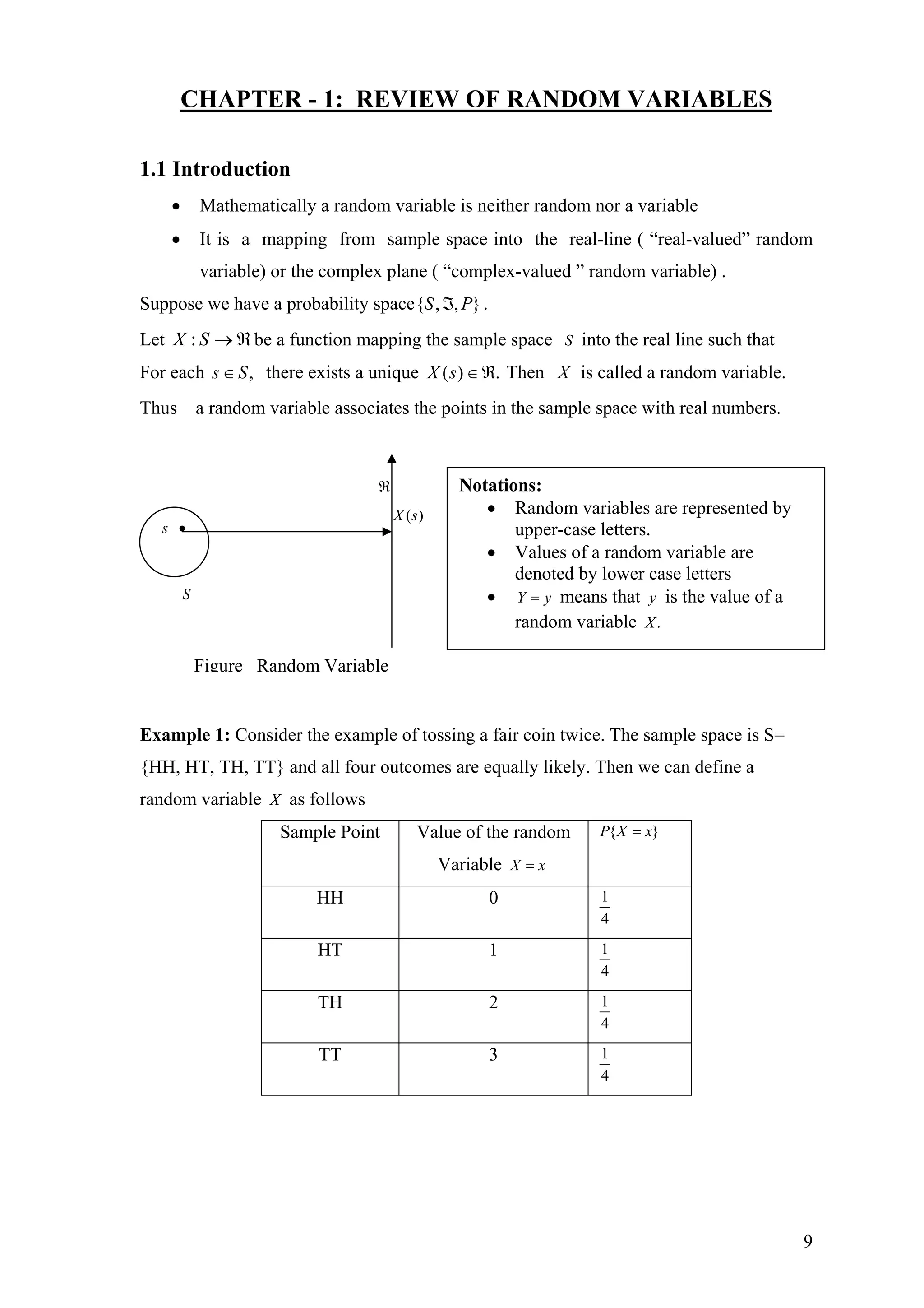
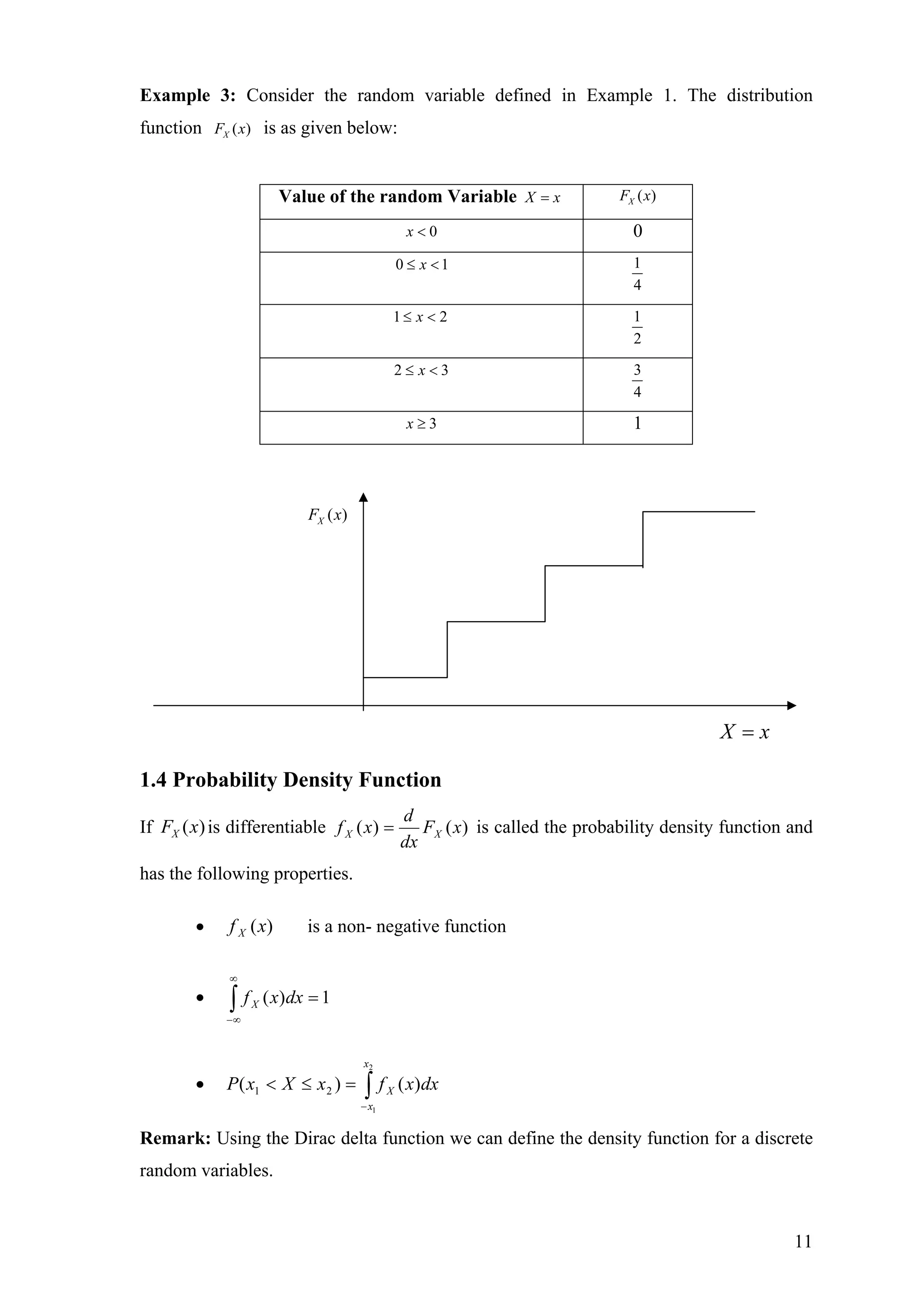
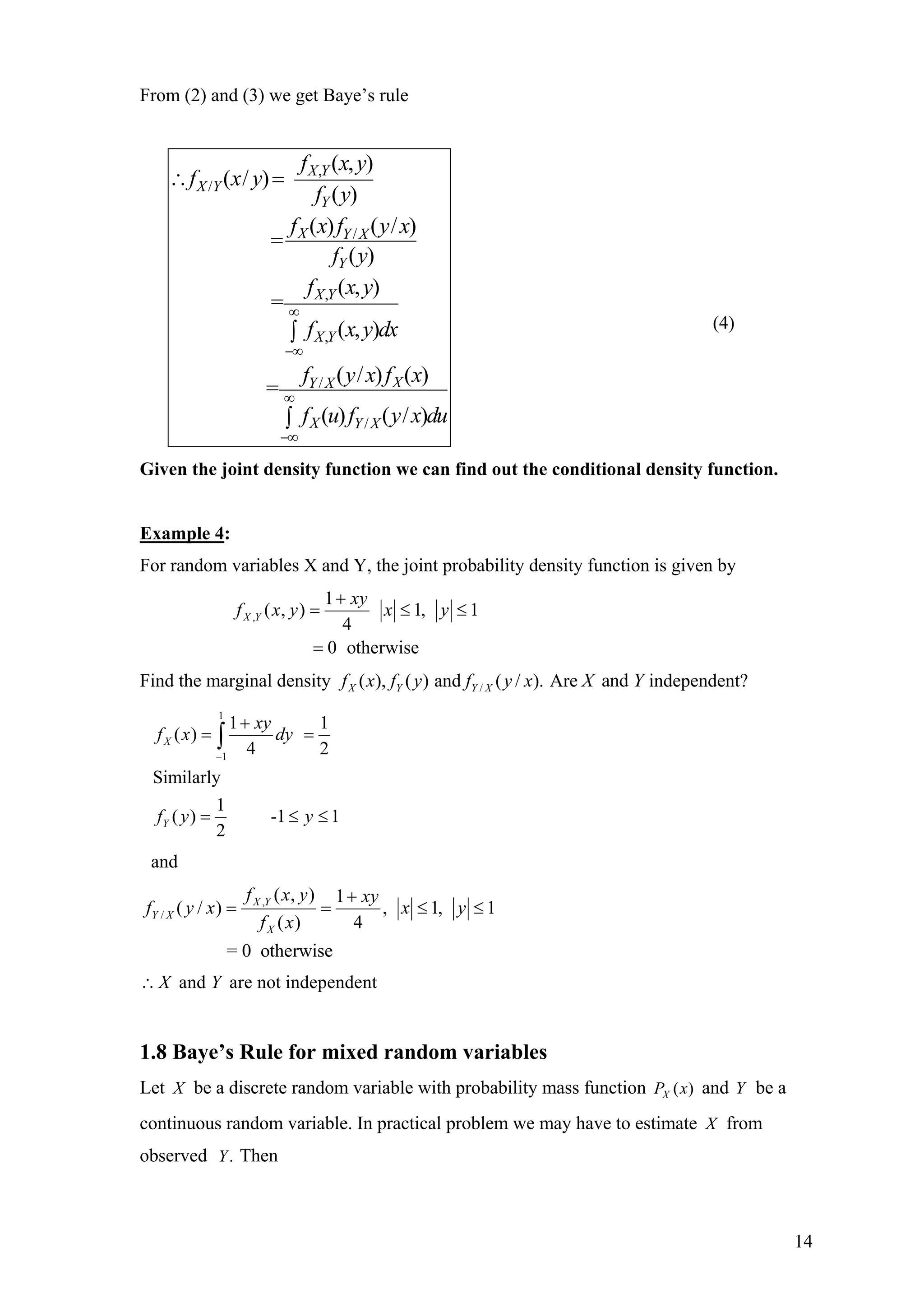
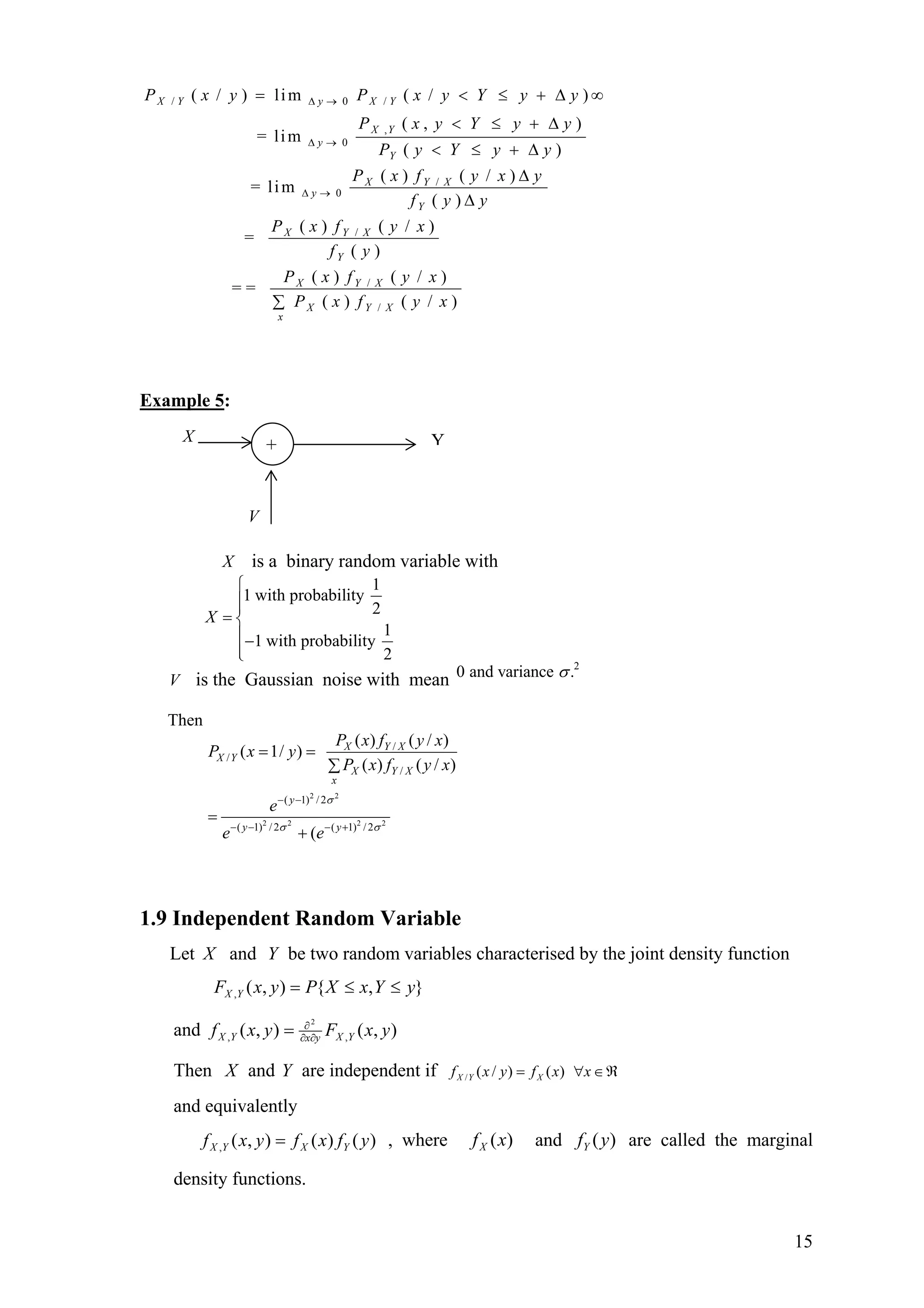
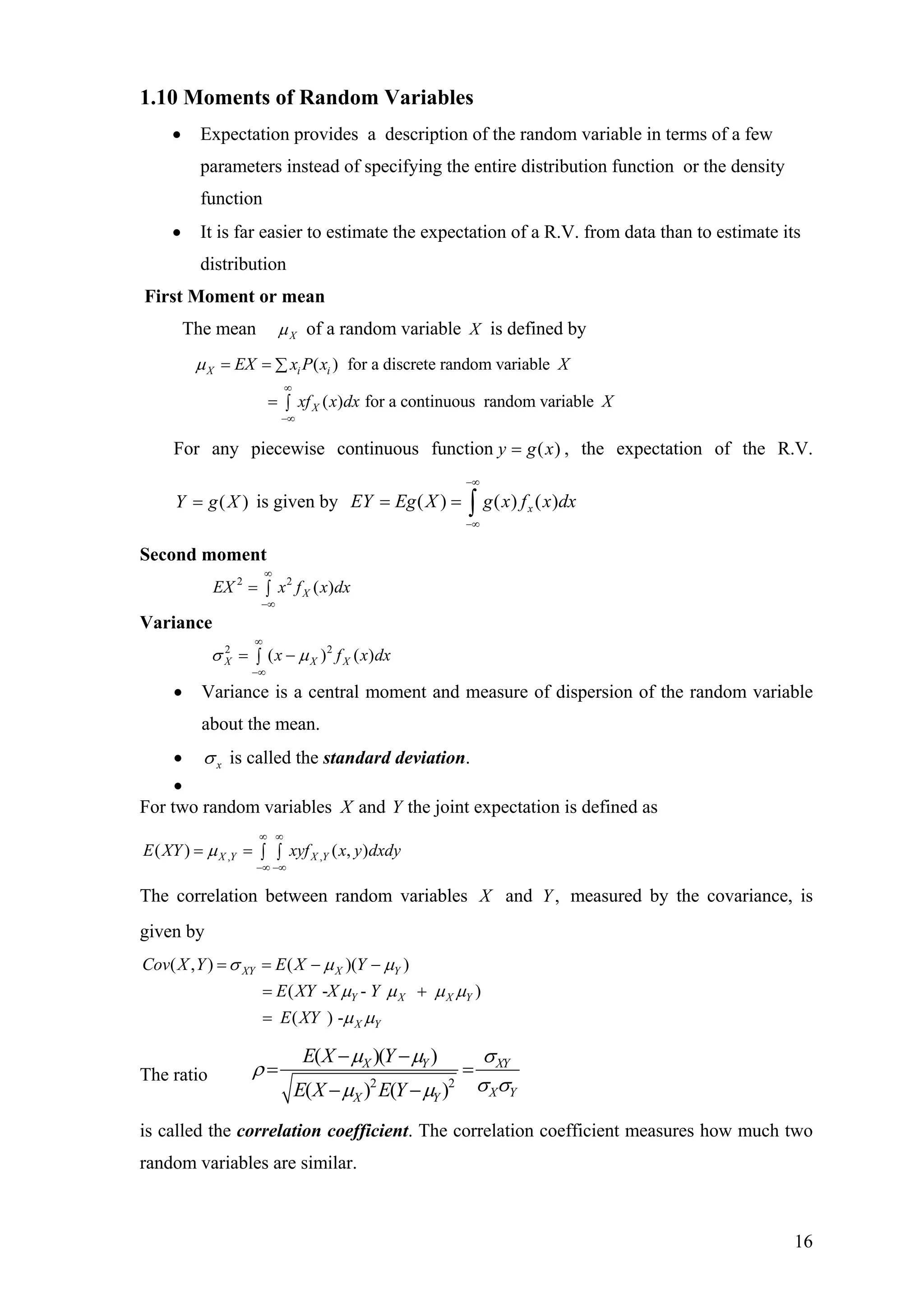
![1.28 Jointly Gaussian Random variables
Two random variables are called jointly Gaussian if their joint density function
is
YX and
2 2( ) ( )( ) ( )
1
2 2 22(1 ),
2
, ( , )
x x y y
X X Y Y
XY
X YX Y X Y
X Yf x y Ae
µ µ µ µ
σ σρ σ σ
ρ
− − − −
−
⎡ ⎤
− − +⎢ ⎥
⎢ ⎥⎣ ⎦
=
where 2
,12
1
YXyx
A
ρσπσ −
=
Properties:
(1) If X and Y are jointly Gaussian, then for any constants a and then the random
variable
,b
given by is Gaussian with mean,Z bYaXZ += YXZ ba µµµ += and variance
YXYXYXZ abba ,
22222
2 ρσσσσσ ++=
(2) If two jointly Gaussian RVs are uncorrelated, 0, =YXρ then they are statistically
independent.
)()(),(, yfxfyxf YXYX = in this case.
(3) If is a jointly Gaussian distribution, then the marginal densities),(, yxf YX
are also Gaussian.)(and)( yfxf YX
(4) If X and are joint by Gaussian random variables then the optimum nonlinear
estimator
Y
Xˆ of X that minimizes the mean square error is a linear
estimator
}]ˆ{[ 2
XXE −=ξ
aYX =ˆ
25](https://image.slidesharecdn.com/statisticalsignalprocessing1-151213044748/75/Statistical-signal-processing-1-25-2048.jpg)
![CHAPTER - 2 : REVIEW OF RANDOM PROCESS
2.1 Introduction
Recall that a random variable maps each sample point in the sample space to a point in
the real line. A random process maps each sample point to a waveform.
• A random process can be defined as an indexed family of random variables
{ ( ), }X t t T∈ whereT is an index set which may be discrete or continuous usually
denoting time.
• The random process is defined on a common probability space }.,,{ PS ℑ
• A random process is a function of the sample point ξ and index variable t and
may be written as ).,( ξtX
• For a fixed )),( 0tt = ,( 0 ξtX is a random variable.
• For a fixed ),( 0ξξ = ),( 0ξtX is a single realization of the random process and
is a deterministic function.
• When both andt ξ are varying we have the random process ).,( ξtX
The random process ),( ξtX is normally denoted by ).(tX
We can define a discrete random process [ ]X n on discrete points of time. Such a random
process is more important in practical implementations.
2( , )X t s3s
2s 1s
3( , )X t s
S
1( , )X t s
t
Figure Random Process
26](https://image.slidesharecdn.com/statisticalsignalprocessing1-151213044748/75/Statistical-signal-processing-1-26-2048.jpg)
![2.2 How to describe a random process?
To describe we have to use joint density function of the random variables at
different .
)(tX
t
For any positive integer , represents jointly distributed
random variables. Thus a random process can be described by the joint distribution
function
n )(),.....(),( 21 ntXtXtX n
and),.....,,.....,().....,( 212121)().....(),( 21
TtNntttxxxFxxxF nnnntXtXtX n
∈∀∈∀=
Otherwise we can determine all the possible moments of the process.
)())(( ttXE xµ= = mean of the random process at .t
))()((),( 2121 tXtXEttRX = = autocorrelation function at 21,tt
))(),(),((),,( 321321 tXtXtXEtttRX = = Triple correlation function at etc.,,, 321 ttt
We can also define the auto-covariance function of given by),( 21 ttCX )(tX
)()(),(
))()())(()((),(
2121
221121
ttttR
ttXttXEttC
XXX
XXX
µµ
µµ
−=
−−=
Example 1:
(a) Gaussian Random Process
For any positive integer represent jointly random
variables. These random variables define a random vector
The process is called Gaussian if the random vector
,n )(),.....(),( 21 ntXtXtX n
n
1 2[ ( ), ( ),..... ( )]'.nX t X t X t=X )(tX
1 2[ ( ), ( ),..... ( )]'nX t X t X t is jointly Gaussian with the joint density function given by
( )
' 1
1 2
1
2
( ), ( )... ( ) 1 2( , ,... )
2 det(
X
nX t X t X t n n
e
f x x x
π
−
−
=
XC X
XC )
Ewhere '( )( )= − −X X XC X µ X µ
and [ ]1 2( ) ( ), ( )...... ( ) '.nE E X E X E X= =Xµ X
(b) Bernouli Random Process
(c) A sinusoid with a random phase.
27](https://image.slidesharecdn.com/statisticalsignalprocessing1-151213044748/75/Statistical-signal-processing-1-27-2048.jpg)
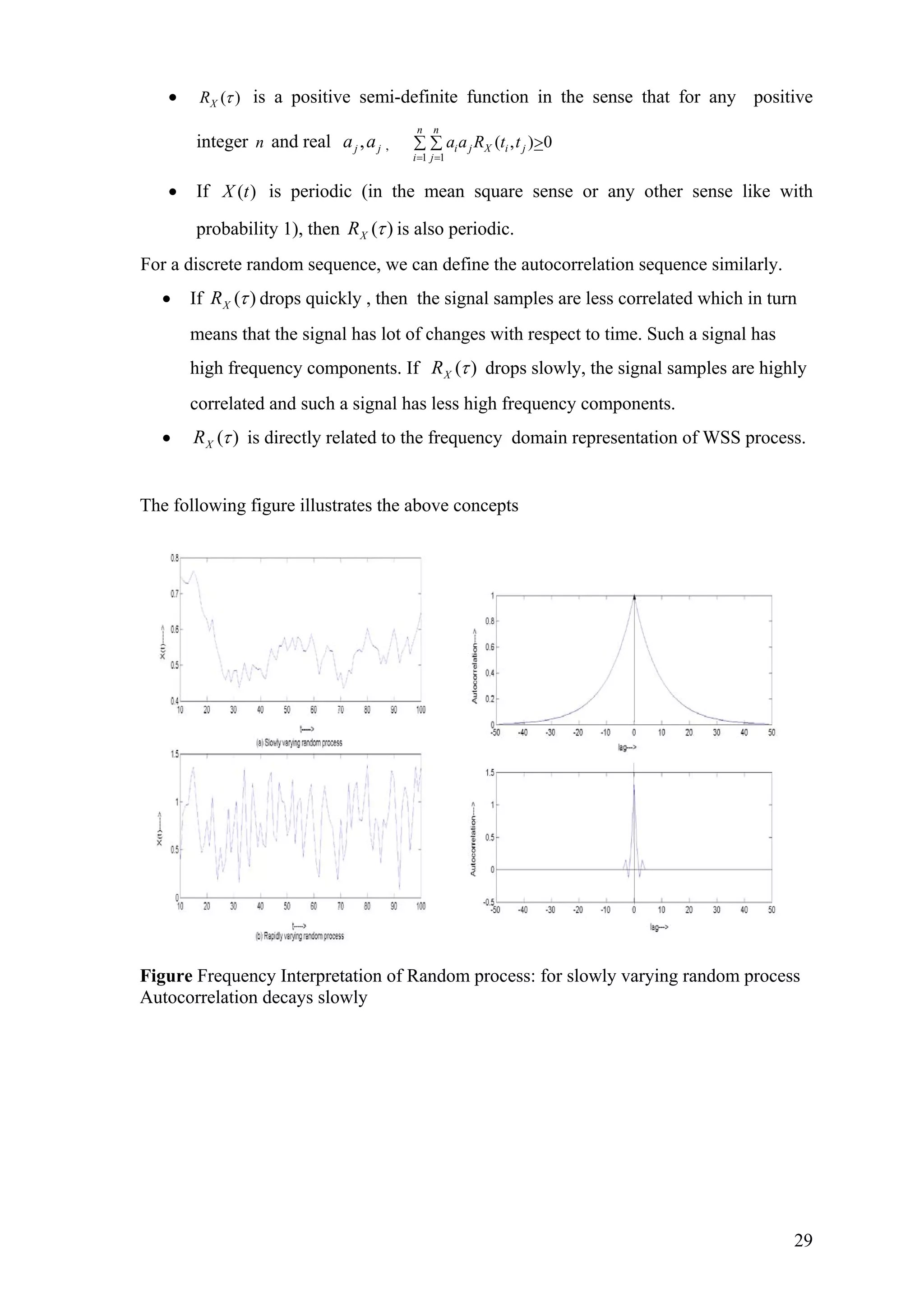
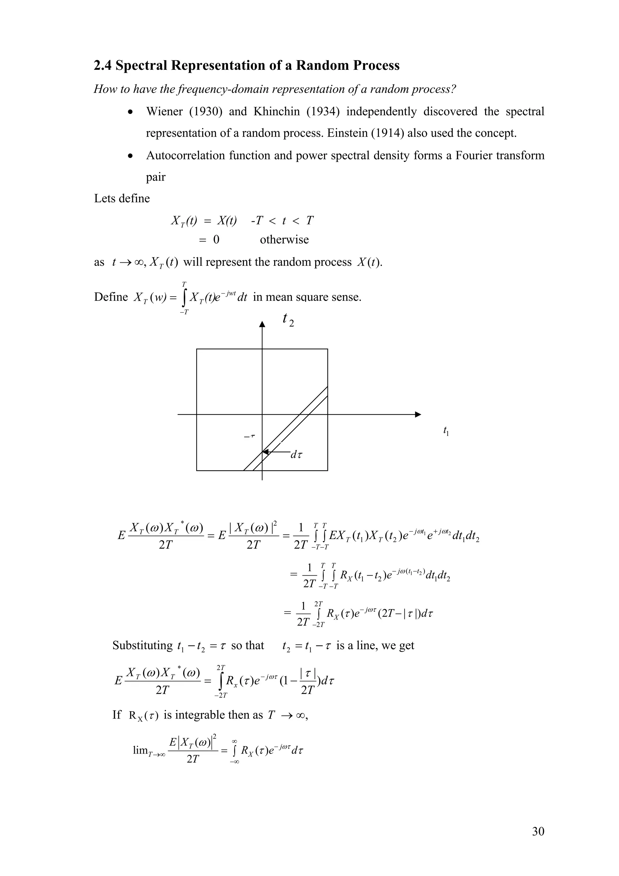
![*
, ,( ) ( )X Y Y XS w S w=
The Wiener-Khinchin theorem is also valid for discrete-time random processes.
If we define ][][][ nXmnE XmRX +=
Then corresponding PSD is given by
[ ]
[ ] 2
( )
or ( ) 1 1
j m
X x
m
j m
X x
m
S w R m e w
S f R m e f
ω
π
π π
∞
−
=−∞
∞
−
=−∞
= −∑
= −∑
≤ ≤
≤ ≤
1
[ ] ( )
2
j m
X XR m S w e
π
ω
ππ −
dw∫∴ =
For a discrete sequence the generalized PSD is defined in the domainz − as follows
[ ]( ) m
X x
m
S z R m z
∞
−
=−∞
= ∑
If we sample a stationary random process uniformly we get a stationary random sequence.
Sampling theorem is valid in terms of PSD.
Examples 2:
2 2
2
2
(1) ( ) 0
2
( ) -
(2) ( ) 0
1
( ) -
1 2 cos
a
X
X
m
X
X
R e a
a
S w w
a w
R m a a
a
S w w
a w a
τ
τ
π π
−
= >
= ∞ < <
+
= >
−
= ≤
− +
∞
≤
)
2.6 White noise process
S (x f
→ f
A white noise process is defined by)(tX
( )
2
X
N
S f f= −∞ < < ∞
The corresponding autocorrelation function is given by
( ) ( )
2
X
N
R τ δ τ= where )(τδ is the Dirac delta.
The average power of white noise
2
avg
N
P df
∞
−∞
= →∫ ∞
32](https://image.slidesharecdn.com/statisticalsignalprocessing1-151213044748/75/Statistical-signal-processing-1-32-2048.jpg)
![• Samples of a white noise process are uncorrelated.
• White noise is an mathematical abstraction, it cannot be realized since it has infinite
power
• If the system band-width(BW) is sufficiently narrower than the noise BW and noise
PSD is flat , we can model it as a white noise process. Thermal and shot noise are well
modelled as white Gaussian noise, since they have very flat psd over very wide band
(GHzs
• For a zero-mean white noise process, the correlation of the process at any lag 0≠τ is
zero.
• White noise plays a key role in random signal modelling.
• Similar role as that of the impulse function in the modeling of deterministic signals.
2.7 White Noise Sequence
For a white noise sequence ],[nx
( )
2
X
N
S w wπ π= − ≤ ≤
Therefore
( ) ( )
2
X
N
R m δ= m
where )(mδ is the unit impulse sequence.
White Noise WSS Random Signal
Linear
System
2.8 Linear Shi I va ia t yste ith Random Inputsft n r n S m w
Consider a discrete-time linear system with impulse response ].[nh
][][][
][][][
n* hnE xnE y
n* hnxny
=
=
For stationary input ][nx
0
[ ] [ ] [ ]
l
Y X X
k
E y n * h n h nµ µ µ
=
= = = ∑
2
N
2
N
2
N
( )XS ω
][nh
][nx
][ny
2
N
• • m• • →•
[ ]XR m
2
N
π ω→π−
33](https://image.slidesharecdn.com/statisticalsignalprocessing1-151213044748/75/Statistical-signal-processing-1-33-2048.jpg)
![where is the length of the impulse response sequencel
][*][*][
])[*][(*])[][(
][][][
mhmhmR
mnhmnxn* hnxE
mnynE ymR
X
Y
−=
−−=
−=
is a function of lag only.][mRY m
From above we get
w)SwΗ(wS XY (|(|= 2
))
)(wSXX
Example 3:
Suppose
X
( ) 1
0 otherwise
S ( )
2
c cH w w w
N
w w
= − ≤ ≤
=
= − ∞ ≤ ≤
w
∞
Then YS ( )
2
c c
N
w w w w= − ≤ ≤
and Y cR ( ) sinc(w )
2
N
τ τ=
2
)H(w
)(wSYY
)(τXR
τ
• Note that though the input is an uncorrelated process, the output is a correlated
process.
Consider the case of the discrete-time system with a random sequence as an input.][nx
][*][*][][ mhmhmRmR XY −=
Taking the we gettransform,−z
S )()()()( 1−
= zHzHzSz XY
Notice that if is causal, then is anti causal.)(zH )( 1−
zH
Similarly if is minimum-phase then is maximum-phase.)(zH )( 1−
zH
][nh
][nx ][ny
)(zH )( 1−
zH
][mRXX
][mRYY
][zSYY( )XXS z
34](https://image.slidesharecdn.com/statisticalsignalprocessing1-151213044748/75/Statistical-signal-processing-1-34-2048.jpg)
![Example 4:
If 1
1
( )
1
H z
zα −
=
−
and is a unity-variance white-noise sequence, then][nx
1
1
( ) ( ) ( )
1 1
1 21
YYS z H z H z
zz
1
α πα
−
−
=
⎛ ⎞⎛ ⎞
= ⎜ ⎟⎜ ⎟
−−⎝ ⎠⎝ ⎠
By partial fraction expansion and inverse −z transform, we get
||
2
1
1
][ m
Y amR
α−
=
2.9 Spectral factorization theorem
A stationary random signal that satisfies the Paley Wiener condition
can be considered as an output of a linea filter fed by a white noise
sequence.
][nX
| ln ( ) |XS w dw
π
π−
< ∞∫ r
If is an analytic function of ,)(wSX w
and , then| ln ( ) |XS w dw
π
π−
< ∞∫
2
( ) ( ) ( )X v c aS z H z H zσ=
where
)(zHc is the causal minimum phase transfer function
)(zHa is the anti-causal maximum phase transfer function
and 2
vσ a constant and interpreted as the variance of a white-noise sequence.
Innovation sequence
v n[ ] ][nX
Figure Innovation Filter
Minimum phase filter => the corresponding inverse filter exists.
)(zHc
Since is analytic in an annular region)(ln zSXX
1
zρ
ρ
< < ,
ln ( ) [ ] k
XX
k
S z c k z
∞
−
=−∞
= ∑
)
1
zHc
[ ]v n
(][nX
Figure whitening filter
35](https://image.slidesharecdn.com/statisticalsignalprocessing1-151213044748/75/Statistical-signal-processing-1-35-2048.jpg)
![where
1
[ ] ln ( )
2
iwn
XXc k S w e dwπ
π
π −= ∫ is the order cepstral coefficient.kth
For a real signal [ ] [ ]c k c k= −
and
1
[0] ln ( )
2
XXc Sπ
π
π −= ∫ w dw
1
1
1
[ ]
[ ] [ ]
[0]
[ ]
-1 2
( )
Let ( )
1 (1)z (2) ......
k
k
k k
k k
k
k
c k z
XX
c k z c k z
c
c k z
C
c c
S z e
e e e
H z e z
h h z
ρ
∞
−
=−∞
∞ −
− −
= =−∞
∞
−
=
∑
∑ ∑
∑
−
=
=
= >
= + + +
( [0] ( ) 1c z Ch Lim H z→∞= =∵
( )CH z and are both analyticln ( )CH z
=> is a minimum phase filter.( )CH z
Similarly let
1
1
( )
( )
1
( )
1
( )
k
k
a
k
k
c k z
c k z
C
H z e
e H z z
ρ
−
−
=−∞
∞
=
∑
∑
−
=
= = <
0)
2 1
Therefore,
( ) ( ) ( )XX V C CS z H z H zσ −
=
where 2 (c
V eσ =
Salient points
• can be factorized into a minimum-phase and a maximum-phase factors
i.e. and
)(zSXX
( )CH z 1
( )CH z−
.
• In general spectral factorization is difficult, however for a signal with rational
power spectrum, spectral factorization can be easily done.
• Since is a minimum phase filter, 1
( )CH z
exists (=> stable), therefore we can have a
filter
1
( )CH z
to filter the given signal to get the innovation sequence.
• and are related through an invertible transform; so they contain the
same information.
][nX [ ]v n
36](https://image.slidesharecdn.com/statisticalsignalprocessing1-151213044748/75/Statistical-signal-processing-1-36-2048.jpg)
![2.10 Wold’s Decomposition
Any WSS signal can be decomposed as a sum of two mutually orthogonal
processes
][nX
• a regular process [ ]rX n and a predictable process [ ]pX n , [ ] [ ] [ ]r pX n X n X n= +
• [ ]rX n can be expressed as the output of linear filter using a white noise
sequence as input.
• [ ]pX n is a predictable process, that is, the process can be predicted from its own
past with zero prediction error.
37](https://image.slidesharecdn.com/statisticalsignalprocessing1-151213044748/75/Statistical-signal-processing-1-37-2048.jpg)
![CHAPTER - 3: RANDOM SIGNAL MODELLING
3.1 Introduction
The spectral factorization theorem enables us to model a regular random process as
an output of a linear filter with white noise as input. Different models are developed
using different forms of linear filters.
• These models are mathematically described by linear constant coefficient
difference equations.
• In statistics, random-process modeling using difference equations is known as
time series analysis.
3.2 White Noise Sequence
The simplest model is the white noise . We shall assume that is of 0-
mean and variance
[ ]v n [ ]v n
2
.Vσ
[ ]VR m
3.3 Moving Average model model)(qMA
[ ]v n ][ nX
The difference equation model is
[ ] [ ]
q
i
i o
X n b v n
=
i= −∑
2 2 2
0
0 0
and [ ] is an uncorrelated sequence means
e X
q
X i V
i
v n
b
µ µ
σ σ
=
= ⇒ =
= ∑
The autocorrelations are given by
• • • • m
FIR
filter
( )VS w 2
w
2
Vσ
π
38](https://image.slidesharecdn.com/statisticalsignalprocessing1-151213044748/75/Statistical-signal-processing-1-38-2048.jpg)
![0 0
0 0
[ ] [ ] [ ]
[ ] [ ]
[ ]
X
q q
i j
i j
q q
i j V
i j
R m E X n X n - m
bb Ev n i v n m j
bb R m i j
= =
= =
=
= − − −∑ ∑
= − +∑ ∑
Noting that 2
[ ] [ ]V VR m σ δ= m , we get
2
[ ] when
0
V VR m
m-i j
i m j
σ=
+ =
⇒ = +
The maximum value for so thatqjm is+
2
0
[ ] 0
and
[ ] [ ]
q m
X j j m V
j
X X
R m b b m
R m R m
σ
−
+
=
= ≤∑
− =
q≤
Writing the above two relations together
2
0
[ ]
= 0 otherwise
q m
X j vj m
j
R m b b mσ
−
+
=
q= ≤∑
Notice that, [ ]XR m is related by a nonlinear relationship with model parameters. Thus
finding the model parameters is not simple.
The power spectral density is given by
2
2
( ) ( )
2
V
XS w B w
σ
π
= , where jqw
q
jw
ebebbwB −−
1 ++== ......)( ο
FIR system will give some zeros. So if the spectrum has some valleys then MA will fit
well.
3.3.1 Test for MA process
[ ]XR m becomes zero suddenly after some value of .m
[ ]XR m
m
Figure: Autocorrelation function of a MA process
39](https://image.slidesharecdn.com/statisticalsignalprocessing1-151213044748/75/Statistical-signal-processing-1-39-2048.jpg)
![Figure: Power spectrum of a MA process
Example 1: MA(1) process
1 0
0 1
2 2 2
1 0
1 0
[ ] [ 1] [ ]
Here the parameters b and are tobe determined.
We have
[1]
X
X
X n b v n b v n
b
b b
R b b
σ
= − +
= +
=
From above can be calculated using the variance and autocorrelation at lag 1 of
the signal.
0 andb 1b
3.4 Autoregressive Model
In time series analysis it is called AR(p) model.
The model is given by the difference equation
1
[ ] [ ] [ ]
p
i
i
X n a X n i v
=
= − +∑ n
The transfer function is given by)(wA
q m→
[ ]XR m( )XS w
ω→
][nXIIR
filter
[ ]v n
40](https://image.slidesharecdn.com/statisticalsignalprocessing1-151213044748/75/Statistical-signal-processing-1-40-2048.jpg)
![1
1
( )
1
n
j i
i
i
A w
a e ω−
=
=
− ∑
with (all poles model) and10 =a
2
2
( )
2 | ( ) |
e
XS w
A
σ
π ω
=
If there are sharp peaks in the spectrum, the AR(p) model may be suitable.
The autocorrelation function [ ]XR m is given by
1
2
1
[ ] [ ] [ ]
[ ] [ ] [ ] [ ]
[ ] [ ]
X
p
i
i
p
i X V
i
R m E X n X n - m
a EX n i X n m Ev n X n m
a R m i mσ δ
=
=
=
= − − + −∑
= − +∑
2
1
[ ] [ ] [ ]
p
X i X V
i
R m a R m i mσ δ
=
∴ = − +∑ Im ∈∨
The above relation gives a set of linear equations which can be solved to find s.ia
These sets of equations are known as Yule-Walker Equation.
Example 2: AR(1) process
1
2
1
2
1
1
1
2
2
X 2
2
2
[ ] [ 1] [ ]
[ ] [ 1] [ ]
[0] [ 1] (1)
and [1] [0]
[1]
so that
[0]
From (1) [0]
1-
After some arithmatic we get
[ ]
1-
X X V
X X V
X X
X
X
V
X
m
V
X
X n a X n v n
R m a R m m
R a R
R a R
R
a
R
R
a
a
R m
a
σ δ
σ
σ
σ
σ
= − +
= − +
∴ = − +
=
=
= =
=
ω→
( )XS ω
[ ]XR m
m→
41](https://image.slidesharecdn.com/statisticalsignalprocessing1-151213044748/75/Statistical-signal-processing-1-41-2048.jpg)
![3.5 ARMA(p,q) – Autoregressive Moving Average Model
Under the most practical situation, the process may be considered as an output of a filter
that has both zeros and poles.
The model is given by
1 0
[ ] [ ] [ ]
p q
i i
i i
x n a X n i b v n
= =
= − +∑ ∑ i− (ARMA 1)
and is called the model.),( qpARMA
The transfer function of the filter is given by
2 2
2
( )
( )
( )
( )
( )
( ) 2
V
X
B
H w
A
B
S w
A
ω
ω
ω σ
ω π
=
=
How do get the model parameters?
For m there will be no contributions from terms to),1max( +≥ p, q ib [ ].XR m
1
[ ] [ ] max( , 1)
p
X i X
i
R m a R m i m p q
=
= − ≥ +∑
From a set of p Yule Walker equations, parameters can be found out.ia
Then we can rewrite the equation
∑ −=∴
∑ −+=
=
=
q
i
i
p
i
i
invbnX
inXanXnX
0
1
][][
~
][][][
~
From the above equation b can be found out.si
The is an economical model. Only only model may
require a large number of model parameters to represent the process adequately. This
concept in model building is known as the parsimony of parameters.
),( qpARMA )( pAR )(qMA
The difference equation of the model, given by eq. (ARMA 1) can be
reduced to
),( qpARMA
p first-order difference equation give a state space representation of the
random process as follows:
[ 1] [
[ ] [ ]
]Bu n
X n n
− +
=
z[n] = Az n
Cz
where
)(
)(
)(
wA
wB
wH =
[ ]X n
[ ]v n
42](https://image.slidesharecdn.com/statisticalsignalprocessing1-151213044748/75/Statistical-signal-processing-1-42-2048.jpg)
![1 2
0 1
[ ] [ [ ] [ 1].... [ ]]
......
0 1......0
, [1 0...0] and
...............
0 0......1
[ ... ]
p
q
x n X n X n p
a a a
b b b
′= − −
⎡ ⎤
⎢ ⎥
⎢ ⎥ ′= =
⎢ ⎥
⎢ ⎥
⎢ ⎥⎣ ⎦
=
z n
A B
C
Such representation is convenient for analysis.
3.6 General Model building Steps),( qpARMA
• Identification of p and q.
• Estimation of model parameters.
• Check the modeling error.
• If it is white noise then stop.
Else select new values for p and q
and repeat the process.
3.7 Other model: To model nonstatinary random processes
• ARIMA model: Here after differencing the data can be fed to an ARMA
model.
• SARMA model: Seasonal ARMA model etc. Here the signal contains a
seasonal fluctuation term. The signal after differencing by step equal to the
seasonal period becomes stationary and ARMA model can be fitted to the
resulting data.
43](https://image.slidesharecdn.com/statisticalsignalprocessing1-151213044748/75/Statistical-signal-processing-1-43-2048.jpg)
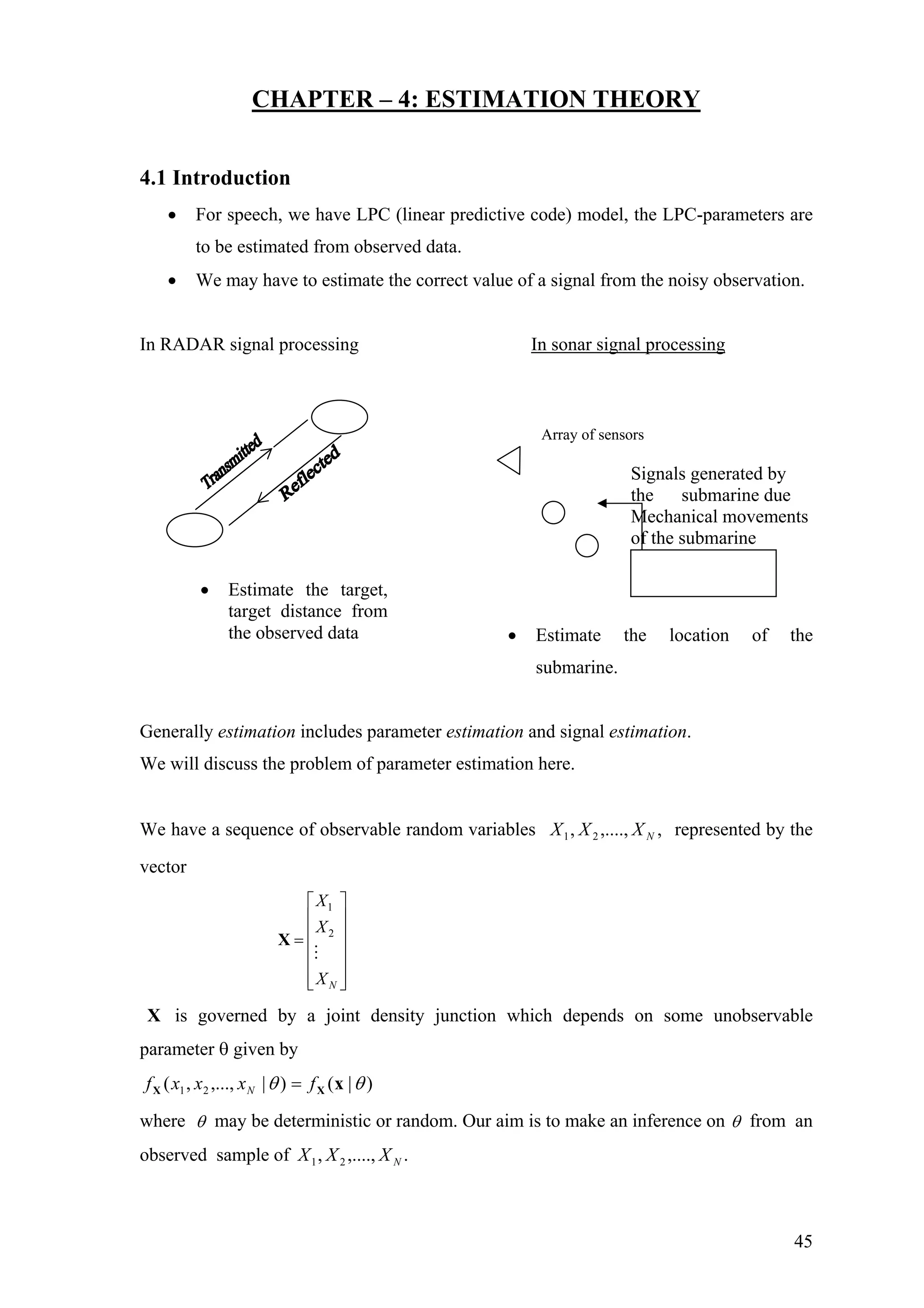
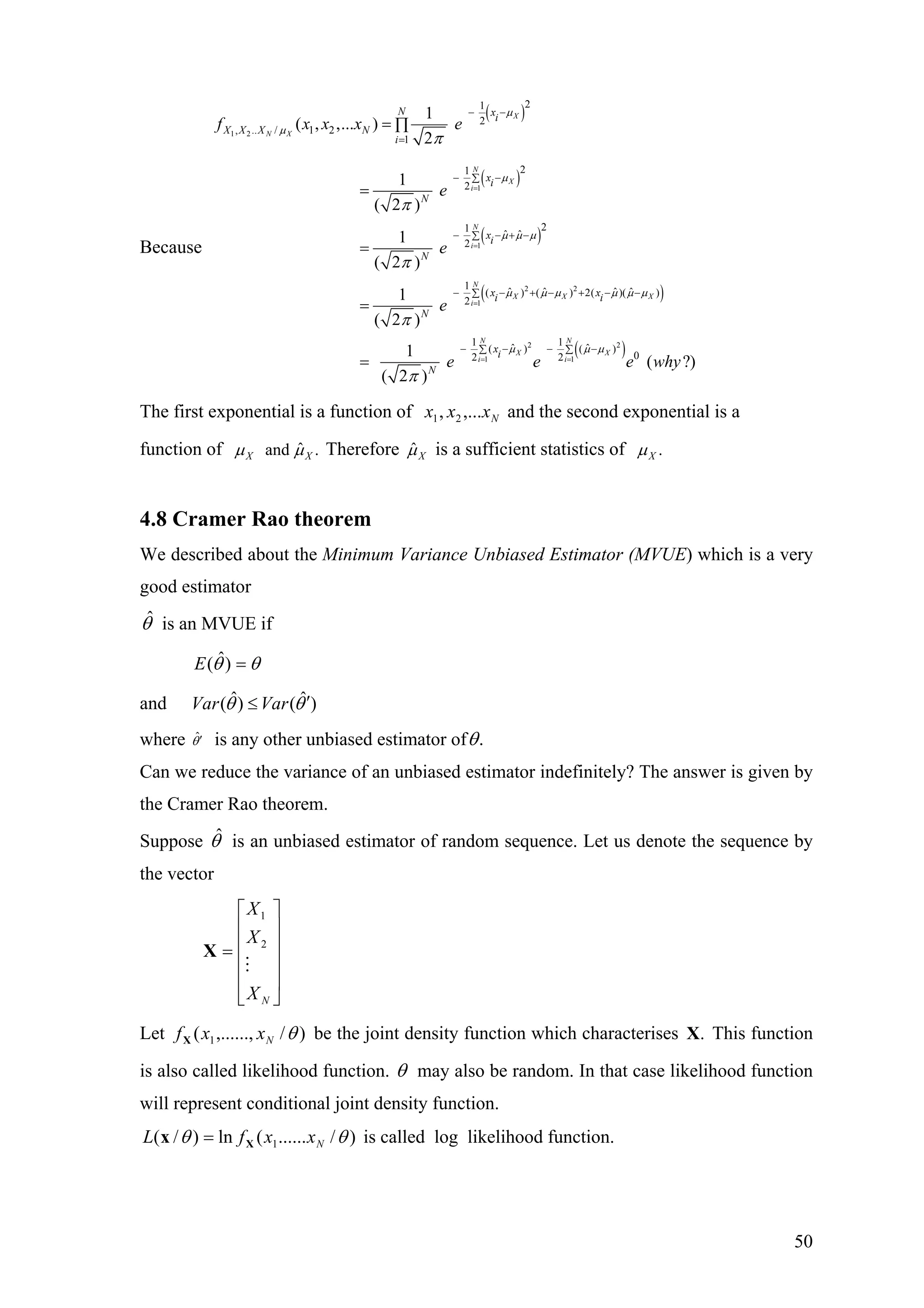
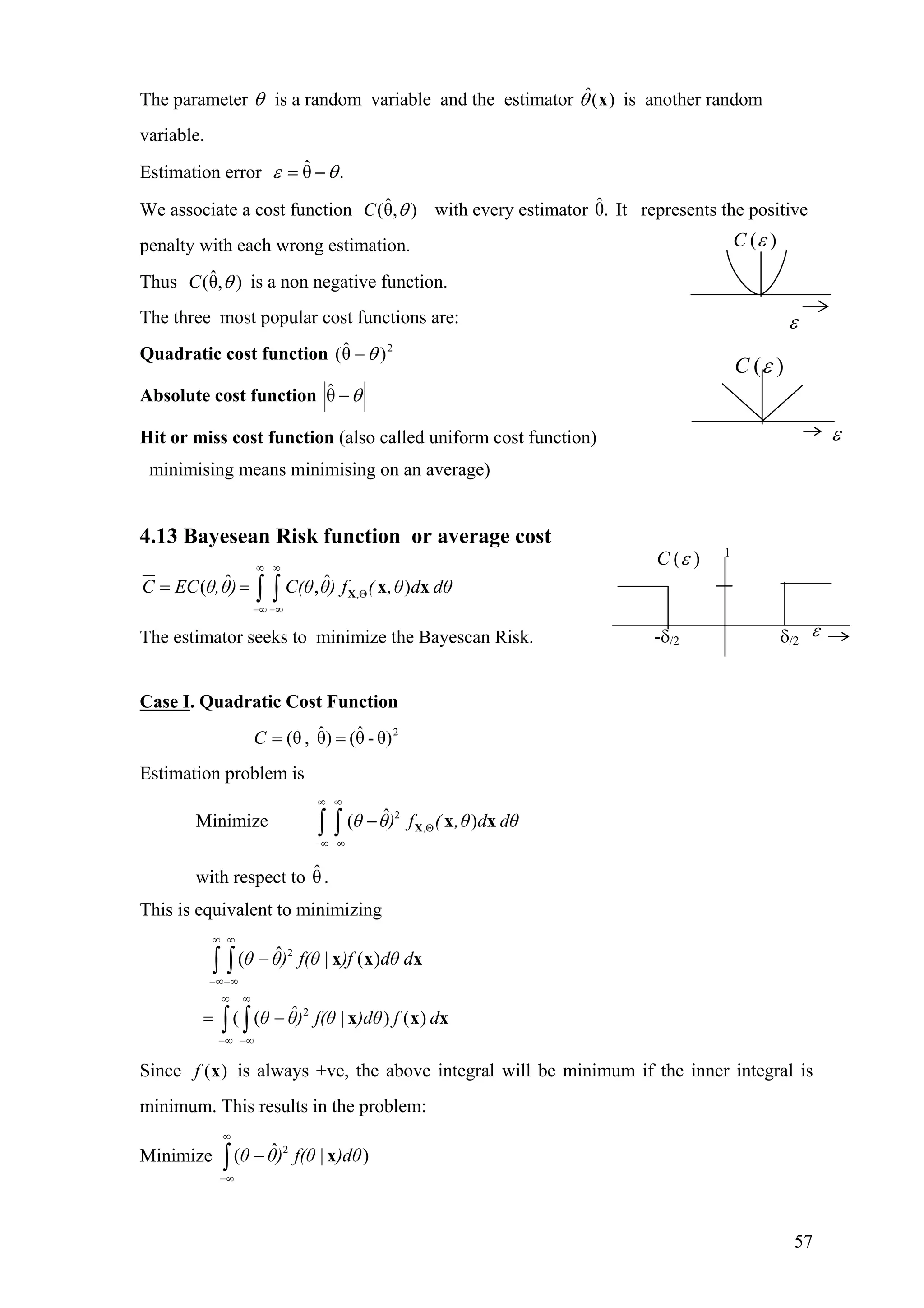
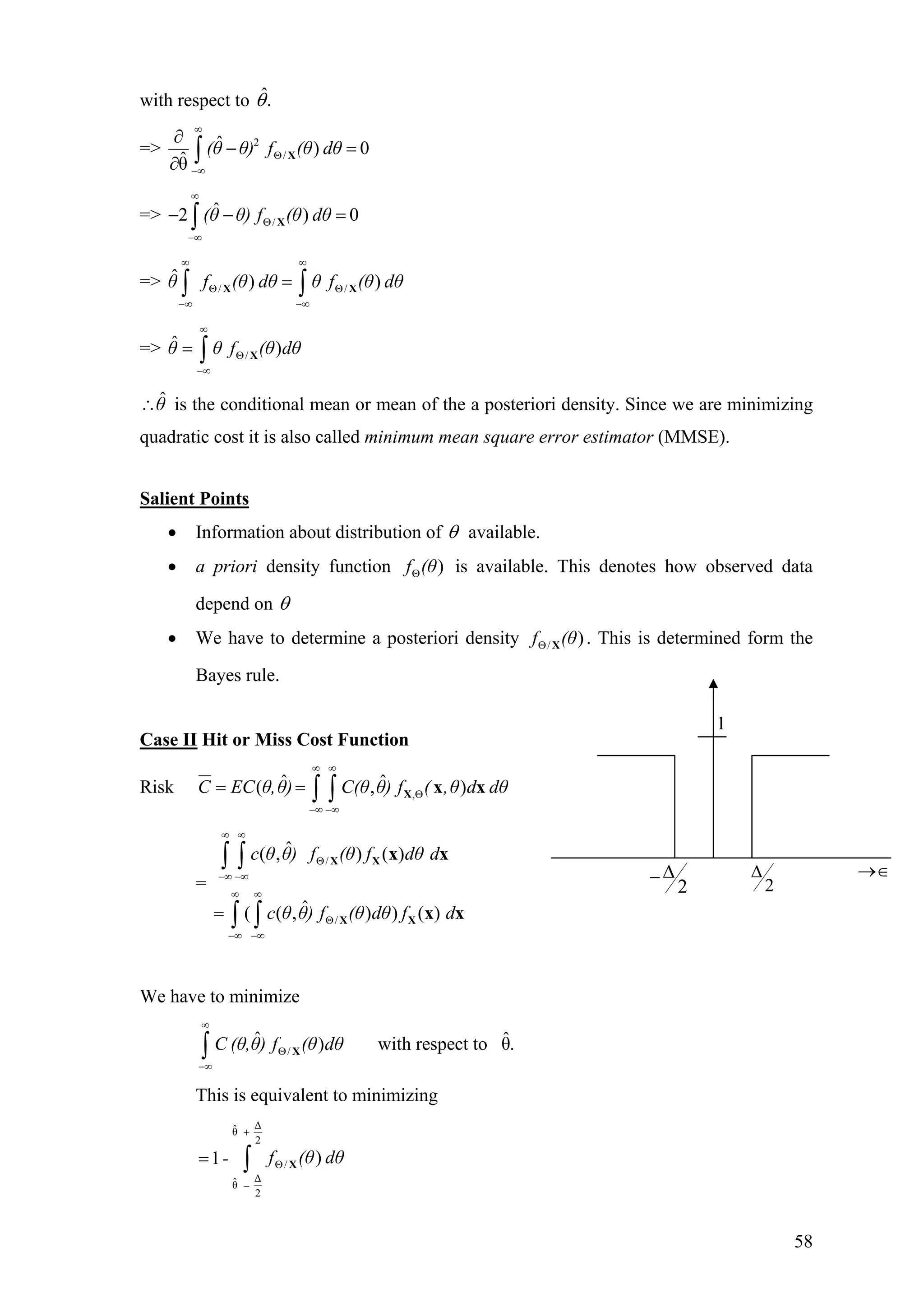
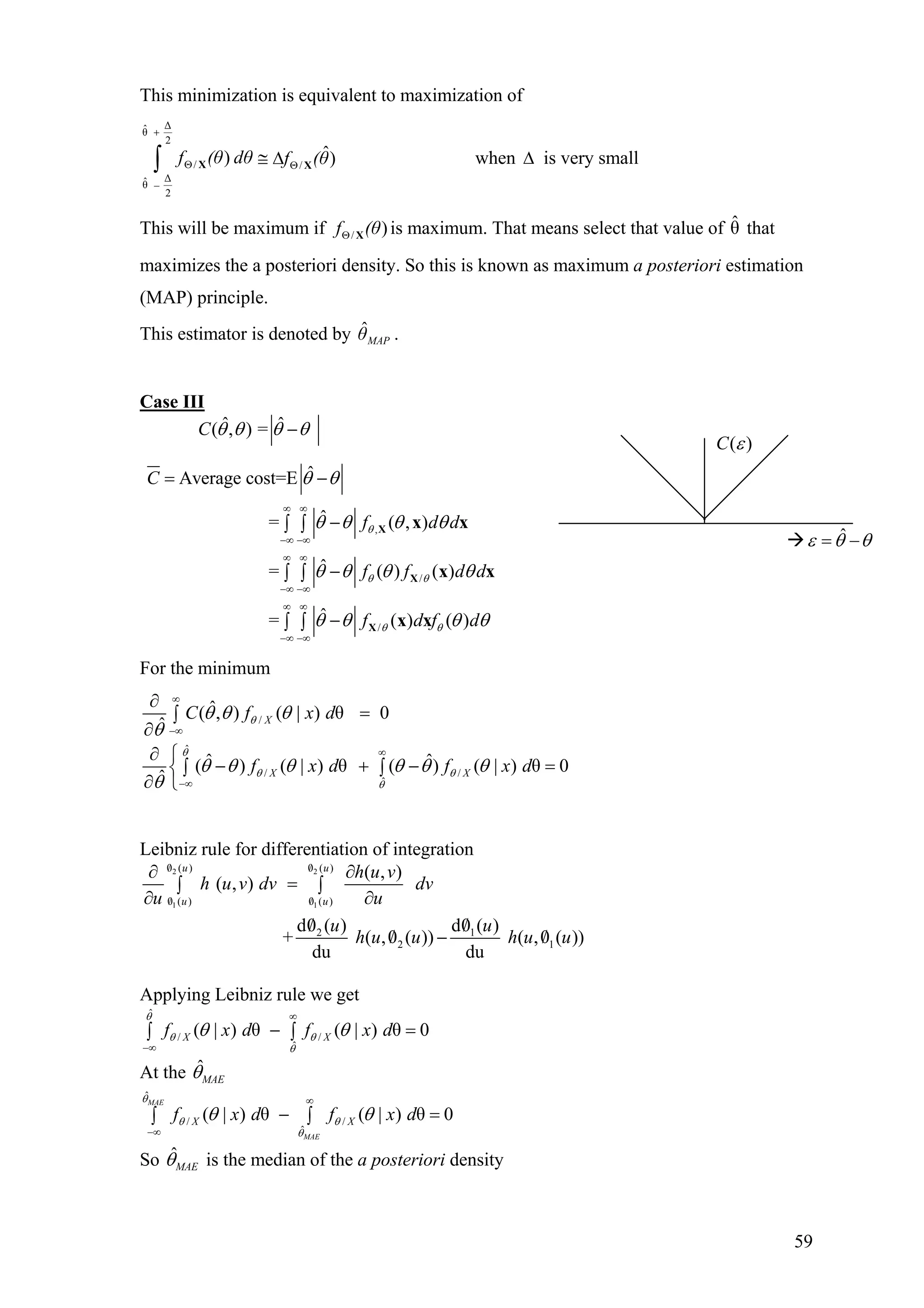
![] MAP
ˆ/ θ
MAP
ln (x) 0
θ
1ˆ
Xf
X
θ
λ
Θ
∂
=
∂
⇒ =
+
Example 8: Binary Communication problem
X is a binary random variable with
1 with probability 1/2
1 with probability 1/ 2
X
⎧
= ⎨
−⎩
V is the Gaussian noise with mean
2
0 and variance .σ
To find the MSE for X from the observed data .Y
Then
2 2
2 2
2 2 2 2
( ) / 2
/
/
/
/
( ) / 2
( 1) / 2 ( 1) / 2
1
( ) [ ( 1) ( 1)]
2
1
( / )
2
( ) ( / )
( / )
( ) ( / )
[ ( 1) ( 1)]
x
y x
Y X
X Y X
X Y
X Y X
y x
y y
f x x x
f y x e
f x f y x
f x y
f x f y x fx
e x x
e e
σ
σ
σ σ
δ δ
πσ
δ δ
− −
∞
−∞
− −
− − − +
= − + +
=
=
∫
− + +
=
+
Hence
2 2
2 2 2 2
2 2 2 2
2 2 2 2
( ) / 2
( 1) / 2 ( 1) / 2
( 1) / 2 ( 1) / 2
( 1) /2 ( 1) /2
2
[ ( 1) ( 1)]ˆ ( / )
=
tanh( / )
y x
MMSE y y
y y
y y
e x x
X E X Y x dx
e e
e e
e e
y
σ
σ σ
σ σ
σ σ
δ δ
σ
− −∞
− − − +
−∞
− − − +
− − − +
− + +
= = ∫
+
−
+
=
Y+X
V
61](https://image.slidesharecdn.com/statisticalsignalprocessing1-151213044748/75/Statistical-signal-processing-1-61-2048.jpg)
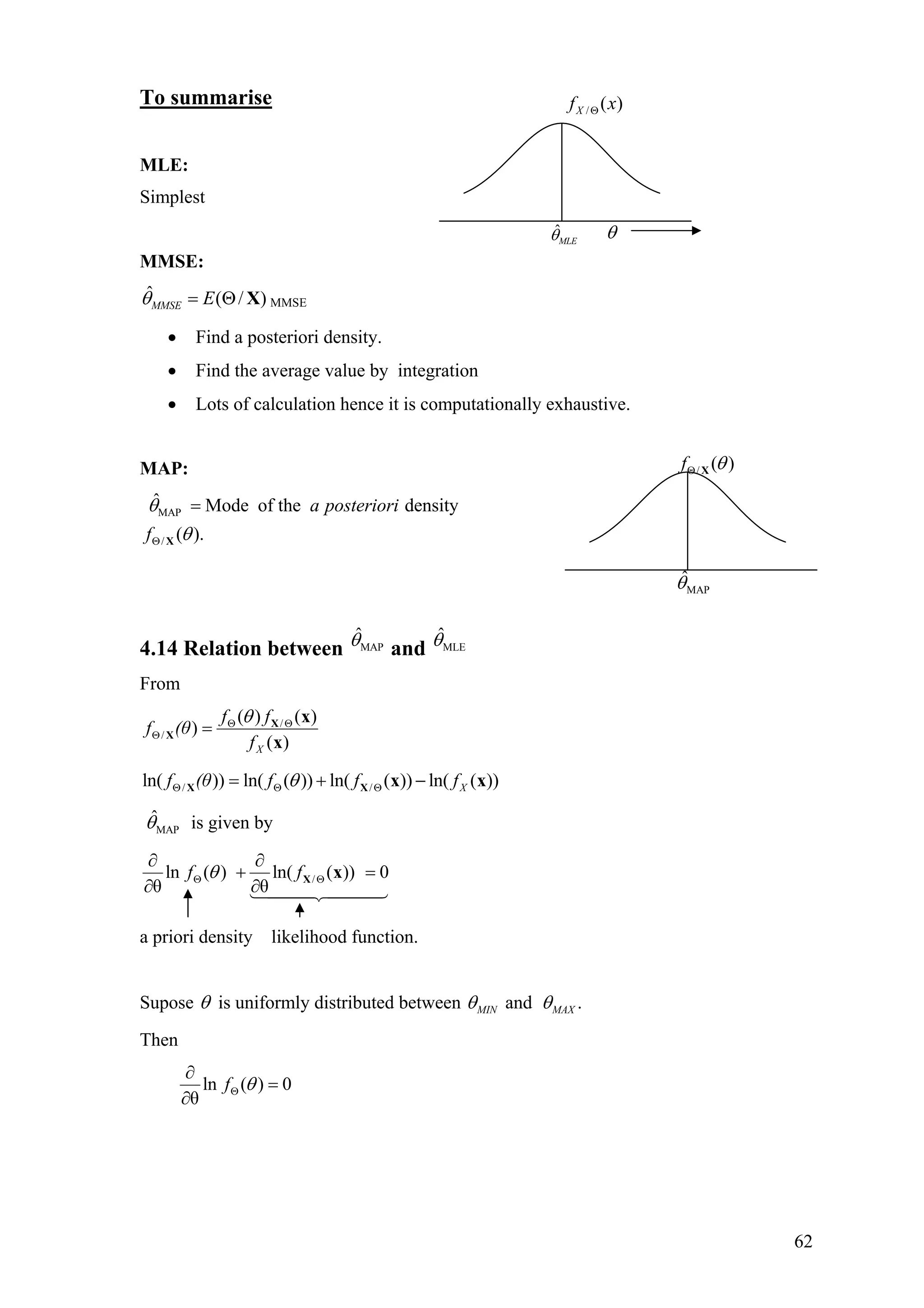
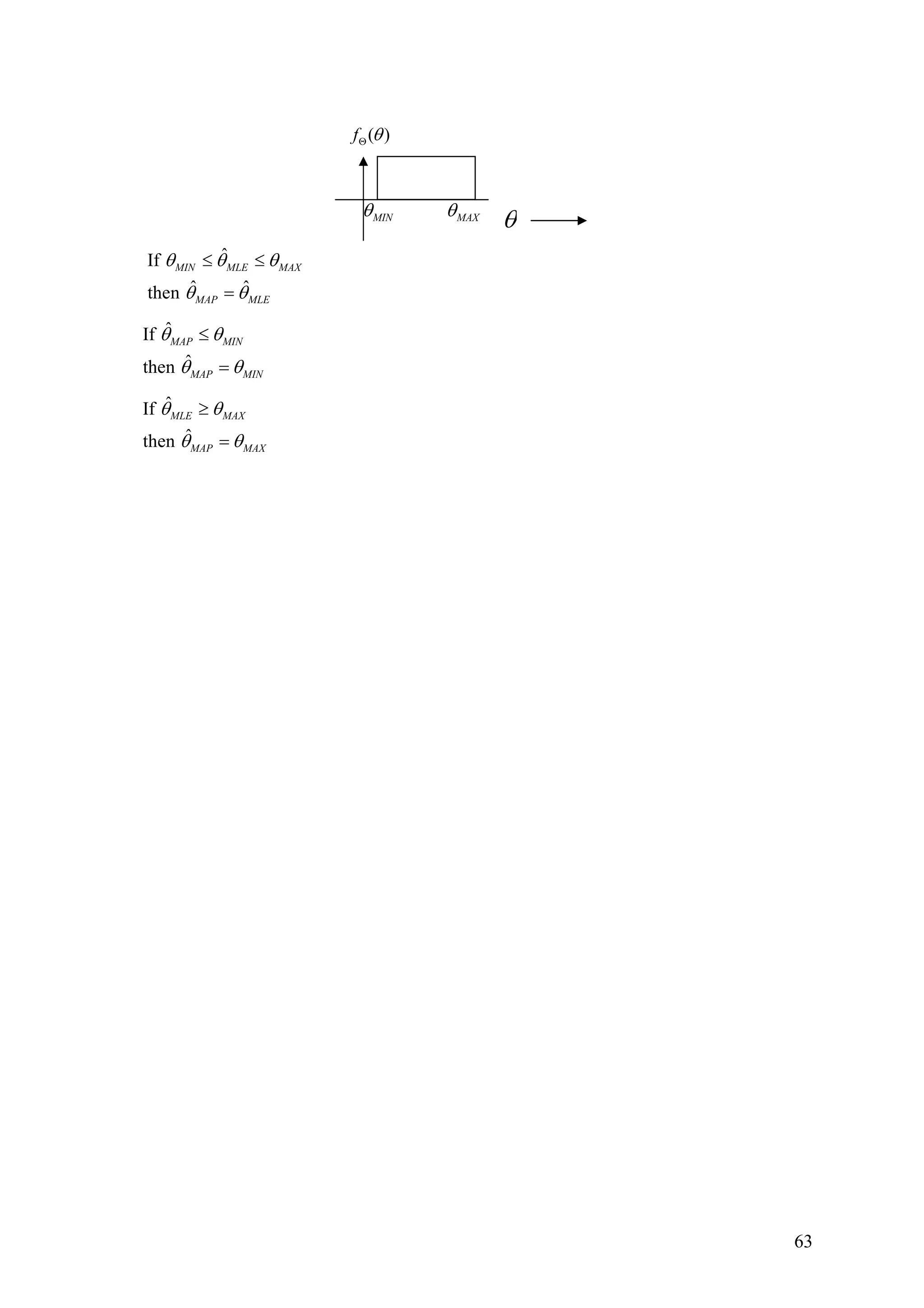

![CHAPTER – 5: WIENER FILTER
5.1 Estimation of signal in presence of white Gaussian noise (WGN)
Consider the signal model is
][][][ nVnXnY +=
where is the observed signal, is 0-mean Gaussian with variance 1 and][nY ][nX ][nV
is a white Gaussian sequence mean 0 and variance 1. The problem is to find the best
guess for given the observation][nX [ ], 1,2,...,Y i i n=
Maximum likelihood estimation for determines that value of for which the
sequence is most likely. Let us represent the random sequence
by the random vector
][nX ][nX
[ ], 1,2,...,Y i i n=
[ ], 1,2,...,Y i i n=
[ ] [ [ ], [ 1],.., [1]]'
and the value sequence [1], [2],..., [ ] by
[ ] [ [ ], [ 1],.., [1]]'.
Y n Y n Y
y y y n
y n y n y
= −
= −
Y n
y n
The likelihood function / [ ] ( [ ]/ [ ])n X nf n x nY[ ] y will be Gaussian with mean ][nx
( )
2
1
( [ ] [ ])
2
/ [ ]
1
( [ ]/ [ ])
2
n
i
y i x n
n X n n
f n x n e
π
=
−
−∑
=Y[ ] y
Maximum likelihood will be given by
[1], [2],..., [ ]/ [ ] ˆ [ ]
( ( [1], [2],..., [ ]) / [ ]) 0
[ ] MLE
Y Y Y n X n x n
f y y y n x n
x n
∂
=
∂
1
1
ˆ [ ] [ ]
n
MLE
i
n y
n
χ
=
⇒ = ∑ i
Similarly, to find ][ˆ nMAPχ and ˆ [ ]MMSE nχ we have to find a posteriori density
2
2
1
[ ] [ ]/ [ ]
[ ]/ [ ]
[ ]
1 ( [ ] [ ])
[ ]
2 2
[ ]
( [ ]) ( [ ]/ [ ])
( [ ]/ [ ])
( [ ])
1
=
( [ ])
n
i
X n n X n
X n n
n
y i x n
x n
n
f x n f n x n
f x n
f n
e
f n
=
−
− −
=
∑
Y
Y
Y
Y
y
y n
y
y
Taking logarithm
X Y
V
+
65](https://image.slidesharecdn.com/statisticalsignalprocessing1-151213044748/75/Statistical-signal-processing-1-65-2048.jpg)
![2
2
[ ]/ [ ] [ ]
1
1 ( [ ] [ ])
log ( [ ]) [ ] log ( [ ])
2 2
n
e X n n e n
i
y i x n
f x n x n f n
=
−
= − − −∑Y Y y
[ ]/ [ ]log ( [ ])e X n nf x nY is maximum at ˆ [ ].MAPx n Therefore, taking partial derivative of
[ ]/ [ ]log ( [ ])e X n nf x nY with respect to [ ]x n and equating it to 0, we get
1 ˆ [ ]
1
MAP
[ ] ( [ ] [ ]) 0
[ ]
ˆ [ ]
1
MAP
n
i x n
n
i
x n y i x n
y i
x n
n
=
=
− −
=
+
∑
∑
=
Similarly the minimum mean-square error estimator is given by
1
MMSE
[ ]
ˆ [ ] ( [ ]/ [ ])
1
n
i
y i
x n E X n n
n
=
= =
+
∑
y
• For MMSE we have to know the joint probability structure of the channel and the
source and hence the a posteriori pdf.
• Finding pdf is computationally very exhaustive and nonlinear.
• Normally we may be having the estimated values first-order and second-order
statistics of the data
We look for a simpler estimator.
The answer is Optimal filtering or Wiener filtering
We have seen that we can estimate an unknown signal (desired signal) [ ]x n from an
observed signal on the basis of the known joint distributions of and[ ]y n [ ]y n [ ].x n We
could have used the criteria like MMSE or MAP that we have applied for parameter es
timations. But such estimations are generally non-linear, require the computation of a
posteriori probabilities and involves computational complexities.
The approach taken by Wiener is to specify a form for the estimator that depends on a
number of parameters. The minimization of errors then results in determination of an
optimal set of estimator parameters. A mathematically sample and computationally easier
estimator is obtained by assuming a linear structure for the estimator.
66](https://image.slidesharecdn.com/statisticalsignalprocessing1-151213044748/75/Statistical-signal-processing-1-66-2048.jpg)
![5.2 Linear Minimum Mean Square Error Estimator
The linear minimum mean square error criterion is illustrated in the above figure. The
problem can be slated as follows:
Given observations of data determine a set of
parameters such that
[ 1], [ 2].. [ ],... [ ],y n M y n M y n y n N− + − + +
[ 1], [ 2]..., [ ],... [ ]h M h M h o h N− − −
1
ˆ[ ] [ ] [ ]
M
i N
x n h i y n
−
=−
= −∑ i
and the mean square error ( )
2
ˆ[ ] [ ]E x n x n− is a minimum with respect to
[ ], [ 1]...., [ ], [ ],..., [ 1].h N h N h o h i h M− − + −
This minimization problem results in an elegant solution if we assume joint stationarity of
the signals [ ] and [ ]x n y n . The estimator parameters can be obtained from the second
order statistics of the processes [ ] and [ ].x n y n
The problem of deterring the estimator parameters by the LMMSE criterion is also called
the Wiener filtering problem. Three subclasses of the problem are identified
Noise
Filter
[ ]x n [ ]y n ˆ[ ]x n
Syste
m
+
[ 1]y n M− − …….. …[ ]y n
1n M− − n n N+
1. The optimal smoothing problem 0N >
2. The optimal filtering problem 0N =
3. The optimal prediction problem 0N <
67](https://image.slidesharecdn.com/statisticalsignalprocessing1-151213044748/75/Statistical-signal-processing-1-67-2048.jpg)
![In the smoothing problem, an estimate of the signal inside the duration of observation of
the signal is made. The filtering problem estimates the curent value of the signal on the
basis of the present and past observations. The prediction problem addresses the issues of
optimal prediction of the future value of the signal on the basis of present and past
observations.
5.3 Wiener-Hopf Equations
The mean-square error of estimation is given by
2 2
1
2
ˆ[ ] ( [ ] [ ])
( [ ] [ ] [ ])
M
i N
Ee n E x n x n
E x n h i y n i
−
=−
= −
= − −∑
We have to minimize with respect to each to get the optimal estimation.][2
nEe ][ih
Corresponding minimization is given by
{ }2
[ ]
0, for ..0.. 1
[ ]
E e n
j N M
h j
∂
= = −
∂
−
( E being a linear operator, and
[ ]
E
h j
∂
∂
can be interchanged)
[ ] [ - ] 0, ...0,1,... 1Ee n y n j j N M= = − − (1)
or
[ ]
1
[ ] - [ ] [ ] [ - ] 0, ...0,1,... 1
a
e n
M
i N
E x n h i y n i y n j j N M
−
=−
⎛ ⎞
− = = −⎜ ⎟
⎝ ⎠
∑ −
−
(2)
1
( ) [ ] [ ], ...0,1,... 1
a
M
XY YY
i N
R j h i R j i j N M
−
=−
= − = −∑ (3)
This set of equations in (3) are called Wiener Hopf equations or Normal1N M+ +
equations.
• The result in (1) is the orthogonality principle which implies that the error is
orthogonal to observed data.
• ˆ[ ]x n is the projection of [ ]x n onto the subspace spanned by observations
[ ], [ 1].. [ ],... [ ].y n M y n M y n y n N− − + +
• The estimation uses second order-statistics i.e. autocorrelation and cross-
correlation functions.
68](https://image.slidesharecdn.com/statisticalsignalprocessing1-151213044748/75/Statistical-signal-processing-1-68-2048.jpg)
![• If and are jointly Gaussian then MMSE and LMMSE are equivalent.
Otherwise we get a sub-optimum result.
][nx ][ny
• Also observe that
ˆ[ ] [ ] [ ]x n x n e n= +
where ˆ[ ]x n and are the parts of[ ]e n [ ]x n respectively correlated and uncorrelated
with Thus LMMSE separates out that part of[ ].y n [ ]x n which is correlated with
Hence the Wiener filter can be also interpreted as the correlation canceller. (See
Orfanidis).
[ ].y n
5.4 FIR Wiener Filter
1
0
ˆ[ ] [ ] [ ]
M
i
x n h i y n
−
=
= −∑ i
[ ] - [ ] [ ] [ - ] 0, 0,1,... 1
e n
M
i
E x n h i y n i y n j j M
−
=
⎛ ⎞
− = = −⎜ ⎟
⎝ ⎠
∑
The model parameters are given by the orthogonality principlee
[ ]
1
0
1
0
[ ] [ ] ( ), 0,1,... 1
M
YY XY
i
h i R j i R j j M
−
=
− = = −∑
In matrix form, we have
=YY XYR h r
where
[0] [ 1] .... [1 ]
[1] [0] .... [2 ]
...
[ 1] [ 2] .... [0]
YY YY YY
YY YY YY
YY YY YY
R R R M
R R R
R M R N R
− −⎡ ⎤
⎢ ⎥−⎢ ⎥=
⎢ ⎥
⎢ ⎥
− −⎢ ⎥⎣ ⎦
YYR
M
and
[0]
[1]
...
[ 1]
XY
XY
XY
R
R
R M
⎡ ⎤
⎢ ⎥
⎢ ⎥=
⎢ ⎥
⎢ ⎥
−⎢ ⎥⎣ ⎦
XYr
and
[0]
[1]
...
[ 1]
h
h
h M
⎡ ⎤
⎢ ⎥
⎢ ⎥=
⎢ ⎥
⎢ ⎥
−⎣ ⎦
h
69](https://image.slidesharecdn.com/statisticalsignalprocessing1-151213044748/75/Statistical-signal-processing-1-69-2048.jpg)
![Therefore,
1−
= YY XYh R r
5.5 Minimum Mean Square Error - FIR Wiener Filter
1
2
0
1
0
1
0
( [ ] [ ] [ ] [ ] [ ]
= [ ] [ ] error isorthogonal to data
= [ ] [ ] [ ] [ ]
= [0] [ ] [ ]
M
i
M
i
M
XX XY
i
E e n Ee n x n h i y n i
Ee n x n
E x n h i y n i x n
R h i R i
−
=
−
=
−
=
⎛ ⎞
= − −⎜ ⎟
⎝ ⎠
⎛ ⎞
− −⎜ ⎟
⎝ ⎠
−
∑
∑
∑
∵
XX XYR r
• •
Z-1
[0]h
Z-1
Wiener
Estimation
[1]h
[ 1h M − ]
ˆ[ ]x n
70](https://image.slidesharecdn.com/statisticalsignalprocessing1-151213044748/75/Statistical-signal-processing-1-70-2048.jpg)
![Example1: Noise Filtering
Consider the case of a carrier signal in presence of white Gaussian noise
0 0[ ] [ ],
4
[ ] [ ] [ ]
x n A cos w n w
y n x n v n
π
φ= +
= +
=
here φ is uniformly distributed in (1,2 ).π
[ ]v n is white Gaussian noise sequence of variance 1 and is independent of [ ].x n Find the
parameters for the FIR Wiener filter with M=3.
( )( )
( )
2
0
2
0
[ ] cos w
2
[ ] [ ] [ ]
[ ] [ ] [ ] [ ]
[ ] [ ] 0 0
( ) [ ]
2
[ ] [ ] [ ]
[ ] [ ] [ ]
[
XX
YY
XX VV
XY
XX
A
R m m
R m E y n y n m
E x n v m x n m v n m
R m R m
A
cos w m m
R m E x n y n m
E x n x n m v n m
R m
δ
=
= −
= + − + −
= + + +
= +
= −
= − + −
= ]
Hence the Wiener Hopf equations are
2 2 2
2 2 2
2 2 2
[0] [1] [2] [0] [0]
[1] [0] [1] [1] [1]
[2] 1] [0] [2] [2]
1 cos cos
2 2 4 2 2
cos 1 cos
2 4 2 2 4
cos cos 1
2 2 2 4 2
YY YY XX
YY YY YY XX
YY YY YY XX
R R Ryy h R
R R R h R
R R R h R
A A A
A A A
A A A
π π
π π
π π
=⎡ ⎤ ⎡ ⎤ ⎡ ⎤
⎢ ⎥ ⎢ ⎥ ⎢ ⎥
⎢ ⎥ ⎢ ⎥ ⎢ ⎥
⎢ ⎥ ⎢ ⎥ ⎢ ⎥⎣ ⎦ ⎣ ⎦ ⎣ ⎦
⎡ ⎤
+⎢ ⎥
⎢ ⎥
⎢ ⎥
+⎢
⎢
⎢ +⎢
⎣ ⎦
2
2
2
[0]
2
cos[1]
2 4
cos[2]
2 2
Ah
A
h
A
h
π
π
⎡ ⎤
⎡ ⎤ ⎢ ⎥
⎢ ⎥ ⎢ ⎥
⎢ ⎥ ⎢ ⎥
⎢ ⎥ =⎥ ⎢ ⎥
⎢ ⎥⎥ ⎢ ⎥
⎢ ⎥⎥ ⎢ ⎥
⎢ ⎥⎥ ⎢ ⎥⎣ ⎦
⎣ ⎦
suppose A = 5v then
12.5
13.5 0
12.52 [0]
12.5 12.5 12.5
13.5 [1]
2 2
[2]
12.5 0
0 13.5
2
h
h
h
⎡ ⎤
⎢ ⎥
2
⎡ ⎤
⎢ ⎥ =⎡ ⎤ ⎢ ⎥
⎢ ⎥ ⎢ ⎥ ⎢ ⎥
⎢ ⎥ ⎢ ⎥ ⎢ ⎥
⎢ ⎥ ⎢ ⎥ ⎢ ⎥⎣ ⎦
⎢ ⎥ ⎣ ⎦
⎢ ⎥
⎣ ⎦
71](https://image.slidesharecdn.com/statisticalsignalprocessing1-151213044748/75/Statistical-signal-processing-1-71-2048.jpg)
![1
12.5
13.5 0 12.5
[0] 2
12.5 12.5 12.5
[1] 13.5
2 2
[2] 12.5
0 13.5 0
2
[0] 0.707
[1 0.34
[2] 0.226
h
h
h
h
h
h
−
⎡ ⎤
2
⎡ ⎤⎢ ⎥⎡ ⎤ ⎢ ⎥⎢ ⎥⎢ ⎥ ⎢ ⎥= ⎢ ⎥⎢ ⎥ ⎢ ⎥⎢ ⎥⎢ ⎥ ⎢ ⎥⎣ ⎦ ⎢ ⎥ ⎣ ⎦⎢ ⎥⎣ ⎦
=
=
= −
Plot the filter performance for the above values of The following
figure shows the performance of the 20-tap FIR wiener filter for noise filtering.
[0], [1] and [2].h h h
72](https://image.slidesharecdn.com/statisticalsignalprocessing1-151213044748/75/Statistical-signal-processing-1-72-2048.jpg)
![Example 2 : Active Noise Control
Suppose we have the observation signal is given by][ny
0 1[ ] 0.5cos( ) [ ]y n w n v nφ= + +
where φ is uniformly distrubuted in ( ) 10,2 and [ ] 0.6 [ 1] [ ]v n v n v nπ = − + is an MA(1)
noise. We want to control with the help of another correlated noise given by][1 nv ][2 nv
2[ ] 0.8 [ 1] [ ]v n v n v n= − +
The Wiener Hopf Equations are given by
2 2 1 2V V V V=R h r
where [ [0] h[1]]h ′=h
and
2 2
1 2
1.64 0.8
and
0.8 1.64
1.48
0.6
V V
VV
⎡ ⎤
= ⎢ ⎥
⎣ ⎦
⎡ ⎤
= ⎢ ⎥
⎣ ⎦
R
r
[0] 0.9500
[1] -0.0976
h
h
⎡ ⎤ ⎡ ⎤
∴ =⎢ ⎥ ⎢
⎣ ⎦ ⎣
⎥
⎦
Example 3:
(Continuous time prediction) Suppose we want to predict the continuous-time process
( ) at time ( ) by
ˆ ( ) ( )
X t t
X t aX t
τ
τ
+
+ =
Then by orthogonality principle
( ( ) ( )) ( ) 0
( )
(0)
XX
XX
E X t aX t X t
R
a
R
τ
τ
+ − =
⇒ =
As a particular case consider the first-order Markov process given by
][ˆ nx][][ 1 nvnx +
2-tap FIR
filter
2[ ]v n
73](https://image.slidesharecdn.com/statisticalsignalprocessing1-151213044748/75/Statistical-signal-processing-1-73-2048.jpg)
![( ) ( ) ( )
d
X t AX t v t
dt
= +
In this case,
( ) (0) A
XX XXR R e τ
τ −
=
( )
(0)
AXX
XX
R
a e
R
ττ −
∴ = =
Observe that for such a process
1 1
1
1 1
( ) (( )
( ( ) ( )) ( ) 0
( ) ( )
(0) (0)
0
XX XX
A AA
XX XX
E X t aX t X t
R aR
R e e R e )τ τ ττ
τ τ
τ τ τ
− + −−
+ − − =
= + −
= −
=
Therefore, the linear prediction of such a process based on any past value is same as the
linear prediction based on current value.
5.6 IIR Wiener Filter (Causal)
Consider the IIR filter to estimate the signal [ ]x n shown in the figure below.
The estimator is given by][ˆ nx
0
ˆ( ) ( ) ( )
i
x n h i y n
∞
=
= −∑ i
The mean-square error of estimation is given by
2 2
2
0
ˆ[ ] ( [ ] [ ])
( [ ] [ ] [ ])
i
Ee n E x n x n
E x n h i y n i
∞
=
= −
= − −∑
We have to minimize with respect to each to get the optimal estimation.][2
nEe ][ih
Applying the orthogonality principle, we get the WH equation.
0
0
( [ ] ( ) [ ]) [ ] 0, 0, 1, .....
From which we get
[ ] [ ] [ ], 0, 1, .....
i
YY XY
i
E x n h i y n i y n j j
h i R j i R j j
∞
=
∞
=
− − − = =
− = =
∑
∑
[ ]h n
[ ]y n ][ˆ nx
74](https://image.slidesharecdn.com/statisticalsignalprocessing1-151213044748/75/Statistical-signal-processing-1-74-2048.jpg)
![• We have to find [ ], 0,1,...h i i = ∞ by solving the above infinite set of equations.
• This problem is better solved in the z-transform domain, though we cannot
directly apply the convolution theorem of z-transform.
Here comes Wiener’s contribution.
The analysis is based on the spectral Factorization theorem:
2 1
( ) ( ) ( )YY v c cS z H z H zσ −
=
Whitening filter
Wiener filter
Now is the coefficient of the Wiener filter to estimate2[ ]h n [ ]x n I from the innovation
sequence Applying the orthogonality principle results in the Wiener Hopf equation[ ].v n
2
0
ˆ( ) ( ) ( )
i
x n h i v n
∞
=
= −∑ i
=2
0
2
0
[ ] [ ] [ ] [ ]) 0
[ ] [ ] [ ], 0,1,...
i
VV XV
i
E x n h i v n i v n j
h i R j i R j j
∞
=
∞
=
⎧ ⎫
− − −⎨ ⎬
⎩ ⎭
∴ − = =
∑
∑
2
2
2
0
[ ] [ ]
( ) [ ] ( ), 0,1,...
VV V
V XV
i
R m m
h i j i R j j
σ δ
σ δ
∞
=
=
∴ − = =∑
So that
[ ]
2 2
2 2
[ ]
[ ] j 0
( )
( )
XV
V
XV
V
R j
h j
S z
H z
σ
σ
= ≥
+
=
where [ ]( )XVS z + is the positive part (i.e., containing non-positive powers of ) in power
series expansion of
z
( ).XVS z
[ ]v n[ ]y n
1
1
( )cH z
( )H z =
[ ]v n
2 ( )H z
][ˆ nx
1( )H Z
[ ]y n
75](https://image.slidesharecdn.com/statisticalsignalprocessing1-151213044748/75/Statistical-signal-processing-1-75-2048.jpg)
![1
0
0
1
0
1
1 1
2 2 1
[ ] [ ] [ ]
[ ] [ ] [ ]
[ ] [ ] [ - - ]
[ ] [j i]
1
( ) ( ) ( ) ( )
( )
( )1
( )
( )
i
XV
i
i
XY
i
XV XY XY
c
XY
V c
v n h i y n i
R j Ex n v n j
h i E x n y n j i
h i R
S z H z S z S z
H z
S z
H z
H zσ
∞
=
∞
=
∞
=
−
−
−
+
= −
= −
=
= +
= =
⎡ ⎤
∴ = ⎢ ⎥
⎣ ⎦
∑
∑
∑
Therefore,
1 2 2 1
1 (
( ) ( ) ( )
( ) ( )
XY
V c c
S z
H z H z H z
H z H zσ −
)
+
⎡ ⎤
= = ⎢ ⎥
⎣ ⎦
We have to
• find the power spectrum of data and the cross power spectrum of the of the
desired signal and data from the available model or estimate them from the data
• factorize the power spectrum of the data using the spectral factorization theorem
5.7 Mean Square Estimation Error – IIR Filter (Causal)
2
0
0
0
( [ ] [ ] [ ] [ ] [ ]
= [ ] [ ] error isorthogonal to data
= [ ] [ ] [ ] [ ]
= [0] [ ] [ ]
i
i
XX XY
i
E e n Ee n x n h i y n i
Ee n x n
E x n h i y n i x n
R h i R i
∞
=
∞
=
∞
=
⎛ ⎞
= − −⎜ ⎟
⎝ ⎠
⎛ ⎞
− −⎜ ⎟
⎝ ⎠
−
∑
∑
∑
∵
*
*
1 1
1 1
( ) ( ) ( )
2 2
1
( ( ) ( ) ( ))
2
1
( ( ) ( ) ( ))
2
X X
X XY
X XY
C
S w dw H w S w dw
S w H w S w dw
S z H z S z z dz
π π
π π
π
π
π π
π
π
− −
−
− −
= −
= −
= −
∫ ∫
∫
∫
Y
76](https://image.slidesharecdn.com/statisticalsignalprocessing1-151213044748/75/Statistical-signal-processing-1-76-2048.jpg)
![Example 4:
1[ ] [ ] [ ]y n x n v n= + observation model with
[ ] 0.8 [ -1] [ ]x n x n w= + n
where v n is and additive zero-mean Gaussian white noise with variance 1 and
is zero-mean white noise with variance 0.68. Signal and noise are uncorrelated.
1[ ] [ ]w n
Find the optimal Causal Wiener filter to estimate [ ].x n
Solution:
( )( )1
0.68
( )
1 0.8 1 0.8
XXS z
z z−
=
− −
( )(
[ ] [ ] [ ]
[ ] [ ] [ ] [ ]
[ ] [ ] 0 0
( ) ( ) 1
YY
XX VV
YY XX
R m E y n y n m
)E x n v m x n m v n m
R m R m
S z S z
= −
= + − + −
= + + +
= +
Factorize
( )( )
( )( )
( )
1
1
1
1
1
2
0.68
( ) 1
1 0.8 1 0.8
2(1 0.4 )(1 0.4 )
=
1 0.8 1 0.8
(1 0.4 )
( )
1 0.8
2
YY
c
V
S z
z z
z z
z z
z
H z
z
and
σ
−
−
−
−
−
= +
− −
− −
− −
−
∴ =
−
=
Also
( )(
( )( )
)
1
[ ] x[ ] [ ]
[ ] [ ] [ ]
[ ]
( ) ( )
0.68
=
1 0.8 1 0.8
XY
XX
XY XX
R m E n y n m
E x n x n m v n m
R m
S z S z
z z−
= −
= − +
=
=
− −
−
1
1
1 0.8z−
−
[ ]w n [ ]x n
77](https://image.slidesharecdn.com/statisticalsignalprocessing1-151213044748/75/Statistical-signal-processing-1-77-2048.jpg)
![( )
( )
2 1
1
11
1
( )1
( )
( ) ( )
1 0.68(1 0.8 )
=
2 (1 0.8 )(1 0.8 )1 0.4
0.944
=
1 0.4
[ ] 0.944(0.4) 0
XY
V c c
n
S z
H z
H z H z
z
z zz
z
h n n
σ −
+
−
−−
+
−
⎡ ⎤
∴ = ⎢ ⎥
⎣ ⎦
⎡ ⎤−
⎢ ⎥
− −− ⎣ ⎦
−
= ≥
5.8 IIR Wiener filter (Noncausal)
The estimator is given by][ˆ nx
∑−=
−=
α
αi
inyihnx ][][][ˆ
For LMMSE, the error is orthogonal to data.
[ ] [ ] [ ] [ ] 0 j I
i
E x n h i y n i y n j
α
α=−
⎛ ⎞
− − − =⎜ ⎟
⎝ ⎠
∑ ∀ ∈
[ ] [ ] [ ], ,...0, 1, ...YY XY
i
h i R j i R j j
∞
=−∞
− = = −∞ ∞∑
[ ]y n ][ˆ nx
( )H z
• This form Wiener Hopf Equation is simple to analyse.
• Easily solved in frequency domain. So taking Z transform we get
• Not realizable in real time
( ) ( ) ( )YY XYH z S z S z=
so that
( )
( )
( )
or
( )
( )
( )
XY
YY
XY
YY
S z
H z
S z
S w
H w
S w
=
=
78](https://image.slidesharecdn.com/statisticalsignalprocessing1-151213044748/75/Statistical-signal-processing-1-78-2048.jpg)
![5.9 Mean Square Estimation Error – IIR Filter (Noncausal)
The mean square error of estimation is given by
2
( [ ] [ ] [ ] [ ] [ ]
= [ ] [ ] error isorthogonal to data
= [ ] [ ] [ ] [ ]
= [0] [ ] [ ]
i
i
XX XY
i
E e n Ee n x n h i y n i
Ee n x n
E x n h i y n i x n
R h i R i
∞
=−∞
∞
=−∞
∞
=−∞
⎛ ⎞
= − −⎜ ⎟
⎝ ⎠
⎛ ⎞
− −⎜ ⎟
⎝ ⎠
−
∑
∑
∑
∵
*1 1
( ) ( ) ( )
2 2
X XS w dw H w S w dw
π π
π π Y
π π− −
= −∫ ∫
*
1 1
1
( ( ) ( ) ( ))
2
1
( ( ) ( ) ( ))
2
X XY
X XY
C
S w H w S w dw
S z H z S z z dz
π
ππ
π
−
− −
= −
= −
∫
∫
Example 5: Noise filtering by noncausal IIR Wiener Filter
Consider the case of a carrier signal in presence of white Gaussian noise
[ ] [ ] [ ]y n x n v n= +
where is and additive zero-mean Gaussian white noise with variance[ ]v n 2
.Vσ Signal
and noise are uncorrelated
( ) ( ) ( )
and
( ) ( )
( )
( )
( ) ( )
( )
( )
=
(
) 1
( )
YY XX VV
XY XX
XX
XX VV
XY
VV
XX
VV
S w S w S w
S w S w
S w
H w
S w S w
S w
S w
S w
S w
= +
=
∴ =
+
+
Suppose SNR is very high
( ) 1H w ≅
(i.e. the signal will be passed un-attenuated).
When SNR is low
( )
( )
( )
XX
VV
S w
H w
S w
=
79](https://image.slidesharecdn.com/statisticalsignalprocessing1-151213044748/75/Statistical-signal-processing-1-79-2048.jpg)
![(i.e. If noise is high the corresponding signal component will be attenuated in proportion
of the estimated SNR.
Figure - (a) a high-SNR signal is passed unattended by the IIR Wiener filter
(b) Variation of SNR with frequency
Example 6: Image filtering by IIR Wiener filter
( ) power spectrum of the corrupted image
( ) power spectrum of the noise, estimated from the noise model
or from the constant intensity ( like back-ground) of the image
( )
( )
YY
VV
XX
S w
S w
S w
H w
S
=
=
=
( ) ( )
( ) ( )
=
( )
XX VV
YY VV
YY
w S w
S w S w
S w
+
−
Example 7:
Consider the signal in presence of white noise given by
[ ] 0.8 [ -1] [ ]x n x n w= + n
where v n is and additive zero-mean Gaussian white noise with variance 1 and
is zero-mean white noise with variance 0.68. Signal and noise are uncorrelated.
[ ] [ ]w n
Find the optimal noncausal Wiener filter to estimate [ ].x n
( )H w
SNR
Signal
Noise
w
80](https://image.slidesharecdn.com/statisticalsignalprocessing1-151213044748/75/Statistical-signal-processing-1-80-2048.jpg)
![( )( )
( )( )
( )( )
( )( )
-1
XY
-1
YY
-1
-1
-1
0.68
1-0.8z 1 0.8zS ( )
( )
S ( ) 2 1-0.4z 1 0.4z
1-0.6z 1 0.6z
0.34
One pole outside the unit circle
1-0.4z 1 0.4z
0.4048 0.4048
1-0.4z 1-0.4z
[ ] 0.4048(0.4) ( ) 0.4048(0.4) (n n
z
H z
z
h n u n u−
−
= =
−
−
=
−
= +
∴ = + − 1)n −
[ ]h n
n
Figure - Filter Impulse Response
81](https://image.slidesharecdn.com/statisticalsignalprocessing1-151213044748/75/Statistical-signal-processing-1-81-2048.jpg)
![CHAPTER – 6: LINEAR PREDICTION OF SIGNAL
6.1 Introduction
Given a sequence of observation
what is the best prediction for[ 1] [ 2], [ ],y n- , y n- . y n- M… [ ]?y n
(one-step ahead prediction)
The minimum mean square error prediction for is given byˆ[ ]y n [ ]y n
{ }ˆ [ ] [ ] [ 1] [ 2] [ ]y n E y n | y n - , y n - ,...,y n - M= which is a nonlinear predictor.
A linear prediction is given by
∑=
−=
M
i
inyihny
1
][][][ˆ
where are the prediction parameters.Miih ....1],[ =
• Linear prediction has very wide range of applications.
• For an exact AR (M) process, linear prediction model of order M and the
corresponding AR model have the same parameters. For other signals LP model gives
an approximation.
6.2 Areas of application
• Speech modeling • ECG modeling
• Low-bit rate speech coding • DPCM coding
• Speech recognition • Internet traffic prediction
LPC (10) is the popular linear prediction model used for speech coding. For a frame of
speech samples, the prediction parameters are estimated and coded. In CELP (Code book
Excited Linear Prediction) the prediction error ˆ[ ] [ ]- [ ]e n y n y n= is vector quantized and
transmitted.
M
i 1
ˆ [ ] [ ] [ ]y n h i y n -i
=
= ∑ is a FIR Wiener filter shown in the following figure. It is called
the linear prediction filter.
82](https://image.slidesharecdn.com/statisticalsignalprocessing1-151213044748/75/Statistical-signal-processing-1-82-2048.jpg)
![Therefore
M
i 1
ˆ[ ] y[ ]- [ ]
[ ] [ ] [ ]
e n n y n
y n h i y n -i
=
=
= − ∑
is the prediction error and the corresponding filter is called prediction error filter.
Linear Minimum Mean Square error estimates for the prediction parameters are given by
the orthogonality relation
M
i 1
M
i 1
M
i 1
[ ] [ ] 0 1 2
( [ ] [ ] [ ])y[ ] 0 1 2
[ ] [ ] [ ] 0
[ ] [ ] [ ] 1 2
YY YY
YY YY
E e n y n - j = for j= , ,…,M
E y n h i y n -i n j j= , ,…,M
R j - h i R j -i =
R j h i R j -i j= , ,…,M
=
=
=
∴ − − =
⇒
⇒ =
∑
∑
∑
which is the Wiener Hopf equation for the linear prediction problem and same as the Yule
Walker equation for AR (M) Process.
In Matrix notation
[0] [1] .... [ 1] [1][1]
[1] [ ] ... [ - 2] [2][2]
.. .
.. .
.. .
[ ][ -1] [ - 2] ...... [0] [ ]
YY YY YY YY
YY YY YY YY
YY YY YY YY
R R R M Rh
R R o R M Rh
h MR M R M R R M
−⎡ ⎤ ⎡ ⎤
⎢ ⎥ ⎢ ⎥
⎢ ⎥ ⎢ ⎥
⎢ ⎥ ⎢ ⎥
=⎢ ⎥ ⎢ ⎥
⎢ ⎥ ⎢ ⎥
⎢ ⎥ ⎢ ⎥
⎢ ⎥ ⎢ ⎥
⎢ ⎥⎢ ⎥ ⎣ ⎦⎣ ⎦
⎥
⎥
⎥
⎡ ⎤
⎢ ⎥
⎢ ⎥
⎢ ⎥
⎢ ⎥
⎢ ⎥
⎢
⎢
⎢⎣ ⎦
YYYY
YYYY
rRh
rhR
1
)( −
=∴
=
6.3 Mean Square Prediction Error (MSPE)
∑
∑
∑
=
=
=
−=
−−=
=
−−=
M
i
YYYY
M
i
M
i
iRihR
inyihnynEy
nenEy
neinyihnyEneE
1
1
1
2
])[][]0[
])[][][]([
][][
][])[][][(])[(
83](https://image.slidesharecdn.com/statisticalsignalprocessing1-151213044748/75/Statistical-signal-processing-1-83-2048.jpg)
![6.4 Forward Prediction Problem
The above linear prediction problem is the forward prediction problem. For notational
simplicity let us rewrite the prediction equation as
M
i 1
ˆ [ ] [ ] [ ]My n h i y n -i
=
= ∑
where the prediction parameters are being denoted by ....1],[ MiihM =
6.5 Backward Prediction Problem
Given we want to estimate .[ ] [ 1], [ 1],y n , y n- . y n- M… + y n M[ ]−
The linear prediction is given by
M
i 1
ˆy[ ] [ ] y[ 1 ]]Mn- M b i n i
=
= +∑ −
.
.
.
⎡ ⎤
⎢
Applying orthogonality principle.
1
( [ - ]- [ ] [ 1 ]) [ 1 ] 0 1,2..., .
M
M
i
E y n M b i y n i y n j j M
=
+ − + − = =∑
This will give
, …, M,j =j-iRibjMR YYMYY 21][][]1[
M
1i
∑=−+
=
Corresponding matrix form
[0] [1] .... [ 1] [1] [ ]
[1] [ ] ... [ - 2] [2] [ 1]
. .
. .
. .
[ -1] [ - 2] ...... [0] [ ] [1]
YY YY YY M YY
YY YY YY M YY
YY YY YY M YY
R R R M b R M
R R o R M b R M
R M R M R b M R
−⎡ ⎤ ⎡ ⎤
⎢ ⎥ ⎢ ⎥ −⎢ ⎥ ⎢ ⎥
⎢ ⎥ ⎢ ⎥
=⎢ ⎥ ⎢ ⎥
⎢ ⎥ ⎢ ⎥
⎢ ⎥ ⎢ ⎥
⎢ ⎥ ⎢ ⎥
⎢ ⎥ ⎢ ⎥⎣ ⎦ ⎣ ⎦
⎢
⎢
⎢
⎢
⎢
⎢
⎢⎣ ⎦
⎥
⎥
⎥
⎥
⎥
⎥
⎥
⎥
(1)
6.6 Forward Prediction
Rewriting the Mth-order forward prediction problem, we have
[0] [1] .... [ 1] [1] [1]
[1] [ ] ... [ -2] [2] [2
. .
. .
. .
[ -1] [ - 2] ...... [0] [ ]
YY YY YY M YY
YY YY YY M YY
YY YY YY M
R R R M h R
R R o R M h R
R M R M R h M
−⎡ ⎤ ⎡ ⎤
⎢ ⎥ ⎢ ⎥
⎢ ⎥ ⎢ ⎥
⎢ ⎥ ⎢ ⎥
=⎢ ⎥ ⎢ ⎥
⎢ ⎥ ⎢ ⎥
⎢ ⎥ ⎢ ⎥
⎢ ⎥ ⎢ ⎥
⎢ ⎥ ⎢ ⎥⎣ ⎦ ⎣ ⎦
]
.
.
.
[ ]YYR M
⎡ ⎤
⎢ ⎥
⎢ ⎥
⎢ ⎥
⎢ ⎥
⎢ ⎥
⎢ ⎥
⎢ ⎥
⎢ ⎥⎣ ⎦
(2)
From (1) and (2) we conclude
84](https://image.slidesharecdn.com/statisticalsignalprocessing1-151213044748/75/Statistical-signal-processing-1-84-2048.jpg)
![MiiMhib MM ...,2,1],1[][ =−+=
Thus forward prediction parameters in reverse order will give the backward prediction
parameters.
M S prediction error
∑
∑
∑
=
=
=
−+−+−=
−+−=
−⎟
⎠
⎞
⎜
⎝
⎛
−+−−=
M
i
YYMYY
M
i
YYMYY
M
i
MM
iMRiMhR
iMRibR
MnyinyibMnyE
1
1
1
]1[]1[]0[
]1[][]0[
][]1[][][ε
which is same as the forward prediction error.
Thus
Example 1:
Backward prediction error = Forward Prediction error.
Find the second order predictor for given][ny [ ] [ ] [ ],y n x n v n= + where is a 0-mean
white noise with variance 1 and uncorrelated with and
][nv
][nx [ ] 0 8 [ 1] [ ]x n . x n- w n= + ,
is a 0-mean random variable with variance 0.68[ ]w n
The linear predictor is given by
22
ˆ [ ] [ ] [ ] [2] [ 2]1 1y h y h y nn n −= − +
We have to find hh ].2[and]1[ 22
Corresponding Yule Walker equations are
⎥
⎦
⎤
⎢
⎣
⎡
=⎥
⎦
⎤
⎢
⎣
⎡
⎥
⎦
⎤
⎢
⎣
⎡
[2]
[1]
YY
YY
YYYY
YYYY
R
R
h
h
RR
RR
]2[
]1[
]0[]1[
]1[]0[
2
2
To find out ]2[and]1[,]0[ YYYYYY RRR
[ ] [ ] [ ],
[ ] [ ] [ ]YY XX
y n x n v n
R m R m mδ
= +
= +
| || |
2
[ ] 0 8 [ 1] [ ]
0.68
[ ] 8 9 8(0. ) 1.8 (0. )
1 (0.8)
[0] 2.89, [1] 1.51 and [2] 1.21
mm
XX
YY YY YY
x n . x n - w n
R m
R R R
= +
∴ = = ×
−
= = =
Solving 2 2[1] 0.4178 and h [2] 0.2004.h = =
85](https://image.slidesharecdn.com/statisticalsignalprocessing1-151213044748/75/Statistical-signal-processing-1-85-2048.jpg)
![6.7 Levinson Durbin Algorithm
Levinson Durbin algorithm is the most popular technique for determining the LPC
parameters from a given autocorrelation sequence.
Consider the Yule Walker equation for order linear predictor.mth
[m]
.
.
.
.
[1]
][
.
.
.
]2[
]1[
]0[]1[
]2[.][]1[
]1[]1[]0[
m
m
m
⎥
⎥
⎥
⎥
⎥
⎥
⎥
⎦
⎤
⎢
⎢
⎢
⎢
⎢
⎢
⎢
⎣
⎡
=
⎥
⎥
⎥
⎥
⎥
⎥
⎥
⎦
⎤
⎢
⎢
⎢
⎢
⎢
⎢
⎢
⎣
⎡
⎥
⎥
⎥
⎥
⎥
⎥
⎥
⎥
⎦
⎤
⎢
⎢
⎢
⎢
⎢
⎢
⎢
⎢
⎣
⎡ −
YY
YY
YYYY
yyYYYY
YYYYYY
R
R
mh
h
h
R......m-R
.
.
.
m-R...oRR
m.... RRR
(1)
Writing in the reverse order
[1]
.
.
.
.
[m]
]1[
.
.
.
]1[
][
]0[]1[
]2[.][]1[
]1[]1[]0[
m
m
m
⎥
⎥
⎥
⎥
⎥
⎥
⎥
⎦
⎤
⎢
⎢
⎢
⎢
⎢
⎢
⎢
⎣
⎡
=
⎥
⎥
⎥
⎥
⎥
⎥
⎥
⎦
⎤
⎢
⎢
⎢
⎢
⎢
⎢
⎢
⎣
⎡
−
⎥
⎥
⎥
⎥
⎥
⎥
⎥
⎥
⎦
⎤
⎢
⎢
⎢
⎢
⎢
⎢
⎢
⎢
⎣
⎡ −
YY
YY
YYYY
yyYYYY
YYYYYY
R
R
h
mh
mh
R......m-R
.
.
.
m-R...oRR
m.... RRR
(2)
Then (m+1) the order predictor is given by
[0] [1] [ 1] [ ]
[1] [0] [ 2] [ 1]
[ 1] [ 2] [0] [1]
[ ]
YY YY YY YY
YY YY YY YY
YY YY YY YY
YY
R R .... R m R m
R R .... R m R m
.
.
.
R m R m .... R R
R m
−
− −
− −
m 1
m 1
1 YY
YY1
[1] [1]
[2] [2]
. .
. .
. .
[ ] [m]
[ 1] [1] [0] [m 1][ 1]
YY
YY
m
YY YY YY m
h R
h R
h m R
R m .... R R Rh m
+
+
+
+
⎡ ⎤ ⎡
⎢ ⎥ ⎢
⎢ ⎥ ⎢
⎢ ⎥ ⎢
⎢ ⎥ ⎢
=⎢ ⎥ ⎢
⎢ ⎥ ⎢
⎢ ⎥ ⎢
⎢ ⎥ ⎢
⎤ ⎡ ⎤
⎥ ⎢ ⎥
⎥ ⎢ ⎥
⎥ ⎢ ⎥
⎥ ⎢ ⎥
⎥ ⎢ ⎥
⎥ ⎢ ⎥
⎥ ⎢ ⎥
⎥ ⎢ ⎥
⎥ ⎢ ⎥− ++⎢ ⎥ ⎢ ⎥ ⎢ ⎥⎣ ⎦ ⎣ ⎦ ⎣ ⎦
⎢ ⎥ ⎢
Let us partition equation (2) as shown. Then
(3)
][
.
.
.
[2]
[1]
]1[
.
.
.
1]-[m
[m]
1][mh
][
.
.
.
]2[
]1[
]0[]2[]1[
]2[]0[]1[
]1[]1[]0[
1m
1
1m
1m
⎥
⎥
⎥
⎥
⎥
⎥
⎥
⎦
⎤
⎢
⎢
⎢
⎢
⎢
⎢
⎢
⎣
⎡
=
⎥
⎥
⎥
⎥
⎥
⎥
⎥
⎦
⎤
⎢
⎢
⎢
⎢
⎢
⎢
⎢
⎣
⎡
++
⎥
⎥
⎥
⎥
⎥
⎥
⎥
⎦
⎤
⎢
⎢
⎢
⎢
⎢
⎢
⎢
⎣
⎡
⎥
⎥
⎥
⎥
⎥
⎥
⎦
⎤
⎢
⎢
⎢
⎢
⎢
⎢
⎣
⎡
−−
−
−
+
+
+
+
mR
R
R
R
R
R
mh
h
h
R....mRmR
.
.
mR....RR
mR....RR
YY
YY
YY
YY
YY
YY
m
YYYYYY
YYYYYY
YYYYYY
and
1 1
1
[ ] [ 1 ] [ 1] [0] [ 1]
m
m YY m YY YY
i
h i R m i h m R R m+ +
=
+ − + + = +∑ (4)
86](https://image.slidesharecdn.com/statisticalsignalprocessing1-151213044748/75/Statistical-signal-processing-1-86-2048.jpg)
![From equation (3) premultiplying by we get,1
YYR−
][
.
.
.
[2]
[1]
]1[
.
.
.
1]-[m
[m]
1][mh
][
.
.
.
]2[
]1[
1m
1
1m
1m
⎥
⎥
⎥
⎥
⎥
⎥
⎥
⎦
⎤
⎢
⎢
⎢
⎢
⎢
⎢
⎢
⎣
⎡
=
⎥
⎥
⎥
⎥
⎥
⎥
⎥
⎦
⎤
⎢
⎢
⎢
⎢
⎢
⎢
⎢
⎣
⎡
++
⎥
⎥
⎥
⎥
⎥
⎥
⎥
⎦
⎤
⎢
⎢
⎢
⎢
⎢
⎢
⎢
⎣
⎡
−−
+
+
+
+
mR
R
R
R
R
R
mh
h
h
YY
YY
YY
YY
YY
YY
m
1
YY
1
YY RR
⎥
⎥
⎥
⎥
⎥
⎥
⎥
⎦
⎤
⎢
⎢
⎢
⎢
⎢
⎢
⎢
⎣
⎡
=
⎥
⎥
⎥
⎥
⎥
⎥
⎥
⎦
⎤
⎢
⎢
⎢
⎢
⎢
⎢
⎢
⎣
⎡
−
++
⎥
⎥
⎥
⎥
⎥
⎥
⎥
⎦
⎤
⎢
⎢
⎢
⎢
⎢
⎢
⎢
⎣
⎡
=
+
+
+
+
][
.
.
.
]2[
])1[
]1[
.
.
.
]1[
][
1][m
][
.
.
.
]2[
]1[
m
m
m
m
m
1
1m
1m
1m
mh
h
h
h
mh
mh
h
mh
h
h m
m
The equations can be rewritten as
miimhkihih mmmm ,...2,1]1[][][ 11 =−++= ++ (5)
where is called the reflection coefficient or the PARCOR (partial
correlation) coefficient.
][mhk mm −=
From equation (4) we get
]1[]0[][]1[][
1
11 +=∑ +−+
=
++ mRRmhimRih YY
m
i
YYmYYm
using equation (5)
error.predictionsquare-meantheis]1[]1[]0[][
where
][
]1[][
][
]1[][]1[
]1[][]1[}]1[]1[]0[{
]1[]1[]1[]0[]1[][
]1[]0[]1[}]1[][{
1
0
1
1
11
1
1
1
1
1
1
11
∑
∑
∑
∑∑
∑∑
∑
=
=
=
+
==
+
=
+
=
+
=
++
−+−+−=
−+
=
−+++−
=
−+++−=−+−+−
+=−+−++−−+
+=−−+−++
m
i
YYmYY
m
i
YYm
m
i
YYmYY
m
m
i
YYmYY
m
i
YYmYYm
YY
m
i
YYmm
m
i
YYmYYm
YY
m
i
YYmYYmmm
imRimhRm
m
imRih
m
imRihmR
k
imRihmRimRimhRk
mRimRimhkRkimRih
mRRkimRimhkih
ε
ε
ε
87](https://image.slidesharecdn.com/statisticalsignalprocessing1-151213044748/75/Statistical-signal-processing-1-87-2048.jpg)
![1]0[thatassumptiontheusedhaveweHere −=mh
]2[]2[]0[]1[
1
1
1∑ −+−+−=+∴
+
=
+
m
i
YYmYY imRimhRmε
Using the recursion for ][1 ihm+
We get
( )2
11][]1[ +−=+ mkmm εε
will give MSE recursively. Since MSE is non negative
1
12
≤∴
≤
m
m
k
k
• If 1,mk < the LPC error filter will be minimum-phase, and hence the corresponding
syntheses filter will be stable.
• Efficient realization can be achieved in terms of .mk
• represents the direct correlation of the datamk [ ]y n m− on when the
correlation due to the intermediate data
[ ]y n
[ 1], [ 2],..., [ 1]y n m y n m y n− + − + − is
removed. It is defined by
[ ] [ ]
(0)
f f
m m
m
yy
Ee n e n
k
R
=
where
1
1
[ ] forward prediction error = [ ] [ ] [ ]
and
[ ] backward prediction error= [ ] [ 1 ] [ 1 ]
n
f
m m
i
n
b
m m
i
e n y n h i y n i
e n y n m h m i y n i
=
=
= − −
= − − +
∑
∑ − + −
6.8 Steps of the Levinson- Durbin algorithm
Given .2,1,0,,][ …=mmRYY
Initialization
Take mhm allfor1]0[ −=
For ,0=m
]0[]0[ YYR=ε
For ...3,2,1=m
1
1
0
[ ] [ ]
[ 1]
m
m YY
i
m
h i R m i
k
mε
−
−
=
−
=
−
∑
88](https://image.slidesharecdn.com/statisticalsignalprocessing1-151213044748/75/Statistical-signal-processing-1-88-2048.jpg)
![1-m1,2...,i,][][][ 11 =−+= −− imhkihih mmmm
)1(
][
2
1 mmm
mm
k
kmh
−=
−=
−εε
Go on computing up to given final value of .m
Some salient points
• The reflection parameters and the mean-square error completely determine the LPC
coefficients. Alternately, given the reflection coefficients and the final mean-square
prediction error, we can determine the LPC coefficients.
• The algorithm is order recursive. By solving for order linear prediction problem
we get all previous order solutions
-m th
• If the estimated autocorrelation sequence satisfy the properties of an autocorrelation
functions, the algorithm will yield stable coefficients
6.9 Lattice filer realization of Linear prediction error filters
[ ] = prediction error due to order forward prediction.
[ ] = prediction error due to order backward prediction.
f
m
b
m
e n mth
e n mth
Then,
1
[ ] = [ ] [ ] [ ]
m
f
m m
i
e n y n h i y n i
=
− ∑ −
+ −
(1)
1
[ ] [ - ]- [ 1 ] [ 1 ]
m
b
m m
i
e n y n m h m i y n i
=
= + −∑
From (1), we get
( )
]1[][
][][][][][][
][][][][][
][][][][][][
11
1
1
1
1
1
1
1
1
11
1
1
−+=
⎟
⎠
⎞
⎜
⎝
⎛
−−−−+−−=
−−+−−+=
−−−−=
−−
−
=
−
−
=
−
−
=
−−
−
=
∑∑
∑
∑
nekne
inyimhmnykinyihny
inyimhkihmnykny
inyihmnymhnyne
mm
f
m
m
i
mm
m
i
m
m
i
mmmm
m
i
mm
f
m
1 1[ ] [ ] [ 1]f f b
m m m me n e n k e n− −∴ = + −
Similarly we can show that
1 1[ ] [ 1] [ ]b b f
m m m me n e n k e n− −= − +
89](https://image.slidesharecdn.com/statisticalsignalprocessing1-151213044748/75/Statistical-signal-processing-1-89-2048.jpg)
![mk
mk
1
z−
1[ ]f
me n−
1[ ]b
me n−
+
+
[ ]f
me n
[ ]b
me n
How to initialize the lattice?
We have
0][
0][
0
0
−=
−=
nye
and
nye
b
f
Hence
0 0
[ ]f be e y n= = +
+1
z−
[ ]y n
1k
1k
6.10 Advantage of Lattice Structure
• Modular structure can be extended by first cascading another section. New stages
can be added without modifying the earlier stages.
• Same elements are used in each stage. So efficient for VLSI implementation.
• Numerically efficient as |km| < 1.
• Each stage is decoupled with earlier stages.
=> It follows from the fact that for W.S.S. signal, sequences as a function of m are
uncorrelated.
[ ]me n
[ ] and [ ] 0b b
i me n e n i m≤ <
are uncorrelated (Gram Schmidt orthogonalisation may be obtained through Lattice
filter).
90](https://image.slidesharecdn.com/statisticalsignalprocessing1-151213044748/75/Statistical-signal-processing-1-90-2048.jpg)
![k
1
k
1
k[ ] y[n- ] - [ 1 ] [ 1 ]
( k )[ ] [ ] [ ] y[n- ] - [ 1 ] [ 1 ]
0 for 0
b
k k
i
b b b
m mk k
i
e n h k i y n i
E Ee n e n e n h k i y n i
k m
=
=
= + − + −
= + − + −
= ≤ <
∑
∑
Thus the lattice filter can be used to whiten a sequence.
With this result, it can be shown that
( )
( )2
1
11
]1[
]1[][
−
−
−=
−
−−
neE
neneE
k
b
m
b
m
f
m
m (i)
and
( )
( )2
1
11
][
]1[][
neE
neneE
k
f
m
b
m
f
m
m
−
−− −
−= (ii)
Proof:
Mean Square Prediction Error
( )
( )2
11
2
]1[][
][
−+=
=
−− nekneE
neE
b
mm
f
m
f
m
This is to be minimized w.r.t. mk
( )
)(
0][]1[][2 111
i
inenekne b
m
b
mm
f
m
⇒
=−−+⇒ −−−
Minimizing ( ) )(][
2
iineE b
m ⇒
Example 2:
Consider the random signal model [ ] [ ] [ ],y n x n v n= + where is a 0-mean white noise
with variance 1 and uncorrelated with and
][nv
][nx [ ] 0 8 [ 1] [ ]x n . x n- w n= + , is a 0-
mean random variable with variance 0.68
[ ]w n
a) Find the second –order linear predictor for ][ny
b) Obtain the lattice structure for the prediction error filter
c) Use the above structure to design a second-order FIR Wiener filter to estimate
from[ ]x n [ ].y n
91](https://image.slidesharecdn.com/statisticalsignalprocessing1-151213044748/75/Statistical-signal-processing-1-91-2048.jpg)
![CHAPTER – 7: ADAPTIVE FILTERS
7.1 Introduction
In practical situations, the system is operating in an uncertain environment where the
input condition is not clear and/or the unexpected noise exists. Under such circumstances,
the system should have the flexible ability to modify the system parameters and makes
the adjustments based on the input signal and the other relevant signal to obtain optimal
performance.
A system that searches for improved performance guided by a computational algorithm
for adjustment of the parameters or weights is called an adaptive system. The adaptive
system is time-varying.
Wiener filter is a linear time-invariant filter.
In practical situation, the signal is non-stationary. Under such circumstances, optimal
filter should be time varying. The filter should have the ability to modify its parameters
based on the input signal and the other relevant signal to obtain optimal performance.
How to do this?
• Assume stationarity within certain data length. Buffering of data is required and
may work in some applications.
• The time-duration over which stationarity is a valid assumption, may be short so
that accurate estimation of the model parameters is difficult.
• One solution is adaptive filtering. Here the filter coefficients are updated as a
function of the filtering error. The basic filter structure is as shown in Fig. 1.
The filter structure is FIR of known tap-length, because the adaptation algorithm updates
each filter coefficient individually.
Filter Structure
Adaptive algorithm
][nx
][ˆ nxy ][n
][ne
92](https://image.slidesharecdn.com/statisticalsignalprocessing1-151213044748/75/Statistical-signal-processing-1-92-2048.jpg)
![7.2 Method of Steepest Descent
Consider the FIR Wiener filter of length M. We want to compute the filter coefficients
iteratively.
Let us denote the time-varying filter parameters by
1-M...0,1,i],[ =nhi
and define the filter parameter vector by
0
1
1
[ ]
[ ]
[ ]
[ ]M
h n
h n
n
h n−
⎡ ⎤
⎢ ⎥
⎢ ⎥=
⎢ ⎥
⎢ ⎥
⎣ ⎦
h
We want to find the filter coefficients so as to minimize the mean-square error ][2
nEe
where
][][-x[n]
][][-x[n]
][][-x[n]
][ˆ][][
1
0
nn
nn
inynh
nxnxne
M
i
i
hy
yh
′=
′=
∑ −=
−=
−
=
[ ]
[ 1]
where [ ]
[ 1
y n
y n
n
y n M
⎡ ⎤
⎢ ⎥−
⎢ ⎥=
⎢ ⎥
⎢ ⎥
]− +⎣ ⎦
y
Therefore
][[][2]0[
])[][][(][ 22
nnnR
nnnxEnEe
xyXX h]Rhrh
yh
YY
′+′−=
′−=
where
⎥
⎥
⎥
⎥
⎦
⎤
⎢
⎢
⎢
⎢
⎣
⎡
−
=
]1[
]1[
]0[
MR
R
R
XY
XY
XY
XYr
and
[0] [ 1] .... [1 ]
[1] [0] .... [2 ]
...
[ 1] [ 2] .... [0]
YY YY YY
YY YY YY
YY YY YY
R R R M
R R R
R M R M R
− −⎡ ⎤
⎢ ⎥−⎢ ⎥=
⎢ ⎥
⎢ ⎥
− −⎢ ⎥⎣ ⎦
YYR
M
The cost function represented by is a quadratic in][2
nEe ][nh
A unique global minimum exists
The minimum is obtained by setting the gradient of to zero.][2
nEe
93](https://image.slidesharecdn.com/statisticalsignalprocessing1-151213044748/75/Statistical-signal-processing-1-93-2048.jpg)
![Figure - Cost Function ][2
nEe
The optimal set of filter parameters are given by
XY
1
XYopt rRh −
=
which is the FIR Wiener filter.
Many of the adaptive filter algorithms are obtained by simple modifications of the
algorithms for deterministic optimization. Most of the popular adaptation algorithms are
based on gradient-based optimization techniques, particularly the steepest descent
technique.
The optimal Wiener filter can be obtained iteratively by the method of steepest descent.
The optimum is found by updating the filter parameters by the rule
)nEenn ][(
2
][1 2
−∇+=+
µ
h]h[
where
2
0
2
1
[ ]
2
[ ]
.........
[ ] .........
........
2 2 [ ]
and is the step-size parameter.
M
Ee n
h
Ee n
h
XY
Ee n
n
µ
−
∂
∂
∂
∂
⎡ ⎤
⎢ ⎥
⎢ ⎥
⎢ ⎥
∇ = ⎢ ⎥
⎢ ⎥
⎢ ⎥
⎢ ⎥⎣ ⎦
= − + YYr R h
So the steepest descent rule will now give
)nnn YYXY ][][1 hR(rh]h[ −+=+ µ
94](https://image.slidesharecdn.com/statisticalsignalprocessing1-151213044748/75/Statistical-signal-processing-1-94-2048.jpg)
![7.3 Convergence of the steepest descent method
We have
XY
XY
µnµ
nn
)nnn
r)hR(I
rhRh
hR(rh]h[
YY
YY
YYXY
+−=
+−=
−+=+
][
][][
][][1
µµ
µ
where I is the identity matrix.MxM
This is a coupled set of linear difference equations.
Can we break it into simpler equations?
yyR can be digitalized (KL transform) by the following relation
QQΛRYY
′=
where Q is the orthogonal matrix of the eigenvectors of .YYR
Λ is a diagonal matrix with the corresponding eigen values as the diagonal elements.
Also QQQQI ′=′=
Therefore
XYnµn rµhQQQ(Qh ⋅+′Λ−′=+ ][)]1[
Multiply by Q′
XYnn rQhQΛ)IhQ ′+′−=+′ µµ ][(]1[
Define a new variable
XYXYnn rQrhQh ′=′= and][][
Then
XYµnµn rhΛ)(Ih +−=+ ][]1[
= xyrh µ+
⎥
⎥
⎥
⎥
⎥
⎥
⎦
⎤
⎢
⎢
⎢
⎢
⎢
⎢
⎣
⎡
−
−
][
1........0
0
001 1
n
µλ
.µλ
M
This is a decoupled set of linear difference equations
1,...1,0][.][).1(]1[ −=+−=+ Miirnhnh xyiii µµλ
and can be easily solved for stability. The stability condition is given by
95](https://image.slidesharecdn.com/statisticalsignalprocessing1-151213044748/75/Statistical-signal-processing-1-95-2048.jpg)
![Mii
i
i
,.......1,/20
111
11
=<<⇒
<−<−⇒
<−
λµ
µλ
µλ
Note that all the eigen values of are positive.YYR
Let maxλ be the maximum eigen value. Then,
max 1 2 .....
Trace( )
Mλ λ λ λ< + +
= YYR
]0[M.R
2
)(
2
0
YY
=
<<∴
yyRTrace
µ
The steepest decent algorithm converges to the corresponding Wiener filter
lim [ ]
n
n
→∞
= -1
YY XYh R r
if the step size µ is within the range of specified by the above relation.]
7.4 Rate of Convergence
The rate of convergence of the Steepest Descent Algorithm will depend on the factor
(1 )iµλ− in
1,...1,0][.][).1(]1[ −=+−=+ MiiRnhnh xyiii µµλ
Thus the rate of convergence depends on the statistics of data and is related to the eigen
value spread for the autocorrelation matrix. This rate is expressed using the condition
number of defined as,YYR
min
max
λ
λ
=k where max minandλ λ are respectively the maximum
and the minimum eigen values of . The fastest convergence of this system occurs
when k = 1, corresponding to white noise.
YYR
7.5 LMS algorithm (Least – Mean –Square) algorithm
Consider the steepest descent relation
2
[ 1] [ ]
2
µ
n n e+ = − ∇h h E [n]
Where
96](https://image.slidesharecdn.com/statisticalsignalprocessing1-151213044748/75/Statistical-signal-processing-1-96-2048.jpg)
![⎥
⎥
⎥
⎥
⎥
⎥
⎥
⎦
⎤
⎢
⎢
⎢
⎢
⎢
⎢
⎢
⎣
⎡
=∇
−∂
∂
∂
∂
1
2
0
2
][
][
2
........
.........
.........
][
Mh
nEe
h
nEe
neE
In the LMS algorithm is approximated by to achieve a computationally
simple algorithm.
][2
nEe ][2
ne
⎥
⎥
⎥
⎥
⎥
⎥
⎥
⎥
⎥
⎦
⎤
⎢
⎢
⎢
⎢
⎢
⎢
⎢
⎢
⎢
⎣
⎡
∂
∂
∂
∂
≅∇
−1
0
2
][
...........
.........
..........
][
].[.2][
Mh
ne
h
ne
neneE
Now consider
][][][][
1
0
inynhnxne
M
i
i −∑−=
−
=
1,.......1,0],[
].[
−=−−=
∂
∂
Mjjny
h
ne
j
0
1
[ ][ ]
[ 1]
.........................
[ ]
..........................
..............[ ]
[ 1]M
y ne n
h y n
n
e n
h y n M−
∂ ⎡ ⎤⎡ ⎤
⎢ ⎥⎢ ⎥∂ −⎢ ⎥⎢ ⎥
⎢ ⎥⎢ ⎥
∴ = − = −⎢ ⎥⎢ ⎥
⎢ ⎥⎢ ⎥
⎢ ⎥⎢ ⎥∂
⎢ ⎥⎢ ⎥
∂ − +⎢ ⎥ ⎢ ⎥⎣ ⎦ ⎣ ⎦
y
][][][ nnen y2Ee2
−=∇∴
The steepest descent update now becomes
y[n]h[n]1]h[n ][neµ+=+
This modification is due to Widrow and Hopf and the corresponding adaptive filter is
known as the LMS filter.
Hence the LMS algorithm is as follows
Given the input signal , reference signal and step size][ny ][nx µ
1. Initialization 1.....2,1,0,0]0[ −== Mihi
2 For 0>n
97](https://image.slidesharecdn.com/statisticalsignalprocessing1-151213044748/75/Statistical-signal-processing-1-97-2048.jpg)
![Filter output
ˆ[ ] [ ] [ ]x n n′= h y n
Estimation of the error
][ˆ][][ nxnxne −=
98](https://image.slidesharecdn.com/statisticalsignalprocessing1-151213044748/75/Statistical-signal-processing-1-98-2048.jpg)
![3. Tap weight adaptation
e[n]y[n]h[n]1]h[n µ+=+
FIR filter
1,..1,0[ ], −=hi Min
][ny ][ˆ nx ][ne
][nx
LMS algorithm
+
7.6 Convergence of the LMS algorithm
As there is a feedback loop in the adaptive algorithm, convergence is generally not
assured. The convergence of the algorithm depends on the step size parameter µ .
• The LMS algorithm is convergent in the mean if the step size parameter µ
satisfies the condition.
max
2
0
λ
µ <<
Proof:
y[n]h[n]1]h[n ][neµ+=+
[ ]
( [ ] [ ])
[ ] [ ]
E E E e n
E E x n h
E E
µ
µ
µ µ
∴ + = +
′= + −
′= + −XY
h[n 1] h[n] y[n]
h[n] y[n] y [n] n
h[n] r y n y [n]h n
Assuming the coefficient to be independent of data (Independence Assumption), we get
][
][][
nhRrh[n]
nh[n]ynyrh[n]1]h[n
XYXY
XY
EE
EEEE
µµ
µµ
−+=
′−+=+
Hence the mean value of the filter coefficients satisfies the steepest descent iterative
relation so that the same stability condition applies to the mean of the filter coefficients.
• In the practical situation, knowledge of maxλ is not available and Trace can be
taken as the conservative estimate of
yyR
maxλ so that for convergence
•
2
0
Trace
µ< <
YY(R )
• Also note that trace,Trac ( [0]e M=YY YYR ) R = Tape input power of the LMS
filter.
99](https://image.slidesharecdn.com/statisticalsignalprocessing1-151213044748/75/Statistical-signal-processing-1-99-2048.jpg)
![Generally, a too small value of µ results in slower convergence where as big values of µ
will result in larger fluctuations from the mean. Choosing a proper value of µ is very
important for the performance of the LMS algorithm.
In addition, the rate of convergence depends on the statistics of data and is related to the
eigenvalue spread for the autocorrelation matrix. This is defined using the condition
number of defined as,YYR
min
max
λ
λ
=k where minλ is the minimum eigenvalue of . The
fastest convergence of this system occurs when k = 1, corresponding to white noise. This
states that the fastest way to train a LMS adaptive system is to use white noise as the
training input. As the noise becomes more and more colored, the speed of the training
will decrease.
YYR
The average of each filter tap –weight converges to the corresponding optimal filter tap-
weight. But this does not ensure that the coefficients converge to the optimal values.
7.7 Excess mean square error
Consider the LMS difference equation:
y[n]h[n]1]h[n ][neµ+=+
We have seen that the mean of LMS coefficient converges to the steepest descent
solution. But this does not guarantee that the mean square error of the LMS estimator will
converge to the mean square error corresponding to the wiener solution. There is a
fluctuation of the LMS coefficient from the wiener filter coefficient.
Let = optimal wiener filter impulse response.opth
The instantaneous deviation of the LMS coefficient from isopth
tnn ophhh −=∆ ][][
][][][][
])[][][(2][][][][
])[][][(2][][][][]}[][{
]}[][][][{][][
min
min
2
22
nnnnE
nnneEnnnnE
nnneEnnnnEnynxE
nnnnxEnEen
opt
opt
opt
hyyh
yhhyyh
yhhyyhh
yhyh
opt
∆′′∆+=
′∆−∆′′∆+=
′∆−∆′′∆+′−=
′∆−′−==
ε
ε
ε
assuming the independence of deviation with respect to data and at [ ] 0.E n∆ =h
Therefore,
][][][][ nnnnEexcess hyyh ∆′′∆=ε
100](https://image.slidesharecdn.com/statisticalsignalprocessing1-151213044748/75/Statistical-signal-processing-1-100-2048.jpg)
![Example 1:
The input to a communication channel is a test sequence [ ] 0.8 [ -1] [ ]x n x n w n= + where
is a 0 mean unity variance white noise. The channel transfer function is given by
and the channel is affected white Gaussian noise of variance 1.
[ ]w n
21
5.0)( −−
−= zzzH
(a) Find the FIR Wiener filter of length 2 for channel equalization
(b) Write down the LMS filter update equations
(c) Find the bounds of LMS step length parameters
(d) Find the excess mean square error.
Solution:
From the given model
[ ]x n [ ]y n ˆ[ ]x n
Noise
EquqlizerChan
nel
++
+
+
2
| |
2
[ ] (0.8)
1 0.8
[0] 2.78
[1] 2.22
[2] 1.78
mW
XX
XX
XX
XX
R m
R
R
R
σ
=
−
=
=
=
[3] 1.42
[ ] [ 1] 0.5 [ 2] ( )
[ ] 1.25 [ ] 0.5 [ 1] 0.5 [ 1] [ ]
[0] 2.255
[1] 0 5325
also [ ] [ ] [ 1 ] 0.5 [ 2
XX
YY XX XX XX
YY
YY
XY
R
y n x n x n v n
R m R m R m R m
R
R .
R m Ex n x n m x n m
δ
=
= − − − +
∴ = − + − − +
=
=
= − − − − −( )] [ ]
[ 1] 0.5 [ 2]
[0] 1.33
and [1] 1.07
XX XX
XY
XY
v n m
R m R m
R
R
+ −
= + − +
∴ =
=
m
0
1
0 1
Therefore, the Wiener solution is given by
2.255 0.533 1.33
0.533 2.255 1.07
[0] [1] [2]XX XY XY
h
h
MSE R h R h R
⎡ ⎤⎡ ⎤ ⎡ ⎤
=⎢ ⎥⎢ ⎥ ⎢ ⎥
⎣ ⎦ ⎣ ⎦⎣ ⎦
= − −
102](https://image.slidesharecdn.com/statisticalsignalprocessing1-151213044748/75/Statistical-signal-processing-1-102-2048.jpg)
![0
1
1 2
0.51
0.35
, 2.79,1.72
2
2.79
0.72
h
h
λ λ
µ
=
=
=
∠
=
Excess mean square error
2
1
2
1
2
2
1
2 2
I
I
i
i
mn
i
i
λ
µλ
ξ
µλ
λ
−
−
−
=
−
−
∑
∑
7.9 Leaky LMS Algorithm
Minimizes
22
][][ nne hα+
where ][nh is the modulus of the LMS weight vector and α is a positive quantity.
The corresponding algorithm is given by
][][][)1(]1[ nnnn yehh µαµα +−=+
where µα is chosen to be less than 1. In such a situation the pole will be inside the unit
circle, instability problem will not be there and the algorithm will converge.
7.10 Normalized LMS Algorithm
For convergence of the LMS algorithm
2
0
MAX
µ
λ
< <
and the conservative bound is given by
2
2
0
2
[0]
2
=
( [ ])
Trace
M
ME Y n
µ< <
=
YY
YY
(R )
R
We can estimate the bound by estimating by2
( [ ])E Y n
2
0
1
[ ]
M
n
Y n
M =
∑ so that we get the bound
21
0
2 ][
2
][
2
0
niny
M
i
y
=
−
<<
∑
−
=
µ
103](https://image.slidesharecdn.com/statisticalsignalprocessing1-151213044748/75/Statistical-signal-processing-1-103-2048.jpg)
![Then we can take
2
][
2
ny
βµ =
and the LMS updating becomes
][][
][
1
][]1[ 2
nne
n
nn y
y
hh β+=+
where 20 << β
7.11 Discussion - LMS
The NLMS algorithm has more computational complexity compared to the LMS
algorithm
Under certain assumptions, it can be shown that the NLMS algorithm converges for
20 << β
2
[ ]ny can be efficiently estimated using the recursive relation
2 2 2 2
[ ] [ 1] [ ] [ 1]n n y n y n M= − + − − −y y
Notice that the NLMS algorithm does not change the direction of updation in steepest
descent algorithm
If is close to zero, the denominator term ([ ]ny
2
[ ]ny ) in NLMS equation becomes very
small and
][][
][
1
][]1[ 2
nne
n
nn y
y
hh β+=+ may diverge
To overcome this drawback a small positive number ε is added to the denominator term
the NLMS equation. Thus
2
1
[ 1] [ ] [ ] [
[ ]
n n e n
n
β
ε
+ = +
+
h h y
y
]n
For computational efficiency, other modifications are suggested to the LMS algorithm.
Some of the modified algorithms are blocked-LMS algorithm, signed LMS algorithm etc.
LMS algorithm can be obtained for IIR filter to adaptively update the parameters of the
filter
1 1
1 0
[ ] [ ] [ ] [ ] [ ]
M N
i i
i i
y n a n y n i b n x n i
− −
= =
= − + −∑ ∑
How ever, IIR LMS algorithm has poor performance compared to FIR LMS filter.
104](https://image.slidesharecdn.com/statisticalsignalprocessing1-151213044748/75/Statistical-signal-processing-1-104-2048.jpg)
![7.12 Recursive Least Squares (RLS) Adaptive Filter
• LMS convergence slow
• Step size parameter is to be properly chosen
• Excess mean-square error is high
• LMS minimizes the instantaneous square error ][2
ne
• Where ][][][][][][][ nnnxnnnxne hy-=yh-= ′′
The RLS algorithm considers all the available data for determining the filter parameters.
The filter should be optimum with respect to all the available data in certain sense.
Minimizes the cost function
]
)
[e][ 2k-n
0
kn
n
k
∑=
=
λε
with respect to the filter parameter vector
⎥
⎥
⎥
⎦
⎤
⎢
⎢
⎢
⎣
⎡
=
− ][
][
][
][
1
1
0
nh
nh
nh
n
M
h
where λ is the weighing factor known as the forgetting factor
• Recent data is given more weightage
• For stationary case λ = 1 can be taken
• λ ≅ 0.99 is effective in tracking local nonstationarity
The minimization problem is
Minimize with respect to( 2
0
][][][][ nkkxn
n
k
kn
hy′−∑=
=
−
λε ][nh
The minimum is given by
0
h
=
∂
∂
)(
)(
n
nε
=> ( )0
2 [ ] [ ] [ ] [ ] [ ] 0
n
n k
k
x k k k k nλ −
=
′− =∑ y y y h
=> ∑⎟
⎠
⎞
⎜
⎝
⎛ ′∑=
=
−
−
=
−
n
k
kn
n
k
kn
kkxkkn
0
1
0
][][][][][ yyyh λλ
Let us define
0
ˆ [ ] [ ] [ ]
n
n k
YY
k
n kλ −
=
k′= ∑R y y
105](https://image.slidesharecdn.com/statisticalsignalprocessing1-151213044748/75/Statistical-signal-processing-1-105-2048.jpg)
![which is an estimator for the autocorrelation matrix .YYR
Similarly estimator for the autocorrelation vector=∑=
=
−
n
k
kn
kkxn
0
][][][ˆ yrXY λ ][nXYr
Hence ( ) ][ˆ][ˆ][
1
nnn XYXY rRh
−
=
Matrix inversion is involved which makes the direct solution difficult. We look forward
for a recursive solution.
7.13 Recursive representation of ][ˆ nYYR
][ˆ nYYR can be rewritten as follows
][][]1[ˆ
][][][][
][][][][][ˆ
1
0
1
1
0
nnn
nnkk
nnkkn
n
k
kn
n
k
kn
yyR
yyyy
yyyyR
YY
YY
′+−=
∑ ′+′=
∑ ′+′=
−
=
−−
−
=
−
λ
λλ
λ
This shows that the autocorrelation matrix can be recursively computed from its previous
values and the present data vector.
Similarly ][][]1[ˆ][ˆ nnxnn yrr XYXY +−= λ
[ ]
( ) ][ˆ][][]1[ˆ
][ˆ][ˆ][
1
1
nnnn
nnn
XYYY
XYYY
ryyR
rRh
−
−
′+−=
=
λ
For the matrix inversion above the matrix inversion lemma will be useful.
7.14 Matrix Inversion Lemma
If A, B, C and D are matrices of proper orders, A and C nonsingular
1111111 −−−−−−−
+=+ DA)CB(DABA-ABCD)(A
Taking ][and1],[],1[ˆ nnn yDCyBRA YY
′===−= λ
we will have
( ) [ ] ]1[ˆ][1][]1[ˆ1
][][]1[ˆ1
]1[ˆ1
][ˆ
1
1
−′⎟
⎠
⎞
⎜
⎝
⎛
+−′−−−= −
−
−−−−
nnnnnnnnn 1
YY
1
YY
11
YYyy
RyyRyyRRR YY
λλλ
= ⎟
⎟
⎠
⎞
⎜
⎜
⎝
⎛
−′+
−′−
−− −
−−
−
][]1[ˆ][
]1[ˆ][][]1[ˆ
]1[ˆ1
nnn
nnnn
n
yRy
RyyR
R 1
YY
1
YY
1
YY1
YY
λλ
Rename Then].[ˆ][ nn 1
YYRP −
=
106](https://image.slidesharecdn.com/statisticalsignalprocessing1-151213044748/75/Statistical-signal-processing-1-106-2048.jpg)
![( )]1[][][]1[
1
][ −′−−= nnnnn PykPP
λ
where is called the ‘gain vector’ and given by][nk
][]1[][
][]1[
][
nnn
nn
n
yPy
yP
k
−′+
−
=
λ
][nk important to interpret adaptation is also related to the current data vector
by
][ny
][][][ nnn yPk =
To establish the above relation consider
( )]1[][][]1[
1
][ −′−−= nnnnn PykPP
λ
Multiplying by λ and post-multiplying by and simplifying we get][ny
( )
][
][]1[][][][]1[
][]1[][][]1[][[
n
nnnnnn
nnnnnnn
k
yPykyP
yPykP]yP
λ
λ
=
−′−−=
−′−−=
Therefore
( )
( )
[ ]
( )]1[][][][]1[
][][]1[][][]1[
][][][]1[ˆ]1[][][]1[
][][][]1[ˆ][
][][]1[ˆ][
][ˆ][ˆ][
1
1
−′−+−=
+−′−−=
+−−′−−=
+−=
+−=
=
−
nnnxnn
nnxnnnn
nnnxnnnnn
nnnxnn
nnxnn
nnn
hykh
khykh
yPrPykP
yPrP
yrP
rRh
XY
XY
XY
XYYY
λλ
λ
λ
7.15 RLS algorithm Steps
Initialization:
At n = 0
,
[0] , a postive number
[0] , [0]
δ δ=
= =
MxMP I
y 0 h 0
Choose λ
Operation:
For 1 to n = Final do
1. Get ][],[ nnx y
2. Get ][]1[][][ nnnxne yh −′−=
3. Calculate gain vector
][]1[][
][]1[
][
nnn
nn
n
yPy
yP
k
−′+
−
=
λ
107](https://image.slidesharecdn.com/statisticalsignalprocessing1-151213044748/75/Statistical-signal-processing-1-107-2048.jpg)
![4. Update the filter parameters
][][]1[][ nennn khh +−=
5. Update the matrixP
( )]1[][][]1[
1
][ −′−−= nnnnn PykPP
λ
end do
7.16 Discussion – RLS
7.16.1 Relation with Wiener filter
We have the optimality condition analysis for the RLS filters
][ˆ][][ˆ nnn xyYY rhR =
where 0
ˆ [ ] [ ] [ ]
n n k
k
n kλ −
=
′= ∑YYR y ky
Dividing by 1+n
1
][][
1
][ˆ
0
+
′′
=
+
∑=
−
n
kk
n
n
n
k
kn
yy
RYY
λ
if we consider the elements of
1
][ˆ
+n
nYYR
, we see that each is an estimator for the auto-
correlation of specific lag.
][
1
][ˆ
lim n
n
n
n
YY
YY
R
R
=
+∞→
in the mean square sense. In other words, weighted sample autocorrelation is a
consistent estimator of the auto-correlation function of a WSS process.
Similarly
ˆ [ ]
lim [ ]
1n
n
n
n→∞
=
+
XY
XY
r
r
Hence as , optimality condition can be written as∞→n
[ ] [ ] [ ].n n n=YY XYR h r
108](https://image.slidesharecdn.com/statisticalsignalprocessing1-151213044748/75/Statistical-signal-processing-1-108-2048.jpg)
![7.16.2. Dependence condition on the initial values
Consider the recursive relation
][][]1[ˆ][ˆ nnnn YYYY yyRR ′+−= λ
Corresponding to
1ˆ [0]YY δ−
=R I
we have ˆ [0]
δ
=YY
I
R
With this initial condition the matrix difference equation has the solution
1
0
1
1
ˆ[ ] [ 1] [ ] [ ]
ˆ ˆ[ 1] [ ]
ˆ [ ]
n
n n k
YY
k
n
YY YY
n
YY
n k
n
n
λ λ
λ
λ
δ
+ −
=
+
+
k′= − +
= − +
= +
∑R R y y
R R
I
R
Hence the optimality condition is modified as
][ˆ][
~
])[ˆ( 1
nnn XYYY
n
rhR
I
=++
δ
λ
where is the modified solution due to assumed initial value of the P-matrix.][
~
nh
][][
~][
~
][ˆ 11
nn
nnYY
n
hh
hR
=+
−+
δ
λ
If we take λ as less than 1,then the bias term in the left-hand side of the above equation
will be eventually die down and we will get
][][
~
nn hh =
7.16.3. Convergence in stationary condition
• If the data is stationary, the algorithm will converge in mean at best in M
iterations, where M is the number of taps in the adaptive FIR filter.
• The filter coefficients converge in the mean to the corresponding Wiener filter
coefficients.
• Unlike the LMS filter which converges in the mean at infinite iterations, the
RLS filter converges in a finite time. Convergence is less sensitive to eigen
value spread. This is a remarkable feature of the RLS algorithm.
• The RLS filter can also be shown to converge to the Wiener filter in the
mean-square sense so that there is zero excess mean-square error.
109](https://image.slidesharecdn.com/statisticalsignalprocessing1-151213044748/75/Statistical-signal-processing-1-109-2048.jpg)
![CHAPTER – 8: KALMAN FILTER
8.1 Introduction
N
][nx ][ny
+
Linear filter
ˆ[ ]x n
To estimate a signal [ ]x n in the presence of noise,
• FIR Wiener Filter is optimum when the data length and the filter length are equal.
• IIR Wiener Filter is based on the assumption that infinite length of data sequence
is available.
Neither of the above filters represents the physical situation. We need a filter that adds a
tap with each addition of data.
The basic mechanism in Kalman filter is to estimate the signal recursively by the
following relation
y[n]K1][nxˆA[n]xˆ nn +−=
The whole of Kalman filter is also based on the innovation representation of the signal.
We used this model to develop causal IIR Wiener filter.
8.2 Signal Model
The simplest Kalman filter uses the first-order AR signal model
[n] [n 1] [ ]x ax w n= − +
where is a white noise sequence.[ ]w n
The observed data is given by
y[n] [ ] [ ]x n v n= +
where is another white noise sequence independent of the signal.[ ]v n
The general stationary signal is modeled by a difference equation representing the ARMA
(p,q) model. Such a signal can be modeled by the state-space model and is given by
(1)[n] [n 1] [ ]n= − +x Ax Bw
And the observations can be represented as a linear combination of the ‘states’ and the
observation noise.
(2)[n] [n] [ ]y v′= +c x n
111](https://image.slidesharecdn.com/statisticalsignalprocessing1-151213044748/75/Statistical-signal-processing-1-111-2048.jpg)
![Equations (1) and (2) have direct relation with the state space model in the control system
where you have to estimate the ‘unobservable’ states of the system through an observer
that performs well against noise.
Example 1:
Consider the ( )AR M model
1 2 M[n] [n 1] [n 2]+....+ [n ]+ [ ]x a x a x a x M w n= − + − −
Then the state variable model for [ ]x n is given by
[n] [n 1] [ ]w n= − +x Ax B
where
1
2
1 2
1 2
[ ]
[ ]
[ ] , [ ] [ ], [ ] [ 1].... and [ ] [ 1],
[ ]
.. ..
1 0 .. .. 0
0 1 .. .. 0
0 0 .. .. 1
1
0
and
..
0
M
M
M
x n
x n
x n x n x n x n x n x n M
x n
a a a
⎡ ⎤
⎢ ⎥
⎢ ⎥= = = − = −
⎢ ⎥
⎢ ⎥
⎢ ⎥⎣ ⎦
⎡ ⎤
⎢ ⎥
⎢ ⎥=
⎢ ⎥
⎢ ⎥
⎢ ⎥⎣ ⎦
⎡ ⎤
⎢ ⎥
⎢ ⎥=
⎢ ⎥
⎢ ⎥
⎣ ⎦
x n
A
b
+
Our analysis will include only the simple (scalar) Kalman filter
The Kalman filter also uses the innovation representation of the stationary signal as
does by the IIR Wiener filter. The innovation representation is shown in the following
diagram.
][,]1[],0[ nyyy ][~,]1[~],0[~ nyyyOrthogonalisation
Let ˆ[ ]x n be the LMMSE of [ ]x n based on the data [0], [1] , [ ].y y y n
112](https://image.slidesharecdn.com/statisticalsignalprocessing1-151213044748/75/Statistical-signal-processing-1-112-2048.jpg)
![In the above representation is the innovation of and contains the same
information as the original sequence. Let be the linear
prediction of based on
][~ ny ][ny
ˆ( [ ]| [ 1]............, [0])E y n y n y−
[ ]y n [ 1]............, [0].y n y−
Then
ˆ[ ] [ ] ( [ ] | [ 1]............, [0])
ˆ[ ] ( [ ] [ ] | [ 1]............, [0])
ˆ[ ] ( [ 1] [ ] [ ] | [ 1]............, [0])
ˆ[ ] ( [ 1] | [ 1]..........
y n y n E y n y n y
y n E x n v n y n y
y n E ax n w n v n y n y
y n E ax n y n
= − −
= − + −
= − − + + −
= − − − .., [0])
ˆ[ ] [ 1]
ˆ[ ] [ ] [ ] [ 1]
ˆ[ ] [ ] [ 1] [ ] [ 1]
ˆ= [ ] [ ] ( [ 1] [ 1]) [ ]
[ ] [ 1] [ ]
y
y n ax n
y n x n x n ax n
y n x n ax n w n ax n
y n x n a x n x n w n
v n ae n w n
= − −
= − + − −
= − + − + − −
− + − − − +
= + − +
which is a linear combination of three mutually independent orthogonal sequences.
It can be easily shown that is orthogonal to each of][~ ny [ 1], [ 2],......and [0].y n y n y− −
The LMMSE estimation of based on is same as the estimation
based on the innovation sequence ,
][nx ],[,]1[],0[ nyyy
][~],1[~],....1[],0[~ nynyyy − . Therefore,
][~][ˆ
0
nyknx
n
i
i∑=
=
where can be obtained by the orthogonality relation.ski
Consider the relation
0
0
2
ˆ[ ] [ ] [ ]
[ ] [ ]
Then
( [ ] [ ]) [ ] 0 0,1..
so that
[ ] [ ]/ 0,1..
n
i i
n
i i
j j
x n x n e n
k y i e n
E x n k y i y j j n
k Ex n y j j nσ
=
=
= +
= +∑
− =∑
= =
=
113](https://image.slidesharecdn.com/statisticalsignalprocessing1-151213044748/75/Statistical-signal-processing-1-113-2048.jpg)
![Similarly
1
0
2
2
2
ˆ[ 1] [ 1] [ 1]
[ ] [ 1]
[ 1] [ ]/ 0,1.. 1
( [ ] [ ]) [ ]/ 0,1.. 1
( [ ]) [ ]/ 0,1.. 1
/
n
i
i
j j
j
j
j j
x n x n e n
k y i e n
k Ex n y j j n
E x n w n y j a j n
E x n y j a j n
k k a
σ
σ
σ
−
=
− = − + −
′= + −
′ = − =
= − =
= =
′
−
−
−
∴ =
∑
0,1.. 1j n= −
Again,
akA
nyknxAnx
nxayny
nyynynyE
nyknxak
nxanyknxa
ynynyEnyknxa
nykiyka
nykiykiyknx
nn
nn
nn
n
n
n
n
i
i
n
n
i
i
n
i
i
)1(with
][]1[ˆ][ˆ
].1[ˆassameiswhichand])0[...,].........1[nsobseravtio
onbased][ofpredictionlineartheis]))0[...,].........1[/][(ˆwhere
][])1[ˆ)1(
])1[ˆ][(]1[ˆ
]))0[...,].........1[/][(ˆ][(]1[ˆ
][~][~
][~][~][~][ˆ
1
0
1
00
−=
+−=∴
−−
−
+−−=
−−+−=
−−+−=
+∑ ′=
+∑=∑=
−
=
−
==
Thus the recursive estimator ˆ[ ]x n is given by
ˆ ˆ[ ] [ 1] [ ]n nx n A x n k y n= − +
Or
ˆ ˆ ˆ[ ] [ 1] ( [ ] [ 1])nx n ax n k y n ax n= − + − −
The filter can be represented in the following diagram
[ ]y n
-
+ +
nk
A
1
z−
ˆ[ ]x n
114](https://image.slidesharecdn.com/statisticalsignalprocessing1-151213044748/75/Statistical-signal-processing-1-114-2048.jpg)
![8.3 Estimation of the filter-parameters
Consider the estimator
][]1[ˆ][ˆ nyknxAnx nn +−=
The estimation error is given by
][ˆ][][ nxnxne −=
Therefore must orthogonal to past and present observed data .][ne
0,0][][ ≥=− mmnynEe
We want to find and the using the above condition.nA nk
][ne is orthogonal to current and past data. First consider the condition that is
orthogonal to the current data.
][ne
2
2
2 2
2
2
[ ] [ ] 0
[ ]( [ ] [ ]) 0
[ ] [ ] [ ] [ ] 0
ˆ[ ]( [ ] [ ]) [ ] [ ] 0
[ ] [ ] [ ] 0
ˆ[ ] ( [ ] [ 1] [ ]) [ ] 0
[ ] 0
[ ]
n n
n V
n
V
Ee n y n
Ee n x n v n
Ee n x n Ee n v n
Ee n x n e n Ee n v n
Ee n Ee n v n
n E x n A x n k y n v n
n k
n
k
ε
ε σ
ε
σ
∴ =
⇒ + =
⇒ + =
⇒ + + =
⇒ + =
⇒ + − − − =
⇒ − =
⇒ =
We have to estimate at every value of n.
2
[ ]nε
How to do it?
Consider
2
2
2
2 2
[ ] [ ] [ ]
ˆ[ ]( [ ] (1 ) [ 1] [ ])
ˆ(1 ) [ ] [ 1] [ ] [ ]
ˆ(1 ) (1 ) ( [ 1] [ ]) [ 1]
ˆ(1 ) (1 ) [ 1] [ 1]
n n
X n n
n X n
n X n
n Ex n e n
Ex n x n k ax n k y n
k aEx n x n k Ex n y n
k k aE ax n w n x n
k k a Ex n x n
ε
σ
σ
σ
=
= − − − −
= − − − −
= − − − − + −
= − − − − −
Again
2
2
2 2
[ 1] [ 1] [ 1]
ˆ[ 1]( [ 1] [ 1])
ˆ[ 1] [ 1]
Therefore,
ˆ[ 1] [ 1] [ 1]
X
X
n Ex n e n
Ex n x n x n
Ex n x n
Ex n x n n
ε
σ
σ ε
− = − −
= − − − −
= − − −
− − = − −
115](https://image.slidesharecdn.com/statisticalsignalprocessing1-151213044748/75/Statistical-signal-processing-1-115-2048.jpg)
![Hence
2 2 2
2 2
2 2 2 2
[ 1]
[ ]
[ 1]
W
V
W V
a n
n
a n
σ ε
ε σ
σ σ ε
+ −
=
+ + −
where we have substituted
2 2
(1 )W Xa 2
σ σ= −
We have still to find ].0[ε For this assume .0]1[ˆ]1[ =−=− xx Hence from the relation
2 2
ˆ[ ] (1 ) (1 ) [ 1] [ 1]n X nn k k a Ex n x nε σ= − − − − −
we get
2 2
0[0] (1 ) Xkε σ= −
Substituting we get
2
0 2
[0]
V
k
ε
σ
=
in the expression for
2
[ ]nε
We get
2 2
2
2 2
[0] X V
X V
σ σ
ε
σ σ
=
+
8.4 The Scalar Kalman filter algorithm
Given: Signal model parameters
2 2
W Vand and the observation noise variance .a σ σ
Initialisation 0]1[ˆ =−x
Step 1. Calculate.0=n
2 2
2
2 2
[0] X V
X V
σ σ
ε
σ σ
=
+
Step 2. Calculate
2
2
[ ]
n
V
n
k
ε
σ
=
Step 3. Input Estimate by].[ny ][ˆ nx
]1[ˆ][(]1[ˆ][ˆ −−+−= nxanyknxanx n
Step 4. .1+= nn
Step 5.
2 2 2
2 2
2 2 2 2
[ 1]
[ ]
[ 1]
W
V
W V
a n
n
a n
σ ε
ε σ
σ σ ε
+ −
=
+ + −
Step 6. Go to Step 2
116](https://image.slidesharecdn.com/statisticalsignalprocessing1-151213044748/75/Statistical-signal-processing-1-116-2048.jpg)
![Example 2:
Given
2 2
[n] 0.6 [n 1] [ ] n 0
[ ] [ ] [ ] n 0
0 25 0.5W V
x x w n
y n x n v n
σ . , σ
= − +
= + ≥
= =
≥
Find the expression for the Kalman filter equations at convergence and the corresponding
mean square error.
Using
2 2 2
2 2
2 2 2 2
[ 1]
[ ]
[ 1]
W
V
W V
a n
n
a n
σ ε
ε σ
σ σ ε
+ −
=
+ + −
We get
2 2
2
2
0.25 0.6
0.5
0.25 0.5 0.6
ε
ε
ε
+
=
+ +
Solving and taking the positive root
2
ε = 0.320
nk = 2
ε = 0.390
We have to initialize
2
[0].ε
Irrespective of this initialization, [ ] and [ ]k n nε converge to final values.
8.5 Vector Kalman Filter
n] [n 1] [ ]n= − +x[ Ax w
[n] [n] [ ]n= +y cx v
The vector Kalman filter can be derived in a similar fashion. We will not discuss this derivation.
117](https://image.slidesharecdn.com/statisticalsignalprocessing1-151213044748/75/Statistical-signal-processing-1-117-2048.jpg)
![CHAPTER – 9 : SPECTRAL ESTIMATION TECHNIQUES
FOR STATIONARY SIGNALS
9.1 Introduction
The aim of spectral analysis is to determine the spectral content of a random process from
a finite set of observed data.
Spectral analysis is s very old problem: Started with the Fourier Series (1807) to solve
the wave equation.
Strum generalized it to arbitrary function (1837)
Schuster devised periodogram (1897) to determine frequency content numerically.
Consider the definition of the power spectrum of a random sequence }],[{ ∞<<−∞ nnx
2
( ) [ ]
j wm
XX XX
m
S w R m e
π−∞
=−∞
= ∑
where is the autocorrelation function.][mRXX
The power spectral density is the discrete Fourier Transform (DFT) of the
autocorrelation sequence
The definition involves infinite autocorrelation sequence.
But we have to use only finite data. This is not only for our inability to handle
infinite data, but also for the fact that the assumption of stationarity is valid
only for a sort duration. For example, the speech signal is stationary for 20 to
80-ms.
Spectral analysis is a preliminary tool – it says that the particular frequency content may
be present in the observed signal. Final decision is to be made by ‘Hypothesis Testing’.
Spectral analysis may be broadly classified as parametric and non-parametric. In the
parametric method, the random sequence is modeled by a time-series model, the model
parameters are estimated from the given data and the spectrum is found by substituting
parameters in the model spectrum
We will first discuss the non-parametric techniques for spectral estimation. These
techniques are based on the Fourier transform of the sample autocorrelation function
which is an estimator for the true autocorrelation function.
119](https://image.slidesharecdn.com/statisticalsignalprocessing1-151213044748/75/Statistical-signal-processing-1-119-2048.jpg)
![9.2 Sample Autocorrelation Functions
Two estimators of the autocorrelation function exist
(unbiased)][][
1
][ˆ
(biased)][][
1
][ˆ
1
0
1
0
∑
∑
−−
=
−−
=
+
−
=′
+=
mN
n
XX
mN
n
XX
mnxnx
mN
mR
mnxnx
N
mR
Note that
1
XX
0
1ˆ [ ] [ ] [ ]
[ ]
[ ] [ ]
[ ]
N m
n
XX
XX XX
XX
E R m E x n x n m
N
N m
R m
N
m
R m R m
N
N m
R m
N
− −
=
= +∑ ∑
−
=
= −
⎛ − ⎞
= ⎜ ⎟
⎝ ⎠
Hence is a biased estimator of Had we divided the terms under
summation by
][ˆ mRXX ].[mRXX
mN − instead of N, the corresponding estimator would have been
unbiased. Therefore, is an unbiased estimator.][ˆ mRXX
′
][ˆXX mR is an asymptotically unbiased estimator. As N ∞, the bias of will
tend to 0. The variance of is very difficult to be determined, because it involves
fourth-order moments. An approximate expression for the covariance of is
given by Jenkins and Watt (1968) as
][ˆXX mR
][ˆXX mR
][ˆ
XX mR
( )
1 2
2 1 1 2
ˆ ˆC ( [ ], [ ])
1
[ ] [ ] [ ] [ ]
X X X X
X X X X X X X X
n
ov R m R m
R n R n m m R n m R n m
N
∞
= −∞
≅ + − + −∑ +
This means that the estimated autocorrelation values are highly correlated.
The variance of is obtained from above as][ˆ
XX mR
( )21ˆvar( [ ] [ ] [ ] [ ]X X X X X X X X
n
R m R n R n m R n
N
∞
= −∞
≅ + −∑ m+
Note that the variance of is large for large lag especially as m approaches
N.
][ˆ
XX mR ,m
120](https://image.slidesharecdn.com/statisticalsignalprocessing1-151213044748/75/Statistical-signal-processing-1-120-2048.jpg)
![( ) ( ) .][provided0][ˆvar,NasAlso
2
∞<∑→∞→
∞
−∞=n
XXXX nRmR
As Though sample autocorrelation function is a consistent
estimator, its Fourier transform is not and here lies the problem of spectral estimation.
.0])[ˆvar(, →∞→ mRN XX
Though unbiased and consistent estimators for is not used for spectral
estimation because does not satisfy the non-negative definiteness criterion.
],[XX mR ][ˆ
XX mR′
][ˆXX mR′
9.3 Periodogram (Schuster, 1898)
21
0
1ˆ ( ) [ ] , -
N
p jnw
XX
n
S w x n e w
N
π π
−
−
=
= ≤∑ ≤
gives the power output of band pass filters of impulse responseˆ ( )p
XXS w
1
[ ] ( )iw n
i
n
h n e rect
NN
−
=
[ ]ih n is a very poor band-pass filter.
Also
1
( 1)
1 | |
0
ˆ ˆ( ) [ ]
1ˆwhere [ ] [ ] [ ]
N
p j
XX XX
m N
N m
XX
n
S w R m e wm
R m x n x n
N
−
−
=− −
− −
=
=
= +
∑
∑ m
The periodogram is the Fourier transform of the sample autocorrelation function.
To establish the above relation
Consider
1 1
0 0
21
0
[ ] [ ] for
0 otherwise
[ ]* [ ]ˆ [ ]
1ˆ ( ) [ ] [ ]
1
[ ]
N
N N
XX
N N
p jwn
XX
n n
N
jwn
n
x n x n n N
x m x m
R m
N
S w x n e x n e
N
x n e
N
− −
−
= =
−
−
=
= <
=
−
jwn
∴ =
⎛ ⎞ ⎛
= ⎜ ⎟ ⎜
⎝ ⎠ ⎝
=
∑ ∑
∑
⎞
⎟
⎠
121](https://image.slidesharecdn.com/statisticalsignalprocessing1-151213044748/75/Statistical-signal-processing-1-121-2048.jpg)
![1
( 1)
1
( 1)
1
( 1)
ˆ ˆ( ) [ ]
ˆ ˆ( ) [ ]
1 [ ]
N
p j
XX XX
m N
N
p j
XX XX
m N
N
jwm
XX
m N
So S w R m e
E S w E R m e
m
R m e
N
−
−
=− −
−
−
=− −
−
−
=− −
=
⎡ ⎤= ⎣ ⎦
⎛ ⎞
= −⎜ ⎟
⎝ ⎠
∑
∑
∑
wm
wm
as the right hand side approaches true power spectral density Thus the
periodogram is an asymptotically unbiased estimator for the power spectral density.
N → ∞ ).( fSXX
To prove consistency of the periodogram is a difficult problem.
We consider the simple case when a sequence of Gaussian white noise in the following
example.
Let us examine the periodogram only at the DFT frequencies .1,...1,0,
2
−== Nk
N
k
wk
π
Example 1:
The periodogram of a zero-mean white Gaussian sequence .N-, . . . ,nnx 10,][ =
The power spectral density is given by
2
2
1
0
-( )
2
The a is given byperiodogr m
1ˆ ( ) [ ]
x
XX
N
p j
XX
n
w wS
S w x n e
N
σ
wn
π π
π
−
−
=
= <
⎛ ⎞
= ⎜ ⎟
⎝ ⎠
∑
≤
Let us examine the periodogram only at the DFT frequencies .1,...1,0,
2
−== Nk
N
k
wk
π
221
0
21
0
2 21 1
0 0
2 2
2 2
1ˆ ( ) [ ]
1
[ ]
1 [ ]sin
[ ]cos
( ) ( )
where ( ) and ( ) are the con
K
N j kn
p N
XX
n
N
jw n
n
N N
K
K
n n
X K X K
X K X K
S k x n e
N
x n e
N
x n w n
x n w n
N N
C w S w
C w S w
π− −
=
−
−
=
− −
= =
=
=
⎛ ⎞ ⎛ ⎞
+= ⎜ ⎟ ⎜ ⎟
⎝ ⎠ ⎝ ⎠
+=
∑
∑
∑ ∑
ˆsine and sine parts of .( )p
XXS w
122](https://image.slidesharecdn.com/statisticalsignalprocessing1-151213044748/75/Statistical-signal-processing-1-122-2048.jpg)
![1
2
0
2
21
2
0
1
2 2
0
Let us consider
1
( ) [ ] cos
which is a linear combination of a Gaussian process.
Clearly E ( ) 0
1
var ( ) [ ]cos
1
[ ]cos
N
X K K
n
X K
N
X K k
n
N
K
n
C w x n w n
N
C w
C w E x n w n
N
Ex n w n
N
−
=
−
=
−
=
=
=
⎛ ⎞
= ⎜ ⎟
⎝ ⎠
+=
∑
∑
∑ (Cross terms)E
Assume the sequence to be independent.][nx
Therefore,
( )
2 21 1
X X2
K K
0 0
2
X
2
X
21 cosvar C (w ) cos
N N 2
sin
cos ( 1)
N 2 2sin
1 sin
cos ( 1)
2 2 sin
For
N N
K
K
n n
K
K
K
K
K
K
K
w nw n
wN NwN
w
wNwN
wN
w
σ σ
σ
σ
− −
= =
+⎛ ⎞
= = ⎜ ⎟
⎝ ⎠
⎛ ⎞
= + −⎜ ⎟
⎝ ⎠
⎛ ⎞
= + −⎜ ⎟
⎝ ⎠
∑ ∑
( )
( )
2
K K
2
K K
2
sin
0 0, (assuming even).
2sin 2
var C (w ) 0
2
sin
Again 1 0.
sin
var C (w ) 0,for
2
Similarly considering the sine par
K
K
X
K
K
X
k
N
wN N
k k N
w
kfor
Nw
for k
N w
N
k k
π
σ
σ
=
= ≠ ≠
∴ == /
= =
∴ = ==
N-1
n 0
2
X
t
1
( ) [ ]sin
( ) 0 [ ] is zero mean.
var ( ) 0 0 (for dc part has no sine term)
0.
2
0, .
K K K
K K
K K
S w x n w n
N
E S w x n
S w for k
for k
Therefore for k Distribution
σ
=
=
=
= =
= =/
=
∑
∵
2
[ ] ~ (0, )
[ ] 0.
K X
K
C k N
S k
σ
=
123](https://image.slidesharecdn.com/statisticalsignalprocessing1-151213044748/75/Statistical-signal-processing-1-123-2048.jpg)
![2
2
0
~ 0,
2
~ 0, .
2
X
K
X
K
for k
C N
S N
σ
σ
=/
⎛ ⎞
⎜ ⎟
⎝ ⎠
⎛ ⎞
⎜ ⎟
⎝ ⎠
We can also show that
( ( ) ( )) 0.X K X KCov S w C w =
So and are independent Gaussian R.V.s..( )X KC w ( )X KS w
The periodogram
2 2ˆ [ ] [ ] [ ] has a chi-square distributionp
XX X XS k C k S k= +
9.4 Chi square distribution
Let be independent zero-mean Gaussian variables each with
variance Then
X. . ., XX N21
.2
Xσ 2 2 2
1 2 NY X X . . . X= + + + has (chi square) distribution with
mean
2
Nχ
1 2
2 2 2
( )NEY E X X . . . X N 2
Xσ= + + + = and variance 4
2 .XNσ
2
2
2
2 2
2
22
2X
ˆ [ ] [ ] [ ].
It is a distribution.
ˆ [ ] [ ]
2 2
ˆ [ ] is unbiased
ˆvar [ ]) 2 2 [ ] which is independent of
2
XX X X
X X
XX X XX
XX
XX XX
S k C k S k
E S k S k
S k
(S k S k N
χ
σ σ
σ
σ
= +
= + = =
⇒
⎛ ⎞
= × =⎜ ⎟
⎝ ⎠
( )
2 2
0 1
2
4 2
ˆ [0] [0] is a distribution of degree of freedom 1
ˆ [0]
ˆ [0] is unbiased
ˆand var [0] [0].
XX
XX x
XX
XX X XX
S C
E S
S
S S
χ
σ
σ
=
=
⇒
= =
It can be shown that for the Gaussian independent white noise sequence at any
frequency ,w
2ˆvar ( )) ( )p
XX XX(S w S w=
124](https://image.slidesharecdn.com/statisticalsignalprocessing1-151213044748/75/Statistical-signal-processing-1-124-2048.jpg)
![p
XX
ˆ ( )S w
ππ−
w
For general case
1
( 1)
1 | |
0
1
( 1)
ˆ ˆ( ) [ ]
1ˆ [ ] [ ] [ ], the biased estimator of autocorrelation fn.
| | ˆ1 [ ]
N
p jwm
XX XX
m N
N m
XX
n
N
jwm
XX
m N
S w R m e
where R m x n x n m
N
m
R m e
N
−
−
=− −
− −
=
−
−
=− −
=
= +
⎛ ⎞
′= −⎜ ⎟
⎝ ⎠
=
∑
∑
∑
N-1
m -(N-1)
ˆ[ ] [ ]
ˆwhere [ ] is the unbiased estimator of auto correlation
| |
and [ ] 1 is the Bartlett Window.
( Fourier Transform of product
jwm
B XX
XX
B
w m R m e
R m
m
w m
N
−
=
′
′
= −
∑
{ }
{ }
'
'
of two functions)
ˆ ˆSo, ( ) ( ) [ ]
ˆ ˆE ( ) ( ) [ ]
( ) ( )
( ) ( )
p
XX B XX
p
XX B XX
B XX
B XX
S w W w FT R m
S w W w FT E R m
W w S w
W w S d
π
π
ξ ξ ξ
−
= ∗
= ∗
= ∗
= −∫
As ˆ, E ( ) ( )p
XX XXN S w S→ ∞ → w
)Now cannot be found out exactly (no analytical tool). But an approximate
expression for the covariance is given by
( ˆvar ( )p
XXS w
( )1 2
2 2
1 2 1 2
1 2
1 2 1 2
ˆ ˆ( ), ( )
( ) ( )
sin sin
2 2~ ( ) ( )
sin( ) sin( )
2 2
p p
XX XX
XX XX
Cov S w S w
N w w N w w
S w S w
w w w w
N N
⎡ ⎤+ −⎛ ⎞ ⎛
⎢ ⎥⎜ ⎟ ⎜
+⎢ ⎥⎜ ⎟ ⎜+ −⎢ ⎥⎜ ⎟ ⎜
⎢ ⎥⎝ ⎠ ⎝⎣ ⎦
⎞
⎟
⎟
⎟
⎠
125](https://image.slidesharecdn.com/statisticalsignalprocessing1-151213044748/75/Statistical-signal-processing-1-125-2048.jpg)
![( )
{ }
2
2
2
2
1 2
1 2 1 2
1
sinˆvar ( ) ~ ( ) 1
sin
ˆvar ( ) ~ 2 ( ) for w 0
( ) for 0 w
Consider w 2 and 2 , , integers.
Then
ˆ (
p
XX XX
p
XX XX
XX
p
XX
Nw
S w S w
N w
S w S w ,
S w
k k
f k k
N N
Cov S w
π
π
π π
⎡ ⎤⎛ ⎞
+⎢ ⎥⎜ ⎟
⎝ ⎠⎢ ⎥⎣ ⎦
∴ =
≅ < <
= =
( )2
ˆ), ( ) 0p
XXS w ≅
This means that there will be no correlation between two neighboring spectral estimates.
Therefore periodogram is not a reliable estimator for the power spectrum for the
following two reasons:
(1) The periodogram is not a consistent estimator in the sense that does
not tend to zero as the data length approaches infinity.
( )ˆvar ( )p
XXS w
(2) For two frequencies, the covariance of the periodograms decreases data length
increases. Thus the peridogram is erratic and widely fluctuating.
Our aim will be to look for spectral estimator with variance as low as possible, and
without increasing much the bias.
9.5 Modified Periodograms
Data windowing
Multiply data with a more suitable window rather than rectangular before finding the
perodogram. The resulting periodogram will have less bias.
9.5.1 Averaged Periodogram: The Bartlett Method
The motivation for this method comes from the observation that
,
ˆlim E ( ) ( )p
XX XX
N
S w S w
→∞
→
We have to modify to get a consistent estimator forˆ ( )p
XXS w ).( fSXX
Given the data [ ], 0 1 1x n n , ,. . . N -=
Divide the data in K non-overlapping segments each of length .L
Determine periodogram of each section.
126](https://image.slidesharecdn.com/statisticalsignalprocessing1-151213044748/75/Statistical-signal-processing-1-126-2048.jpg)
![21
( )
0
1
( ) ( )
0
( )
B
1ˆ ( ) [ ] for each section
1ˆ ˆ ( ).( )Then
As shown earlier,
ˆ W ( ) ( )( )
| |
1 , | | 1
where [ ]
0,
L
k jwn
XX
n
K
av k
XX XX
m
k
XX XX
B
w x n eS
L
w wS S
K
E w S dwS
m
m M
w m L
π
π
ξ ξ ξ
−
−
=
−
=
−
=
=
−=
− ≤ −
=
∑
∑
∫
otherwise
⎛
⎜
⎜
⎝
{ }
2
B
1
( )
( 1)
1
( ) ( )
0
sin
2W ( )
sin
2
ˆˆ [ ]( )
1ˆ ˆ( ) ( ) ( )
ˆ ( )
L
jwmk
XX XX
m L
K
av k k
XX XX XX
k
av
XX B
wL
w
w
w R m eS
ES w ES w E S w
K
ES w W
π
π
−
−
=− −
−
=
−
⎛ ⎞
⎜ ⎟
= ⎜ ⎟
⎜ ⎟
⎝ ⎠
=
= =
=
∑
∑
( ) ( ) .XXw S dξ ξ ξ−∫
To find the mean of the averaged periodogram, the true spectrum is now convolved with
the frequency of the Barlett window. The effect of reducing the length of the data
from
)( fWB
N points to results in a window whose spectral width has been increased
by a factor K consequently the frequency resolution has been reduced by a factor K.
/L N K=
( )BW w
Original
Modified
Figure Effect of reducing window size
127](https://image.slidesharecdn.com/statisticalsignalprocessing1-151213044748/75/Statistical-signal-processing-1-127-2048.jpg)
![9.5.2 Variance of the averaged periodogram
ˆvar( ( ))av
XXS w is not simple to evaluate as 4th
order moments are involved.
Simplification :
Assume the K data segments are independent.
1
( )
0
1
( )
2
0
2
2
2
ˆ ˆThen var( ( )) var ( )
1 ˆvar ( )
1 sin
~ 1 ( )
sin
1
~ original vari
K
av k
XX XX
k
K
m
XX
k
XX
S w S w
S w
K
wL
K S w
L wK
K
−
=
−
=
⎧ ⎫
= ⎨ ⎬
⎩ ⎭
=
⎛ ⎞⎛ ⎞
× +⎜ ⎟⎜ ⎟⎜ ⎟⎝ ⎠⎝ ⎠
∑
∑
ance of the periodogram.
So variance will be reduced by a factor less than K because in practical situations, data
segments will not be independent.
For large L and large ,K will tend to zero and will be a consistent
estimator.
ˆvar( ( ))av
XXS w ˆ ( )av
XXS w
The Welch Method (Averaging modified periodograms)
(1) Divide the data into overlapping segments ( overlapping by about 50 to 75%).
(2) Window the data so that the modified periodogram of each segment is
21
(mod)
0
1
ˆ [ ] [ ]( )
L
jwn
XX
n
x n w n ewS
UL
−
−
=
= ∑
1
2
0
1
0
1
[ ]
The window [ ] need not be an is a even function and is used to control spectral leakage.
[ ] [ ] is the DTFT of [ ] [ ] where [ ] 1 for 0 , . . . -1
L
n
L
jwn
n
w n
L
w n
x n w n e x n w n w n n L
−
=
−
−
=
=
= =
∑
∑
0 otherwise=
1
( ) (mod)
0
1ˆ ˆ(3) Compute ( ).( )
K
Welch
XX XX
k
w wS S
K
−
=
= ∑
128](https://image.slidesharecdn.com/statisticalsignalprocessing1-151213044748/75/Statistical-signal-processing-1-128-2048.jpg)
![9.6 Smoothing the periodogram : The Blackman and Tukey Method
• Widely used non parametric method
• Biased autocorrelation sequence is used ].[ˆ mRXX
• Higher order or large lags autocorrelation estimation involves less data
and so more prone to error, we give less importance to higher-
order autocorrelation.
( - , large)N m m
ˆ [ ]XXR m is multiplied by a window sequence which under weighs the
autocorrelation function at large lags. The window function has the following
properties.
[ ]w m
[ ]w m
0 w[ ] 1
[0] 1
[- ] [ ]
[ ] 0 | | .
m
w
w m w m
w m for m M
< <
=
=
= >
[0] 1 is a consequencew = of the fact that the smoothed periodogram should not modify
a smooth spectrum and so ( ) 1.W w dw
π
π−
=∫
The smoothed periodogram is given by
1
( 1)
ˆ ˆ( ) [ ] [ ]
M
BT jwm
XX XX
m M
S w w m R m e
−
−
=− −
= ∑
Issues concerned :
1. How to select [ ]?w m
There are a large numbers of windows available. Use a window with small side-lobes.
This will reduce bias and improve resolution.
2. How to select M. – Normally
XX
~ or ~ 2 N (Mostly based on experience)
5
if N is large 10,000N ~ 1000
ˆ ˆ( ) convolution of S ( ) and ( ), the F.T. of the window sequence.BT p
XX
N
M M
S w w W w=
= Smoothing the periodogram, thus decreasing the variance in the estimate at the
expense of reducing the resolution.
129](https://image.slidesharecdn.com/statisticalsignalprocessing1-151213044748/75/Statistical-signal-processing-1-129-2048.jpg)
![p
1
( 1)
ˆ ˆ( ( )) ( )* ( )
ˆwhere ( ) ( ) ( )
or from time domain
ˆ ˆ( ) [ ] [ ] arymtotically unbiased
BT p
XX XX
XX XX B
M
BT jwm
XX XX
m M
E S w E S w W w
E S w S W w d
E S w E W m R m e
π
π
θ θ θ
−
−
−
=− −
=
= −
=
∫
∑
1
( 1)
ˆ[ ] [ ]
M
jwm
XX
m M
W m E R m e
−
−
=− −
= ∑
ˆ ( )BT
XXS w can be proved to be asymptotically unbiased.
2 1
2
( 1)
( )ˆand variance of ( )~ [ ]
M
BT XX
XX
K M
S w
S w w k
N
−
=− −
∑
Some of the popular windows are rectangular window, Bartlett window, Hamming
window, Hanning window, etc.
Procedure
1. Given the data [ ], 0,1.., 1x n n N= −
2. Find periodogram.
21
2 /
0
1ˆ (2 / ) [ ] ,
N
p j
XX
n
S k N x n e
N
π
π
−
−
=
= ∑ k N
3. By IDFT find the autocorrelation sequence.
4. Multiply by proper window and take FFT.
9.7 Parametric Method
Disadvantage classical spectral estimators like Blackman Tuckey Method using
windowed autocorrelation function.
- Do not use a priori information about the spectral shape
- Do not make realistic assumptions about [ ]x n for 0 and .n n N< ≥
Normally can be estimated from sample values. From
these autocorrelations we can estimate a model for the signal – basically a time series
model. Once the model is available it is equivalent to know the autocorrelation for all lags
and hence will give better spectral estimation. (better resolution) A stationary signal can
be represented by ARMA (p, q) model.
ˆ [ ], 0, 1,....... ( 1)XR m m N= ± ± − N
1 0
[ ] [ ] [ ]
p q
i i
i i
x n a x n i b v n i
= =
= − +∑ ∑ −
130](https://image.slidesharecdn.com/statisticalsignalprocessing1-151213044748/75/Statistical-signal-processing-1-130-2048.jpg)
![[ ]x n[ ]v n
H(z)
0
1
2 2
( )
( )
( )
1
( ) ( )
q
i
i
i
p
i
i
i
XX V
b z
B z
H z
A z
a z
and
S w H w σ
−
=
−
=
= =
−
=
∑
∑
• Model signal as AR/MA/ARMA process
• Estimate model parameters from the given data
• Find the power spectrum by substituting the values of the model parameters in
expression of power spectrum of the model
9.8 AR spectral estimation
( )AR p process is the most popular model based technique.
• Widely used for parametric spectral analysis because:
• Can approximate continuous power spectrum arbitrarily well
• (but might need very large p to do so)
• Efficient algorithms available for model parameter estimation
• if the process Gaussian maximum entropy spectral estimate is ( )AR p spectral
estimate
• Many physical models suggest AR processes (e.g. speech)
• Sinusoids can be expressed as AR-like models
The spectrum is given by
2
2
1
ˆ ( )
1
V
XX
P
jwi
i
i
S w
a e
σ
−
=
=
− ∑
where aresia ( )AR p process parameters.
Figure an AR spectrum
w
( )XXS w
131](https://image.slidesharecdn.com/statisticalsignalprocessing1-151213044748/75/Statistical-signal-processing-1-131-2048.jpg)
![9.9 The Autocorrelation method
The are obtained by solving the Yule Walker equations corresponding to estimated
autocorrelation functions.
sia
1
2
ˆ ˆ ˆ[0] [1] ..... [ 1]
ˆ ˆ ˆ[1] [0] ..... [ 2]
................ ....................
ˆ ˆ ˆ[ 1] [1] ..... [0]
XX XX XX
XX XX XX
P
XX XX XX
R R R p a
aR R R p
aR p R R
⎡ ⎤− ⎡ ⎤
⎢ ⎥ ⎢ ⎥
−⎢ ⎥ ⎢ ⎥
⎢ ⎥ ⎢ ⎥
⎢ ⎥ ⎢ ⎥
⎢ ⎥ ⎢ ⎥⎣ ⎦−⎣ ⎦
2
1
ˆ [1]
ˆ [2]
..
ˆ [ 1]
ˆ ˆ[0] [ ]
X
X
X
P
V X i XX
i
R
R
R P
R a R iσ
=
⎡ ⎤
⎢ ⎥=
⎢ ⎥
⎢ ⎥
⎢ ⎥
⎢ ⎥+⎣ ⎦
= − ∑
9.10 The Covariance method
The problem of estimating the AR-parmeters may be considered in terms of minimizing
the sum-square error
1
2
[ ] [ ]
N
n p
n eε
−
=
= ∑ n
with respect to the AR parameters, where
1
[ ] [ ] [ ]
p
i
i
e n x n a x n i
=
= − −∑
Theis formulation results in
1
2
ˆ ˆ ˆ[1,1] [2,1] ..... [ ,1]
ˆ ˆ ˆ[1,2] [2,2] ..... [ ,2]
................ ....................
ˆ ˆ ˆ[1, ] [2, ] ..... [ , ]
XX XX XX
XX XX XX
P
XX XX XX
R R R p a
aR R R p
aR p R p R p p
⎡ ⎤ ⎡
⎢ ⎥
⎢ ⎥
⎢ ⎥
⎢ ⎥
⎢ ⎥ ⎣⎣ ⎦
2
1
ˆ [0,1]
ˆ [0,2]
..
ˆ [0, 1]
ˆ ˆ[0,0] [0, ]
where
1ˆ [ , ] [ ] [ ]
is an estimate for the autocorrelation function.
X
X
X
P
V X i XX
i
N
XX
n p
R
R
R P
R a R i
R k l x n k x n l
N p
σ
=
=
⎡ ⎤⎤
⎢ ⎥=⎢ ⎥
⎢ ⎥⎢ ⎥
⎢ ⎥⎢ ⎥
⎢ ⎥⎢ ⎥
⎢ ⎥⎢ ⎥⎦ +⎣ ⎦
= −
= − −
−
∑
∑
Note that the autocorrelation matrix in the Covariance method is not Toeplitz and cannot
be solved by efficient algorithms like the Levinson Durbin recursion.
The flow chart for the AR spectral estimation is given below:
132](https://image.slidesharecdn.com/statisticalsignalprocessing1-151213044748/75/Statistical-signal-processing-1-132-2048.jpg)
![Find
2
2
1
ˆ ( )
1
V
XX
P
jwi
i
i
S w
a e
σ
−
=
=
+ ∑
Estimate the auto correlation
values
ˆ [ ], 0,1,..XXR m m p=
Solve for
2
, 1,2,..
and
i
V
a i p
σ
=
ˆ ( )XXS w
[ ], 0,1,..,x n n N=
Select an order p
Some questions :
Can an ( )AR p process model a band pass signal?
• If we use (1)R model, it will never be able to model a band-pass process. If
one sinusoid is present th (2)
A
en AR
an
process will be able to discern it. If there
is a strong frequency component w (2)AR process with poles at0 , 0jw
re±
with 1r → will be able to discriminate the frequency components.
How do we select the order of the AR(p) process?
• MSE will give some guidance regarding the selected order is proper or not.
For spectral estimation, some criterion function with respect to the order
parameter are to be minimized. For example,p
133](https://image.slidesharecdn.com/statisticalsignalprocessing1-151213044748/75/Statistical-signal-processing-1-133-2048.jpg)
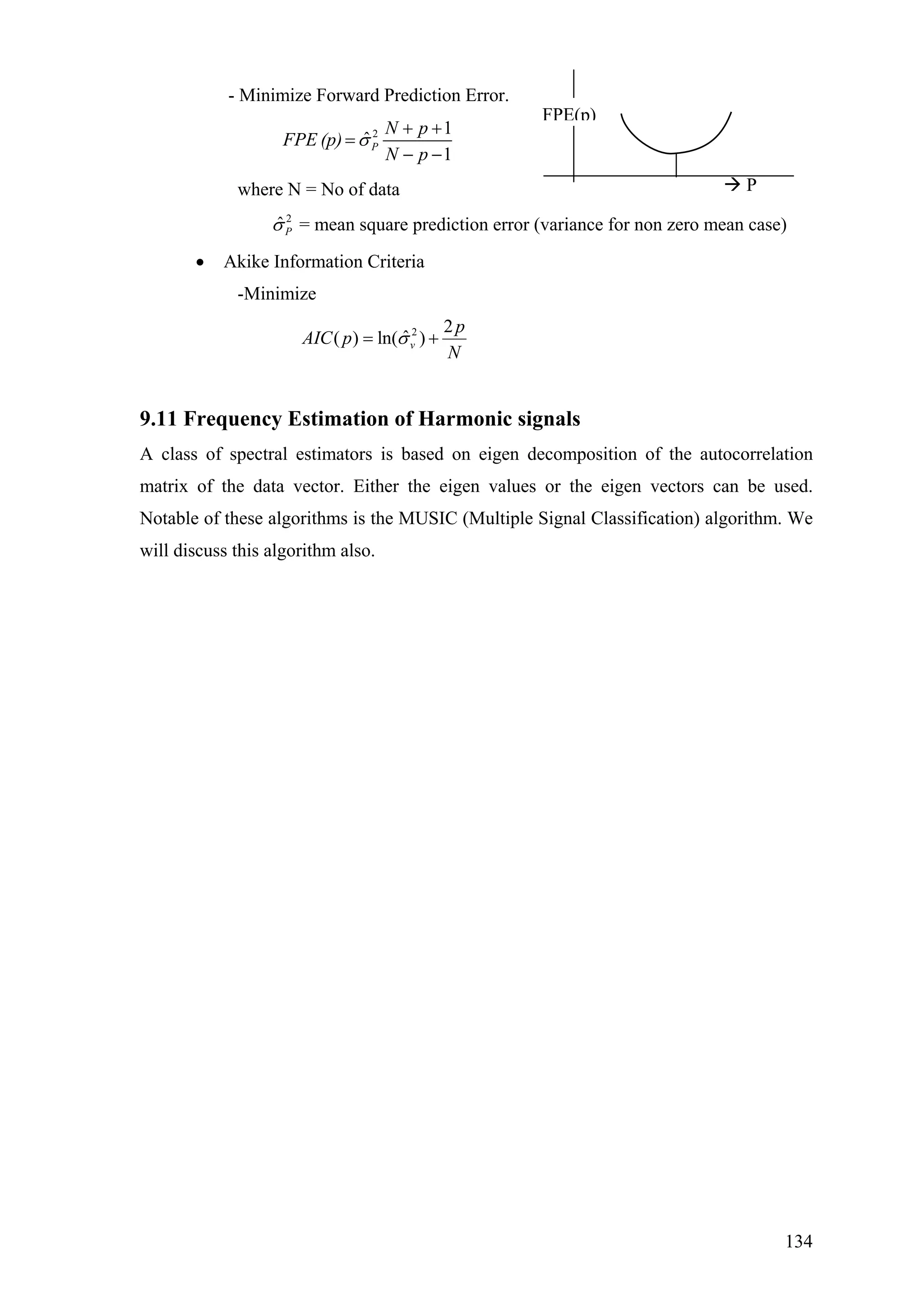


![7.13 Recursive representation of ][ˆ nYYR ...............................................................106
7.14 Matrix Inversion Lemma ..................................................................................106
7.15 RLS algorithm Steps..........................................................................................107
7.16 Discussion – RLS................................................................................................108
7.16.1 Relation with Wiener filter ............................................................................108
7.16.2. Dependence condition on the initial values..................................................109
7.16.3. Convergence in stationary condition............................................................109
7.16.4. Tracking non-staionarity...............................................................................110
7.16.5. Computational Complexity...........................................................................110
CHAPTER – 8: KALMAN FILTER ...........................................................................111
8.1 Introduction..........................................................................................................111
8.2 Signal Model.........................................................................................................111
8.3 Estimation of the filter-parameters....................................................................115
8.4 The Scalar Kalman filter algorithm...................................................................116
8.5 Vector Kalman Filter...........................................................................................117
CHAPTER – 9 : SPECTRAL ESTIMATION TECHNIQUES FOR STATIONARY
SIGNALS........................................................................................................................119
9.1 Introduction..........................................................................................................119
9.2 Sample Autocorrelation Functions.....................................................................120
9.3 Periodogram (Schuster, 1898).............................................................................121
9.4 Chi square distribution........................................................................................124
9.5 Modified Periodograms.......................................................................................126
9.5.1 Averaged Periodogram: The Bartlett Method..............................................126
9.5.2 Variance of the averaged periodogram...........................................................128
9.6 Smoothing the periodogram : The Blackman and Tukey Method .................129
9.7 Parametric Method..............................................................................................130
9.8 AR spectral estimation ........................................................................................131
9.9 The Autocorrelation method...............................................................................132
9.10 The Covariance method ....................................................................................132
9.11 Frequency Estimation of Harmonic signals ....................................................134
10. Text and Reference..................................................................................................135
7](https://crownmelresort.com/image.slidesharecdn.com/statisticalsignalprocessing1-151213044748/75/Statistical-signal-processing-1-7-2048.jpg)


![1.28 Jointly Gaussian Random variables
Two random variables are called jointly Gaussian if their joint density function
is
YX and
2 2( ) ( )( ) ( )
1
2 2 22(1 ),
2
, ( , )
x x y y
X X Y Y
XY
X YX Y X Y
X Yf x y Ae
µ µ µ µ
σ σρ σ σ
ρ
− − − −
−
⎡ ⎤
− − +⎢ ⎥
⎢ ⎥⎣ ⎦
=
where 2
,12
1
YXyx
A
ρσπσ −
=
Properties:
(1) If X and Y are jointly Gaussian, then for any constants a and then the random
variable
,b
given by is Gaussian with mean,Z bYaXZ += YXZ ba µµµ += and variance
YXYXYXZ abba ,
22222
2 ρσσσσσ ++=
(2) If two jointly Gaussian RVs are uncorrelated, 0, =YXρ then they are statistically
independent.
)()(),(, yfxfyxf YXYX = in this case.
(3) If is a jointly Gaussian distribution, then the marginal densities),(, yxf YX
are also Gaussian.)(and)( yfxf YX
(4) If X and are joint by Gaussian random variables then the optimum nonlinear
estimator
Y
Xˆ of X that minimizes the mean square error is a linear
estimator
}]ˆ{[ 2
XXE −=ξ
aYX =ˆ
25](https://crownmelresort.com/image.slidesharecdn.com/statisticalsignalprocessing1-151213044748/75/Statistical-signal-processing-1-25-2048.jpg)
![CHAPTER - 2 : REVIEW OF RANDOM PROCESS
2.1 Introduction
Recall that a random variable maps each sample point in the sample space to a point in
the real line. A random process maps each sample point to a waveform.
• A random process can be defined as an indexed family of random variables
{ ( ), }X t t T∈ whereT is an index set which may be discrete or continuous usually
denoting time.
• The random process is defined on a common probability space }.,,{ PS ℑ
• A random process is a function of the sample point ξ and index variable t and
may be written as ).,( ξtX
• For a fixed )),( 0tt = ,( 0 ξtX is a random variable.
• For a fixed ),( 0ξξ = ),( 0ξtX is a single realization of the random process and
is a deterministic function.
• When both andt ξ are varying we have the random process ).,( ξtX
The random process ),( ξtX is normally denoted by ).(tX
We can define a discrete random process [ ]X n on discrete points of time. Such a random
process is more important in practical implementations.
2( , )X t s3s
2s 1s
3( , )X t s
S
1( , )X t s
t
Figure Random Process
26](https://crownmelresort.com/image.slidesharecdn.com/statisticalsignalprocessing1-151213044748/75/Statistical-signal-processing-1-26-2048.jpg)
![2.2 How to describe a random process?
To describe we have to use joint density function of the random variables at
different .
)(tX
t
For any positive integer , represents jointly distributed
random variables. Thus a random process can be described by the joint distribution
function
n )(),.....(),( 21 ntXtXtX n
and),.....,,.....,().....,( 212121)().....(),( 21
TtNntttxxxFxxxF nnnntXtXtX n
∈∀∈∀=
Otherwise we can determine all the possible moments of the process.
)())(( ttXE xµ= = mean of the random process at .t
))()((),( 2121 tXtXEttRX = = autocorrelation function at 21,tt
))(),(),((),,( 321321 tXtXtXEtttRX = = Triple correlation function at etc.,,, 321 ttt
We can also define the auto-covariance function of given by),( 21 ttCX )(tX
)()(),(
))()())(()((),(
2121
221121
ttttR
ttXttXEttC
XXX
XXX
µµ
µµ
−=
−−=
Example 1:
(a) Gaussian Random Process
For any positive integer represent jointly random
variables. These random variables define a random vector
The process is called Gaussian if the random vector
,n )(),.....(),( 21 ntXtXtX n
n
1 2[ ( ), ( ),..... ( )]'.nX t X t X t=X )(tX
1 2[ ( ), ( ),..... ( )]'nX t X t X t is jointly Gaussian with the joint density function given by
( )
' 1
1 2
1
2
( ), ( )... ( ) 1 2( , ,... )
2 det(
X
nX t X t X t n n
e
f x x x
π
−
−
=
XC X
XC )
Ewhere '( )( )= − −X X XC X µ X µ
and [ ]1 2( ) ( ), ( )...... ( ) '.nE E X E X E X= =Xµ X
(b) Bernouli Random Process
(c) A sinusoid with a random phase.
27](https://crownmelresort.com/image.slidesharecdn.com/statisticalsignalprocessing1-151213044748/75/Statistical-signal-processing-1-27-2048.jpg)


![*
, ,( ) ( )X Y Y XS w S w=
The Wiener-Khinchin theorem is also valid for discrete-time random processes.
If we define ][][][ nXmnE XmRX +=
Then corresponding PSD is given by
[ ]
[ ] 2
( )
or ( ) 1 1
j m
X x
m
j m
X x
m
S w R m e w
S f R m e f
ω
π
π π
∞
−
=−∞
∞
−
=−∞
= −∑
= −∑
≤ ≤
≤ ≤
1
[ ] ( )
2
j m
X XR m S w e
π
ω
ππ −
dw∫∴ =
For a discrete sequence the generalized PSD is defined in the domainz − as follows
[ ]( ) m
X x
m
S z R m z
∞
−
=−∞
= ∑
If we sample a stationary random process uniformly we get a stationary random sequence.
Sampling theorem is valid in terms of PSD.
Examples 2:
2 2
2
2
(1) ( ) 0
2
( ) -
(2) ( ) 0
1
( ) -
1 2 cos
a
X
X
m
X
X
R e a
a
S w w
a w
R m a a
a
S w w
a w a
τ
τ
π π
−
= >
= ∞ < <
+
= >
−
= ≤
− +
∞
≤
)
2.6 White noise process
S (x f
→ f
A white noise process is defined by)(tX
( )
2
X
N
S f f= −∞ < < ∞
The corresponding autocorrelation function is given by
( ) ( )
2
X
N
R τ δ τ= where )(τδ is the Dirac delta.
The average power of white noise
2
avg
N
P df
∞
−∞
= →∫ ∞
32](https://crownmelresort.com/image.slidesharecdn.com/statisticalsignalprocessing1-151213044748/75/Statistical-signal-processing-1-32-2048.jpg)
![• Samples of a white noise process are uncorrelated.
• White noise is an mathematical abstraction, it cannot be realized since it has infinite
power
• If the system band-width(BW) is sufficiently narrower than the noise BW and noise
PSD is flat , we can model it as a white noise process. Thermal and shot noise are well
modelled as white Gaussian noise, since they have very flat psd over very wide band
(GHzs
• For a zero-mean white noise process, the correlation of the process at any lag 0≠τ is
zero.
• White noise plays a key role in random signal modelling.
• Similar role as that of the impulse function in the modeling of deterministic signals.
2.7 White Noise Sequence
For a white noise sequence ],[nx
( )
2
X
N
S w wπ π= − ≤ ≤
Therefore
( ) ( )
2
X
N
R m δ= m
where )(mδ is the unit impulse sequence.
White Noise WSS Random Signal
Linear
System
2.8 Linear Shi I va ia t yste ith Random Inputsft n r n S m w
Consider a discrete-time linear system with impulse response ].[nh
][][][
][][][
n* hnE xnE y
n* hnxny
=
=
For stationary input ][nx
0
[ ] [ ] [ ]
l
Y X X
k
E y n * h n h nµ µ µ
=
= = = ∑
2
N
2
N
2
N
( )XS ω
][nh
][nx
][ny
2
N
• • m• • →•
[ ]XR m
2
N
π ω→π−
33](https://crownmelresort.com/image.slidesharecdn.com/statisticalsignalprocessing1-151213044748/75/Statistical-signal-processing-1-33-2048.jpg)
![where is the length of the impulse response sequencel
][*][*][
])[*][(*])[][(
][][][
mhmhmR
mnhmnxn* hnxE
mnynE ymR
X
Y
−=
−−=
−=
is a function of lag only.][mRY m
From above we get
w)SwΗ(wS XY (|(|= 2
))
)(wSXX
Example 3:
Suppose
X
( ) 1
0 otherwise
S ( )
2
c cH w w w
N
w w
= − ≤ ≤
=
= − ∞ ≤ ≤
w
∞
Then YS ( )
2
c c
N
w w w w= − ≤ ≤
and Y cR ( ) sinc(w )
2
N
τ τ=
2
)H(w
)(wSYY
)(τXR
τ
• Note that though the input is an uncorrelated process, the output is a correlated
process.
Consider the case of the discrete-time system with a random sequence as an input.][nx
][*][*][][ mhmhmRmR XY −=
Taking the we gettransform,−z
S )()()()( 1−
= zHzHzSz XY
Notice that if is causal, then is anti causal.)(zH )( 1−
zH
Similarly if is minimum-phase then is maximum-phase.)(zH )( 1−
zH
][nh
][nx ][ny
)(zH )( 1−
zH
][mRXX
][mRYY
][zSYY( )XXS z
34](https://crownmelresort.com/image.slidesharecdn.com/statisticalsignalprocessing1-151213044748/75/Statistical-signal-processing-1-34-2048.jpg)
![Example 4:
If 1
1
( )
1
H z
zα −
=
−
and is a unity-variance white-noise sequence, then][nx
1
1
( ) ( ) ( )
1 1
1 21
YYS z H z H z
zz
1
α πα
−
−
=
⎛ ⎞⎛ ⎞
= ⎜ ⎟⎜ ⎟
−−⎝ ⎠⎝ ⎠
By partial fraction expansion and inverse −z transform, we get
||
2
1
1
][ m
Y amR
α−
=
2.9 Spectral factorization theorem
A stationary random signal that satisfies the Paley Wiener condition
can be considered as an output of a linea filter fed by a white noise
sequence.
][nX
| ln ( ) |XS w dw
π
π−
< ∞∫ r
If is an analytic function of ,)(wSX w
and , then| ln ( ) |XS w dw
π
π−
< ∞∫
2
( ) ( ) ( )X v c aS z H z H zσ=
where
)(zHc is the causal minimum phase transfer function
)(zHa is the anti-causal maximum phase transfer function
and 2
vσ a constant and interpreted as the variance of a white-noise sequence.
Innovation sequence
v n[ ] ][nX
Figure Innovation Filter
Minimum phase filter => the corresponding inverse filter exists.
)(zHc
Since is analytic in an annular region)(ln zSXX
1
zρ
ρ
< < ,
ln ( ) [ ] k
XX
k
S z c k z
∞
−
=−∞
= ∑
)
1
zHc
[ ]v n
(][nX
Figure whitening filter
35](https://crownmelresort.com/image.slidesharecdn.com/statisticalsignalprocessing1-151213044748/75/Statistical-signal-processing-1-35-2048.jpg)
![where
1
[ ] ln ( )
2
iwn
XXc k S w e dwπ
π
π −= ∫ is the order cepstral coefficient.kth
For a real signal [ ] [ ]c k c k= −
and
1
[0] ln ( )
2
XXc Sπ
π
π −= ∫ w dw
1
1
1
[ ]
[ ] [ ]
[0]
[ ]
-1 2
( )
Let ( )
1 (1)z (2) ......
k
k
k k
k k
k
k
c k z
XX
c k z c k z
c
c k z
C
c c
S z e
e e e
H z e z
h h z
ρ
∞
−
=−∞
∞ −
− −
= =−∞
∞
−
=
∑
∑ ∑
∑
−
=
=
= >
= + + +
( [0] ( ) 1c z Ch Lim H z→∞= =∵
( )CH z and are both analyticln ( )CH z
=> is a minimum phase filter.( )CH z
Similarly let
1
1
( )
( )
1
( )
1
( )
k
k
a
k
k
c k z
c k z
C
H z e
e H z z
ρ
−
−
=−∞
∞
=
∑
∑
−
=
= = <
0)
2 1
Therefore,
( ) ( ) ( )XX V C CS z H z H zσ −
=
where 2 (c
V eσ =
Salient points
• can be factorized into a minimum-phase and a maximum-phase factors
i.e. and
)(zSXX
( )CH z 1
( )CH z−
.
• In general spectral factorization is difficult, however for a signal with rational
power spectrum, spectral factorization can be easily done.
• Since is a minimum phase filter, 1
( )CH z
exists (=> stable), therefore we can have a
filter
1
( )CH z
to filter the given signal to get the innovation sequence.
• and are related through an invertible transform; so they contain the
same information.
][nX [ ]v n
36](https://crownmelresort.com/image.slidesharecdn.com/statisticalsignalprocessing1-151213044748/75/Statistical-signal-processing-1-36-2048.jpg)
![2.10 Wold’s Decomposition
Any WSS signal can be decomposed as a sum of two mutually orthogonal
processes
][nX
• a regular process [ ]rX n and a predictable process [ ]pX n , [ ] [ ] [ ]r pX n X n X n= +
• [ ]rX n can be expressed as the output of linear filter using a white noise
sequence as input.
• [ ]pX n is a predictable process, that is, the process can be predicted from its own
past with zero prediction error.
37](https://crownmelresort.com/image.slidesharecdn.com/statisticalsignalprocessing1-151213044748/75/Statistical-signal-processing-1-37-2048.jpg)
![CHAPTER - 3: RANDOM SIGNAL MODELLING
3.1 Introduction
The spectral factorization theorem enables us to model a regular random process as
an output of a linear filter with white noise as input. Different models are developed
using different forms of linear filters.
• These models are mathematically described by linear constant coefficient
difference equations.
• In statistics, random-process modeling using difference equations is known as
time series analysis.
3.2 White Noise Sequence
The simplest model is the white noise . We shall assume that is of 0-
mean and variance
[ ]v n [ ]v n
2
.Vσ
[ ]VR m
3.3 Moving Average model model)(qMA
[ ]v n ][ nX
The difference equation model is
[ ] [ ]
q
i
i o
X n b v n
=
i= −∑
2 2 2
0
0 0
and [ ] is an uncorrelated sequence means
e X
q
X i V
i
v n
b
µ µ
σ σ
=
= ⇒ =
= ∑
The autocorrelations are given by
• • • • m
FIR
filter
( )VS w 2
w
2
Vσ
π
38](https://crownmelresort.com/image.slidesharecdn.com/statisticalsignalprocessing1-151213044748/75/Statistical-signal-processing-1-38-2048.jpg)
![0 0
0 0
[ ] [ ] [ ]
[ ] [ ]
[ ]
X
q q
i j
i j
q q
i j V
i j
R m E X n X n - m
bb Ev n i v n m j
bb R m i j
= =
= =
=
= − − −∑ ∑
= − +∑ ∑
Noting that 2
[ ] [ ]V VR m σ δ= m , we get
2
[ ] when
0
V VR m
m-i j
i m j
σ=
+ =
⇒ = +
The maximum value for so thatqjm is+
2
0
[ ] 0
and
[ ] [ ]
q m
X j j m V
j
X X
R m b b m
R m R m
σ
−
+
=
= ≤∑
− =
q≤
Writing the above two relations together
2
0
[ ]
= 0 otherwise
q m
X j vj m
j
R m b b mσ
−
+
=
q= ≤∑
Notice that, [ ]XR m is related by a nonlinear relationship with model parameters. Thus
finding the model parameters is not simple.
The power spectral density is given by
2
2
( ) ( )
2
V
XS w B w
σ
π
= , where jqw
q
jw
ebebbwB −−
1 ++== ......)( ο
FIR system will give some zeros. So if the spectrum has some valleys then MA will fit
well.
3.3.1 Test for MA process
[ ]XR m becomes zero suddenly after some value of .m
[ ]XR m
m
Figure: Autocorrelation function of a MA process
39](https://crownmelresort.com/image.slidesharecdn.com/statisticalsignalprocessing1-151213044748/75/Statistical-signal-processing-1-39-2048.jpg)
![Figure: Power spectrum of a MA process
Example 1: MA(1) process
1 0
0 1
2 2 2
1 0
1 0
[ ] [ 1] [ ]
Here the parameters b and are tobe determined.
We have
[1]
X
X
X n b v n b v n
b
b b
R b b
σ
= − +
= +
=
From above can be calculated using the variance and autocorrelation at lag 1 of
the signal.
0 andb 1b
3.4 Autoregressive Model
In time series analysis it is called AR(p) model.
The model is given by the difference equation
1
[ ] [ ] [ ]
p
i
i
X n a X n i v
=
= − +∑ n
The transfer function is given by)(wA
q m→
[ ]XR m( )XS w
ω→
][nXIIR
filter
[ ]v n
40](https://crownmelresort.com/image.slidesharecdn.com/statisticalsignalprocessing1-151213044748/75/Statistical-signal-processing-1-40-2048.jpg)
![1
1
( )
1
n
j i
i
i
A w
a e ω−
=
=
− ∑
with (all poles model) and10 =a
2
2
( )
2 | ( ) |
e
XS w
A
σ
π ω
=
If there are sharp peaks in the spectrum, the AR(p) model may be suitable.
The autocorrelation function [ ]XR m is given by
1
2
1
[ ] [ ] [ ]
[ ] [ ] [ ] [ ]
[ ] [ ]
X
p
i
i
p
i X V
i
R m E X n X n - m
a EX n i X n m Ev n X n m
a R m i mσ δ
=
=
=
= − − + −∑
= − +∑
2
1
[ ] [ ] [ ]
p
X i X V
i
R m a R m i mσ δ
=
∴ = − +∑ Im ∈∨
The above relation gives a set of linear equations which can be solved to find s.ia
These sets of equations are known as Yule-Walker Equation.
Example 2: AR(1) process
1
2
1
2
1
1
1
2
2
X 2
2
2
[ ] [ 1] [ ]
[ ] [ 1] [ ]
[0] [ 1] (1)
and [1] [0]
[1]
so that
[0]
From (1) [0]
1-
After some arithmatic we get
[ ]
1-
X X V
X X V
X X
X
X
V
X
m
V
X
X n a X n v n
R m a R m m
R a R
R a R
R
a
R
R
a
a
R m
a
σ δ
σ
σ
σ
σ
= − +
= − +
∴ = − +
=
=
= =
=
ω→
( )XS ω
[ ]XR m
m→
41](https://crownmelresort.com/image.slidesharecdn.com/statisticalsignalprocessing1-151213044748/75/Statistical-signal-processing-1-41-2048.jpg)
![3.5 ARMA(p,q) – Autoregressive Moving Average Model
Under the most practical situation, the process may be considered as an output of a filter
that has both zeros and poles.
The model is given by
1 0
[ ] [ ] [ ]
p q
i i
i i
x n a X n i b v n
= =
= − +∑ ∑ i− (ARMA 1)
and is called the model.),( qpARMA
The transfer function of the filter is given by
2 2
2
( )
( )
( )
( )
( )
( ) 2
V
X
B
H w
A
B
S w
A
ω
ω
ω σ
ω π
=
=
How do get the model parameters?
For m there will be no contributions from terms to),1max( +≥ p, q ib [ ].XR m
1
[ ] [ ] max( , 1)
p
X i X
i
R m a R m i m p q
=
= − ≥ +∑
From a set of p Yule Walker equations, parameters can be found out.ia
Then we can rewrite the equation
∑ −=∴
∑ −+=
=
=
q
i
i
p
i
i
invbnX
inXanXnX
0
1
][][
~
][][][
~
From the above equation b can be found out.si
The is an economical model. Only only model may
require a large number of model parameters to represent the process adequately. This
concept in model building is known as the parsimony of parameters.
),( qpARMA )( pAR )(qMA
The difference equation of the model, given by eq. (ARMA 1) can be
reduced to
),( qpARMA
p first-order difference equation give a state space representation of the
random process as follows:
[ 1] [
[ ] [ ]
]Bu n
X n n
− +
=
z[n] = Az n
Cz
where
)(
)(
)(
wA
wB
wH =
[ ]X n
[ ]v n
42](https://crownmelresort.com/image.slidesharecdn.com/statisticalsignalprocessing1-151213044748/75/Statistical-signal-processing-1-42-2048.jpg)
![1 2
0 1
[ ] [ [ ] [ 1].... [ ]]
......
0 1......0
, [1 0...0] and
...............
0 0......1
[ ... ]
p
q
x n X n X n p
a a a
b b b
′= − −
⎡ ⎤
⎢ ⎥
⎢ ⎥ ′= =
⎢ ⎥
⎢ ⎥
⎢ ⎥⎣ ⎦
=
z n
A B
C
Such representation is convenient for analysis.
3.6 General Model building Steps),( qpARMA
• Identification of p and q.
• Estimation of model parameters.
• Check the modeling error.
• If it is white noise then stop.
Else select new values for p and q
and repeat the process.
3.7 Other model: To model nonstatinary random processes
• ARIMA model: Here after differencing the data can be fed to an ARMA
model.
• SARMA model: Seasonal ARMA model etc. Here the signal contains a
seasonal fluctuation term. The signal after differencing by step equal to the
seasonal period becomes stationary and ARMA model can be fitted to the
resulting data.
43](https://crownmelresort.com/image.slidesharecdn.com/statisticalsignalprocessing1-151213044748/75/Statistical-signal-processing-1-43-2048.jpg)


![] MAP
ˆ/ θ
MAP
ln (x) 0
θ
1ˆ
Xf
X
θ
λ
Θ
∂
=
∂
⇒ =
+
Example 8: Binary Communication problem
X is a binary random variable with
1 with probability 1/2
1 with probability 1/ 2
X
⎧
= ⎨
−⎩
V is the Gaussian noise with mean
2
0 and variance .σ
To find the MSE for X from the observed data .Y
Then
2 2
2 2
2 2 2 2
( ) / 2
/
/
/
/
( ) / 2
( 1) / 2 ( 1) / 2
1
( ) [ ( 1) ( 1)]
2
1
( / )
2
( ) ( / )
( / )
( ) ( / )
[ ( 1) ( 1)]
x
y x
Y X
X Y X
X Y
X Y X
y x
y y
f x x x
f y x e
f x f y x
f x y
f x f y x fx
e x x
e e
σ
σ
σ σ
δ δ
πσ
δ δ
− −
∞
−∞
− −
− − − +
= − + +
=
=
∫
− + +
=
+
Hence
2 2
2 2 2 2
2 2 2 2
2 2 2 2
( ) / 2
( 1) / 2 ( 1) / 2
( 1) / 2 ( 1) / 2
( 1) /2 ( 1) /2
2
[ ( 1) ( 1)]ˆ ( / )
=
tanh( / )
y x
MMSE y y
y y
y y
e x x
X E X Y x dx
e e
e e
e e
y
σ
σ σ
σ σ
σ σ
δ δ
σ
− −∞
− − − +
−∞
− − − +
− − − +
− + +
= = ∫
+
−
+
=
Y+X
V
61](https://crownmelresort.com/image.slidesharecdn.com/statisticalsignalprocessing1-151213044748/75/Statistical-signal-processing-1-61-2048.jpg)


![CHAPTER – 5: WIENER FILTER
5.1 Estimation of signal in presence of white Gaussian noise (WGN)
Consider the signal model is
][][][ nVnXnY +=
where is the observed signal, is 0-mean Gaussian with variance 1 and][nY ][nX ][nV
is a white Gaussian sequence mean 0 and variance 1. The problem is to find the best
guess for given the observation][nX [ ], 1,2,...,Y i i n=
Maximum likelihood estimation for determines that value of for which the
sequence is most likely. Let us represent the random sequence
by the random vector
][nX ][nX
[ ], 1,2,...,Y i i n=
[ ], 1,2,...,Y i i n=
[ ] [ [ ], [ 1],.., [1]]'
and the value sequence [1], [2],..., [ ] by
[ ] [ [ ], [ 1],.., [1]]'.
Y n Y n Y
y y y n
y n y n y
= −
= −
Y n
y n
The likelihood function / [ ] ( [ ]/ [ ])n X nf n x nY[ ] y will be Gaussian with mean ][nx
( )
2
1
( [ ] [ ])
2
/ [ ]
1
( [ ]/ [ ])
2
n
i
y i x n
n X n n
f n x n e
π
=
−
−∑
=Y[ ] y
Maximum likelihood will be given by
[1], [2],..., [ ]/ [ ] ˆ [ ]
( ( [1], [2],..., [ ]) / [ ]) 0
[ ] MLE
Y Y Y n X n x n
f y y y n x n
x n
∂
=
∂
1
1
ˆ [ ] [ ]
n
MLE
i
n y
n
χ
=
⇒ = ∑ i
Similarly, to find ][ˆ nMAPχ and ˆ [ ]MMSE nχ we have to find a posteriori density
2
2
1
[ ] [ ]/ [ ]
[ ]/ [ ]
[ ]
1 ( [ ] [ ])
[ ]
2 2
[ ]
( [ ]) ( [ ]/ [ ])
( [ ]/ [ ])
( [ ])
1
=
( [ ])
n
i
X n n X n
X n n
n
y i x n
x n
n
f x n f n x n
f x n
f n
e
f n
=
−
− −
=
∑
Y
Y
Y
Y
y
y n
y
y
Taking logarithm
X Y
V
+
65](https://crownmelresort.com/image.slidesharecdn.com/statisticalsignalprocessing1-151213044748/75/Statistical-signal-processing-1-65-2048.jpg)
![2
2
[ ]/ [ ] [ ]
1
1 ( [ ] [ ])
log ( [ ]) [ ] log ( [ ])
2 2
n
e X n n e n
i
y i x n
f x n x n f n
=
−
= − − −∑Y Y y
[ ]/ [ ]log ( [ ])e X n nf x nY is maximum at ˆ [ ].MAPx n Therefore, taking partial derivative of
[ ]/ [ ]log ( [ ])e X n nf x nY with respect to [ ]x n and equating it to 0, we get
1 ˆ [ ]
1
MAP
[ ] ( [ ] [ ]) 0
[ ]
ˆ [ ]
1
MAP
n
i x n
n
i
x n y i x n
y i
x n
n
=
=
− −
=
+
∑
∑
=
Similarly the minimum mean-square error estimator is given by
1
MMSE
[ ]
ˆ [ ] ( [ ]/ [ ])
1
n
i
y i
x n E X n n
n
=
= =
+
∑
y
• For MMSE we have to know the joint probability structure of the channel and the
source and hence the a posteriori pdf.
• Finding pdf is computationally very exhaustive and nonlinear.
• Normally we may be having the estimated values first-order and second-order
statistics of the data
We look for a simpler estimator.
The answer is Optimal filtering or Wiener filtering
We have seen that we can estimate an unknown signal (desired signal) [ ]x n from an
observed signal on the basis of the known joint distributions of and[ ]y n [ ]y n [ ].x n We
could have used the criteria like MMSE or MAP that we have applied for parameter es
timations. But such estimations are generally non-linear, require the computation of a
posteriori probabilities and involves computational complexities.
The approach taken by Wiener is to specify a form for the estimator that depends on a
number of parameters. The minimization of errors then results in determination of an
optimal set of estimator parameters. A mathematically sample and computationally easier
estimator is obtained by assuming a linear structure for the estimator.
66](https://crownmelresort.com/image.slidesharecdn.com/statisticalsignalprocessing1-151213044748/75/Statistical-signal-processing-1-66-2048.jpg)
![5.2 Linear Minimum Mean Square Error Estimator
The linear minimum mean square error criterion is illustrated in the above figure. The
problem can be slated as follows:
Given observations of data determine a set of
parameters such that
[ 1], [ 2].. [ ],... [ ],y n M y n M y n y n N− + − + +
[ 1], [ 2]..., [ ],... [ ]h M h M h o h N− − −
1
ˆ[ ] [ ] [ ]
M
i N
x n h i y n
−
=−
= −∑ i
and the mean square error ( )
2
ˆ[ ] [ ]E x n x n− is a minimum with respect to
[ ], [ 1]...., [ ], [ ],..., [ 1].h N h N h o h i h M− − + −
This minimization problem results in an elegant solution if we assume joint stationarity of
the signals [ ] and [ ]x n y n . The estimator parameters can be obtained from the second
order statistics of the processes [ ] and [ ].x n y n
The problem of deterring the estimator parameters by the LMMSE criterion is also called
the Wiener filtering problem. Three subclasses of the problem are identified
Noise
Filter
[ ]x n [ ]y n ˆ[ ]x n
Syste
m
+
[ 1]y n M− − …….. …[ ]y n
1n M− − n n N+
1. The optimal smoothing problem 0N >
2. The optimal filtering problem 0N =
3. The optimal prediction problem 0N <
67](https://crownmelresort.com/image.slidesharecdn.com/statisticalsignalprocessing1-151213044748/75/Statistical-signal-processing-1-67-2048.jpg)
![In the smoothing problem, an estimate of the signal inside the duration of observation of
the signal is made. The filtering problem estimates the curent value of the signal on the
basis of the present and past observations. The prediction problem addresses the issues of
optimal prediction of the future value of the signal on the basis of present and past
observations.
5.3 Wiener-Hopf Equations
The mean-square error of estimation is given by
2 2
1
2
ˆ[ ] ( [ ] [ ])
( [ ] [ ] [ ])
M
i N
Ee n E x n x n
E x n h i y n i
−
=−
= −
= − −∑
We have to minimize with respect to each to get the optimal estimation.][2
nEe ][ih
Corresponding minimization is given by
{ }2
[ ]
0, for ..0.. 1
[ ]
E e n
j N M
h j
∂
= = −
∂
−
( E being a linear operator, and
[ ]
E
h j
∂
∂
can be interchanged)
[ ] [ - ] 0, ...0,1,... 1Ee n y n j j N M= = − − (1)
or
[ ]
1
[ ] - [ ] [ ] [ - ] 0, ...0,1,... 1
a
e n
M
i N
E x n h i y n i y n j j N M
−
=−
⎛ ⎞
− = = −⎜ ⎟
⎝ ⎠
∑ −
−
(2)
1
( ) [ ] [ ], ...0,1,... 1
a
M
XY YY
i N
R j h i R j i j N M
−
=−
= − = −∑ (3)
This set of equations in (3) are called Wiener Hopf equations or Normal1N M+ +
equations.
• The result in (1) is the orthogonality principle which implies that the error is
orthogonal to observed data.
• ˆ[ ]x n is the projection of [ ]x n onto the subspace spanned by observations
[ ], [ 1].. [ ],... [ ].y n M y n M y n y n N− − + +
• The estimation uses second order-statistics i.e. autocorrelation and cross-
correlation functions.
68](https://crownmelresort.com/image.slidesharecdn.com/statisticalsignalprocessing1-151213044748/75/Statistical-signal-processing-1-68-2048.jpg)
![• If and are jointly Gaussian then MMSE and LMMSE are equivalent.
Otherwise we get a sub-optimum result.
][nx ][ny
• Also observe that
ˆ[ ] [ ] [ ]x n x n e n= +
where ˆ[ ]x n and are the parts of[ ]e n [ ]x n respectively correlated and uncorrelated
with Thus LMMSE separates out that part of[ ].y n [ ]x n which is correlated with
Hence the Wiener filter can be also interpreted as the correlation canceller. (See
Orfanidis).
[ ].y n
5.4 FIR Wiener Filter
1
0
ˆ[ ] [ ] [ ]
M
i
x n h i y n
−
=
= −∑ i
[ ] - [ ] [ ] [ - ] 0, 0,1,... 1
e n
M
i
E x n h i y n i y n j j M
−
=
⎛ ⎞
− = = −⎜ ⎟
⎝ ⎠
∑
The model parameters are given by the orthogonality principlee
[ ]
1
0
1
0
[ ] [ ] ( ), 0,1,... 1
M
YY XY
i
h i R j i R j j M
−
=
− = = −∑
In matrix form, we have
=YY XYR h r
where
[0] [ 1] .... [1 ]
[1] [0] .... [2 ]
...
[ 1] [ 2] .... [0]
YY YY YY
YY YY YY
YY YY YY
R R R M
R R R
R M R N R
− −⎡ ⎤
⎢ ⎥−⎢ ⎥=
⎢ ⎥
⎢ ⎥
− −⎢ ⎥⎣ ⎦
YYR
M
and
[0]
[1]
...
[ 1]
XY
XY
XY
R
R
R M
⎡ ⎤
⎢ ⎥
⎢ ⎥=
⎢ ⎥
⎢ ⎥
−⎢ ⎥⎣ ⎦
XYr
and
[0]
[1]
...
[ 1]
h
h
h M
⎡ ⎤
⎢ ⎥
⎢ ⎥=
⎢ ⎥
⎢ ⎥
−⎣ ⎦
h
69](https://crownmelresort.com/image.slidesharecdn.com/statisticalsignalprocessing1-151213044748/75/Statistical-signal-processing-1-69-2048.jpg)
![Therefore,
1−
= YY XYh R r
5.5 Minimum Mean Square Error - FIR Wiener Filter
1
2
0
1
0
1
0
( [ ] [ ] [ ] [ ] [ ]
= [ ] [ ] error isorthogonal to data
= [ ] [ ] [ ] [ ]
= [0] [ ] [ ]
M
i
M
i
M
XX XY
i
E e n Ee n x n h i y n i
Ee n x n
E x n h i y n i x n
R h i R i
−
=
−
=
−
=
⎛ ⎞
= − −⎜ ⎟
⎝ ⎠
⎛ ⎞
− −⎜ ⎟
⎝ ⎠
−
∑
∑
∑
∵
XX XYR r
• •
Z-1
[0]h
Z-1
Wiener
Estimation
[1]h
[ 1h M − ]
ˆ[ ]x n
70](https://crownmelresort.com/image.slidesharecdn.com/statisticalsignalprocessing1-151213044748/75/Statistical-signal-processing-1-70-2048.jpg)
![Example1: Noise Filtering
Consider the case of a carrier signal in presence of white Gaussian noise
0 0[ ] [ ],
4
[ ] [ ] [ ]
x n A cos w n w
y n x n v n
π
φ= +
= +
=
here φ is uniformly distributed in (1,2 ).π
[ ]v n is white Gaussian noise sequence of variance 1 and is independent of [ ].x n Find the
parameters for the FIR Wiener filter with M=3.
( )( )
( )
2
0
2
0
[ ] cos w
2
[ ] [ ] [ ]
[ ] [ ] [ ] [ ]
[ ] [ ] 0 0
( ) [ ]
2
[ ] [ ] [ ]
[ ] [ ] [ ]
[
XX
YY
XX VV
XY
XX
A
R m m
R m E y n y n m
E x n v m x n m v n m
R m R m
A
cos w m m
R m E x n y n m
E x n x n m v n m
R m
δ
=
= −
= + − + −
= + + +
= +
= −
= − + −
= ]
Hence the Wiener Hopf equations are
2 2 2
2 2 2
2 2 2
[0] [1] [2] [0] [0]
[1] [0] [1] [1] [1]
[2] 1] [0] [2] [2]
1 cos cos
2 2 4 2 2
cos 1 cos
2 4 2 2 4
cos cos 1
2 2 2 4 2
YY YY XX
YY YY YY XX
YY YY YY XX
R R Ryy h R
R R R h R
R R R h R
A A A
A A A
A A A
π π
π π
π π
=⎡ ⎤ ⎡ ⎤ ⎡ ⎤
⎢ ⎥ ⎢ ⎥ ⎢ ⎥
⎢ ⎥ ⎢ ⎥ ⎢ ⎥
⎢ ⎥ ⎢ ⎥ ⎢ ⎥⎣ ⎦ ⎣ ⎦ ⎣ ⎦
⎡ ⎤
+⎢ ⎥
⎢ ⎥
⎢ ⎥
+⎢
⎢
⎢ +⎢
⎣ ⎦
2
2
2
[0]
2
cos[1]
2 4
cos[2]
2 2
Ah
A
h
A
h
π
π
⎡ ⎤
⎡ ⎤ ⎢ ⎥
⎢ ⎥ ⎢ ⎥
⎢ ⎥ ⎢ ⎥
⎢ ⎥ =⎥ ⎢ ⎥
⎢ ⎥⎥ ⎢ ⎥
⎢ ⎥⎥ ⎢ ⎥
⎢ ⎥⎥ ⎢ ⎥⎣ ⎦
⎣ ⎦
suppose A = 5v then
12.5
13.5 0
12.52 [0]
12.5 12.5 12.5
13.5 [1]
2 2
[2]
12.5 0
0 13.5
2
h
h
h
⎡ ⎤
⎢ ⎥
2
⎡ ⎤
⎢ ⎥ =⎡ ⎤ ⎢ ⎥
⎢ ⎥ ⎢ ⎥ ⎢ ⎥
⎢ ⎥ ⎢ ⎥ ⎢ ⎥
⎢ ⎥ ⎢ ⎥ ⎢ ⎥⎣ ⎦
⎢ ⎥ ⎣ ⎦
⎢ ⎥
⎣ ⎦
71](https://crownmelresort.com/image.slidesharecdn.com/statisticalsignalprocessing1-151213044748/75/Statistical-signal-processing-1-71-2048.jpg)
![1
12.5
13.5 0 12.5
[0] 2
12.5 12.5 12.5
[1] 13.5
2 2
[2] 12.5
0 13.5 0
2
[0] 0.707
[1 0.34
[2] 0.226
h
h
h
h
h
h
−
⎡ ⎤
2
⎡ ⎤⎢ ⎥⎡ ⎤ ⎢ ⎥⎢ ⎥⎢ ⎥ ⎢ ⎥= ⎢ ⎥⎢ ⎥ ⎢ ⎥⎢ ⎥⎢ ⎥ ⎢ ⎥⎣ ⎦ ⎢ ⎥ ⎣ ⎦⎢ ⎥⎣ ⎦
=
=
= −
Plot the filter performance for the above values of The following
figure shows the performance of the 20-tap FIR wiener filter for noise filtering.
[0], [1] and [2].h h h
72](https://crownmelresort.com/image.slidesharecdn.com/statisticalsignalprocessing1-151213044748/75/Statistical-signal-processing-1-72-2048.jpg)
![Example 2 : Active Noise Control
Suppose we have the observation signal is given by][ny
0 1[ ] 0.5cos( ) [ ]y n w n v nφ= + +
where φ is uniformly distrubuted in ( ) 10,2 and [ ] 0.6 [ 1] [ ]v n v n v nπ = − + is an MA(1)
noise. We want to control with the help of another correlated noise given by][1 nv ][2 nv
2[ ] 0.8 [ 1] [ ]v n v n v n= − +
The Wiener Hopf Equations are given by
2 2 1 2V V V V=R h r
where [ [0] h[1]]h ′=h
and
2 2
1 2
1.64 0.8
and
0.8 1.64
1.48
0.6
V V
VV
⎡ ⎤
= ⎢ ⎥
⎣ ⎦
⎡ ⎤
= ⎢ ⎥
⎣ ⎦
R
r
[0] 0.9500
[1] -0.0976
h
h
⎡ ⎤ ⎡ ⎤
∴ =⎢ ⎥ ⎢
⎣ ⎦ ⎣
⎥
⎦
Example 3:
(Continuous time prediction) Suppose we want to predict the continuous-time process
( ) at time ( ) by
ˆ ( ) ( )
X t t
X t aX t
τ
τ
+
+ =
Then by orthogonality principle
( ( ) ( )) ( ) 0
( )
(0)
XX
XX
E X t aX t X t
R
a
R
τ
τ
+ − =
⇒ =
As a particular case consider the first-order Markov process given by
][ˆ nx][][ 1 nvnx +
2-tap FIR
filter
2[ ]v n
73](https://crownmelresort.com/image.slidesharecdn.com/statisticalsignalprocessing1-151213044748/75/Statistical-signal-processing-1-73-2048.jpg)
![( ) ( ) ( )
d
X t AX t v t
dt
= +
In this case,
( ) (0) A
XX XXR R e τ
τ −
=
( )
(0)
AXX
XX
R
a e
R
ττ −
∴ = =
Observe that for such a process
1 1
1
1 1
( ) (( )
( ( ) ( )) ( ) 0
( ) ( )
(0) (0)
0
XX XX
A AA
XX XX
E X t aX t X t
R aR
R e e R e )τ τ ττ
τ τ
τ τ τ
− + −−
+ − − =
= + −
= −
=
Therefore, the linear prediction of such a process based on any past value is same as the
linear prediction based on current value.
5.6 IIR Wiener Filter (Causal)
Consider the IIR filter to estimate the signal [ ]x n shown in the figure below.
The estimator is given by][ˆ nx
0
ˆ( ) ( ) ( )
i
x n h i y n
∞
=
= −∑ i
The mean-square error of estimation is given by
2 2
2
0
ˆ[ ] ( [ ] [ ])
( [ ] [ ] [ ])
i
Ee n E x n x n
E x n h i y n i
∞
=
= −
= − −∑
We have to minimize with respect to each to get the optimal estimation.][2
nEe ][ih
Applying the orthogonality principle, we get the WH equation.
0
0
( [ ] ( ) [ ]) [ ] 0, 0, 1, .....
From which we get
[ ] [ ] [ ], 0, 1, .....
i
YY XY
i
E x n h i y n i y n j j
h i R j i R j j
∞
=
∞
=
− − − = =
− = =
∑
∑
[ ]h n
[ ]y n ][ˆ nx
74](https://crownmelresort.com/image.slidesharecdn.com/statisticalsignalprocessing1-151213044748/75/Statistical-signal-processing-1-74-2048.jpg)
![• We have to find [ ], 0,1,...h i i = ∞ by solving the above infinite set of equations.
• This problem is better solved in the z-transform domain, though we cannot
directly apply the convolution theorem of z-transform.
Here comes Wiener’s contribution.
The analysis is based on the spectral Factorization theorem:
2 1
( ) ( ) ( )YY v c cS z H z H zσ −
=
Whitening filter
Wiener filter
Now is the coefficient of the Wiener filter to estimate2[ ]h n [ ]x n I from the innovation
sequence Applying the orthogonality principle results in the Wiener Hopf equation[ ].v n
2
0
ˆ( ) ( ) ( )
i
x n h i v n
∞
=
= −∑ i
=2
0
2
0
[ ] [ ] [ ] [ ]) 0
[ ] [ ] [ ], 0,1,...
i
VV XV
i
E x n h i v n i v n j
h i R j i R j j
∞
=
∞
=
⎧ ⎫
− − −⎨ ⎬
⎩ ⎭
∴ − = =
∑
∑
2
2
2
0
[ ] [ ]
( ) [ ] ( ), 0,1,...
VV V
V XV
i
R m m
h i j i R j j
σ δ
σ δ
∞
=
=
∴ − = =∑
So that
[ ]
2 2
2 2
[ ]
[ ] j 0
( )
( )
XV
V
XV
V
R j
h j
S z
H z
σ
σ
= ≥
+
=
where [ ]( )XVS z + is the positive part (i.e., containing non-positive powers of ) in power
series expansion of
z
( ).XVS z
[ ]v n[ ]y n
1
1
( )cH z
( )H z =
[ ]v n
2 ( )H z
][ˆ nx
1( )H Z
[ ]y n
75](https://crownmelresort.com/image.slidesharecdn.com/statisticalsignalprocessing1-151213044748/75/Statistical-signal-processing-1-75-2048.jpg)
![1
0
0
1
0
1
1 1
2 2 1
[ ] [ ] [ ]
[ ] [ ] [ ]
[ ] [ ] [ - - ]
[ ] [j i]
1
( ) ( ) ( ) ( )
( )
( )1
( )
( )
i
XV
i
i
XY
i
XV XY XY
c
XY
V c
v n h i y n i
R j Ex n v n j
h i E x n y n j i
h i R
S z H z S z S z
H z
S z
H z
H zσ
∞
=
∞
=
∞
=
−
−
−
+
= −
= −
=
= +
= =
⎡ ⎤
∴ = ⎢ ⎥
⎣ ⎦
∑
∑
∑
Therefore,
1 2 2 1
1 (
( ) ( ) ( )
( ) ( )
XY
V c c
S z
H z H z H z
H z H zσ −
)
+
⎡ ⎤
= = ⎢ ⎥
⎣ ⎦
We have to
• find the power spectrum of data and the cross power spectrum of the of the
desired signal and data from the available model or estimate them from the data
• factorize the power spectrum of the data using the spectral factorization theorem
5.7 Mean Square Estimation Error – IIR Filter (Causal)
2
0
0
0
( [ ] [ ] [ ] [ ] [ ]
= [ ] [ ] error isorthogonal to data
= [ ] [ ] [ ] [ ]
= [0] [ ] [ ]
i
i
XX XY
i
E e n Ee n x n h i y n i
Ee n x n
E x n h i y n i x n
R h i R i
∞
=
∞
=
∞
=
⎛ ⎞
= − −⎜ ⎟
⎝ ⎠
⎛ ⎞
− −⎜ ⎟
⎝ ⎠
−
∑
∑
∑
∵
*
*
1 1
1 1
( ) ( ) ( )
2 2
1
( ( ) ( ) ( ))
2
1
( ( ) ( ) ( ))
2
X X
X XY
X XY
C
S w dw H w S w dw
S w H w S w dw
S z H z S z z dz
π π
π π
π
π
π π
π
π
− −
−
− −
= −
= −
= −
∫ ∫
∫
∫
Y
76](https://crownmelresort.com/image.slidesharecdn.com/statisticalsignalprocessing1-151213044748/75/Statistical-signal-processing-1-76-2048.jpg)
![Example 4:
1[ ] [ ] [ ]y n x n v n= + observation model with
[ ] 0.8 [ -1] [ ]x n x n w= + n
where v n is and additive zero-mean Gaussian white noise with variance 1 and
is zero-mean white noise with variance 0.68. Signal and noise are uncorrelated.
1[ ] [ ]w n
Find the optimal Causal Wiener filter to estimate [ ].x n
Solution:
( )( )1
0.68
( )
1 0.8 1 0.8
XXS z
z z−
=
− −
( )(
[ ] [ ] [ ]
[ ] [ ] [ ] [ ]
[ ] [ ] 0 0
( ) ( ) 1
YY
XX VV
YY XX
R m E y n y n m
)E x n v m x n m v n m
R m R m
S z S z
= −
= + − + −
= + + +
= +
Factorize
( )( )
( )( )
( )
1
1
1
1
1
2
0.68
( ) 1
1 0.8 1 0.8
2(1 0.4 )(1 0.4 )
=
1 0.8 1 0.8
(1 0.4 )
( )
1 0.8
2
YY
c
V
S z
z z
z z
z z
z
H z
z
and
σ
−
−
−
−
−
= +
− −
− −
− −
−
∴ =
−
=
Also
( )(
( )( )
)
1
[ ] x[ ] [ ]
[ ] [ ] [ ]
[ ]
( ) ( )
0.68
=
1 0.8 1 0.8
XY
XX
XY XX
R m E n y n m
E x n x n m v n m
R m
S z S z
z z−
= −
= − +
=
=
− −
−
1
1
1 0.8z−
−
[ ]w n [ ]x n
77](https://crownmelresort.com/image.slidesharecdn.com/statisticalsignalprocessing1-151213044748/75/Statistical-signal-processing-1-77-2048.jpg)
![( )
( )
2 1
1
11
1
( )1
( )
( ) ( )
1 0.68(1 0.8 )
=
2 (1 0.8 )(1 0.8 )1 0.4
0.944
=
1 0.4
[ ] 0.944(0.4) 0
XY
V c c
n
S z
H z
H z H z
z
z zz
z
h n n
σ −
+
−
−−
+
−
⎡ ⎤
∴ = ⎢ ⎥
⎣ ⎦
⎡ ⎤−
⎢ ⎥
− −− ⎣ ⎦
−
= ≥
5.8 IIR Wiener filter (Noncausal)
The estimator is given by][ˆ nx
∑−=
−=
α
αi
inyihnx ][][][ˆ
For LMMSE, the error is orthogonal to data.
[ ] [ ] [ ] [ ] 0 j I
i
E x n h i y n i y n j
α
α=−
⎛ ⎞
− − − =⎜ ⎟
⎝ ⎠
∑ ∀ ∈
[ ] [ ] [ ], ,...0, 1, ...YY XY
i
h i R j i R j j
∞
=−∞
− = = −∞ ∞∑
[ ]y n ][ˆ nx
( )H z
• This form Wiener Hopf Equation is simple to analyse.
• Easily solved in frequency domain. So taking Z transform we get
• Not realizable in real time
( ) ( ) ( )YY XYH z S z S z=
so that
( )
( )
( )
or
( )
( )
( )
XY
YY
XY
YY
S z
H z
S z
S w
H w
S w
=
=
78](https://crownmelresort.com/image.slidesharecdn.com/statisticalsignalprocessing1-151213044748/75/Statistical-signal-processing-1-78-2048.jpg)
![5.9 Mean Square Estimation Error – IIR Filter (Noncausal)
The mean square error of estimation is given by
2
( [ ] [ ] [ ] [ ] [ ]
= [ ] [ ] error isorthogonal to data
= [ ] [ ] [ ] [ ]
= [0] [ ] [ ]
i
i
XX XY
i
E e n Ee n x n h i y n i
Ee n x n
E x n h i y n i x n
R h i R i
∞
=−∞
∞
=−∞
∞
=−∞
⎛ ⎞
= − −⎜ ⎟
⎝ ⎠
⎛ ⎞
− −⎜ ⎟
⎝ ⎠
−
∑
∑
∑
∵
*1 1
( ) ( ) ( )
2 2
X XS w dw H w S w dw
π π
π π Y
π π− −
= −∫ ∫
*
1 1
1
( ( ) ( ) ( ))
2
1
( ( ) ( ) ( ))
2
X XY
X XY
C
S w H w S w dw
S z H z S z z dz
π
ππ
π
−
− −
= −
= −
∫
∫
Example 5: Noise filtering by noncausal IIR Wiener Filter
Consider the case of a carrier signal in presence of white Gaussian noise
[ ] [ ] [ ]y n x n v n= +
where is and additive zero-mean Gaussian white noise with variance[ ]v n 2
.Vσ Signal
and noise are uncorrelated
( ) ( ) ( )
and
( ) ( )
( )
( )
( ) ( )
( )
( )
=
(
) 1
( )
YY XX VV
XY XX
XX
XX VV
XY
VV
XX
VV
S w S w S w
S w S w
S w
H w
S w S w
S w
S w
S w
S w
= +
=
∴ =
+
+
Suppose SNR is very high
( ) 1H w ≅
(i.e. the signal will be passed un-attenuated).
When SNR is low
( )
( )
( )
XX
VV
S w
H w
S w
=
79](https://crownmelresort.com/image.slidesharecdn.com/statisticalsignalprocessing1-151213044748/75/Statistical-signal-processing-1-79-2048.jpg)
![(i.e. If noise is high the corresponding signal component will be attenuated in proportion
of the estimated SNR.
Figure - (a) a high-SNR signal is passed unattended by the IIR Wiener filter
(b) Variation of SNR with frequency
Example 6: Image filtering by IIR Wiener filter
( ) power spectrum of the corrupted image
( ) power spectrum of the noise, estimated from the noise model
or from the constant intensity ( like back-ground) of the image
( )
( )
YY
VV
XX
S w
S w
S w
H w
S
=
=
=
( ) ( )
( ) ( )
=
( )
XX VV
YY VV
YY
w S w
S w S w
S w
+
−
Example 7:
Consider the signal in presence of white noise given by
[ ] 0.8 [ -1] [ ]x n x n w= + n
where v n is and additive zero-mean Gaussian white noise with variance 1 and
is zero-mean white noise with variance 0.68. Signal and noise are uncorrelated.
[ ] [ ]w n
Find the optimal noncausal Wiener filter to estimate [ ].x n
( )H w
SNR
Signal
Noise
w
80](https://crownmelresort.com/image.slidesharecdn.com/statisticalsignalprocessing1-151213044748/75/Statistical-signal-processing-1-80-2048.jpg)
![( )( )
( )( )
( )( )
( )( )
-1
XY
-1
YY
-1
-1
-1
0.68
1-0.8z 1 0.8zS ( )
( )
S ( ) 2 1-0.4z 1 0.4z
1-0.6z 1 0.6z
0.34
One pole outside the unit circle
1-0.4z 1 0.4z
0.4048 0.4048
1-0.4z 1-0.4z
[ ] 0.4048(0.4) ( ) 0.4048(0.4) (n n
z
H z
z
h n u n u−
−
= =
−
−
=
−
= +
∴ = + − 1)n −
[ ]h n
n
Figure - Filter Impulse Response
81](https://crownmelresort.com/image.slidesharecdn.com/statisticalsignalprocessing1-151213044748/75/Statistical-signal-processing-1-81-2048.jpg)
![CHAPTER – 6: LINEAR PREDICTION OF SIGNAL
6.1 Introduction
Given a sequence of observation
what is the best prediction for[ 1] [ 2], [ ],y n- , y n- . y n- M… [ ]?y n
(one-step ahead prediction)
The minimum mean square error prediction for is given byˆ[ ]y n [ ]y n
{ }ˆ [ ] [ ] [ 1] [ 2] [ ]y n E y n | y n - , y n - ,...,y n - M= which is a nonlinear predictor.
A linear prediction is given by
∑=
−=
M
i
inyihny
1
][][][ˆ
where are the prediction parameters.Miih ....1],[ =
• Linear prediction has very wide range of applications.
• For an exact AR (M) process, linear prediction model of order M and the
corresponding AR model have the same parameters. For other signals LP model gives
an approximation.
6.2 Areas of application
• Speech modeling • ECG modeling
• Low-bit rate speech coding • DPCM coding
• Speech recognition • Internet traffic prediction
LPC (10) is the popular linear prediction model used for speech coding. For a frame of
speech samples, the prediction parameters are estimated and coded. In CELP (Code book
Excited Linear Prediction) the prediction error ˆ[ ] [ ]- [ ]e n y n y n= is vector quantized and
transmitted.
M
i 1
ˆ [ ] [ ] [ ]y n h i y n -i
=
= ∑ is a FIR Wiener filter shown in the following figure. It is called
the linear prediction filter.
82](https://crownmelresort.com/image.slidesharecdn.com/statisticalsignalprocessing1-151213044748/75/Statistical-signal-processing-1-82-2048.jpg)
![Therefore
M
i 1
ˆ[ ] y[ ]- [ ]
[ ] [ ] [ ]
e n n y n
y n h i y n -i
=
=
= − ∑
is the prediction error and the corresponding filter is called prediction error filter.
Linear Minimum Mean Square error estimates for the prediction parameters are given by
the orthogonality relation
M
i 1
M
i 1
M
i 1
[ ] [ ] 0 1 2
( [ ] [ ] [ ])y[ ] 0 1 2
[ ] [ ] [ ] 0
[ ] [ ] [ ] 1 2
YY YY
YY YY
E e n y n - j = for j= , ,…,M
E y n h i y n -i n j j= , ,…,M
R j - h i R j -i =
R j h i R j -i j= , ,…,M
=
=
=
∴ − − =
⇒
⇒ =
∑
∑
∑
which is the Wiener Hopf equation for the linear prediction problem and same as the Yule
Walker equation for AR (M) Process.
In Matrix notation
[0] [1] .... [ 1] [1][1]
[1] [ ] ... [ - 2] [2][2]
.. .
.. .
.. .
[ ][ -1] [ - 2] ...... [0] [ ]
YY YY YY YY
YY YY YY YY
YY YY YY YY
R R R M Rh
R R o R M Rh
h MR M R M R R M
−⎡ ⎤ ⎡ ⎤
⎢ ⎥ ⎢ ⎥
⎢ ⎥ ⎢ ⎥
⎢ ⎥ ⎢ ⎥
=⎢ ⎥ ⎢ ⎥
⎢ ⎥ ⎢ ⎥
⎢ ⎥ ⎢ ⎥
⎢ ⎥ ⎢ ⎥
⎢ ⎥⎢ ⎥ ⎣ ⎦⎣ ⎦
⎥
⎥
⎥
⎡ ⎤
⎢ ⎥
⎢ ⎥
⎢ ⎥
⎢ ⎥
⎢ ⎥
⎢
⎢
⎢⎣ ⎦
YYYY
YYYY
rRh
rhR
1
)( −
=∴
=
6.3 Mean Square Prediction Error (MSPE)
∑
∑
∑
=
=
=
−=
−−=
=
−−=
M
i
YYYY
M
i
M
i
iRihR
inyihnynEy
nenEy
neinyihnyEneE
1
1
1
2
])[][]0[
])[][][]([
][][
][])[][][(])[(
83](https://crownmelresort.com/image.slidesharecdn.com/statisticalsignalprocessing1-151213044748/75/Statistical-signal-processing-1-83-2048.jpg)
![6.4 Forward Prediction Problem
The above linear prediction problem is the forward prediction problem. For notational
simplicity let us rewrite the prediction equation as
M
i 1
ˆ [ ] [ ] [ ]My n h i y n -i
=
= ∑
where the prediction parameters are being denoted by ....1],[ MiihM =
6.5 Backward Prediction Problem
Given we want to estimate .[ ] [ 1], [ 1],y n , y n- . y n- M… + y n M[ ]−
The linear prediction is given by
M
i 1
ˆy[ ] [ ] y[ 1 ]]Mn- M b i n i
=
= +∑ −
.
.
.
⎡ ⎤
⎢
Applying orthogonality principle.
1
( [ - ]- [ ] [ 1 ]) [ 1 ] 0 1,2..., .
M
M
i
E y n M b i y n i y n j j M
=
+ − + − = =∑
This will give
, …, M,j =j-iRibjMR YYMYY 21][][]1[
M
1i
∑=−+
=
Corresponding matrix form
[0] [1] .... [ 1] [1] [ ]
[1] [ ] ... [ - 2] [2] [ 1]
. .
. .
. .
[ -1] [ - 2] ...... [0] [ ] [1]
YY YY YY M YY
YY YY YY M YY
YY YY YY M YY
R R R M b R M
R R o R M b R M
R M R M R b M R
−⎡ ⎤ ⎡ ⎤
⎢ ⎥ ⎢ ⎥ −⎢ ⎥ ⎢ ⎥
⎢ ⎥ ⎢ ⎥
=⎢ ⎥ ⎢ ⎥
⎢ ⎥ ⎢ ⎥
⎢ ⎥ ⎢ ⎥
⎢ ⎥ ⎢ ⎥
⎢ ⎥ ⎢ ⎥⎣ ⎦ ⎣ ⎦
⎢
⎢
⎢
⎢
⎢
⎢
⎢⎣ ⎦
⎥
⎥
⎥
⎥
⎥
⎥
⎥
⎥
(1)
6.6 Forward Prediction
Rewriting the Mth-order forward prediction problem, we have
[0] [1] .... [ 1] [1] [1]
[1] [ ] ... [ -2] [2] [2
. .
. .
. .
[ -1] [ - 2] ...... [0] [ ]
YY YY YY M YY
YY YY YY M YY
YY YY YY M
R R R M h R
R R o R M h R
R M R M R h M
−⎡ ⎤ ⎡ ⎤
⎢ ⎥ ⎢ ⎥
⎢ ⎥ ⎢ ⎥
⎢ ⎥ ⎢ ⎥
=⎢ ⎥ ⎢ ⎥
⎢ ⎥ ⎢ ⎥
⎢ ⎥ ⎢ ⎥
⎢ ⎥ ⎢ ⎥
⎢ ⎥ ⎢ ⎥⎣ ⎦ ⎣ ⎦
]
.
.
.
[ ]YYR M
⎡ ⎤
⎢ ⎥
⎢ ⎥
⎢ ⎥
⎢ ⎥
⎢ ⎥
⎢ ⎥
⎢ ⎥
⎢ ⎥⎣ ⎦
(2)
From (1) and (2) we conclude
84](https://crownmelresort.com/image.slidesharecdn.com/statisticalsignalprocessing1-151213044748/75/Statistical-signal-processing-1-84-2048.jpg)
![MiiMhib MM ...,2,1],1[][ =−+=
Thus forward prediction parameters in reverse order will give the backward prediction
parameters.
M S prediction error
∑
∑
∑
=
=
=
−+−+−=
−+−=
−⎟
⎠
⎞
⎜
⎝
⎛
−+−−=
M
i
YYMYY
M
i
YYMYY
M
i
MM
iMRiMhR
iMRibR
MnyinyibMnyE
1
1
1
]1[]1[]0[
]1[][]0[
][]1[][][ε
which is same as the forward prediction error.
Thus
Example 1:
Backward prediction error = Forward Prediction error.
Find the second order predictor for given][ny [ ] [ ] [ ],y n x n v n= + where is a 0-mean
white noise with variance 1 and uncorrelated with and
][nv
][nx [ ] 0 8 [ 1] [ ]x n . x n- w n= + ,
is a 0-mean random variable with variance 0.68[ ]w n
The linear predictor is given by
22
ˆ [ ] [ ] [ ] [2] [ 2]1 1y h y h y nn n −= − +
We have to find hh ].2[and]1[ 22
Corresponding Yule Walker equations are
⎥
⎦
⎤
⎢
⎣
⎡
=⎥
⎦
⎤
⎢
⎣
⎡
⎥
⎦
⎤
⎢
⎣
⎡
[2]
[1]
YY
YY
YYYY
YYYY
R
R
h
h
RR
RR
]2[
]1[
]0[]1[
]1[]0[
2
2
To find out ]2[and]1[,]0[ YYYYYY RRR
[ ] [ ] [ ],
[ ] [ ] [ ]YY XX
y n x n v n
R m R m mδ
= +
= +
| || |
2
[ ] 0 8 [ 1] [ ]
0.68
[ ] 8 9 8(0. ) 1.8 (0. )
1 (0.8)
[0] 2.89, [1] 1.51 and [2] 1.21
mm
XX
YY YY YY
x n . x n - w n
R m
R R R
= +
∴ = = ×
−
= = =
Solving 2 2[1] 0.4178 and h [2] 0.2004.h = =
85](https://crownmelresort.com/image.slidesharecdn.com/statisticalsignalprocessing1-151213044748/75/Statistical-signal-processing-1-85-2048.jpg)
![6.7 Levinson Durbin Algorithm
Levinson Durbin algorithm is the most popular technique for determining the LPC
parameters from a given autocorrelation sequence.
Consider the Yule Walker equation for order linear predictor.mth
[m]
.
.
.
.
[1]
][
.
.
.
]2[
]1[
]0[]1[
]2[.][]1[
]1[]1[]0[
m
m
m
⎥
⎥
⎥
⎥
⎥
⎥
⎥
⎦
⎤
⎢
⎢
⎢
⎢
⎢
⎢
⎢
⎣
⎡
=
⎥
⎥
⎥
⎥
⎥
⎥
⎥
⎦
⎤
⎢
⎢
⎢
⎢
⎢
⎢
⎢
⎣
⎡
⎥
⎥
⎥
⎥
⎥
⎥
⎥
⎥
⎦
⎤
⎢
⎢
⎢
⎢
⎢
⎢
⎢
⎢
⎣
⎡ −
YY
YY
YYYY
yyYYYY
YYYYYY
R
R
mh
h
h
R......m-R
.
.
.
m-R...oRR
m.... RRR
(1)
Writing in the reverse order
[1]
.
.
.
.
[m]
]1[
.
.
.
]1[
][
]0[]1[
]2[.][]1[
]1[]1[]0[
m
m
m
⎥
⎥
⎥
⎥
⎥
⎥
⎥
⎦
⎤
⎢
⎢
⎢
⎢
⎢
⎢
⎢
⎣
⎡
=
⎥
⎥
⎥
⎥
⎥
⎥
⎥
⎦
⎤
⎢
⎢
⎢
⎢
⎢
⎢
⎢
⎣
⎡
−
⎥
⎥
⎥
⎥
⎥
⎥
⎥
⎥
⎦
⎤
⎢
⎢
⎢
⎢
⎢
⎢
⎢
⎢
⎣
⎡ −
YY
YY
YYYY
yyYYYY
YYYYYY
R
R
h
mh
mh
R......m-R
.
.
.
m-R...oRR
m.... RRR
(2)
Then (m+1) the order predictor is given by
[0] [1] [ 1] [ ]
[1] [0] [ 2] [ 1]
[ 1] [ 2] [0] [1]
[ ]
YY YY YY YY
YY YY YY YY
YY YY YY YY
YY
R R .... R m R m
R R .... R m R m
.
.
.
R m R m .... R R
R m
−
− −
− −
m 1
m 1
1 YY
YY1
[1] [1]
[2] [2]
. .
. .
. .
[ ] [m]
[ 1] [1] [0] [m 1][ 1]
YY
YY
m
YY YY YY m
h R
h R
h m R
R m .... R R Rh m
+
+
+
+
⎡ ⎤ ⎡
⎢ ⎥ ⎢
⎢ ⎥ ⎢
⎢ ⎥ ⎢
⎢ ⎥ ⎢
=⎢ ⎥ ⎢
⎢ ⎥ ⎢
⎢ ⎥ ⎢
⎢ ⎥ ⎢
⎤ ⎡ ⎤
⎥ ⎢ ⎥
⎥ ⎢ ⎥
⎥ ⎢ ⎥
⎥ ⎢ ⎥
⎥ ⎢ ⎥
⎥ ⎢ ⎥
⎥ ⎢ ⎥
⎥ ⎢ ⎥
⎥ ⎢ ⎥− ++⎢ ⎥ ⎢ ⎥ ⎢ ⎥⎣ ⎦ ⎣ ⎦ ⎣ ⎦
⎢ ⎥ ⎢
Let us partition equation (2) as shown. Then
(3)
][
.
.
.
[2]
[1]
]1[
.
.
.
1]-[m
[m]
1][mh
][
.
.
.
]2[
]1[
]0[]2[]1[
]2[]0[]1[
]1[]1[]0[
1m
1
1m
1m
⎥
⎥
⎥
⎥
⎥
⎥
⎥
⎦
⎤
⎢
⎢
⎢
⎢
⎢
⎢
⎢
⎣
⎡
=
⎥
⎥
⎥
⎥
⎥
⎥
⎥
⎦
⎤
⎢
⎢
⎢
⎢
⎢
⎢
⎢
⎣
⎡
++
⎥
⎥
⎥
⎥
⎥
⎥
⎥
⎦
⎤
⎢
⎢
⎢
⎢
⎢
⎢
⎢
⎣
⎡
⎥
⎥
⎥
⎥
⎥
⎥
⎦
⎤
⎢
⎢
⎢
⎢
⎢
⎢
⎣
⎡
−−
−
−
+
+
+
+
mR
R
R
R
R
R
mh
h
h
R....mRmR
.
.
mR....RR
mR....RR
YY
YY
YY
YY
YY
YY
m
YYYYYY
YYYYYY
YYYYYY
and
1 1
1
[ ] [ 1 ] [ 1] [0] [ 1]
m
m YY m YY YY
i
h i R m i h m R R m+ +
=
+ − + + = +∑ (4)
86](https://crownmelresort.com/image.slidesharecdn.com/statisticalsignalprocessing1-151213044748/75/Statistical-signal-processing-1-86-2048.jpg)
![From equation (3) premultiplying by we get,1
YYR−
][
.
.
.
[2]
[1]
]1[
.
.
.
1]-[m
[m]
1][mh
][
.
.
.
]2[
]1[
1m
1
1m
1m
⎥
⎥
⎥
⎥
⎥
⎥
⎥
⎦
⎤
⎢
⎢
⎢
⎢
⎢
⎢
⎢
⎣
⎡
=
⎥
⎥
⎥
⎥
⎥
⎥
⎥
⎦
⎤
⎢
⎢
⎢
⎢
⎢
⎢
⎢
⎣
⎡
++
⎥
⎥
⎥
⎥
⎥
⎥
⎥
⎦
⎤
⎢
⎢
⎢
⎢
⎢
⎢
⎢
⎣
⎡
−−
+
+
+
+
mR
R
R
R
R
R
mh
h
h
YY
YY
YY
YY
YY
YY
m
1
YY
1
YY RR
⎥
⎥
⎥
⎥
⎥
⎥
⎥
⎦
⎤
⎢
⎢
⎢
⎢
⎢
⎢
⎢
⎣
⎡
=
⎥
⎥
⎥
⎥
⎥
⎥
⎥
⎦
⎤
⎢
⎢
⎢
⎢
⎢
⎢
⎢
⎣
⎡
−
++
⎥
⎥
⎥
⎥
⎥
⎥
⎥
⎦
⎤
⎢
⎢
⎢
⎢
⎢
⎢
⎢
⎣
⎡
=
+
+
+
+
][
.
.
.
]2[
])1[
]1[
.
.
.
]1[
][
1][m
][
.
.
.
]2[
]1[
m
m
m
m
m
1
1m
1m
1m
mh
h
h
h
mh
mh
h
mh
h
h m
m
The equations can be rewritten as
miimhkihih mmmm ,...2,1]1[][][ 11 =−++= ++ (5)
where is called the reflection coefficient or the PARCOR (partial
correlation) coefficient.
][mhk mm −=
From equation (4) we get
]1[]0[][]1[][
1
11 +=∑ +−+
=
++ mRRmhimRih YY
m
i
YYmYYm
using equation (5)
error.predictionsquare-meantheis]1[]1[]0[][
where
][
]1[][
][
]1[][]1[
]1[][]1[}]1[]1[]0[{
]1[]1[]1[]0[]1[][
]1[]0[]1[}]1[][{
1
0
1
1
11
1
1
1
1
1
1
11
∑
∑
∑
∑∑
∑∑
∑
=
=
=
+
==
+
=
+
=
+
=
++
−+−+−=
−+
=
−+++−
=
−+++−=−+−+−
+=−+−++−−+
+=−−+−++
m
i
YYmYY
m
i
YYm
m
i
YYmYY
m
m
i
YYmYY
m
i
YYmYYm
YY
m
i
YYmm
m
i
YYmYYm
YY
m
i
YYmYYmmm
imRimhRm
m
imRih
m
imRihmR
k
imRihmRimRimhRk
mRimRimhkRkimRih
mRRkimRimhkih
ε
ε
ε
87](https://crownmelresort.com/image.slidesharecdn.com/statisticalsignalprocessing1-151213044748/75/Statistical-signal-processing-1-87-2048.jpg)
![1]0[thatassumptiontheusedhaveweHere −=mh
]2[]2[]0[]1[
1
1
1∑ −+−+−=+∴
+
=
+
m
i
YYmYY imRimhRmε
Using the recursion for ][1 ihm+
We get
( )2
11][]1[ +−=+ mkmm εε
will give MSE recursively. Since MSE is non negative
1
12
≤∴
≤
m
m
k
k
• If 1,mk < the LPC error filter will be minimum-phase, and hence the corresponding
syntheses filter will be stable.
• Efficient realization can be achieved in terms of .mk
• represents the direct correlation of the datamk [ ]y n m− on when the
correlation due to the intermediate data
[ ]y n
[ 1], [ 2],..., [ 1]y n m y n m y n− + − + − is
removed. It is defined by
[ ] [ ]
(0)
f f
m m
m
yy
Ee n e n
k
R
=
where
1
1
[ ] forward prediction error = [ ] [ ] [ ]
and
[ ] backward prediction error= [ ] [ 1 ] [ 1 ]
n
f
m m
i
n
b
m m
i
e n y n h i y n i
e n y n m h m i y n i
=
=
= − −
= − − +
∑
∑ − + −
6.8 Steps of the Levinson- Durbin algorithm
Given .2,1,0,,][ …=mmRYY
Initialization
Take mhm allfor1]0[ −=
For ,0=m
]0[]0[ YYR=ε
For ...3,2,1=m
1
1
0
[ ] [ ]
[ 1]
m
m YY
i
m
h i R m i
k
mε
−
−
=
−
=
−
∑
88](https://crownmelresort.com/image.slidesharecdn.com/statisticalsignalprocessing1-151213044748/75/Statistical-signal-processing-1-88-2048.jpg)
![1-m1,2...,i,][][][ 11 =−+= −− imhkihih mmmm
)1(
][
2
1 mmm
mm
k
kmh
−=
−=
−εε
Go on computing up to given final value of .m
Some salient points
• The reflection parameters and the mean-square error completely determine the LPC
coefficients. Alternately, given the reflection coefficients and the final mean-square
prediction error, we can determine the LPC coefficients.
• The algorithm is order recursive. By solving for order linear prediction problem
we get all previous order solutions
-m th
• If the estimated autocorrelation sequence satisfy the properties of an autocorrelation
functions, the algorithm will yield stable coefficients
6.9 Lattice filer realization of Linear prediction error filters
[ ] = prediction error due to order forward prediction.
[ ] = prediction error due to order backward prediction.
f
m
b
m
e n mth
e n mth
Then,
1
[ ] = [ ] [ ] [ ]
m
f
m m
i
e n y n h i y n i
=
− ∑ −
+ −
(1)
1
[ ] [ - ]- [ 1 ] [ 1 ]
m
b
m m
i
e n y n m h m i y n i
=
= + −∑
From (1), we get
( )
]1[][
][][][][][][
][][][][][
][][][][][][
11
1
1
1
1
1
1
1
1
11
1
1
−+=
⎟
⎠
⎞
⎜
⎝
⎛
−−−−+−−=
−−+−−+=
−−−−=
−−
−
=
−
−
=
−
−
=
−−
−
=
∑∑
∑
∑
nekne
inyimhmnykinyihny
inyimhkihmnykny
inyihmnymhnyne
mm
f
m
m
i
mm
m
i
m
m
i
mmmm
m
i
mm
f
m
1 1[ ] [ ] [ 1]f f b
m m m me n e n k e n− −∴ = + −
Similarly we can show that
1 1[ ] [ 1] [ ]b b f
m m m me n e n k e n− −= − +
89](https://crownmelresort.com/image.slidesharecdn.com/statisticalsignalprocessing1-151213044748/75/Statistical-signal-processing-1-89-2048.jpg)
![mk
mk
1
z−
1[ ]f
me n−
1[ ]b
me n−
+
+
[ ]f
me n
[ ]b
me n
How to initialize the lattice?
We have
0][
0][
0
0
−=
−=
nye
and
nye
b
f
Hence
0 0
[ ]f be e y n= = +
+1
z−
[ ]y n
1k
1k
6.10 Advantage of Lattice Structure
• Modular structure can be extended by first cascading another section. New stages
can be added without modifying the earlier stages.
• Same elements are used in each stage. So efficient for VLSI implementation.
• Numerically efficient as |km| < 1.
• Each stage is decoupled with earlier stages.
=> It follows from the fact that for W.S.S. signal, sequences as a function of m are
uncorrelated.
[ ]me n
[ ] and [ ] 0b b
i me n e n i m≤ <
are uncorrelated (Gram Schmidt orthogonalisation may be obtained through Lattice
filter).
90](https://crownmelresort.com/image.slidesharecdn.com/statisticalsignalprocessing1-151213044748/75/Statistical-signal-processing-1-90-2048.jpg)
![k
1
k
1
k[ ] y[n- ] - [ 1 ] [ 1 ]
( k )[ ] [ ] [ ] y[n- ] - [ 1 ] [ 1 ]
0 for 0
b
k k
i
b b b
m mk k
i
e n h k i y n i
E Ee n e n e n h k i y n i
k m
=
=
= + − + −
= + − + −
= ≤ <
∑
∑
Thus the lattice filter can be used to whiten a sequence.
With this result, it can be shown that
( )
( )2
1
11
]1[
]1[][
−
−
−=
−
−−
neE
neneE
k
b
m
b
m
f
m
m (i)
and
( )
( )2
1
11
][
]1[][
neE
neneE
k
f
m
b
m
f
m
m
−
−− −
−= (ii)
Proof:
Mean Square Prediction Error
( )
( )2
11
2
]1[][
][
−+=
=
−− nekneE
neE
b
mm
f
m
f
m
This is to be minimized w.r.t. mk
( )
)(
0][]1[][2 111
i
inenekne b
m
b
mm
f
m
⇒
=−−+⇒ −−−
Minimizing ( ) )(][
2
iineE b
m ⇒
Example 2:
Consider the random signal model [ ] [ ] [ ],y n x n v n= + where is a 0-mean white noise
with variance 1 and uncorrelated with and
][nv
][nx [ ] 0 8 [ 1] [ ]x n . x n- w n= + , is a 0-
mean random variable with variance 0.68
[ ]w n
a) Find the second –order linear predictor for ][ny
b) Obtain the lattice structure for the prediction error filter
c) Use the above structure to design a second-order FIR Wiener filter to estimate
from[ ]x n [ ].y n
91](https://crownmelresort.com/image.slidesharecdn.com/statisticalsignalprocessing1-151213044748/75/Statistical-signal-processing-1-91-2048.jpg)
![CHAPTER – 7: ADAPTIVE FILTERS
7.1 Introduction
In practical situations, the system is operating in an uncertain environment where the
input condition is not clear and/or the unexpected noise exists. Under such circumstances,
the system should have the flexible ability to modify the system parameters and makes
the adjustments based on the input signal and the other relevant signal to obtain optimal
performance.
A system that searches for improved performance guided by a computational algorithm
for adjustment of the parameters or weights is called an adaptive system. The adaptive
system is time-varying.
Wiener filter is a linear time-invariant filter.
In practical situation, the signal is non-stationary. Under such circumstances, optimal
filter should be time varying. The filter should have the ability to modify its parameters
based on the input signal and the other relevant signal to obtain optimal performance.
How to do this?
• Assume stationarity within certain data length. Buffering of data is required and
may work in some applications.
• The time-duration over which stationarity is a valid assumption, may be short so
that accurate estimation of the model parameters is difficult.
• One solution is adaptive filtering. Here the filter coefficients are updated as a
function of the filtering error. The basic filter structure is as shown in Fig. 1.
The filter structure is FIR of known tap-length, because the adaptation algorithm updates
each filter coefficient individually.
Filter Structure
Adaptive algorithm
][nx
][ˆ nxy ][n
][ne
92](https://crownmelresort.com/image.slidesharecdn.com/statisticalsignalprocessing1-151213044748/75/Statistical-signal-processing-1-92-2048.jpg)
![7.2 Method of Steepest Descent
Consider the FIR Wiener filter of length M. We want to compute the filter coefficients
iteratively.
Let us denote the time-varying filter parameters by
1-M...0,1,i],[ =nhi
and define the filter parameter vector by
0
1
1
[ ]
[ ]
[ ]
[ ]M
h n
h n
n
h n−
⎡ ⎤
⎢ ⎥
⎢ ⎥=
⎢ ⎥
⎢ ⎥
⎣ ⎦
h
We want to find the filter coefficients so as to minimize the mean-square error ][2
nEe
where
][][-x[n]
][][-x[n]
][][-x[n]
][ˆ][][
1
0
nn
nn
inynh
nxnxne
M
i
i
hy
yh
′=
′=
∑ −=
−=
−
=
[ ]
[ 1]
where [ ]
[ 1
y n
y n
n
y n M
⎡ ⎤
⎢ ⎥−
⎢ ⎥=
⎢ ⎥
⎢ ⎥
]− +⎣ ⎦
y
Therefore
][[][2]0[
])[][][(][ 22
nnnR
nnnxEnEe
xyXX h]Rhrh
yh
YY
′+′−=
′−=
where
⎥
⎥
⎥
⎥
⎦
⎤
⎢
⎢
⎢
⎢
⎣
⎡
−
=
]1[
]1[
]0[
MR
R
R
XY
XY
XY
XYr
and
[0] [ 1] .... [1 ]
[1] [0] .... [2 ]
...
[ 1] [ 2] .... [0]
YY YY YY
YY YY YY
YY YY YY
R R R M
R R R
R M R M R
− −⎡ ⎤
⎢ ⎥−⎢ ⎥=
⎢ ⎥
⎢ ⎥
− −⎢ ⎥⎣ ⎦
YYR
M
The cost function represented by is a quadratic in][2
nEe ][nh
A unique global minimum exists
The minimum is obtained by setting the gradient of to zero.][2
nEe
93](https://crownmelresort.com/image.slidesharecdn.com/statisticalsignalprocessing1-151213044748/75/Statistical-signal-processing-1-93-2048.jpg)
![Figure - Cost Function ][2
nEe
The optimal set of filter parameters are given by
XY
1
XYopt rRh −
=
which is the FIR Wiener filter.
Many of the adaptive filter algorithms are obtained by simple modifications of the
algorithms for deterministic optimization. Most of the popular adaptation algorithms are
based on gradient-based optimization techniques, particularly the steepest descent
technique.
The optimal Wiener filter can be obtained iteratively by the method of steepest descent.
The optimum is found by updating the filter parameters by the rule
)nEenn ][(
2
][1 2
−∇+=+
µ
h]h[
where
2
0
2
1
[ ]
2
[ ]
.........
[ ] .........
........
2 2 [ ]
and is the step-size parameter.
M
Ee n
h
Ee n
h
XY
Ee n
n
µ
−
∂
∂
∂
∂
⎡ ⎤
⎢ ⎥
⎢ ⎥
⎢ ⎥
∇ = ⎢ ⎥
⎢ ⎥
⎢ ⎥
⎢ ⎥⎣ ⎦
= − + YYr R h
So the steepest descent rule will now give
)nnn YYXY ][][1 hR(rh]h[ −+=+ µ
94](https://crownmelresort.com/image.slidesharecdn.com/statisticalsignalprocessing1-151213044748/75/Statistical-signal-processing-1-94-2048.jpg)
![7.3 Convergence of the steepest descent method
We have
XY
XY
µnµ
nn
)nnn
r)hR(I
rhRh
hR(rh]h[
YY
YY
YYXY
+−=
+−=
−+=+
][
][][
][][1
µµ
µ
where I is the identity matrix.MxM
This is a coupled set of linear difference equations.
Can we break it into simpler equations?
yyR can be digitalized (KL transform) by the following relation
QQΛRYY
′=
where Q is the orthogonal matrix of the eigenvectors of .YYR
Λ is a diagonal matrix with the corresponding eigen values as the diagonal elements.
Also QQQQI ′=′=
Therefore
XYnµn rµhQQQ(Qh ⋅+′Λ−′=+ ][)]1[
Multiply by Q′
XYnn rQhQΛ)IhQ ′+′−=+′ µµ ][(]1[
Define a new variable
XYXYnn rQrhQh ′=′= and][][
Then
XYµnµn rhΛ)(Ih +−=+ ][]1[
= xyrh µ+
⎥
⎥
⎥
⎥
⎥
⎥
⎦
⎤
⎢
⎢
⎢
⎢
⎢
⎢
⎣
⎡
−
−
][
1........0
0
001 1
n
µλ
.µλ
M
This is a decoupled set of linear difference equations
1,...1,0][.][).1(]1[ −=+−=+ Miirnhnh xyiii µµλ
and can be easily solved for stability. The stability condition is given by
95](https://crownmelresort.com/image.slidesharecdn.com/statisticalsignalprocessing1-151213044748/75/Statistical-signal-processing-1-95-2048.jpg)
![Mii
i
i
,.......1,/20
111
11
=<<⇒
<−<−⇒
<−
λµ
µλ
µλ
Note that all the eigen values of are positive.YYR
Let maxλ be the maximum eigen value. Then,
max 1 2 .....
Trace( )
Mλ λ λ λ< + +
= YYR
]0[M.R
2
)(
2
0
YY
=
<<∴
yyRTrace
µ
The steepest decent algorithm converges to the corresponding Wiener filter
lim [ ]
n
n
→∞
= -1
YY XYh R r
if the step size µ is within the range of specified by the above relation.]
7.4 Rate of Convergence
The rate of convergence of the Steepest Descent Algorithm will depend on the factor
(1 )iµλ− in
1,...1,0][.][).1(]1[ −=+−=+ MiiRnhnh xyiii µµλ
Thus the rate of convergence depends on the statistics of data and is related to the eigen
value spread for the autocorrelation matrix. This rate is expressed using the condition
number of defined as,YYR
min
max
λ
λ
=k where max minandλ λ are respectively the maximum
and the minimum eigen values of . The fastest convergence of this system occurs
when k = 1, corresponding to white noise.
YYR
7.5 LMS algorithm (Least – Mean –Square) algorithm
Consider the steepest descent relation
2
[ 1] [ ]
2
µ
n n e+ = − ∇h h E [n]
Where
96](https://crownmelresort.com/image.slidesharecdn.com/statisticalsignalprocessing1-151213044748/75/Statistical-signal-processing-1-96-2048.jpg)
![⎥
⎥
⎥
⎥
⎥
⎥
⎥
⎦
⎤
⎢
⎢
⎢
⎢
⎢
⎢
⎢
⎣
⎡
=∇
−∂
∂
∂
∂
1
2
0
2
][
][
2
........
.........
.........
][
Mh
nEe
h
nEe
neE
In the LMS algorithm is approximated by to achieve a computationally
simple algorithm.
][2
nEe ][2
ne
⎥
⎥
⎥
⎥
⎥
⎥
⎥
⎥
⎥
⎦
⎤
⎢
⎢
⎢
⎢
⎢
⎢
⎢
⎢
⎢
⎣
⎡
∂
∂
∂
∂
≅∇
−1
0
2
][
...........
.........
..........
][
].[.2][
Mh
ne
h
ne
neneE
Now consider
][][][][
1
0
inynhnxne
M
i
i −∑−=
−
=
1,.......1,0],[
].[
−=−−=
∂
∂
Mjjny
h
ne
j
0
1
[ ][ ]
[ 1]
.........................
[ ]
..........................
..............[ ]
[ 1]M
y ne n
h y n
n
e n
h y n M−
∂ ⎡ ⎤⎡ ⎤
⎢ ⎥⎢ ⎥∂ −⎢ ⎥⎢ ⎥
⎢ ⎥⎢ ⎥
∴ = − = −⎢ ⎥⎢ ⎥
⎢ ⎥⎢ ⎥
⎢ ⎥⎢ ⎥∂
⎢ ⎥⎢ ⎥
∂ − +⎢ ⎥ ⎢ ⎥⎣ ⎦ ⎣ ⎦
y
][][][ nnen y2Ee2
−=∇∴
The steepest descent update now becomes
y[n]h[n]1]h[n ][neµ+=+
This modification is due to Widrow and Hopf and the corresponding adaptive filter is
known as the LMS filter.
Hence the LMS algorithm is as follows
Given the input signal , reference signal and step size][ny ][nx µ
1. Initialization 1.....2,1,0,0]0[ −== Mihi
2 For 0>n
97](https://crownmelresort.com/image.slidesharecdn.com/statisticalsignalprocessing1-151213044748/75/Statistical-signal-processing-1-97-2048.jpg)
![Filter output
ˆ[ ] [ ] [ ]x n n′= h y n
Estimation of the error
][ˆ][][ nxnxne −=
98](https://crownmelresort.com/image.slidesharecdn.com/statisticalsignalprocessing1-151213044748/75/Statistical-signal-processing-1-98-2048.jpg)
![3. Tap weight adaptation
e[n]y[n]h[n]1]h[n µ+=+
FIR filter
1,..1,0[ ], −=hi Min
][ny ][ˆ nx ][ne
][nx
LMS algorithm
+
7.6 Convergence of the LMS algorithm
As there is a feedback loop in the adaptive algorithm, convergence is generally not
assured. The convergence of the algorithm depends on the step size parameter µ .
• The LMS algorithm is convergent in the mean if the step size parameter µ
satisfies the condition.
max
2
0
λ
µ <<
Proof:
y[n]h[n]1]h[n ][neµ+=+
[ ]
( [ ] [ ])
[ ] [ ]
E E E e n
E E x n h
E E
µ
µ
µ µ
∴ + = +
′= + −
′= + −XY
h[n 1] h[n] y[n]
h[n] y[n] y [n] n
h[n] r y n y [n]h n
Assuming the coefficient to be independent of data (Independence Assumption), we get
][
][][
nhRrh[n]
nh[n]ynyrh[n]1]h[n
XYXY
XY
EE
EEEE
µµ
µµ
−+=
′−+=+
Hence the mean value of the filter coefficients satisfies the steepest descent iterative
relation so that the same stability condition applies to the mean of the filter coefficients.
• In the practical situation, knowledge of maxλ is not available and Trace can be
taken as the conservative estimate of
yyR
maxλ so that for convergence
•
2
0
Trace
µ< <
YY(R )
• Also note that trace,Trac ( [0]e M=YY YYR ) R = Tape input power of the LMS
filter.
99](https://crownmelresort.com/image.slidesharecdn.com/statisticalsignalprocessing1-151213044748/75/Statistical-signal-processing-1-99-2048.jpg)
![Generally, a too small value of µ results in slower convergence where as big values of µ
will result in larger fluctuations from the mean. Choosing a proper value of µ is very
important for the performance of the LMS algorithm.
In addition, the rate of convergence depends on the statistics of data and is related to the
eigenvalue spread for the autocorrelation matrix. This is defined using the condition
number of defined as,YYR
min
max
λ
λ
=k where minλ is the minimum eigenvalue of . The
fastest convergence of this system occurs when k = 1, corresponding to white noise. This
states that the fastest way to train a LMS adaptive system is to use white noise as the
training input. As the noise becomes more and more colored, the speed of the training
will decrease.
YYR
The average of each filter tap –weight converges to the corresponding optimal filter tap-
weight. But this does not ensure that the coefficients converge to the optimal values.
7.7 Excess mean square error
Consider the LMS difference equation:
y[n]h[n]1]h[n ][neµ+=+
We have seen that the mean of LMS coefficient converges to the steepest descent
solution. But this does not guarantee that the mean square error of the LMS estimator will
converge to the mean square error corresponding to the wiener solution. There is a
fluctuation of the LMS coefficient from the wiener filter coefficient.
Let = optimal wiener filter impulse response.opth
The instantaneous deviation of the LMS coefficient from isopth
tnn ophhh −=∆ ][][
][][][][
])[][][(2][][][][
])[][][(2][][][][]}[][{
]}[][][][{][][
min
min
2
22
nnnnE
nnneEnnnnE
nnneEnnnnEnynxE
nnnnxEnEen
opt
opt
opt
hyyh
yhhyyh
yhhyyhh
yhyh
opt
∆′′∆+=
′∆−∆′′∆+=
′∆−∆′′∆+′−=
′∆−′−==
ε
ε
ε
assuming the independence of deviation with respect to data and at [ ] 0.E n∆ =h
Therefore,
][][][][ nnnnEexcess hyyh ∆′′∆=ε
100](https://crownmelresort.com/image.slidesharecdn.com/statisticalsignalprocessing1-151213044748/75/Statistical-signal-processing-1-100-2048.jpg)

![Example 1:
The input to a communication channel is a test sequence [ ] 0.8 [ -1] [ ]x n x n w n= + where
is a 0 mean unity variance white noise. The channel transfer function is given by
and the channel is affected white Gaussian noise of variance 1.
[ ]w n
21
5.0)( −−
−= zzzH
(a) Find the FIR Wiener filter of length 2 for channel equalization
(b) Write down the LMS filter update equations
(c) Find the bounds of LMS step length parameters
(d) Find the excess mean square error.
Solution:
From the given model
[ ]x n [ ]y n ˆ[ ]x n
Noise
EquqlizerChan
nel
++
+
+
2
| |
2
[ ] (0.8)
1 0.8
[0] 2.78
[1] 2.22
[2] 1.78
mW
XX
XX
XX
XX
R m
R
R
R
σ
=
−
=
=
=
[3] 1.42
[ ] [ 1] 0.5 [ 2] ( )
[ ] 1.25 [ ] 0.5 [ 1] 0.5 [ 1] [ ]
[0] 2.255
[1] 0 5325
also [ ] [ ] [ 1 ] 0.5 [ 2
XX
YY XX XX XX
YY
YY
XY
R
y n x n x n v n
R m R m R m R m
R
R .
R m Ex n x n m x n m
δ
=
= − − − +
∴ = − + − − +
=
=
= − − − − −( )] [ ]
[ 1] 0.5 [ 2]
[0] 1.33
and [1] 1.07
XX XX
XY
XY
v n m
R m R m
R
R
+ −
= + − +
∴ =
=
m
0
1
0 1
Therefore, the Wiener solution is given by
2.255 0.533 1.33
0.533 2.255 1.07
[0] [1] [2]XX XY XY
h
h
MSE R h R h R
⎡ ⎤⎡ ⎤ ⎡ ⎤
=⎢ ⎥⎢ ⎥ ⎢ ⎥
⎣ ⎦ ⎣ ⎦⎣ ⎦
= − −
102](https://crownmelresort.com/image.slidesharecdn.com/statisticalsignalprocessing1-151213044748/75/Statistical-signal-processing-1-102-2048.jpg)
![0
1
1 2
0.51
0.35
, 2.79,1.72
2
2.79
0.72
h
h
λ λ
µ
=
=
=
∠
=
Excess mean square error
2
1
2
1
2
2
1
2 2
I
I
i
i
mn
i
i
λ
µλ
ξ
µλ
λ
−
−
−
=
−
−
∑
∑
7.9 Leaky LMS Algorithm
Minimizes
22
][][ nne hα+
where ][nh is the modulus of the LMS weight vector and α is a positive quantity.
The corresponding algorithm is given by
][][][)1(]1[ nnnn yehh µαµα +−=+
where µα is chosen to be less than 1. In such a situation the pole will be inside the unit
circle, instability problem will not be there and the algorithm will converge.
7.10 Normalized LMS Algorithm
For convergence of the LMS algorithm
2
0
MAX
µ
λ
< <
and the conservative bound is given by
2
2
0
2
[0]
2
=
( [ ])
Trace
M
ME Y n
µ< <
=
YY
YY
(R )
R
We can estimate the bound by estimating by2
( [ ])E Y n
2
0
1
[ ]
M
n
Y n
M =
∑ so that we get the bound
21
0
2 ][
2
][
2
0
niny
M
i
y
=
−
<<
∑
−
=
µ
103](https://crownmelresort.com/image.slidesharecdn.com/statisticalsignalprocessing1-151213044748/75/Statistical-signal-processing-1-103-2048.jpg)
![Then we can take
2
][
2
ny
βµ =
and the LMS updating becomes
][][
][
1
][]1[ 2
nne
n
nn y
y
hh β+=+
where 20 << β
7.11 Discussion - LMS
The NLMS algorithm has more computational complexity compared to the LMS
algorithm
Under certain assumptions, it can be shown that the NLMS algorithm converges for
20 << β
2
[ ]ny can be efficiently estimated using the recursive relation
2 2 2 2
[ ] [ 1] [ ] [ 1]n n y n y n M= − + − − −y y
Notice that the NLMS algorithm does not change the direction of updation in steepest
descent algorithm
If is close to zero, the denominator term ([ ]ny
2
[ ]ny ) in NLMS equation becomes very
small and
][][
][
1
][]1[ 2
nne
n
nn y
y
hh β+=+ may diverge
To overcome this drawback a small positive number ε is added to the denominator term
the NLMS equation. Thus
2
1
[ 1] [ ] [ ] [
[ ]
n n e n
n
β
ε
+ = +
+
h h y
y
]n
For computational efficiency, other modifications are suggested to the LMS algorithm.
Some of the modified algorithms are blocked-LMS algorithm, signed LMS algorithm etc.
LMS algorithm can be obtained for IIR filter to adaptively update the parameters of the
filter
1 1
1 0
[ ] [ ] [ ] [ ] [ ]
M N
i i
i i
y n a n y n i b n x n i
− −
= =
= − + −∑ ∑
How ever, IIR LMS algorithm has poor performance compared to FIR LMS filter.
104](https://crownmelresort.com/image.slidesharecdn.com/statisticalsignalprocessing1-151213044748/75/Statistical-signal-processing-1-104-2048.jpg)
![7.12 Recursive Least Squares (RLS) Adaptive Filter
• LMS convergence slow
• Step size parameter is to be properly chosen
• Excess mean-square error is high
• LMS minimizes the instantaneous square error ][2
ne
• Where ][][][][][][][ nnnxnnnxne hy-=yh-= ′′
The RLS algorithm considers all the available data for determining the filter parameters.
The filter should be optimum with respect to all the available data in certain sense.
Minimizes the cost function
]
)
[e][ 2k-n
0
kn
n
k
∑=
=
λε
with respect to the filter parameter vector
⎥
⎥
⎥
⎦
⎤
⎢
⎢
⎢
⎣
⎡
=
− ][
][
][
][
1
1
0
nh
nh
nh
n
M
h
where λ is the weighing factor known as the forgetting factor
• Recent data is given more weightage
• For stationary case λ = 1 can be taken
• λ ≅ 0.99 is effective in tracking local nonstationarity
The minimization problem is
Minimize with respect to( 2
0
][][][][ nkkxn
n
k
kn
hy′−∑=
=
−
λε ][nh
The minimum is given by
0
h
=
∂
∂
)(
)(
n
nε
=> ( )0
2 [ ] [ ] [ ] [ ] [ ] 0
n
n k
k
x k k k k nλ −
=
′− =∑ y y y h
=> ∑⎟
⎠
⎞
⎜
⎝
⎛ ′∑=
=
−
−
=
−
n
k
kn
n
k
kn
kkxkkn
0
1
0
][][][][][ yyyh λλ
Let us define
0
ˆ [ ] [ ] [ ]
n
n k
YY
k
n kλ −
=
k′= ∑R y y
105](https://crownmelresort.com/image.slidesharecdn.com/statisticalsignalprocessing1-151213044748/75/Statistical-signal-processing-1-105-2048.jpg)
![which is an estimator for the autocorrelation matrix .YYR
Similarly estimator for the autocorrelation vector=∑=
=
−
n
k
kn
kkxn
0
][][][ˆ yrXY λ ][nXYr
Hence ( ) ][ˆ][ˆ][
1
nnn XYXY rRh
−
=
Matrix inversion is involved which makes the direct solution difficult. We look forward
for a recursive solution.
7.13 Recursive representation of ][ˆ nYYR
][ˆ nYYR can be rewritten as follows
][][]1[ˆ
][][][][
][][][][][ˆ
1
0
1
1
0
nnn
nnkk
nnkkn
n
k
kn
n
k
kn
yyR
yyyy
yyyyR
YY
YY
′+−=
∑ ′+′=
∑ ′+′=
−
=
−−
−
=
−
λ
λλ
λ
This shows that the autocorrelation matrix can be recursively computed from its previous
values and the present data vector.
Similarly ][][]1[ˆ][ˆ nnxnn yrr XYXY +−= λ
[ ]
( ) ][ˆ][][]1[ˆ
][ˆ][ˆ][
1
1
nnnn
nnn
XYYY
XYYY
ryyR
rRh
−
−
′+−=
=
λ
For the matrix inversion above the matrix inversion lemma will be useful.
7.14 Matrix Inversion Lemma
If A, B, C and D are matrices of proper orders, A and C nonsingular
1111111 −−−−−−−
+=+ DA)CB(DABA-ABCD)(A
Taking ][and1],[],1[ˆ nnn yDCyBRA YY
′===−= λ
we will have
( ) [ ] ]1[ˆ][1][]1[ˆ1
][][]1[ˆ1
]1[ˆ1
][ˆ
1
1
−′⎟
⎠
⎞
⎜
⎝
⎛
+−′−−−= −
−
−−−−
nnnnnnnnn 1
YY
1
YY
11
YYyy
RyyRyyRRR YY
λλλ
= ⎟
⎟
⎠
⎞
⎜
⎜
⎝
⎛
−′+
−′−
−− −
−−
−
][]1[ˆ][
]1[ˆ][][]1[ˆ
]1[ˆ1
nnn
nnnn
n
yRy
RyyR
R 1
YY
1
YY
1
YY1
YY
λλ
Rename Then].[ˆ][ nn 1
YYRP −
=
106](https://crownmelresort.com/image.slidesharecdn.com/statisticalsignalprocessing1-151213044748/75/Statistical-signal-processing-1-106-2048.jpg)
![( )]1[][][]1[
1
][ −′−−= nnnnn PykPP
λ
where is called the ‘gain vector’ and given by][nk
][]1[][
][]1[
][
nnn
nn
n
yPy
yP
k
−′+
−
=
λ
][nk important to interpret adaptation is also related to the current data vector
by
][ny
][][][ nnn yPk =
To establish the above relation consider
( )]1[][][]1[
1
][ −′−−= nnnnn PykPP
λ
Multiplying by λ and post-multiplying by and simplifying we get][ny
( )
][
][]1[][][][]1[
][]1[][][]1[][[
n
nnnnnn
nnnnnnn
k
yPykyP
yPykP]yP
λ
λ
=
−′−−=
−′−−=
Therefore
( )
( )
[ ]
( )]1[][][][]1[
][][]1[][][]1[
][][][]1[ˆ]1[][][]1[
][][][]1[ˆ][
][][]1[ˆ][
][ˆ][ˆ][
1
1
−′−+−=
+−′−−=
+−−′−−=
+−=
+−=
=
−
nnnxnn
nnxnnnn
nnnxnnnnn
nnnxnn
nnxnn
nnn
hykh
khykh
yPrPykP
yPrP
yrP
rRh
XY
XY
XY
XYYY
λλ
λ
λ
7.15 RLS algorithm Steps
Initialization:
At n = 0
,
[0] , a postive number
[0] , [0]
δ δ=
= =
MxMP I
y 0 h 0
Choose λ
Operation:
For 1 to n = Final do
1. Get ][],[ nnx y
2. Get ][]1[][][ nnnxne yh −′−=
3. Calculate gain vector
][]1[][
][]1[
][
nnn
nn
n
yPy
yP
k
−′+
−
=
λ
107](https://crownmelresort.com/image.slidesharecdn.com/statisticalsignalprocessing1-151213044748/75/Statistical-signal-processing-1-107-2048.jpg)
![4. Update the filter parameters
][][]1[][ nennn khh +−=
5. Update the matrixP
( )]1[][][]1[
1
][ −′−−= nnnnn PykPP
λ
end do
7.16 Discussion – RLS
7.16.1 Relation with Wiener filter
We have the optimality condition analysis for the RLS filters
][ˆ][][ˆ nnn xyYY rhR =
where 0
ˆ [ ] [ ] [ ]
n n k
k
n kλ −
=
′= ∑YYR y ky
Dividing by 1+n
1
][][
1
][ˆ
0
+
′′
=
+
∑=
−
n
kk
n
n
n
k
kn
yy
RYY
λ
if we consider the elements of
1
][ˆ
+n
nYYR
, we see that each is an estimator for the auto-
correlation of specific lag.
][
1
][ˆ
lim n
n
n
n
YY
YY
R
R
=
+∞→
in the mean square sense. In other words, weighted sample autocorrelation is a
consistent estimator of the auto-correlation function of a WSS process.
Similarly
ˆ [ ]
lim [ ]
1n
n
n
n→∞
=
+
XY
XY
r
r
Hence as , optimality condition can be written as∞→n
[ ] [ ] [ ].n n n=YY XYR h r
108](https://crownmelresort.com/image.slidesharecdn.com/statisticalsignalprocessing1-151213044748/75/Statistical-signal-processing-1-108-2048.jpg)
![7.16.2. Dependence condition on the initial values
Consider the recursive relation
][][]1[ˆ][ˆ nnnn YYYY yyRR ′+−= λ
Corresponding to
1ˆ [0]YY δ−
=R I
we have ˆ [0]
δ
=YY
I
R
With this initial condition the matrix difference equation has the solution
1
0
1
1
ˆ[ ] [ 1] [ ] [ ]
ˆ ˆ[ 1] [ ]
ˆ [ ]
n
n n k
YY
k
n
YY YY
n
YY
n k
n
n
λ λ
λ
λ
δ
+ −
=
+
+
k′= − +
= − +
= +
∑R R y y
R R
I
R
Hence the optimality condition is modified as
][ˆ][
~
])[ˆ( 1
nnn XYYY
n
rhR
I
=++
δ
λ
where is the modified solution due to assumed initial value of the P-matrix.][
~
nh
][][
~][
~
][ˆ 11
nn
nnYY
n
hh
hR
=+
−+
δ
λ
If we take λ as less than 1,then the bias term in the left-hand side of the above equation
will be eventually die down and we will get
][][
~
nn hh =
7.16.3. Convergence in stationary condition
• If the data is stationary, the algorithm will converge in mean at best in M
iterations, where M is the number of taps in the adaptive FIR filter.
• The filter coefficients converge in the mean to the corresponding Wiener filter
coefficients.
• Unlike the LMS filter which converges in the mean at infinite iterations, the
RLS filter converges in a finite time. Convergence is less sensitive to eigen
value spread. This is a remarkable feature of the RLS algorithm.
• The RLS filter can also be shown to converge to the Wiener filter in the
mean-square sense so that there is zero excess mean-square error.
109](https://crownmelresort.com/image.slidesharecdn.com/statisticalsignalprocessing1-151213044748/75/Statistical-signal-processing-1-109-2048.jpg)

![CHAPTER – 8: KALMAN FILTER
8.1 Introduction
N
][nx ][ny
+
Linear filter
ˆ[ ]x n
To estimate a signal [ ]x n in the presence of noise,
• FIR Wiener Filter is optimum when the data length and the filter length are equal.
• IIR Wiener Filter is based on the assumption that infinite length of data sequence
is available.
Neither of the above filters represents the physical situation. We need a filter that adds a
tap with each addition of data.
The basic mechanism in Kalman filter is to estimate the signal recursively by the
following relation
y[n]K1][nxˆA[n]xˆ nn +−=
The whole of Kalman filter is also based on the innovation representation of the signal.
We used this model to develop causal IIR Wiener filter.
8.2 Signal Model
The simplest Kalman filter uses the first-order AR signal model
[n] [n 1] [ ]x ax w n= − +
where is a white noise sequence.[ ]w n
The observed data is given by
y[n] [ ] [ ]x n v n= +
where is another white noise sequence independent of the signal.[ ]v n
The general stationary signal is modeled by a difference equation representing the ARMA
(p,q) model. Such a signal can be modeled by the state-space model and is given by
(1)[n] [n 1] [ ]n= − +x Ax Bw
And the observations can be represented as a linear combination of the ‘states’ and the
observation noise.
(2)[n] [n] [ ]y v′= +c x n
111](https://crownmelresort.com/image.slidesharecdn.com/statisticalsignalprocessing1-151213044748/75/Statistical-signal-processing-1-111-2048.jpg)
![Equations (1) and (2) have direct relation with the state space model in the control system
where you have to estimate the ‘unobservable’ states of the system through an observer
that performs well against noise.
Example 1:
Consider the ( )AR M model
1 2 M[n] [n 1] [n 2]+....+ [n ]+ [ ]x a x a x a x M w n= − + − −
Then the state variable model for [ ]x n is given by
[n] [n 1] [ ]w n= − +x Ax B
where
1
2
1 2
1 2
[ ]
[ ]
[ ] , [ ] [ ], [ ] [ 1].... and [ ] [ 1],
[ ]
.. ..
1 0 .. .. 0
0 1 .. .. 0
0 0 .. .. 1
1
0
and
..
0
M
M
M
x n
x n
x n x n x n x n x n x n M
x n
a a a
⎡ ⎤
⎢ ⎥
⎢ ⎥= = = − = −
⎢ ⎥
⎢ ⎥
⎢ ⎥⎣ ⎦
⎡ ⎤
⎢ ⎥
⎢ ⎥=
⎢ ⎥
⎢ ⎥
⎢ ⎥⎣ ⎦
⎡ ⎤
⎢ ⎥
⎢ ⎥=
⎢ ⎥
⎢ ⎥
⎣ ⎦
x n
A
b
+
Our analysis will include only the simple (scalar) Kalman filter
The Kalman filter also uses the innovation representation of the stationary signal as
does by the IIR Wiener filter. The innovation representation is shown in the following
diagram.
][,]1[],0[ nyyy ][~,]1[~],0[~ nyyyOrthogonalisation
Let ˆ[ ]x n be the LMMSE of [ ]x n based on the data [0], [1] , [ ].y y y n
112](https://crownmelresort.com/image.slidesharecdn.com/statisticalsignalprocessing1-151213044748/75/Statistical-signal-processing-1-112-2048.jpg)
![In the above representation is the innovation of and contains the same
information as the original sequence. Let be the linear
prediction of based on
][~ ny ][ny
ˆ( [ ]| [ 1]............, [0])E y n y n y−
[ ]y n [ 1]............, [0].y n y−
Then
ˆ[ ] [ ] ( [ ] | [ 1]............, [0])
ˆ[ ] ( [ ] [ ] | [ 1]............, [0])
ˆ[ ] ( [ 1] [ ] [ ] | [ 1]............, [0])
ˆ[ ] ( [ 1] | [ 1]..........
y n y n E y n y n y
y n E x n v n y n y
y n E ax n w n v n y n y
y n E ax n y n
= − −
= − + −
= − − + + −
= − − − .., [0])
ˆ[ ] [ 1]
ˆ[ ] [ ] [ ] [ 1]
ˆ[ ] [ ] [ 1] [ ] [ 1]
ˆ= [ ] [ ] ( [ 1] [ 1]) [ ]
[ ] [ 1] [ ]
y
y n ax n
y n x n x n ax n
y n x n ax n w n ax n
y n x n a x n x n w n
v n ae n w n
= − −
= − + − −
= − + − + − −
− + − − − +
= + − +
which is a linear combination of three mutually independent orthogonal sequences.
It can be easily shown that is orthogonal to each of][~ ny [ 1], [ 2],......and [0].y n y n y− −
The LMMSE estimation of based on is same as the estimation
based on the innovation sequence ,
][nx ],[,]1[],0[ nyyy
][~],1[~],....1[],0[~ nynyyy − . Therefore,
][~][ˆ
0
nyknx
n
i
i∑=
=
where can be obtained by the orthogonality relation.ski
Consider the relation
0
0
2
ˆ[ ] [ ] [ ]
[ ] [ ]
Then
( [ ] [ ]) [ ] 0 0,1..
so that
[ ] [ ]/ 0,1..
n
i i
n
i i
j j
x n x n e n
k y i e n
E x n k y i y j j n
k Ex n y j j nσ
=
=
= +
= +∑
− =∑
= =
=
113](https://crownmelresort.com/image.slidesharecdn.com/statisticalsignalprocessing1-151213044748/75/Statistical-signal-processing-1-113-2048.jpg)
![Similarly
1
0
2
2
2
ˆ[ 1] [ 1] [ 1]
[ ] [ 1]
[ 1] [ ]/ 0,1.. 1
( [ ] [ ]) [ ]/ 0,1.. 1
( [ ]) [ ]/ 0,1.. 1
/
n
i
i
j j
j
j
j j
x n x n e n
k y i e n
k Ex n y j j n
E x n w n y j a j n
E x n y j a j n
k k a
σ
σ
σ
−
=
− = − + −
′= + −
′ = − =
= − =
= =
′
−
−
−
∴ =
∑
0,1.. 1j n= −
Again,
akA
nyknxAnx
nxayny
nyynynyE
nyknxak
nxanyknxa
ynynyEnyknxa
nykiyka
nykiykiyknx
nn
nn
nn
n
n
n
n
i
i
n
n
i
i
n
i
i
)1(with
][]1[ˆ][ˆ
].1[ˆassameiswhichand])0[...,].........1[nsobseravtio
onbased][ofpredictionlineartheis]))0[...,].........1[/][(ˆwhere
][])1[ˆ)1(
])1[ˆ][(]1[ˆ
]))0[...,].........1[/][(ˆ][(]1[ˆ
][~][~
][~][~][~][ˆ
1
0
1
00
−=
+−=∴
−−
−
+−−=
−−+−=
−−+−=
+∑ ′=
+∑=∑=
−
=
−
==
Thus the recursive estimator ˆ[ ]x n is given by
ˆ ˆ[ ] [ 1] [ ]n nx n A x n k y n= − +
Or
ˆ ˆ ˆ[ ] [ 1] ( [ ] [ 1])nx n ax n k y n ax n= − + − −
The filter can be represented in the following diagram
[ ]y n
-
+ +
nk
A
1
z−
ˆ[ ]x n
114](https://crownmelresort.com/image.slidesharecdn.com/statisticalsignalprocessing1-151213044748/75/Statistical-signal-processing-1-114-2048.jpg)
![8.3 Estimation of the filter-parameters
Consider the estimator
][]1[ˆ][ˆ nyknxAnx nn +−=
The estimation error is given by
][ˆ][][ nxnxne −=
Therefore must orthogonal to past and present observed data .][ne
0,0][][ ≥=− mmnynEe
We want to find and the using the above condition.nA nk
][ne is orthogonal to current and past data. First consider the condition that is
orthogonal to the current data.
][ne
2
2
2 2
2
2
[ ] [ ] 0
[ ]( [ ] [ ]) 0
[ ] [ ] [ ] [ ] 0
ˆ[ ]( [ ] [ ]) [ ] [ ] 0
[ ] [ ] [ ] 0
ˆ[ ] ( [ ] [ 1] [ ]) [ ] 0
[ ] 0
[ ]
n n
n V
n
V
Ee n y n
Ee n x n v n
Ee n x n Ee n v n
Ee n x n e n Ee n v n
Ee n Ee n v n
n E x n A x n k y n v n
n k
n
k
ε
ε σ
ε
σ
∴ =
⇒ + =
⇒ + =
⇒ + + =
⇒ + =
⇒ + − − − =
⇒ − =
⇒ =
We have to estimate at every value of n.
2
[ ]nε
How to do it?
Consider
2
2
2
2 2
[ ] [ ] [ ]
ˆ[ ]( [ ] (1 ) [ 1] [ ])
ˆ(1 ) [ ] [ 1] [ ] [ ]
ˆ(1 ) (1 ) ( [ 1] [ ]) [ 1]
ˆ(1 ) (1 ) [ 1] [ 1]
n n
X n n
n X n
n X n
n Ex n e n
Ex n x n k ax n k y n
k aEx n x n k Ex n y n
k k aE ax n w n x n
k k a Ex n x n
ε
σ
σ
σ
=
= − − − −
= − − − −
= − − − − + −
= − − − − −
Again
2
2
2 2
[ 1] [ 1] [ 1]
ˆ[ 1]( [ 1] [ 1])
ˆ[ 1] [ 1]
Therefore,
ˆ[ 1] [ 1] [ 1]
X
X
n Ex n e n
Ex n x n x n
Ex n x n
Ex n x n n
ε
σ
σ ε
− = − −
= − − − −
= − − −
− − = − −
115](https://crownmelresort.com/image.slidesharecdn.com/statisticalsignalprocessing1-151213044748/75/Statistical-signal-processing-1-115-2048.jpg)
![Hence
2 2 2
2 2
2 2 2 2
[ 1]
[ ]
[ 1]
W
V
W V
a n
n
a n
σ ε
ε σ
σ σ ε
+ −
=
+ + −
where we have substituted
2 2
(1 )W Xa 2
σ σ= −
We have still to find ].0[ε For this assume .0]1[ˆ]1[ =−=− xx Hence from the relation
2 2
ˆ[ ] (1 ) (1 ) [ 1] [ 1]n X nn k k a Ex n x nε σ= − − − − −
we get
2 2
0[0] (1 ) Xkε σ= −
Substituting we get
2
0 2
[0]
V
k
ε
σ
=
in the expression for
2
[ ]nε
We get
2 2
2
2 2
[0] X V
X V
σ σ
ε
σ σ
=
+
8.4 The Scalar Kalman filter algorithm
Given: Signal model parameters
2 2
W Vand and the observation noise variance .a σ σ
Initialisation 0]1[ˆ =−x
Step 1. Calculate.0=n
2 2
2
2 2
[0] X V
X V
σ σ
ε
σ σ
=
+
Step 2. Calculate
2
2
[ ]
n
V
n
k
ε
σ
=
Step 3. Input Estimate by].[ny ][ˆ nx
]1[ˆ][(]1[ˆ][ˆ −−+−= nxanyknxanx n
Step 4. .1+= nn
Step 5.
2 2 2
2 2
2 2 2 2
[ 1]
[ ]
[ 1]
W
V
W V
a n
n
a n
σ ε
ε σ
σ σ ε
+ −
=
+ + −
Step 6. Go to Step 2
116](https://crownmelresort.com/image.slidesharecdn.com/statisticalsignalprocessing1-151213044748/75/Statistical-signal-processing-1-116-2048.jpg)
![Example 2:
Given
2 2
[n] 0.6 [n 1] [ ] n 0
[ ] [ ] [ ] n 0
0 25 0.5W V
x x w n
y n x n v n
σ . , σ
= − +
= + ≥
= =
≥
Find the expression for the Kalman filter equations at convergence and the corresponding
mean square error.
Using
2 2 2
2 2
2 2 2 2
[ 1]
[ ]
[ 1]
W
V
W V
a n
n
a n
σ ε
ε σ
σ σ ε
+ −
=
+ + −
We get
2 2
2
2
0.25 0.6
0.5
0.25 0.5 0.6
ε
ε
ε
+
=
+ +
Solving and taking the positive root
2
ε = 0.320
nk = 2
ε = 0.390
We have to initialize
2
[0].ε
Irrespective of this initialization, [ ] and [ ]k n nε converge to final values.
8.5 Vector Kalman Filter
n] [n 1] [ ]n= − +x[ Ax w
[n] [n] [ ]n= +y cx v
The vector Kalman filter can be derived in a similar fashion. We will not discuss this derivation.
117](https://crownmelresort.com/image.slidesharecdn.com/statisticalsignalprocessing1-151213044748/75/Statistical-signal-processing-1-117-2048.jpg)

![CHAPTER – 9 : SPECTRAL ESTIMATION TECHNIQUES
FOR STATIONARY SIGNALS
9.1 Introduction
The aim of spectral analysis is to determine the spectral content of a random process from
a finite set of observed data.
Spectral analysis is s very old problem: Started with the Fourier Series (1807) to solve
the wave equation.
Strum generalized it to arbitrary function (1837)
Schuster devised periodogram (1897) to determine frequency content numerically.
Consider the definition of the power spectrum of a random sequence }],[{ ∞<<−∞ nnx
2
( ) [ ]
j wm
XX XX
m
S w R m e
π−∞
=−∞
= ∑
where is the autocorrelation function.][mRXX
The power spectral density is the discrete Fourier Transform (DFT) of the
autocorrelation sequence
The definition involves infinite autocorrelation sequence.
But we have to use only finite data. This is not only for our inability to handle
infinite data, but also for the fact that the assumption of stationarity is valid
only for a sort duration. For example, the speech signal is stationary for 20 to
80-ms.
Spectral analysis is a preliminary tool – it says that the particular frequency content may
be present in the observed signal. Final decision is to be made by ‘Hypothesis Testing’.
Spectral analysis may be broadly classified as parametric and non-parametric. In the
parametric method, the random sequence is modeled by a time-series model, the model
parameters are estimated from the given data and the spectrum is found by substituting
parameters in the model spectrum
We will first discuss the non-parametric techniques for spectral estimation. These
techniques are based on the Fourier transform of the sample autocorrelation function
which is an estimator for the true autocorrelation function.
119](https://crownmelresort.com/image.slidesharecdn.com/statisticalsignalprocessing1-151213044748/75/Statistical-signal-processing-1-119-2048.jpg)
![9.2 Sample Autocorrelation Functions
Two estimators of the autocorrelation function exist
(unbiased)][][
1
][ˆ
(biased)][][
1
][ˆ
1
0
1
0
∑
∑
−−
=
−−
=
+
−
=′
+=
mN
n
XX
mN
n
XX
mnxnx
mN
mR
mnxnx
N
mR
Note that
1
XX
0
1ˆ [ ] [ ] [ ]
[ ]
[ ] [ ]
[ ]
N m
n
XX
XX XX
XX
E R m E x n x n m
N
N m
R m
N
m
R m R m
N
N m
R m
N
− −
=
= +∑ ∑
−
=
= −
⎛ − ⎞
= ⎜ ⎟
⎝ ⎠
Hence is a biased estimator of Had we divided the terms under
summation by
][ˆ mRXX ].[mRXX
mN − instead of N, the corresponding estimator would have been
unbiased. Therefore, is an unbiased estimator.][ˆ mRXX
′
][ˆXX mR is an asymptotically unbiased estimator. As N ∞, the bias of will
tend to 0. The variance of is very difficult to be determined, because it involves
fourth-order moments. An approximate expression for the covariance of is
given by Jenkins and Watt (1968) as
][ˆXX mR
][ˆXX mR
][ˆ
XX mR
( )
1 2
2 1 1 2
ˆ ˆC ( [ ], [ ])
1
[ ] [ ] [ ] [ ]
X X X X
X X X X X X X X
n
ov R m R m
R n R n m m R n m R n m
N
∞
= −∞
≅ + − + −∑ +
This means that the estimated autocorrelation values are highly correlated.
The variance of is obtained from above as][ˆ
XX mR
( )21ˆvar( [ ] [ ] [ ] [ ]X X X X X X X X
n
R m R n R n m R n
N
∞
= −∞
≅ + −∑ m+
Note that the variance of is large for large lag especially as m approaches
N.
][ˆ
XX mR ,m
120](https://crownmelresort.com/image.slidesharecdn.com/statisticalsignalprocessing1-151213044748/75/Statistical-signal-processing-1-120-2048.jpg)
![( ) ( ) .][provided0][ˆvar,NasAlso
2
∞<∑→∞→
∞
−∞=n
XXXX nRmR
As Though sample autocorrelation function is a consistent
estimator, its Fourier transform is not and here lies the problem of spectral estimation.
.0])[ˆvar(, →∞→ mRN XX
Though unbiased and consistent estimators for is not used for spectral
estimation because does not satisfy the non-negative definiteness criterion.
],[XX mR ][ˆ
XX mR′
][ˆXX mR′
9.3 Periodogram (Schuster, 1898)
21
0
1ˆ ( ) [ ] , -
N
p jnw
XX
n
S w x n e w
N
π π
−
−
=
= ≤∑ ≤
gives the power output of band pass filters of impulse responseˆ ( )p
XXS w
1
[ ] ( )iw n
i
n
h n e rect
NN
−
=
[ ]ih n is a very poor band-pass filter.
Also
1
( 1)
1 | |
0
ˆ ˆ( ) [ ]
1ˆwhere [ ] [ ] [ ]
N
p j
XX XX
m N
N m
XX
n
S w R m e wm
R m x n x n
N
−
−
=− −
− −
=
=
= +
∑
∑ m
The periodogram is the Fourier transform of the sample autocorrelation function.
To establish the above relation
Consider
1 1
0 0
21
0
[ ] [ ] for
0 otherwise
[ ]* [ ]ˆ [ ]
1ˆ ( ) [ ] [ ]
1
[ ]
N
N N
XX
N N
p jwn
XX
n n
N
jwn
n
x n x n n N
x m x m
R m
N
S w x n e x n e
N
x n e
N
− −
−
= =
−
−
=
= <
=
−
jwn
∴ =
⎛ ⎞ ⎛
= ⎜ ⎟ ⎜
⎝ ⎠ ⎝
=
∑ ∑
∑
⎞
⎟
⎠
121](https://crownmelresort.com/image.slidesharecdn.com/statisticalsignalprocessing1-151213044748/75/Statistical-signal-processing-1-121-2048.jpg)
![1
( 1)
1
( 1)
1
( 1)
ˆ ˆ( ) [ ]
ˆ ˆ( ) [ ]
1 [ ]
N
p j
XX XX
m N
N
p j
XX XX
m N
N
jwm
XX
m N
So S w R m e
E S w E R m e
m
R m e
N
−
−
=− −
−
−
=− −
−
−
=− −
=
⎡ ⎤= ⎣ ⎦
⎛ ⎞
= −⎜ ⎟
⎝ ⎠
∑
∑
∑
wm
wm
as the right hand side approaches true power spectral density Thus the
periodogram is an asymptotically unbiased estimator for the power spectral density.
N → ∞ ).( fSXX
To prove consistency of the periodogram is a difficult problem.
We consider the simple case when a sequence of Gaussian white noise in the following
example.
Let us examine the periodogram only at the DFT frequencies .1,...1,0,
2
−== Nk
N
k
wk
π
Example 1:
The periodogram of a zero-mean white Gaussian sequence .N-, . . . ,nnx 10,][ =
The power spectral density is given by
2
2
1
0
-( )
2
The a is given byperiodogr m
1ˆ ( ) [ ]
x
XX
N
p j
XX
n
w wS
S w x n e
N
σ
wn
π π
π
−
−
=
= <
⎛ ⎞
= ⎜ ⎟
⎝ ⎠
∑
≤
Let us examine the periodogram only at the DFT frequencies .1,...1,0,
2
−== Nk
N
k
wk
π
221
0
21
0
2 21 1
0 0
2 2
2 2
1ˆ ( ) [ ]
1
[ ]
1 [ ]sin
[ ]cos
( ) ( )
where ( ) and ( ) are the con
K
N j kn
p N
XX
n
N
jw n
n
N N
K
K
n n
X K X K
X K X K
S k x n e
N
x n e
N
x n w n
x n w n
N N
C w S w
C w S w
π− −
=
−
−
=
− −
= =
=
=
⎛ ⎞ ⎛ ⎞
+= ⎜ ⎟ ⎜ ⎟
⎝ ⎠ ⎝ ⎠
+=
∑
∑
∑ ∑
ˆsine and sine parts of .( )p
XXS w
122](https://crownmelresort.com/image.slidesharecdn.com/statisticalsignalprocessing1-151213044748/75/Statistical-signal-processing-1-122-2048.jpg)
![1
2
0
2
21
2
0
1
2 2
0
Let us consider
1
( ) [ ] cos
which is a linear combination of a Gaussian process.
Clearly E ( ) 0
1
var ( ) [ ]cos
1
[ ]cos
N
X K K
n
X K
N
X K k
n
N
K
n
C w x n w n
N
C w
C w E x n w n
N
Ex n w n
N
−
=
−
=
−
=
=
=
⎛ ⎞
= ⎜ ⎟
⎝ ⎠
+=
∑
∑
∑ (Cross terms)E
Assume the sequence to be independent.][nx
Therefore,
( )
2 21 1
X X2
K K
0 0
2
X
2
X
21 cosvar C (w ) cos
N N 2
sin
cos ( 1)
N 2 2sin
1 sin
cos ( 1)
2 2 sin
For
N N
K
K
n n
K
K
K
K
K
K
K
w nw n
wN NwN
w
wNwN
wN
w
σ σ
σ
σ
− −
= =
+⎛ ⎞
= = ⎜ ⎟
⎝ ⎠
⎛ ⎞
= + −⎜ ⎟
⎝ ⎠
⎛ ⎞
= + −⎜ ⎟
⎝ ⎠
∑ ∑
( )
( )
2
K K
2
K K
2
sin
0 0, (assuming even).
2sin 2
var C (w ) 0
2
sin
Again 1 0.
sin
var C (w ) 0,for
2
Similarly considering the sine par
K
K
X
K
K
X
k
N
wN N
k k N
w
kfor
Nw
for k
N w
N
k k
π
σ
σ
=
= ≠ ≠
∴ == /
= =
∴ = ==
N-1
n 0
2
X
t
1
( ) [ ]sin
( ) 0 [ ] is zero mean.
var ( ) 0 0 (for dc part has no sine term)
0.
2
0, .
K K K
K K
K K
S w x n w n
N
E S w x n
S w for k
for k
Therefore for k Distribution
σ
=
=
=
= =
= =/
=
∑
∵
2
[ ] ~ (0, )
[ ] 0.
K X
K
C k N
S k
σ
=
123](https://crownmelresort.com/image.slidesharecdn.com/statisticalsignalprocessing1-151213044748/75/Statistical-signal-processing-1-123-2048.jpg)
![2
2
0
~ 0,
2
~ 0, .
2
X
K
X
K
for k
C N
S N
σ
σ
=/
⎛ ⎞
⎜ ⎟
⎝ ⎠
⎛ ⎞
⎜ ⎟
⎝ ⎠
We can also show that
( ( ) ( )) 0.X K X KCov S w C w =
So and are independent Gaussian R.V.s..( )X KC w ( )X KS w
The periodogram
2 2ˆ [ ] [ ] [ ] has a chi-square distributionp
XX X XS k C k S k= +
9.4 Chi square distribution
Let be independent zero-mean Gaussian variables each with
variance Then
X. . ., XX N21
.2
Xσ 2 2 2
1 2 NY X X . . . X= + + + has (chi square) distribution with
mean
2
Nχ
1 2
2 2 2
( )NEY E X X . . . X N 2
Xσ= + + + = and variance 4
2 .XNσ
2
2
2
2 2
2
22
2X
ˆ [ ] [ ] [ ].
It is a distribution.
ˆ [ ] [ ]
2 2
ˆ [ ] is unbiased
ˆvar [ ]) 2 2 [ ] which is independent of
2
XX X X
X X
XX X XX
XX
XX XX
S k C k S k
E S k S k
S k
(S k S k N
χ
σ σ
σ
σ
= +
= + = =
⇒
⎛ ⎞
= × =⎜ ⎟
⎝ ⎠
( )
2 2
0 1
2
4 2
ˆ [0] [0] is a distribution of degree of freedom 1
ˆ [0]
ˆ [0] is unbiased
ˆand var [0] [0].
XX
XX x
XX
XX X XX
S C
E S
S
S S
χ
σ
σ
=
=
⇒
= =
It can be shown that for the Gaussian independent white noise sequence at any
frequency ,w
2ˆvar ( )) ( )p
XX XX(S w S w=
124](https://crownmelresort.com/image.slidesharecdn.com/statisticalsignalprocessing1-151213044748/75/Statistical-signal-processing-1-124-2048.jpg)
![p
XX
ˆ ( )S w
ππ−
w
For general case
1
( 1)
1 | |
0
1
( 1)
ˆ ˆ( ) [ ]
1ˆ [ ] [ ] [ ], the biased estimator of autocorrelation fn.
| | ˆ1 [ ]
N
p jwm
XX XX
m N
N m
XX
n
N
jwm
XX
m N
S w R m e
where R m x n x n m
N
m
R m e
N
−
−
=− −
− −
=
−
−
=− −
=
= +
⎛ ⎞
′= −⎜ ⎟
⎝ ⎠
=
∑
∑
∑
N-1
m -(N-1)
ˆ[ ] [ ]
ˆwhere [ ] is the unbiased estimator of auto correlation
| |
and [ ] 1 is the Bartlett Window.
( Fourier Transform of product
jwm
B XX
XX
B
w m R m e
R m
m
w m
N
−
=
′
′
= −
∑
{ }
{ }
'
'
of two functions)
ˆ ˆSo, ( ) ( ) [ ]
ˆ ˆE ( ) ( ) [ ]
( ) ( )
( ) ( )
p
XX B XX
p
XX B XX
B XX
B XX
S w W w FT R m
S w W w FT E R m
W w S w
W w S d
π
π
ξ ξ ξ
−
= ∗
= ∗
= ∗
= −∫
As ˆ, E ( ) ( )p
XX XXN S w S→ ∞ → w
)Now cannot be found out exactly (no analytical tool). But an approximate
expression for the covariance is given by
( ˆvar ( )p
XXS w
( )1 2
2 2
1 2 1 2
1 2
1 2 1 2
ˆ ˆ( ), ( )
( ) ( )
sin sin
2 2~ ( ) ( )
sin( ) sin( )
2 2
p p
XX XX
XX XX
Cov S w S w
N w w N w w
S w S w
w w w w
N N
⎡ ⎤+ −⎛ ⎞ ⎛
⎢ ⎥⎜ ⎟ ⎜
+⎢ ⎥⎜ ⎟ ⎜+ −⎢ ⎥⎜ ⎟ ⎜
⎢ ⎥⎝ ⎠ ⎝⎣ ⎦
⎞
⎟
⎟
⎟
⎠
125](https://crownmelresort.com/image.slidesharecdn.com/statisticalsignalprocessing1-151213044748/75/Statistical-signal-processing-1-125-2048.jpg)
![( )
{ }
2
2
2
2
1 2
1 2 1 2
1
sinˆvar ( ) ~ ( ) 1
sin
ˆvar ( ) ~ 2 ( ) for w 0
( ) for 0 w
Consider w 2 and 2 , , integers.
Then
ˆ (
p
XX XX
p
XX XX
XX
p
XX
Nw
S w S w
N w
S w S w ,
S w
k k
f k k
N N
Cov S w
π
π
π π
⎡ ⎤⎛ ⎞
+⎢ ⎥⎜ ⎟
⎝ ⎠⎢ ⎥⎣ ⎦
∴ =
≅ < <
= =
( )2
ˆ), ( ) 0p
XXS w ≅
This means that there will be no correlation between two neighboring spectral estimates.
Therefore periodogram is not a reliable estimator for the power spectrum for the
following two reasons:
(1) The periodogram is not a consistent estimator in the sense that does
not tend to zero as the data length approaches infinity.
( )ˆvar ( )p
XXS w
(2) For two frequencies, the covariance of the periodograms decreases data length
increases. Thus the peridogram is erratic and widely fluctuating.
Our aim will be to look for spectral estimator with variance as low as possible, and
without increasing much the bias.
9.5 Modified Periodograms
Data windowing
Multiply data with a more suitable window rather than rectangular before finding the
perodogram. The resulting periodogram will have less bias.
9.5.1 Averaged Periodogram: The Bartlett Method
The motivation for this method comes from the observation that
,
ˆlim E ( ) ( )p
XX XX
N
S w S w
→∞
→
We have to modify to get a consistent estimator forˆ ( )p
XXS w ).( fSXX
Given the data [ ], 0 1 1x n n , ,. . . N -=
Divide the data in K non-overlapping segments each of length .L
Determine periodogram of each section.
126](https://crownmelresort.com/image.slidesharecdn.com/statisticalsignalprocessing1-151213044748/75/Statistical-signal-processing-1-126-2048.jpg)
![21
( )
0
1
( ) ( )
0
( )
B
1ˆ ( ) [ ] for each section
1ˆ ˆ ( ).( )Then
As shown earlier,
ˆ W ( ) ( )( )
| |
1 , | | 1
where [ ]
0,
L
k jwn
XX
n
K
av k
XX XX
m
k
XX XX
B
w x n eS
L
w wS S
K
E w S dwS
m
m M
w m L
π
π
ξ ξ ξ
−
−
=
−
=
−
=
=
−=
− ≤ −
=
∑
∑
∫
otherwise
⎛
⎜
⎜
⎝
{ }
2
B
1
( )
( 1)
1
( ) ( )
0
sin
2W ( )
sin
2
ˆˆ [ ]( )
1ˆ ˆ( ) ( ) ( )
ˆ ( )
L
jwmk
XX XX
m L
K
av k k
XX XX XX
k
av
XX B
wL
w
w
w R m eS
ES w ES w E S w
K
ES w W
π
π
−
−
=− −
−
=
−
⎛ ⎞
⎜ ⎟
= ⎜ ⎟
⎜ ⎟
⎝ ⎠
=
= =
=
∑
∑
( ) ( ) .XXw S dξ ξ ξ−∫
To find the mean of the averaged periodogram, the true spectrum is now convolved with
the frequency of the Barlett window. The effect of reducing the length of the data
from
)( fWB
N points to results in a window whose spectral width has been increased
by a factor K consequently the frequency resolution has been reduced by a factor K.
/L N K=
( )BW w
Original
Modified
Figure Effect of reducing window size
127](https://crownmelresort.com/image.slidesharecdn.com/statisticalsignalprocessing1-151213044748/75/Statistical-signal-processing-1-127-2048.jpg)
![9.5.2 Variance of the averaged periodogram
ˆvar( ( ))av
XXS w is not simple to evaluate as 4th
order moments are involved.
Simplification :
Assume the K data segments are independent.
1
( )
0
1
( )
2
0
2
2
2
ˆ ˆThen var( ( )) var ( )
1 ˆvar ( )
1 sin
~ 1 ( )
sin
1
~ original vari
K
av k
XX XX
k
K
m
XX
k
XX
S w S w
S w
K
wL
K S w
L wK
K
−
=
−
=
⎧ ⎫
= ⎨ ⎬
⎩ ⎭
=
⎛ ⎞⎛ ⎞
× +⎜ ⎟⎜ ⎟⎜ ⎟⎝ ⎠⎝ ⎠
∑
∑
ance of the periodogram.
So variance will be reduced by a factor less than K because in practical situations, data
segments will not be independent.
For large L and large ,K will tend to zero and will be a consistent
estimator.
ˆvar( ( ))av
XXS w ˆ ( )av
XXS w
The Welch Method (Averaging modified periodograms)
(1) Divide the data into overlapping segments ( overlapping by about 50 to 75%).
(2) Window the data so that the modified periodogram of each segment is
21
(mod)
0
1
ˆ [ ] [ ]( )
L
jwn
XX
n
x n w n ewS
UL
−
−
=
= ∑
1
2
0
1
0
1
[ ]
The window [ ] need not be an is a even function and is used to control spectral leakage.
[ ] [ ] is the DTFT of [ ] [ ] where [ ] 1 for 0 , . . . -1
L
n
L
jwn
n
w n
L
w n
x n w n e x n w n w n n L
−
=
−
−
=
=
= =
∑
∑
0 otherwise=
1
( ) (mod)
0
1ˆ ˆ(3) Compute ( ).( )
K
Welch
XX XX
k
w wS S
K
−
=
= ∑
128](https://crownmelresort.com/image.slidesharecdn.com/statisticalsignalprocessing1-151213044748/75/Statistical-signal-processing-1-128-2048.jpg)
![9.6 Smoothing the periodogram : The Blackman and Tukey Method
• Widely used non parametric method
• Biased autocorrelation sequence is used ].[ˆ mRXX
• Higher order or large lags autocorrelation estimation involves less data
and so more prone to error, we give less importance to higher-
order autocorrelation.
( - , large)N m m
ˆ [ ]XXR m is multiplied by a window sequence which under weighs the
autocorrelation function at large lags. The window function has the following
properties.
[ ]w m
[ ]w m
0 w[ ] 1
[0] 1
[- ] [ ]
[ ] 0 | | .
m
w
w m w m
w m for m M
< <
=
=
= >
[0] 1 is a consequencew = of the fact that the smoothed periodogram should not modify
a smooth spectrum and so ( ) 1.W w dw
π
π−
=∫
The smoothed periodogram is given by
1
( 1)
ˆ ˆ( ) [ ] [ ]
M
BT jwm
XX XX
m M
S w w m R m e
−
−
=− −
= ∑
Issues concerned :
1. How to select [ ]?w m
There are a large numbers of windows available. Use a window with small side-lobes.
This will reduce bias and improve resolution.
2. How to select M. – Normally
XX
~ or ~ 2 N (Mostly based on experience)
5
if N is large 10,000N ~ 1000
ˆ ˆ( ) convolution of S ( ) and ( ), the F.T. of the window sequence.BT p
XX
N
M M
S w w W w=
= Smoothing the periodogram, thus decreasing the variance in the estimate at the
expense of reducing the resolution.
129](https://crownmelresort.com/image.slidesharecdn.com/statisticalsignalprocessing1-151213044748/75/Statistical-signal-processing-1-129-2048.jpg)
![p
1
( 1)
ˆ ˆ( ( )) ( )* ( )
ˆwhere ( ) ( ) ( )
or from time domain
ˆ ˆ( ) [ ] [ ] arymtotically unbiased
BT p
XX XX
XX XX B
M
BT jwm
XX XX
m M
E S w E S w W w
E S w S W w d
E S w E W m R m e
π
π
θ θ θ
−
−
−
=− −
=
= −
=
∫
∑
1
( 1)
ˆ[ ] [ ]
M
jwm
XX
m M
W m E R m e
−
−
=− −
= ∑
ˆ ( )BT
XXS w can be proved to be asymptotically unbiased.
2 1
2
( 1)
( )ˆand variance of ( )~ [ ]
M
BT XX
XX
K M
S w
S w w k
N
−
=− −
∑
Some of the popular windows are rectangular window, Bartlett window, Hamming
window, Hanning window, etc.
Procedure
1. Given the data [ ], 0,1.., 1x n n N= −
2. Find periodogram.
21
2 /
0
1ˆ (2 / ) [ ] ,
N
p j
XX
n
S k N x n e
N
π
π
−
−
=
= ∑ k N
3. By IDFT find the autocorrelation sequence.
4. Multiply by proper window and take FFT.
9.7 Parametric Method
Disadvantage classical spectral estimators like Blackman Tuckey Method using
windowed autocorrelation function.
- Do not use a priori information about the spectral shape
- Do not make realistic assumptions about [ ]x n for 0 and .n n N< ≥
Normally can be estimated from sample values. From
these autocorrelations we can estimate a model for the signal – basically a time series
model. Once the model is available it is equivalent to know the autocorrelation for all lags
and hence will give better spectral estimation. (better resolution) A stationary signal can
be represented by ARMA (p, q) model.
ˆ [ ], 0, 1,....... ( 1)XR m m N= ± ± − N
1 0
[ ] [ ] [ ]
p q
i i
i i
x n a x n i b v n i
= =
= − +∑ ∑ −
130](https://crownmelresort.com/image.slidesharecdn.com/statisticalsignalprocessing1-151213044748/75/Statistical-signal-processing-1-130-2048.jpg)
![[ ]x n[ ]v n
H(z)
0
1
2 2
( )
( )
( )
1
( ) ( )
q
i
i
i
p
i
i
i
XX V
b z
B z
H z
A z
a z
and
S w H w σ
−
=
−
=
= =
−
=
∑
∑
• Model signal as AR/MA/ARMA process
• Estimate model parameters from the given data
• Find the power spectrum by substituting the values of the model parameters in
expression of power spectrum of the model
9.8 AR spectral estimation
( )AR p process is the most popular model based technique.
• Widely used for parametric spectral analysis because:
• Can approximate continuous power spectrum arbitrarily well
• (but might need very large p to do so)
• Efficient algorithms available for model parameter estimation
• if the process Gaussian maximum entropy spectral estimate is ( )AR p spectral
estimate
• Many physical models suggest AR processes (e.g. speech)
• Sinusoids can be expressed as AR-like models
The spectrum is given by
2
2
1
ˆ ( )
1
V
XX
P
jwi
i
i
S w
a e
σ
−
=
=
− ∑
where aresia ( )AR p process parameters.
Figure an AR spectrum
w
( )XXS w
131](https://crownmelresort.com/image.slidesharecdn.com/statisticalsignalprocessing1-151213044748/75/Statistical-signal-processing-1-131-2048.jpg)
![9.9 The Autocorrelation method
The are obtained by solving the Yule Walker equations corresponding to estimated
autocorrelation functions.
sia
1
2
ˆ ˆ ˆ[0] [1] ..... [ 1]
ˆ ˆ ˆ[1] [0] ..... [ 2]
................ ....................
ˆ ˆ ˆ[ 1] [1] ..... [0]
XX XX XX
XX XX XX
P
XX XX XX
R R R p a
aR R R p
aR p R R
⎡ ⎤− ⎡ ⎤
⎢ ⎥ ⎢ ⎥
−⎢ ⎥ ⎢ ⎥
⎢ ⎥ ⎢ ⎥
⎢ ⎥ ⎢ ⎥
⎢ ⎥ ⎢ ⎥⎣ ⎦−⎣ ⎦
2
1
ˆ [1]
ˆ [2]
..
ˆ [ 1]
ˆ ˆ[0] [ ]
X
X
X
P
V X i XX
i
R
R
R P
R a R iσ
=
⎡ ⎤
⎢ ⎥=
⎢ ⎥
⎢ ⎥
⎢ ⎥
⎢ ⎥+⎣ ⎦
= − ∑
9.10 The Covariance method
The problem of estimating the AR-parmeters may be considered in terms of minimizing
the sum-square error
1
2
[ ] [ ]
N
n p
n eε
−
=
= ∑ n
with respect to the AR parameters, where
1
[ ] [ ] [ ]
p
i
i
e n x n a x n i
=
= − −∑
Theis formulation results in
1
2
ˆ ˆ ˆ[1,1] [2,1] ..... [ ,1]
ˆ ˆ ˆ[1,2] [2,2] ..... [ ,2]
................ ....................
ˆ ˆ ˆ[1, ] [2, ] ..... [ , ]
XX XX XX
XX XX XX
P
XX XX XX
R R R p a
aR R R p
aR p R p R p p
⎡ ⎤ ⎡
⎢ ⎥
⎢ ⎥
⎢ ⎥
⎢ ⎥
⎢ ⎥ ⎣⎣ ⎦
2
1
ˆ [0,1]
ˆ [0,2]
..
ˆ [0, 1]
ˆ ˆ[0,0] [0, ]
where
1ˆ [ , ] [ ] [ ]
is an estimate for the autocorrelation function.
X
X
X
P
V X i XX
i
N
XX
n p
R
R
R P
R a R i
R k l x n k x n l
N p
σ
=
=
⎡ ⎤⎤
⎢ ⎥=⎢ ⎥
⎢ ⎥⎢ ⎥
⎢ ⎥⎢ ⎥
⎢ ⎥⎢ ⎥
⎢ ⎥⎢ ⎥⎦ +⎣ ⎦
= −
= − −
−
∑
∑
Note that the autocorrelation matrix in the Covariance method is not Toeplitz and cannot
be solved by efficient algorithms like the Levinson Durbin recursion.
The flow chart for the AR spectral estimation is given below:
132](https://crownmelresort.com/image.slidesharecdn.com/statisticalsignalprocessing1-151213044748/75/Statistical-signal-processing-1-132-2048.jpg)
![Find
2
2
1
ˆ ( )
1
V
XX
P
jwi
i
i
S w
a e
σ
−
=
=
+ ∑
Estimate the auto correlation
values
ˆ [ ], 0,1,..XXR m m p=
Solve for
2
, 1,2,..
and
i
V
a i p
σ
=
ˆ ( )XXS w
[ ], 0,1,..,x n n N=
Select an order p
Some questions :
Can an ( )AR p process model a band pass signal?
• If we use (1)R model, it will never be able to model a band-pass process. If
one sinusoid is present th (2)
A
en AR
an
process will be able to discern it. If there
is a strong frequency component w (2)AR process with poles at0 , 0jw
re±
with 1r → will be able to discriminate the frequency components.
How do we select the order of the AR(p) process?
• MSE will give some guidance regarding the selected order is proper or not.
For spectral estimation, some criterion function with respect to the order
parameter are to be minimized. For example,p
133](https://crownmelresort.com/image.slidesharecdn.com/statisticalsignalprocessing1-151213044748/75/Statistical-signal-processing-1-133-2048.jpg)