Parametric vs. non-parametric
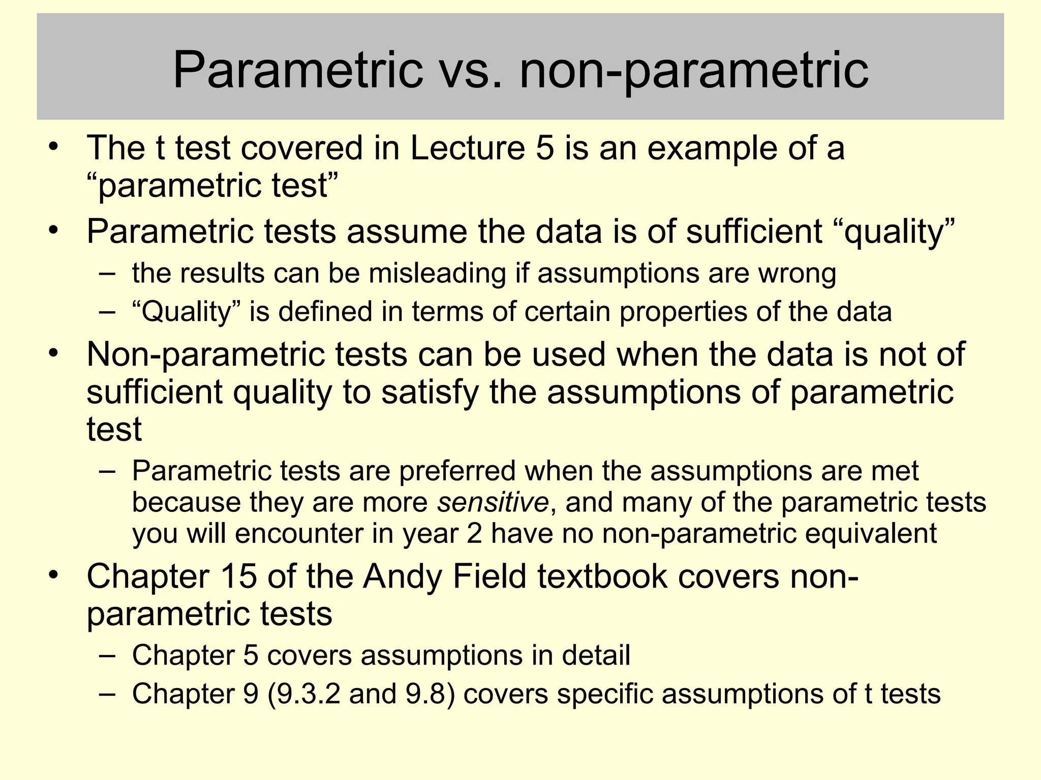
•The t test covered in Lecture 5 is an example of a
“parametric test”
• Parametric tests assume the data is of sufficient “quality”
– the results can be misleading if assumptions are wrong
– “Quality” is defined in terms of certain properties of the data
• Non-parametric tests can be used when the data is not of
sufficient quality to satisfy the assumptions of parametric
test
– Parametric tests are preferred when the assumptions are met
because they are more sensitive, and many of the parametric tests
you will encounter in year 2 have no non-parametric equivalent
• Chapter 15 of the Andy Field textbook covers non-
parametric tests
– Chapter 5 covers assumptions in detail
– Chapter 9 (9.3.2 and 9.8) covers specific assumptions of t tests
3.
Assumptions of ttests – a list
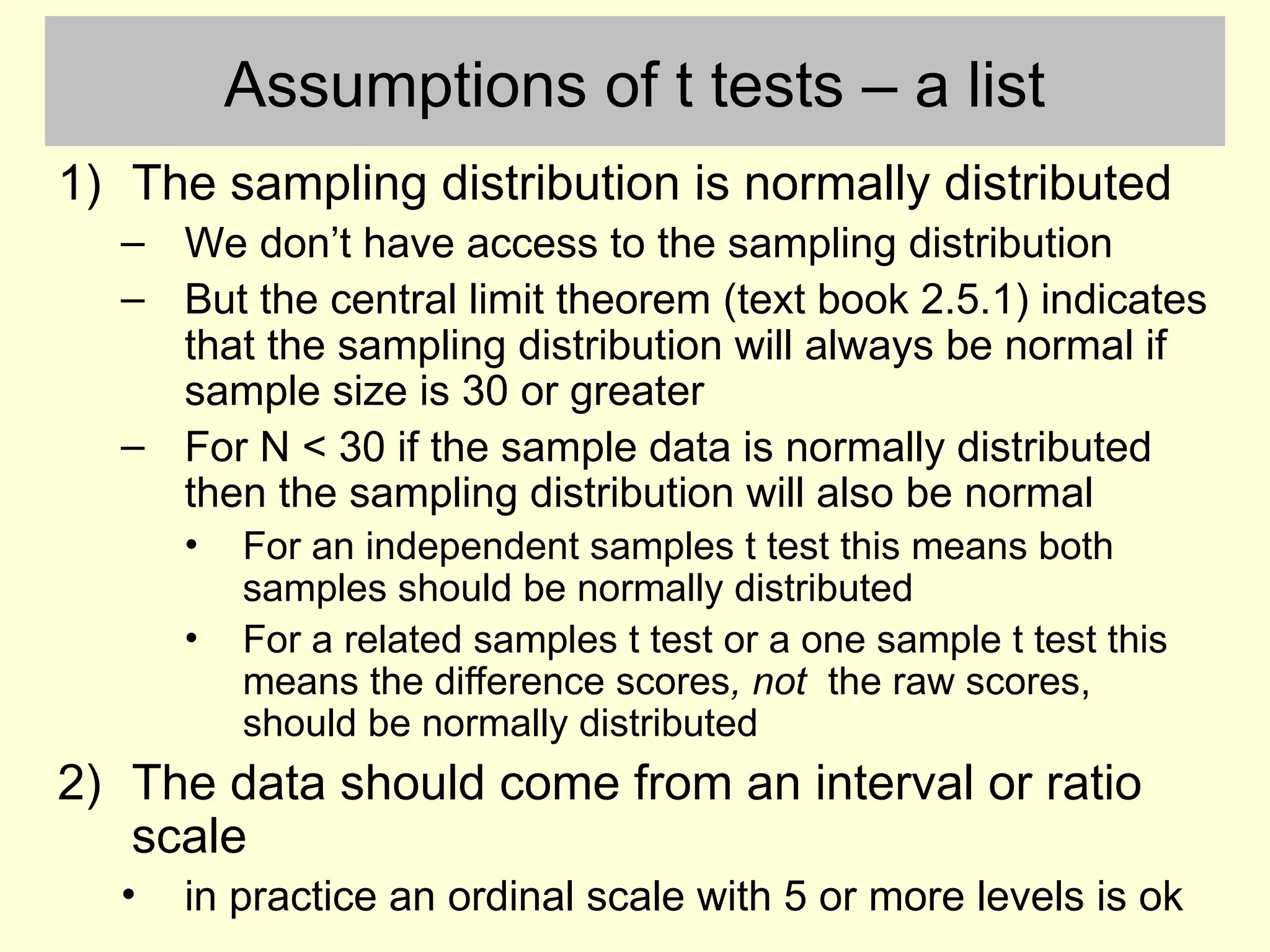
1) The sampling distribution is normally distributed
– We don’t have access to the sampling distribution
– But the central limit theorem (text book 2.5.1) indicates
that the sampling distribution will always be normal if
sample size is 30 or greater
– For N < 30 if the sample data is normally distributed
then the sampling distribution will also be normal
• For an independent samples t test this means both
samples should be normally distributed
• For a related samples t test or a one sample t test this
means the difference scores, not the raw scores,
should be normally distributed
2) The data should come from an interval or ratio
scale
• in practice an ordinal scale with 5 or more levels is ok
4.
Assumptions of ttests – a list
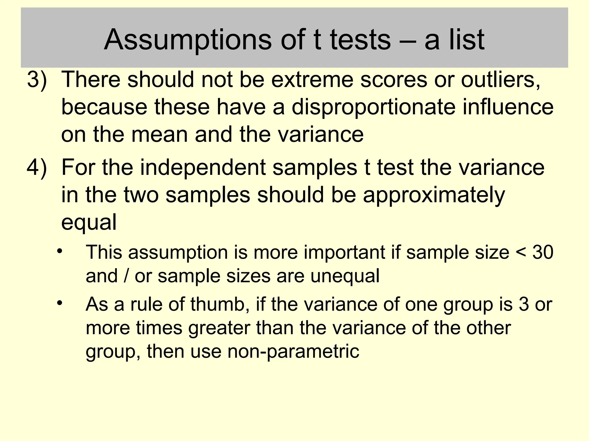
3) There should not be extreme scores or outliers,
because these have a disproportionate influence
on the mean and the variance
4) For the independent samples t test the variance
in the two samples should be approximately
equal
• This assumption is more important if sample size < 30
and / or sample sizes are unequal
• As a rule of thumb, if the variance of one group is 3 or
more times greater than the variance of the other
group, then use non-parametric
5.
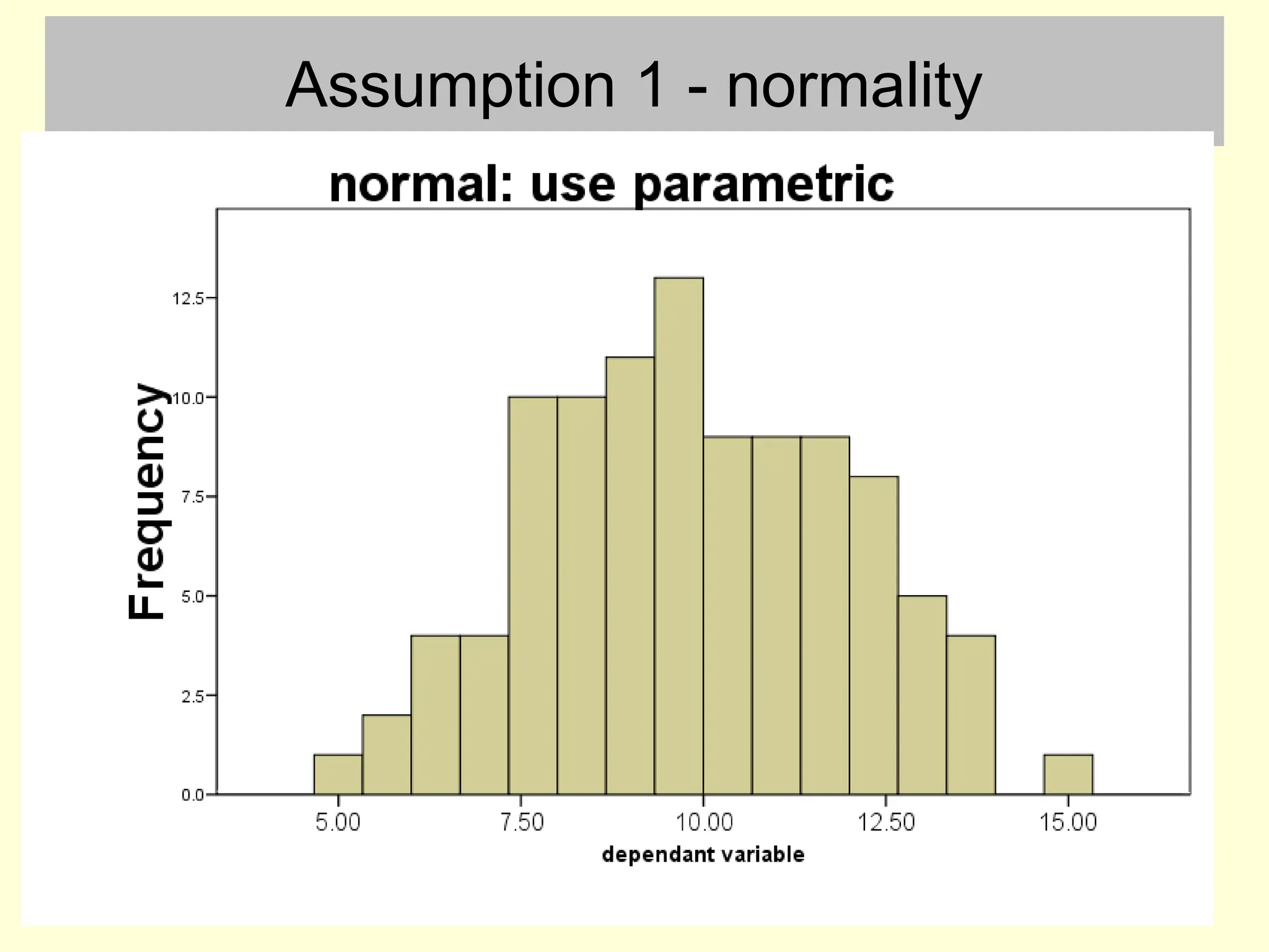
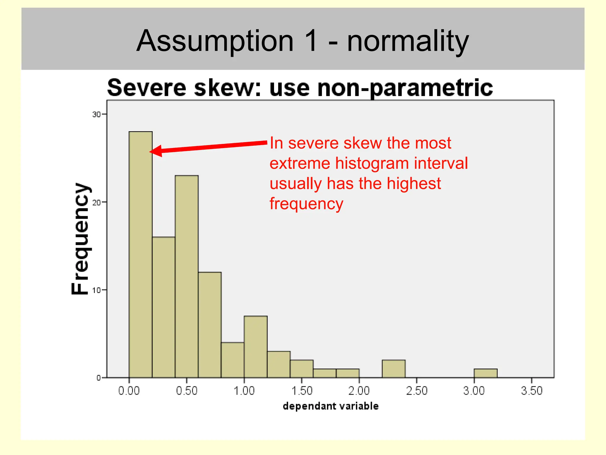
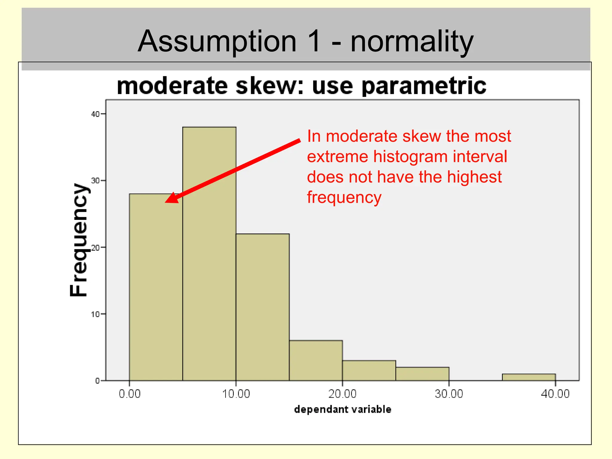
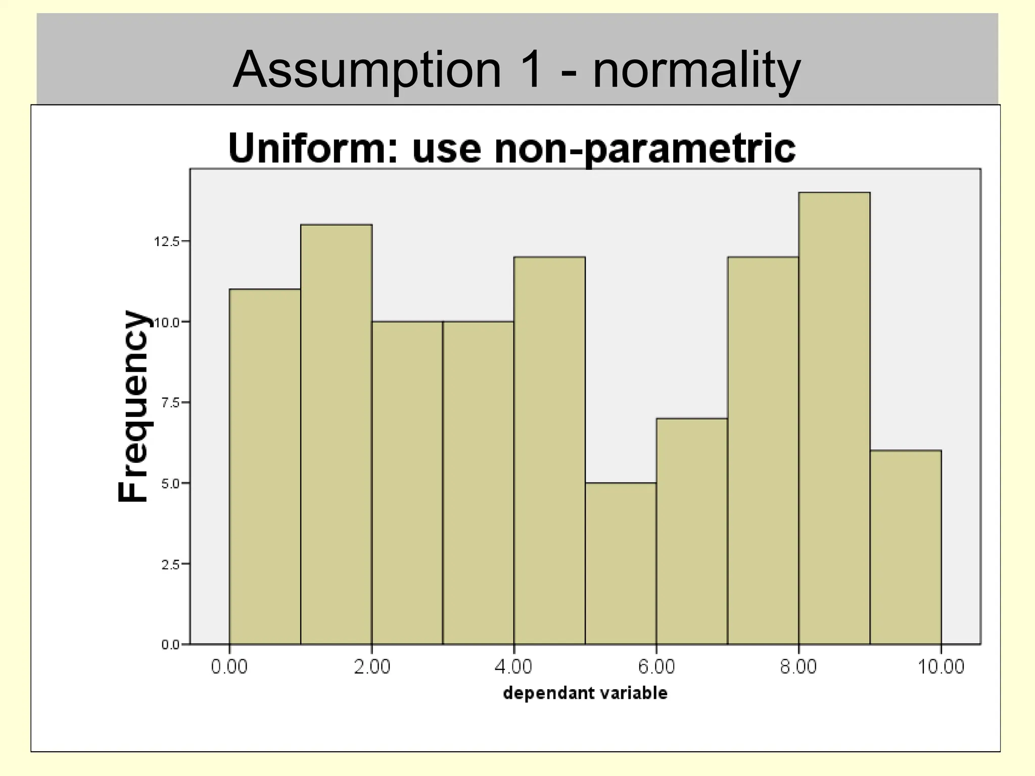
Assumption 1 -normality
• This can be checked by inspecting a histogram
– with small samples the histogram is unlikely to ever be
exactly bell shaped
• This assumption is only broken if there are large
and obvious departures from normality
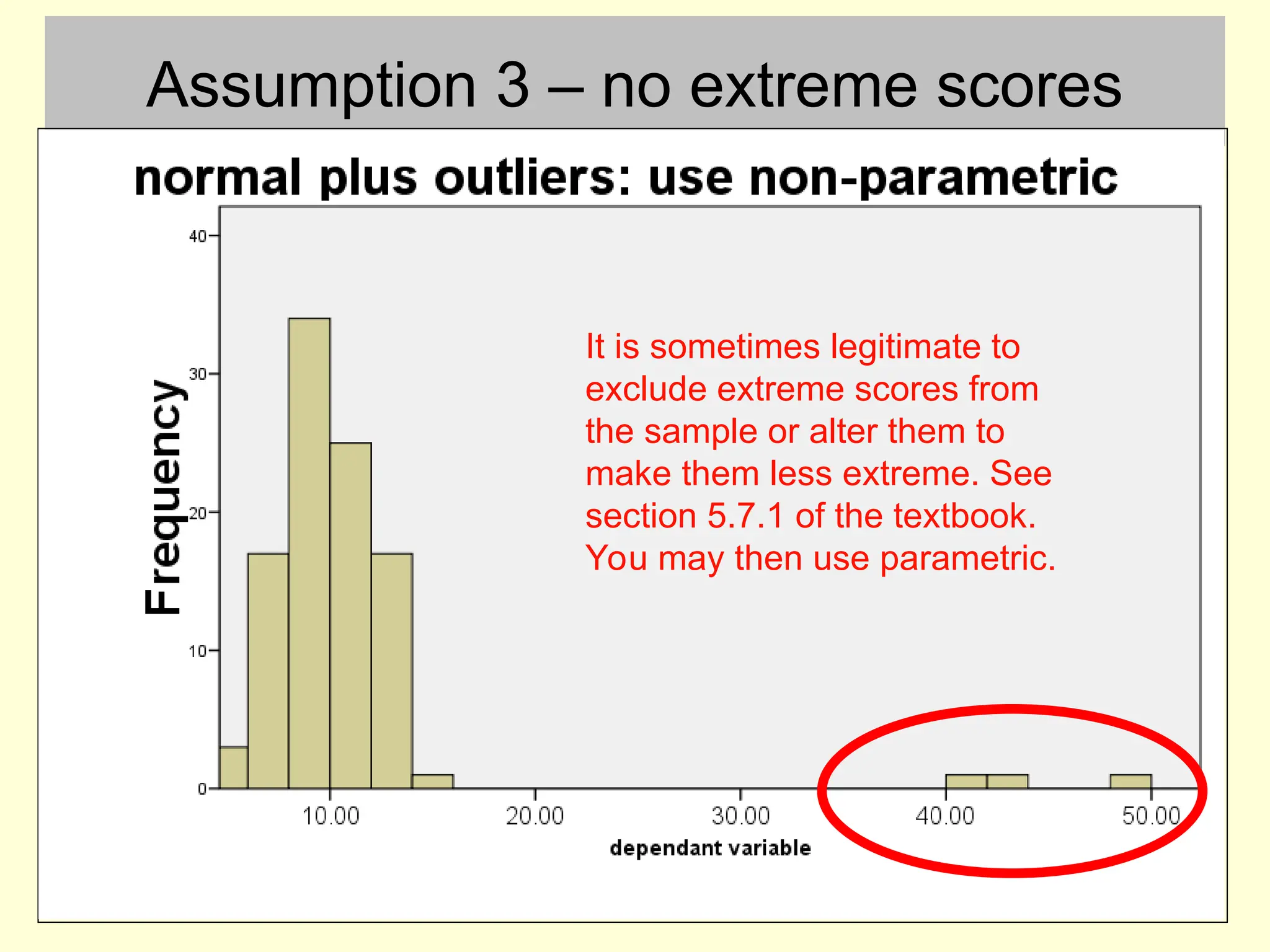
Assumption 3 –no extreme scores
It is sometimes legitimate to
exclude extreme scores from
the sample or alter them to
make them less extreme. See
section 5.7.1 of the textbook.
You may then use parametric.
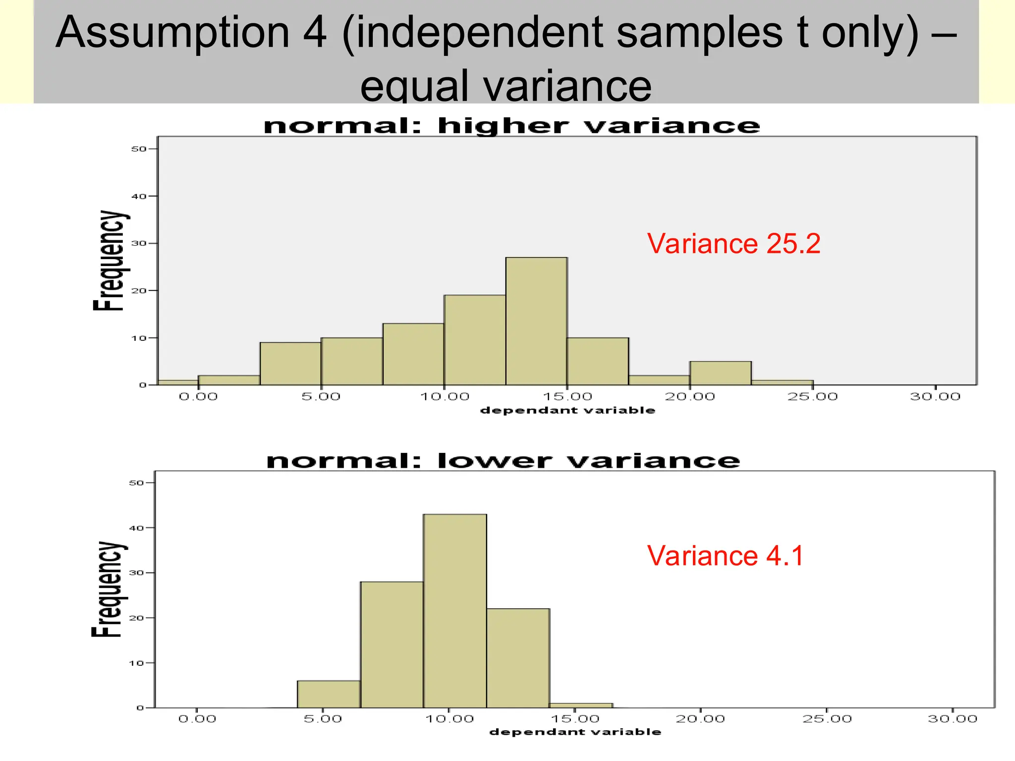
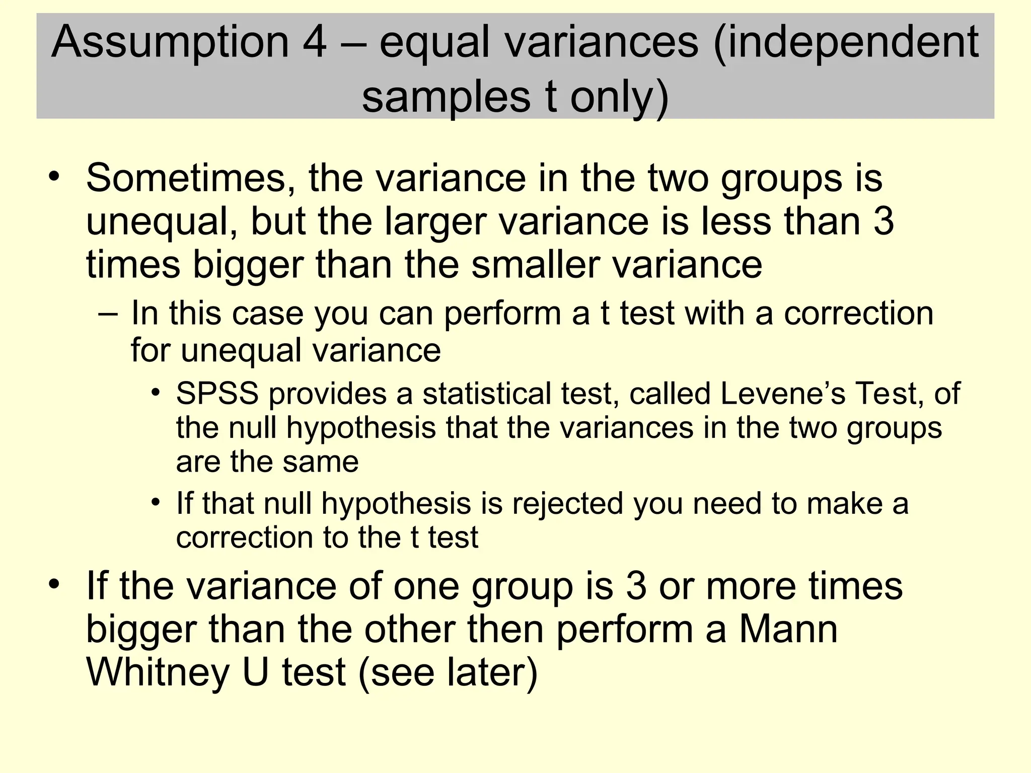
Assumption 4 –equal variances (independent
samples t only)
• Sometimes, the variance in the two groups is
unequal, but the larger variance is less than 3
times bigger than the smaller variance
– In this case you can perform a t test with a correction
for unequal variance
• SPSS provides a statistical test, called Levene’s Test, of
the null hypothesis that the variances in the two groups
are the same
• If that null hypothesis is rejected you need to make a
correction to the t test
• If the variance of one group is 3 or more times
bigger than the other then perform a Mann
Whitney U test (see later)
13.
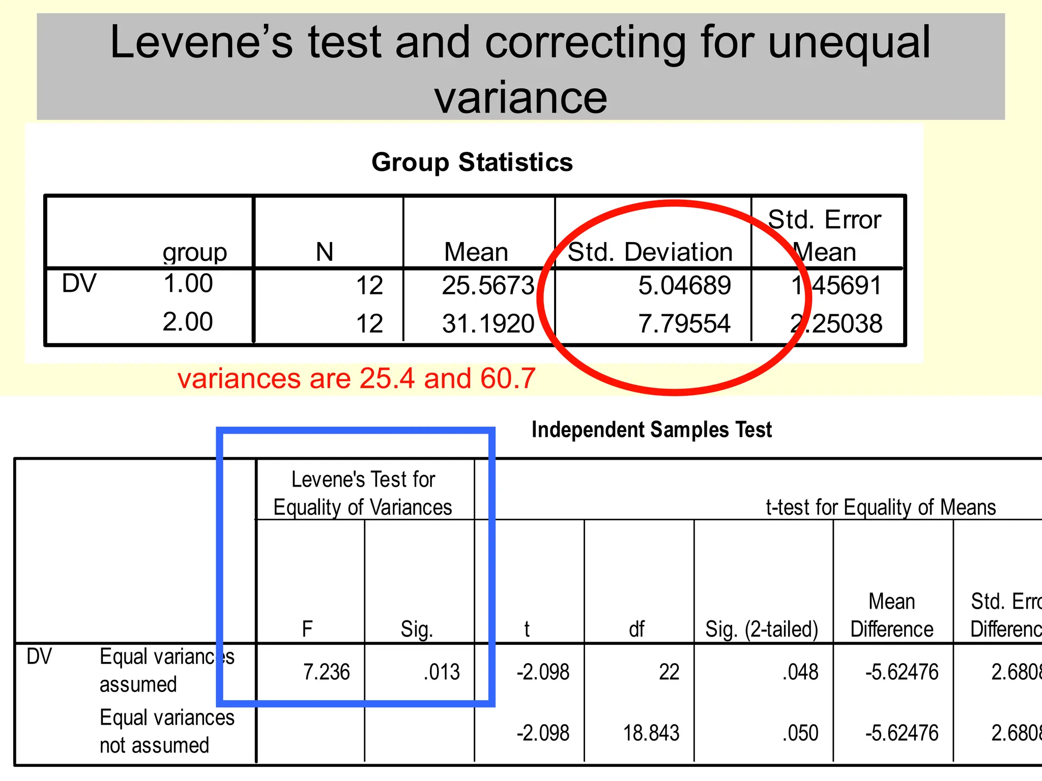
Levene’s test andcorrecting for unequal
variance
Group Statistics
12 25.5673 5.04689 1.45691
12 31.1920 7.79554 2.25038
group
1.00
2.00
DV
N Mean Std. Deviation
Std. Error
Mean
Independent Samples Test
7.236 .013 -2.098 22 .048 -5.62476 2.6808
-2.098 18.843 .050 -5.62476 2.6808
Equal variances
assumed
Equal variances
not assumed
DV
F Sig.
Levene's Test for
Equality of Variances
t df Sig. (2-tailed)
Mean
Difference
Std. Erro
Differenc
t-test for Equality of Means
variances are 25.4 and 60.7
14.
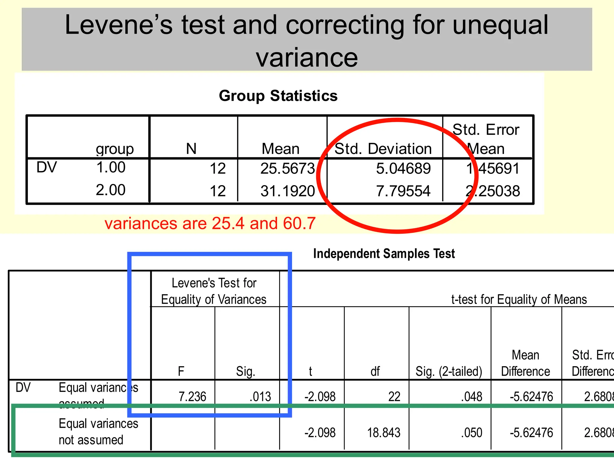
Levene’s test andcorrecting for unequal
variance
Group Statistics
12 25.5673 5.04689 1.45691
12 31.1920 7.79554 2.25038
group
1.00
2.00
DV
N Mean Std. Deviation
Std. Error
Mean
Independent Samples Test
7.236 .013 -2.098 22 .048 -5.62476 2.6808
-2.098 18.843 .050 -5.62476 2.6808
Equal variances
assumed
Equal variances
not assumed
DV
F Sig.
Levene's Test for
Equality of Variances
t df Sig. (2-tailed)
Mean
Difference
Std. Erro
Differenc
t-test for Equality of Means
variances are 25.4 and 60.7
15.
Digression: testing thenull hypothesis that
two samples have the same variance
• Suppose some researchers predict that children educated
in a traditional way will have a greater range of scores in
end of year tests compared to the modern approach
• 40 children are randomly allocated to either traditional or
modern classrooms
• The Levene’s Test can be used to test the null hypothesis
that the two groups show the same amount of dispersion
around the mean
16.
Non-parametric tests
• Theseare sometimes referred to as “distribution free”
tests, because they do not make assumptions about the
normality or variance of the data
• The Mann Whitney U test is appropriate for a 2 condition
independent samples design
• The Wilcoxon Signed Rank test is appropriate for a 2
condition related samples design
• If you have decided to use a non-parametric test then the
most appropriate measure of central tendency will
probably be the median
17.
Mann-Whitney U test
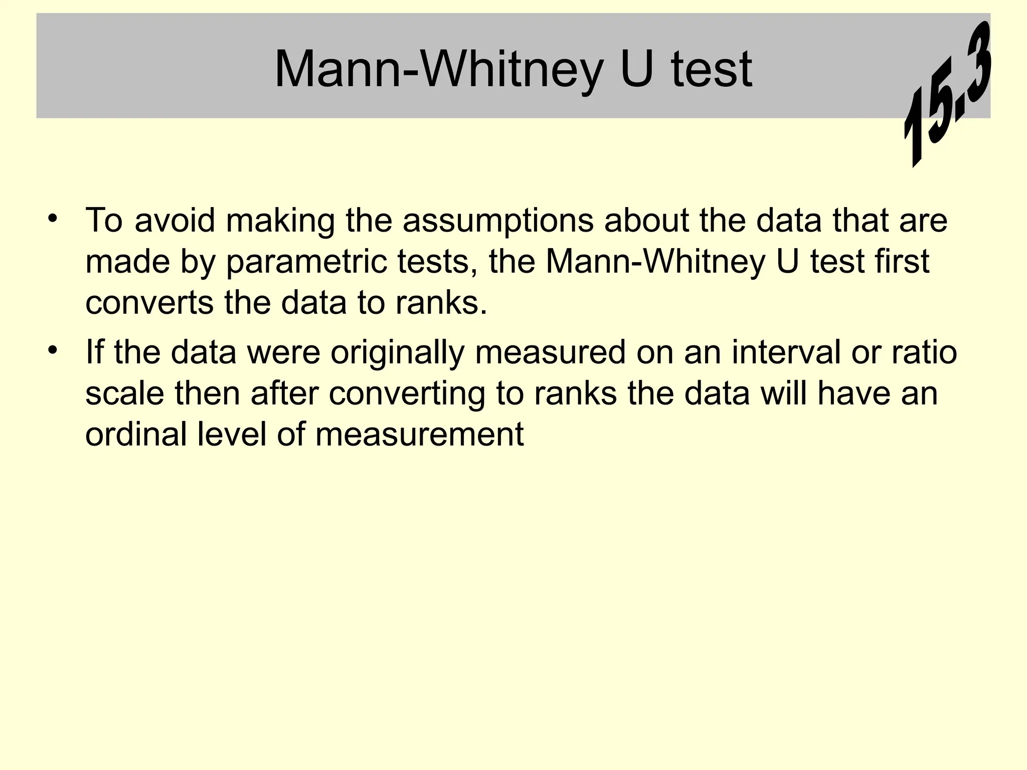
•To avoid making the assumptions about the data that are
made by parametric tests, the Mann-Whitney U test first
converts the data to ranks.
• If the data were originally measured on an interval or ratio
scale then after converting to ranks the data will have an
ordinal level of measurement
Mann-Whitney U test:ranking the data
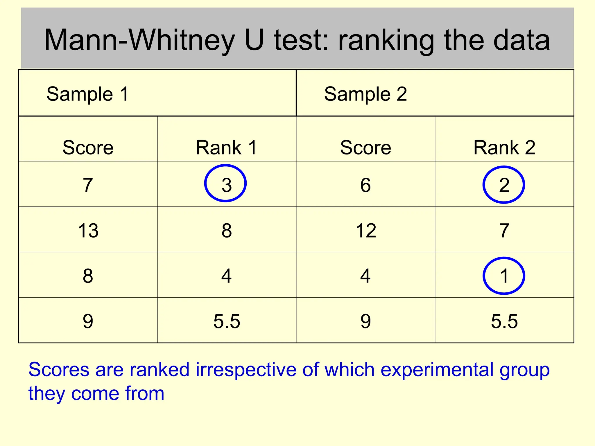
Sample 1 Sample 2
Score Rank 1 Score Rank 2
7 3 6 2
13 8 12 7
8 4 4 1
9 5.5 9 5.5
Scores are ranked irrespective of which experimental group
they come from
20.
Mann-Whitney U test:ranking the data
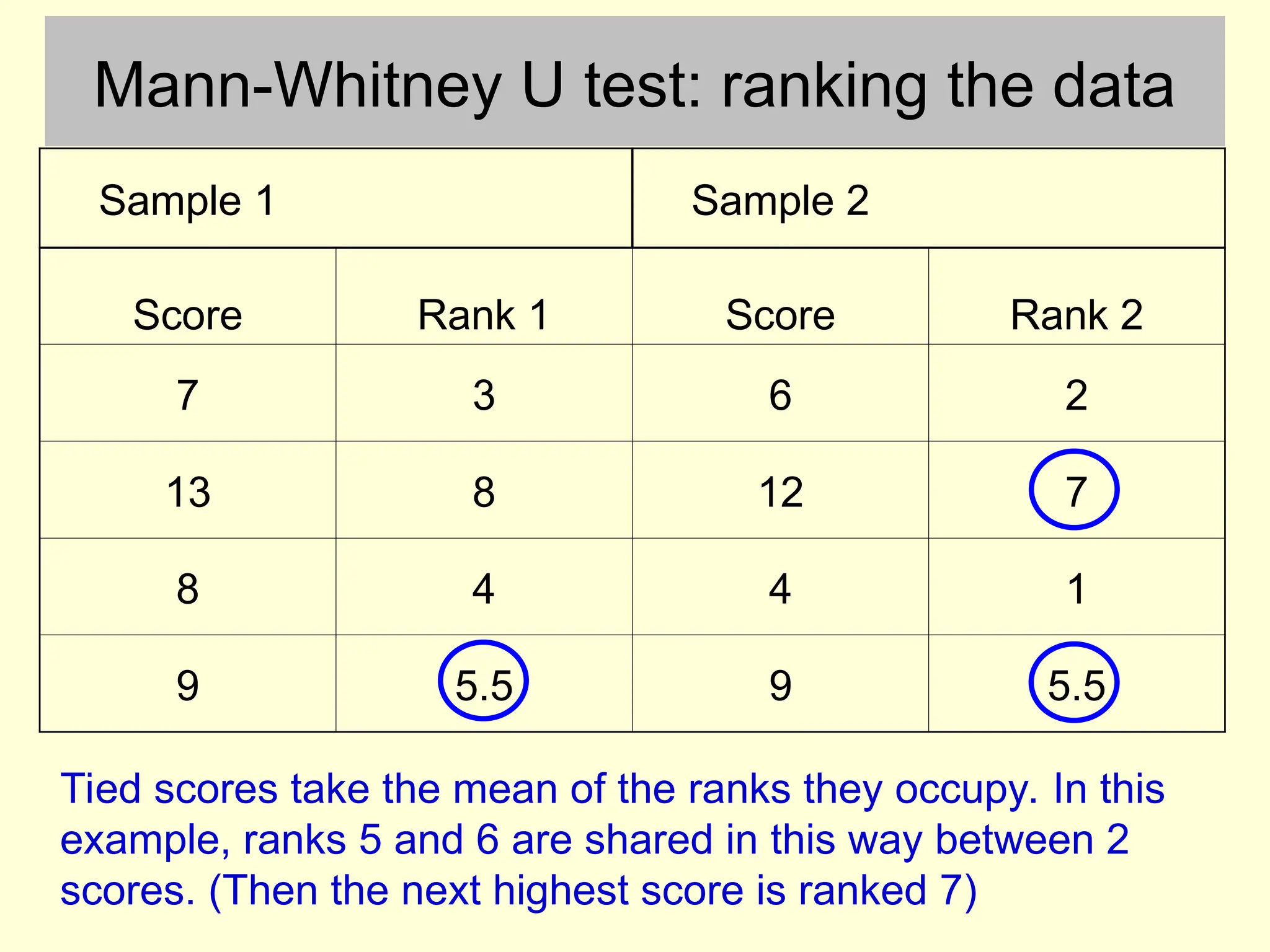
Sample 1 Sample 2
Score Rank 1 Score Rank 2
7 3 6 2
13 8 12 7
8 4 4 1
9 5.5 9 5.5
Tied scores take the mean of the ranks they occupy. In this
example, ranks 5 and 6 are shared in this way between 2
scores. (Then the next highest score is ranked 7)
21.
Rationale of Mann-WhitneyU
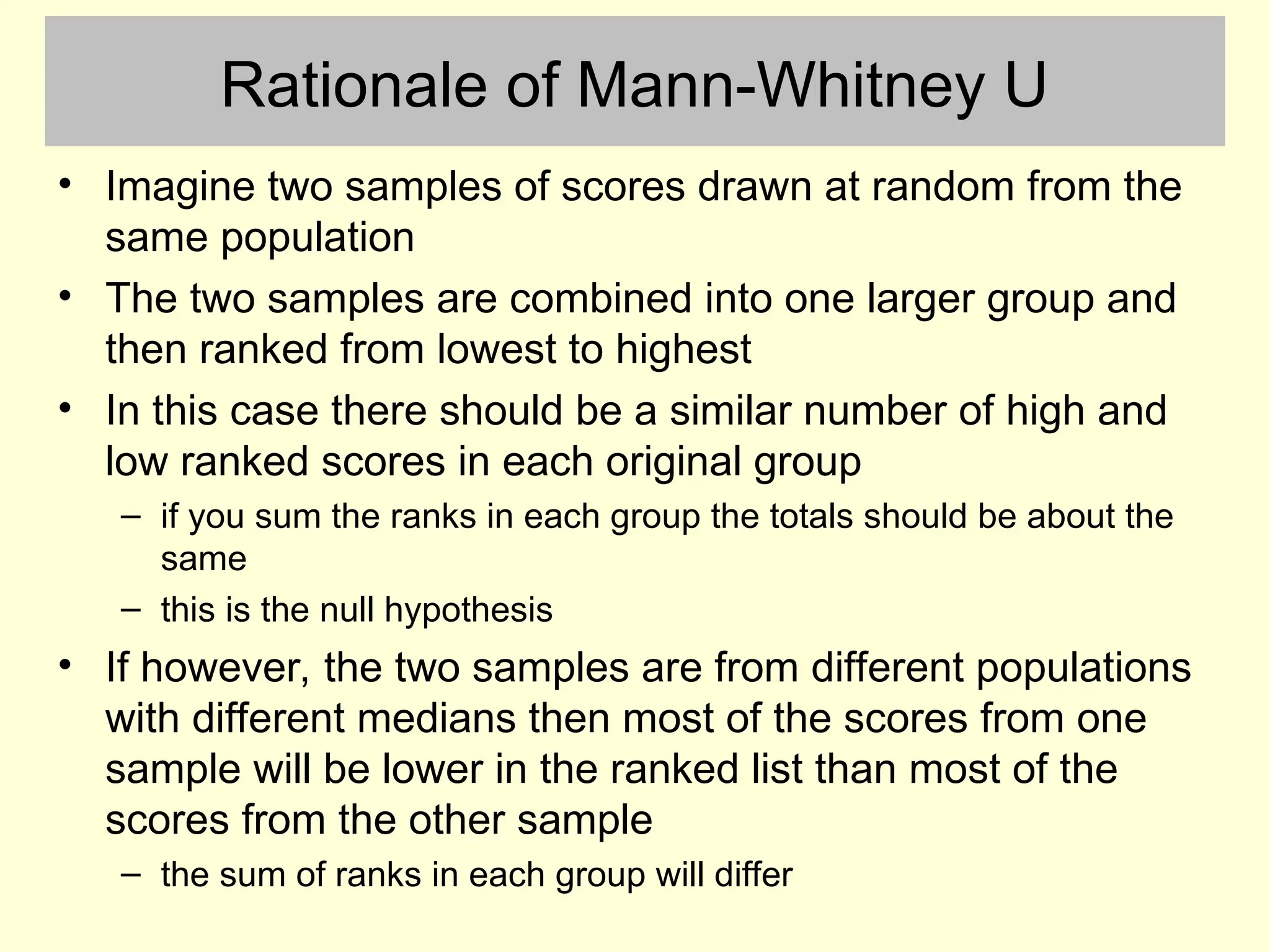
• Imagine two samples of scores drawn at random from the
same population
• The two samples are combined into one larger group and
then ranked from lowest to highest
• In this case there should be a similar number of high and
low ranked scores in each original group
– if you sum the ranks in each group the totals should be about the
same
– this is the null hypothesis
• If however, the two samples are from different populations
with different medians then most of the scores from one
sample will be lower in the ranked list than most of the
scores from the other sample
– the sum of ranks in each group will differ
22.
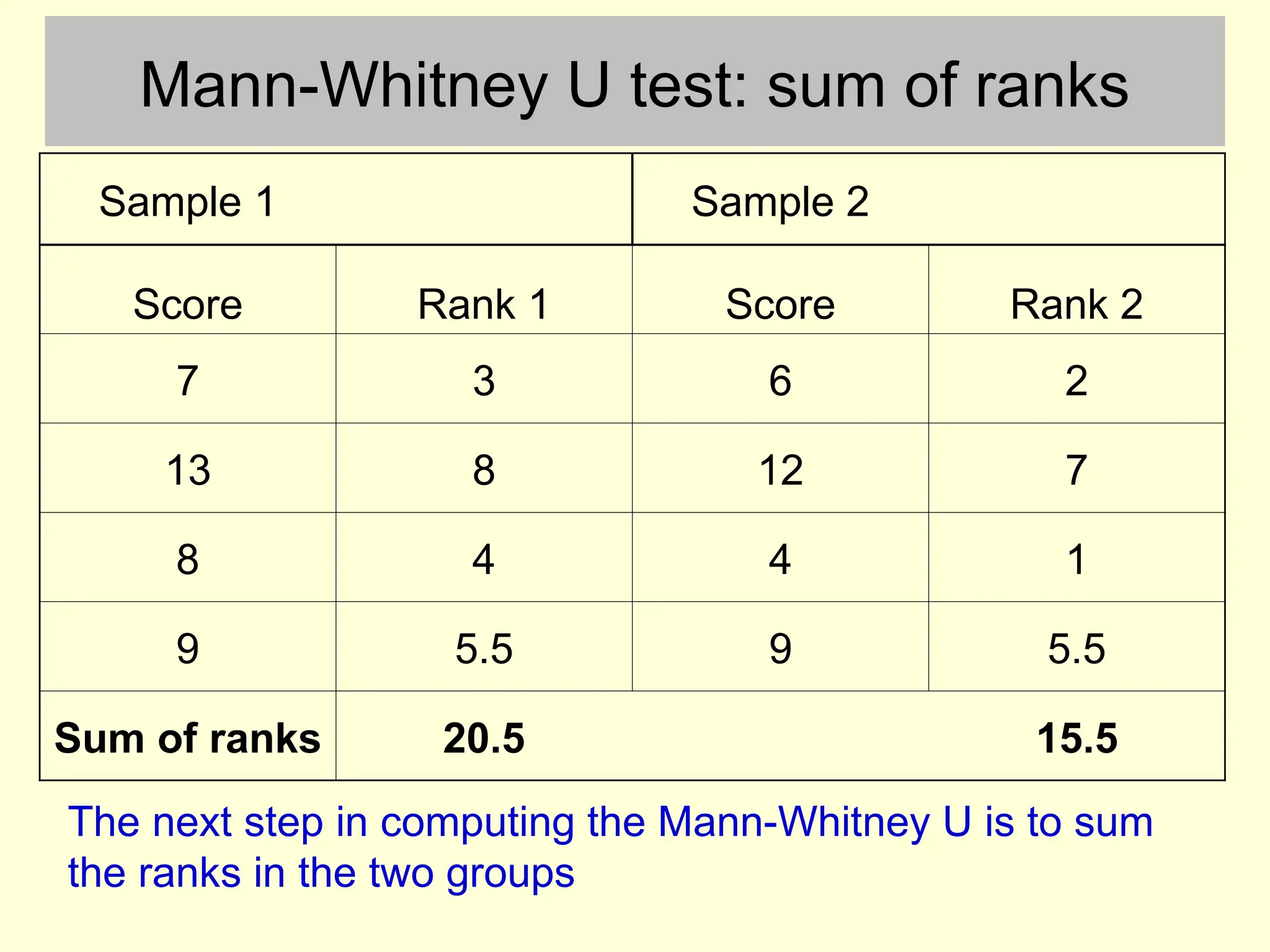
Mann-Whitney U test:sum of ranks
Sample 1 Sample 2
Score Rank 1 Score Rank 2
7 3 6 2
13 8 12 7
8 4 4 1
9 5.5 9 5.5
Sum of ranks 20.5 15.5
The next step in computing the Mann-Whitney U is to sum
the ranks in the two groups
23.
Mann Whitney U- SPSS
Ranks
12 10.75 129.00
12 14.25 171.00
24
group
1.00
2.00
Total
DV
N Mean Rank Sum of Ranks
Test Statisticsb
51.000
129.000
-1.212
.225
.242
a
Mann-Whitney U
Wilcoxon W
Z
Asymp. Sig. (2-tailed)
Exact Sig. [2*(1-tailed
Sig.)]
DV
Not corrected for ties.
a.
Grouping Variable: group
b.
The value of U is calculated
using a formula that compares
the summed ranks of the two
groups and takes into account
sample size
You don’t need to know the
formula
24.
Mann Whitney U- SPSS
Ranks
12 10.75 129.00
12 14.25 171.00
24
group
1.00
2.00
Total
DV
N Mean Rank Sum of Ranks
Test Statisticsb
51.000
129.000
-1.212
.225
.242
a
Mann-Whitney U
Wilcoxon W
Z
Asymp. Sig. (2-tailed)
Exact Sig. [2*(1-tailed
Sig.)]
DV
Not corrected for ties.
a.
Grouping Variable: group
b.
You should generally report the
asymptotic p value
To calculate this SPSS
converts the value of U to a Z
score, i.e. a value on the
standard normal distribution
The Z score is converted to a p
value in the same way as for
the Z test (lecture 4)
26.
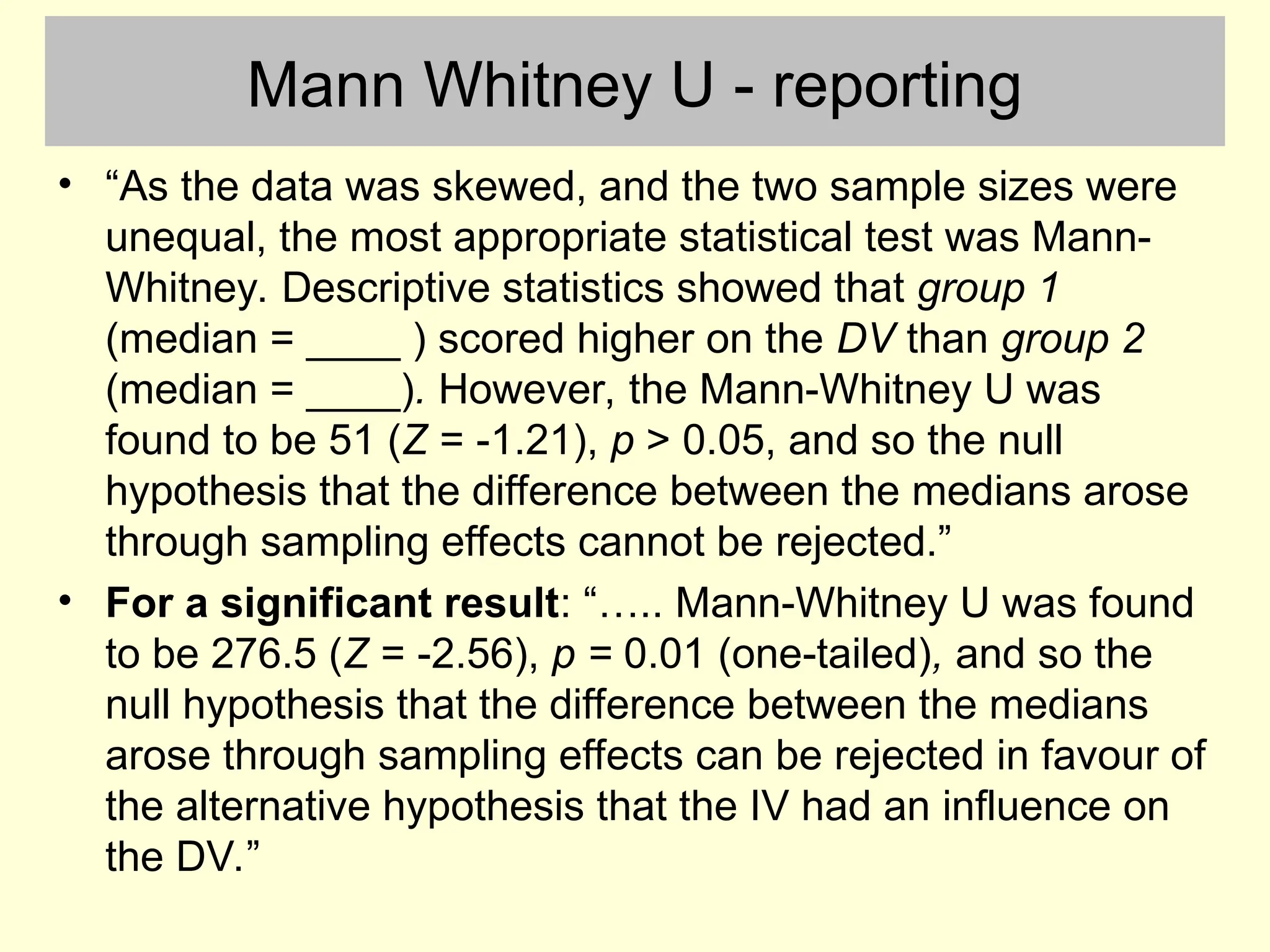
Mann Whitney U- reporting
• “As the data was skewed, and the two sample sizes were
unequal, the most appropriate statistical test was Mann-
Whitney. Descriptive statistics showed that group 1
(median = ____ ) scored higher on the DV than group 2
(median = ____). However, the Mann-Whitney U was
found to be 51 (Z = -1.21), p > 0.05, and so the null
hypothesis that the difference between the medians arose
through sampling effects cannot be rejected.”
• For a significant result: “….. Mann-Whitney U was found
to be 276.5 (Z = -2.56), p = 0.01 (one-tailed), and so the
null hypothesis that the difference between the medians
arose through sampling effects can be rejected in favour of
the alternative hypothesis that the IV had an influence on
the DV.”
27.
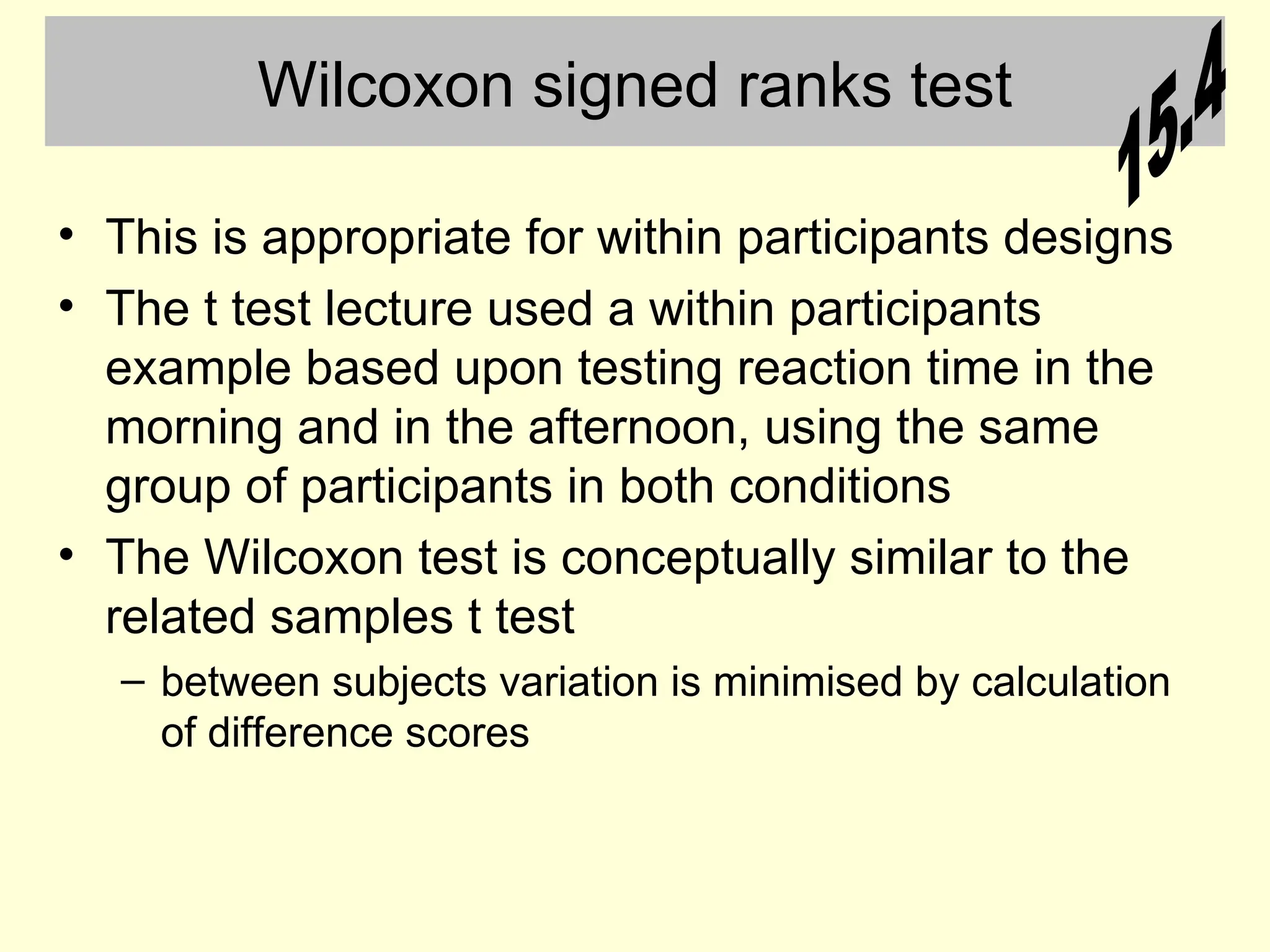
Wilcoxon signed rankstest
• This is appropriate for within participants designs
• The t test lecture used a within participants
example based upon testing reaction time in the
morning and in the afternoon, using the same
group of participants in both conditions
• The Wilcoxon test is conceptually similar to the
related samples t test
– between subjects variation is minimised by calculation
of difference scores
28.
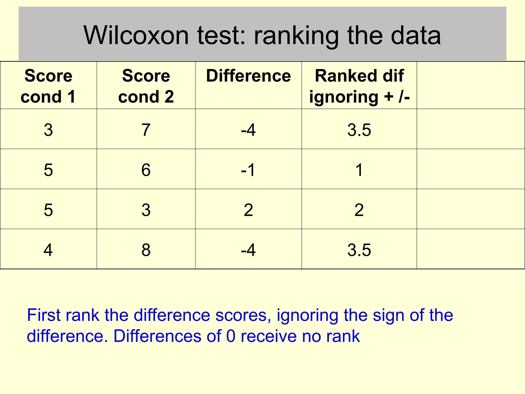
Wilcoxon test: rankingthe data
Score
cond 1
Score
cond 2
Difference Ranked dif
ignoring + /-
3 7 -4 3.5
5 6 -1 1
5 3 2 2
4 8 -4 3.5
First rank the difference scores, ignoring the sign of the
difference. Differences of 0 receive no rank
29.
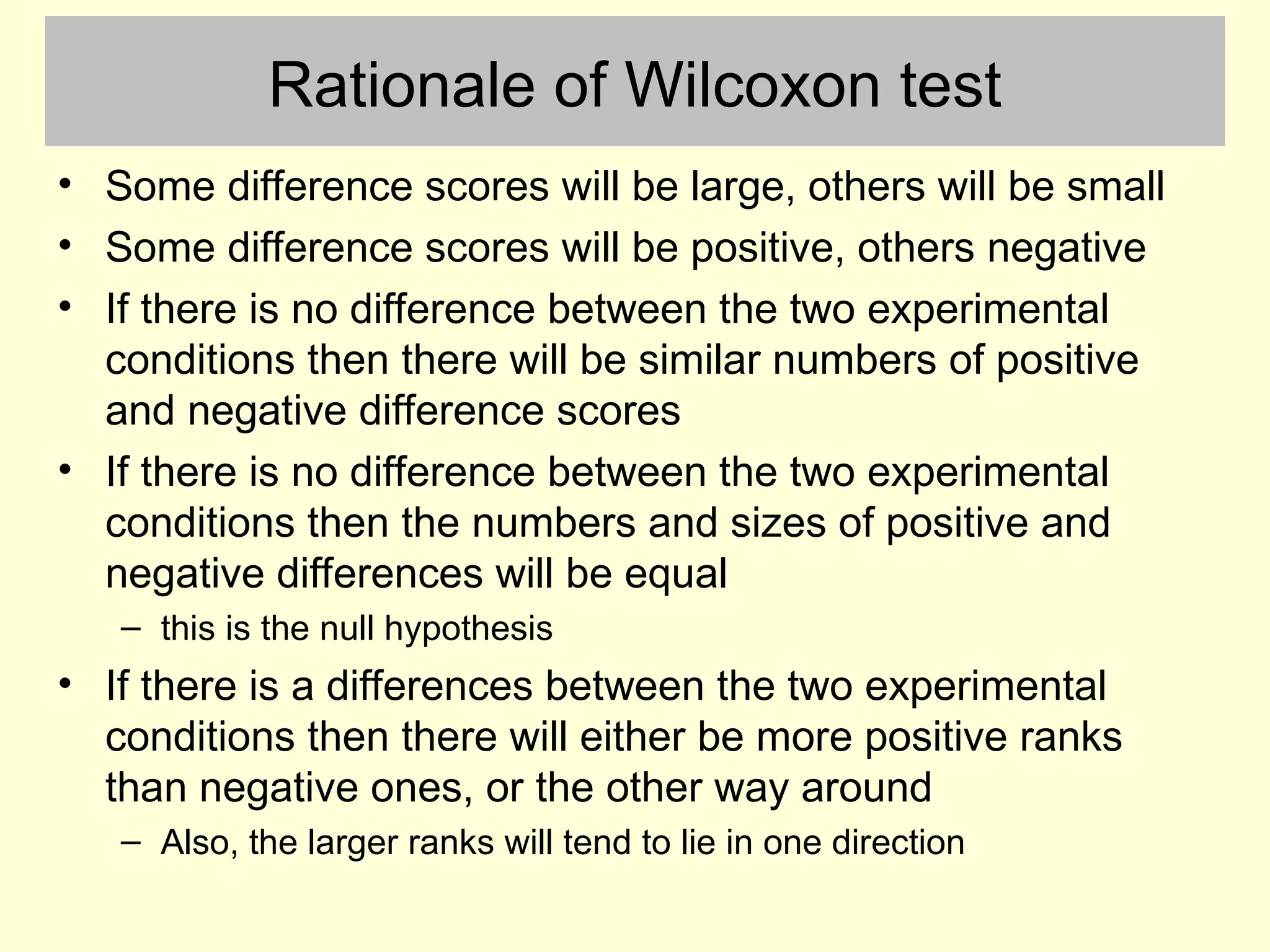
Rationale of Wilcoxontest
• Some difference scores will be large, others will be small
• Some difference scores will be positive, others negative
• If there is no difference between the two experimental
conditions then there will be similar numbers of positive
and negative difference scores
• If there is no difference between the two experimental
conditions then the numbers and sizes of positive and
negative differences will be equal
– this is the null hypothesis
• If there is a differences between the two experimental
conditions then there will either be more positive ranks
than negative ones, or the other way around
– Also, the larger ranks will tend to lie in one direction
30.
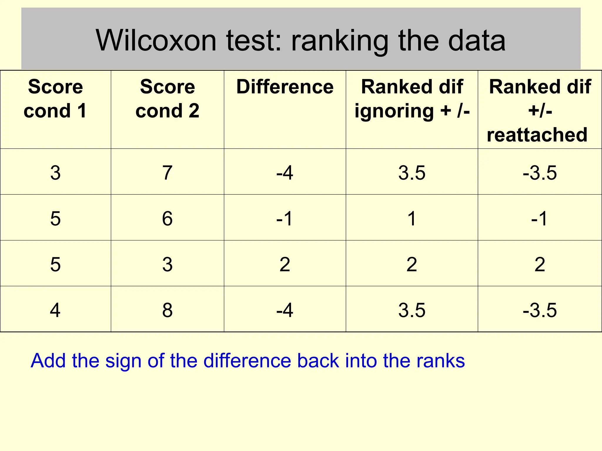
Wilcoxon test: rankingthe data
Score
cond 1
Score
cond 2
Difference Ranked dif
ignoring + /-
Ranked dif
+/-
reattached
3 7 -4 3.5 -3.5
5 6 -1 1 -1
5 3 2 2 2
4 8 -4 3.5 -3.5
Add the sign of the difference back into the ranks
31.
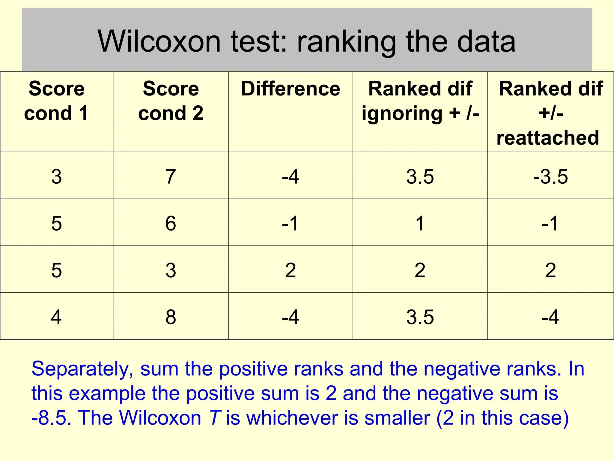
Wilcoxon test: rankingthe data
Score
cond 1
Score
cond 2
Difference Ranked dif
ignoring + /-
Ranked dif
+/-
reattached
3 7 -4 3.5 -3.5
5 6 -1 1 -1
5 3 2 2 2
4 8 -4 3.5 -4
Separately, sum the positive ranks and the negative ranks. In
this example the positive sum is 2 and the negative sum is
-8.5. The Wilcoxon T is whichever is smaller (2 in this case)
32.
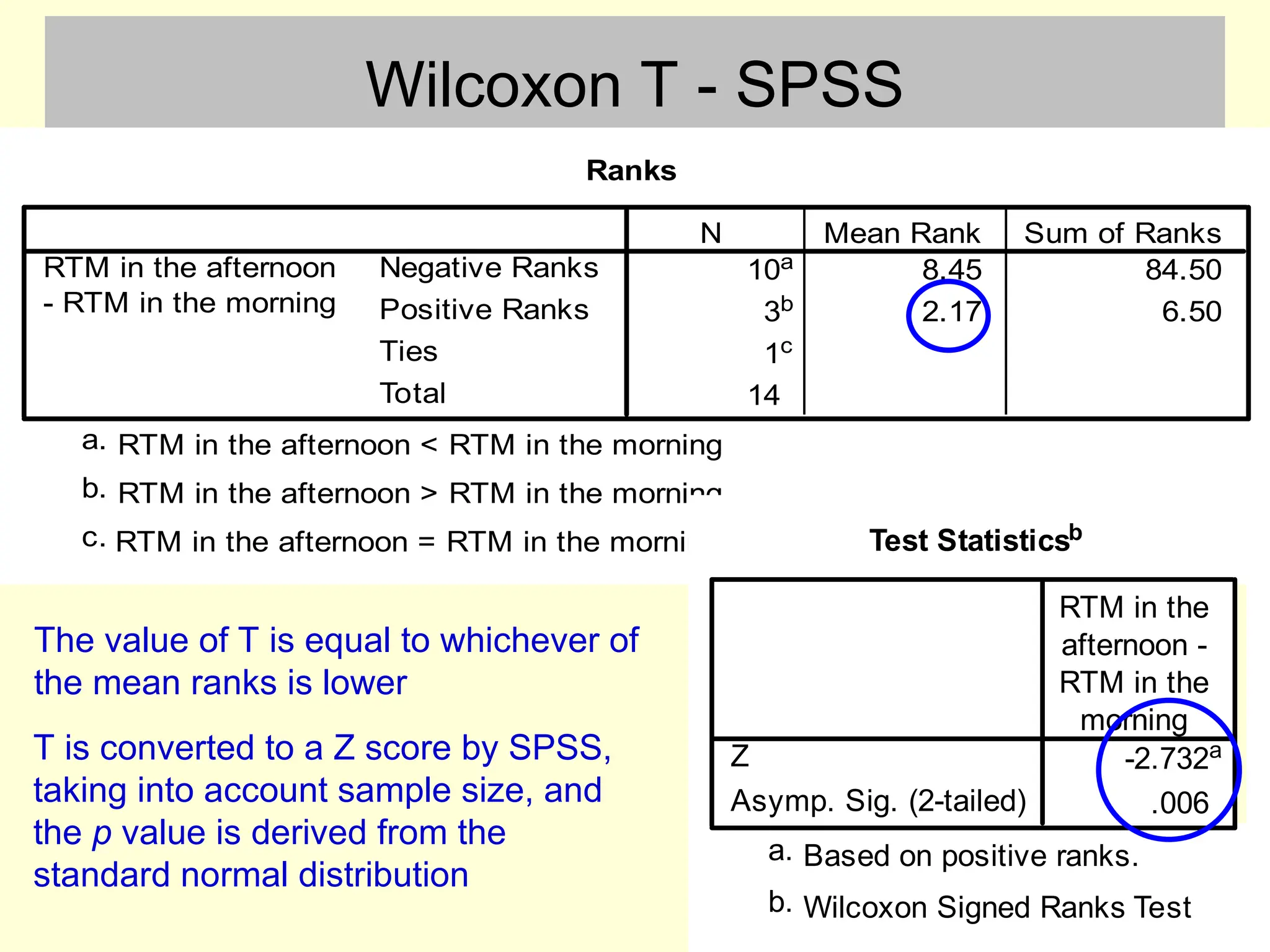
Wilcoxon T -SPSS
Ranks
10a 8.45 84.50
3b 2.17 6.50
1c
14
Negative Ranks
Positive Ranks
Ties
Total
RTM in the afternoon
- RTM in the morning
N Mean Rank Sum of Ranks
RTM in the afternoon < RTM in the morning
a.
RTM in the afternoon > RTM in the morning
b.
RTM in the afternoon = RTM in the morning
c. Test Statisticsb
-2.732a
.006
Z
Asymp. Sig. (2-tailed)
RTM in the
afternoon -
RTM in the
morning
Based on positive ranks.
a.
Wilcoxon Signed Ranks Test
b.
The value of T is equal to whichever of
the mean ranks is lower
T is converted to a Z score by SPSS,
taking into account sample size, and
the p value is derived from the
standard normal distribution
33.
Wilcoxon T -reporting
• “As the difference scores were not normally distributed,
the most appropriate statistical test was the Wilcoxon
signed-rank test. Descriptive statistics showed that
measurement in condition 1 (median = ____ ) produced
higher scores than in condition 2 (median = ____). The
Wilcoxon test (T = 2.17) was converted into a Z score of -
2.73, p = 0.006 (two tailed). It can therefore be concluded
that the experimental and control treatments produced
different scores.”
34.
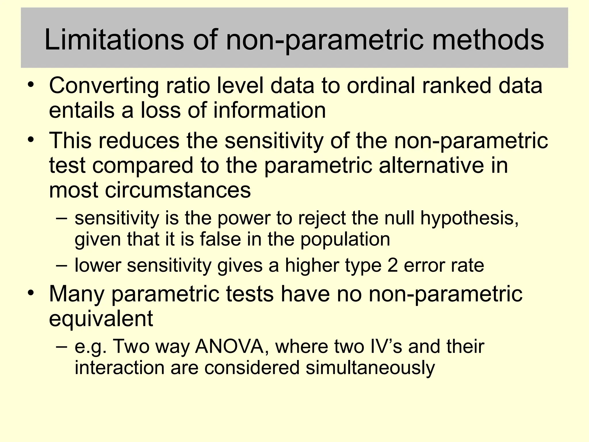
Limitations of non-parametricmethods
• Converting ratio level data to ordinal ranked data
entails a loss of information
• This reduces the sensitivity of the non-parametric
test compared to the parametric alternative in
most circumstances
– sensitivity is the power to reject the null hypothesis,
given that it is false in the population
– lower sensitivity gives a higher type 2 error rate
• Many parametric tests have no non-parametric
equivalent
– e.g. Two way ANOVA, where two IV’s and their
interaction are considered simultaneously
Editor's Notes
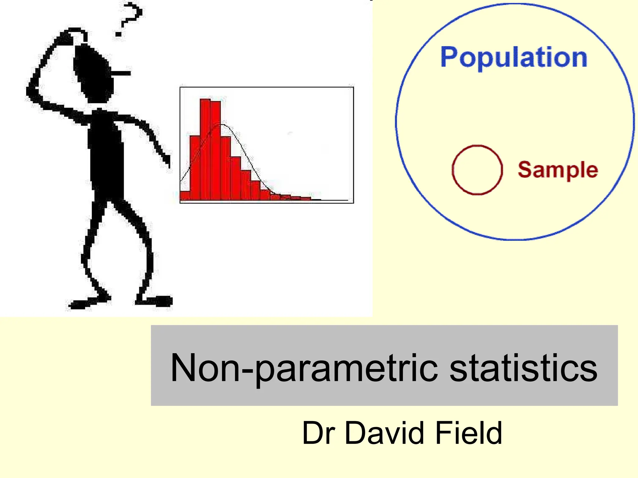
#1 Last weeks lecture was about t tests. At the time I did not tell you that t tests are a member of a family of statistical tests called parametric tests. They are called parametric tests because they use sample to make inferences about population parameters (the mean of a population is technically known as a parameter, whereas the mean of a sample is technically known as a statistic). Now, parametric tests are only appropriate when the data is of a good quality and certain assumptions are met. When those assumptions are not met we need to se a different set of tests from a family called non-parametric tests. Today’s lecture will seek to do two things – guide you through the process of learning how to decide between parametric and non-parametric tests, and then explain the rationale of the nonparametric tests and how to report them.
#2 The last bullet point explains why we don’t always use non-parametric tests.
Sensitivity refers to the tests ability to reject the null hypothesis for a sample, given that it is actually false in the population.
#3 The reason the sampling distribution needs to be normally distributed is because the t distribution that was shown visually in lecture 5 is built using 2 assumptions. The first assumption is that the null hypothesis is true, and the second assumption is the underlying population of scores that has been sampled from is normally distributed. If the underlying population of scores was quite skewed, and the null hypothesis was true, then the frequency histogram of a large number of small samples from the population would not look like a t distribution. In a sense, the t distribution is a model of the underlying sampling distribution.
#6 I want you to test the normality assumption by plotting histograms and making a visual judgment. There are more formal ways, but they all have problems anyway.
#9 A uniform distribution is one with no clear peak in the middle, or even to the left or right. Such as obtained by rolling a dice many times.
#10 Remember that extreme scores have a disproportionate influence on means and variance. If you find extreme scores you can use non-parametric. An alternative is to alter the extreme scores so that they are still the highest in the data, but only by a small amount rather than a huge amount. Another alternative is to exclude those data points and use a parametric test. To do that you have to make the case that those data points are from “another” population and were sampled by accident. this can include things like a participant who did not try to do the experiment properly.
#11 These two histograms illustrate a fairly extreme example of a common problem. The sample sizes are the same, and I have adjusted the histogram x and y axis values so that the two graphs are directly comparable. Both samples conform to a normal distribution. It is clear that the means are similar, but the variance / SD is very different. If you calculate descriptive statistics and the variance of one group is 3 times bigger than the other you need to use a non-parametric test. Otherwise, you can get away with a corrected version of the t test (see later)
#13 The SPSS output for the t test gives you the SD instead of variance (annoyingly) so you need to square the SD or get it from another SPSS operation, such as Explore, in order to check the *3 rule. In this case the *3 rule is not violated so we can use a t test.
When performing an independent samples t test, if the two sample SD’s are even slightly different you should first check if the Levene’s test for equality of variances is significant. If and only if it is non-significant (i.e. p > 0.05), then this fails to rejects the null hypothesis that the two sample variances are equal, allowing you treat them as equal. If Levene's test suggests that the variances are unequal you should then report the t test values from the bottom row “equal variances not assumed”. The value of t is sometimes different, and the df will be reduced, and will have decimal places. Just report the values from the bottom row instead of the top row.
#14 The SPSS output for the t test gives you the SD instead of variance (annoyingly) so you need to sqaure the SD or get it from another SPSS operation, such as Explore, in order to check the *3 rule. In this case the *3 rule is not violated so we can use a t test.
When performing an independent samples t test, if the two sample SD’s are even slightly different you should first check if the Levene’s test for equality of variances is significant. If and only if it is non-significant (i.e. p > 0.05), then this fails to rejects the null hypothesis that the two sample variances are equal, allowing you treat them as equal. If Levene's test suggests that the variances are unequal you should then report the t test values from the bottom row “equal variances not assumed”. The value of t is sometimes different, and the df will be reduced, and will have decimal places. Just report the values from the bottom row instead of the top row.
#16 Just as the related samples t test was able to make use of difference scores as a way of reducing the error term, so the wilcoxon will also be able to make use of difference scores in its ranking procedure. Difference scores may not be used in any independent samples procedure.
#22 In this example the summed ranks for one group is higher than the other, and this begins to suggest that the sorted and ranked scores are not arranged at random in the combined list of ranked scores, so maybe the null hypothesis is going to be rejected in this case.
The summed ranks are converted to the U statistic using a formula that takes into account the sample size.
#23 The summed ranks are converted to the U statistic using a formula that takes into account the sample size (you don’t need to know the details of this). In order to convert U to a p value, SPSS first converts U to a value on the standard normal distribution, i.e. a Z score.
#24 The summed ranks are converted to the U statistic using a formula that takes into account the sample size (you don’t need to know the details of this). In order to convert U to a p value, SPSS first converts U to a value on the standard normal distribution, i.e. a Z score.
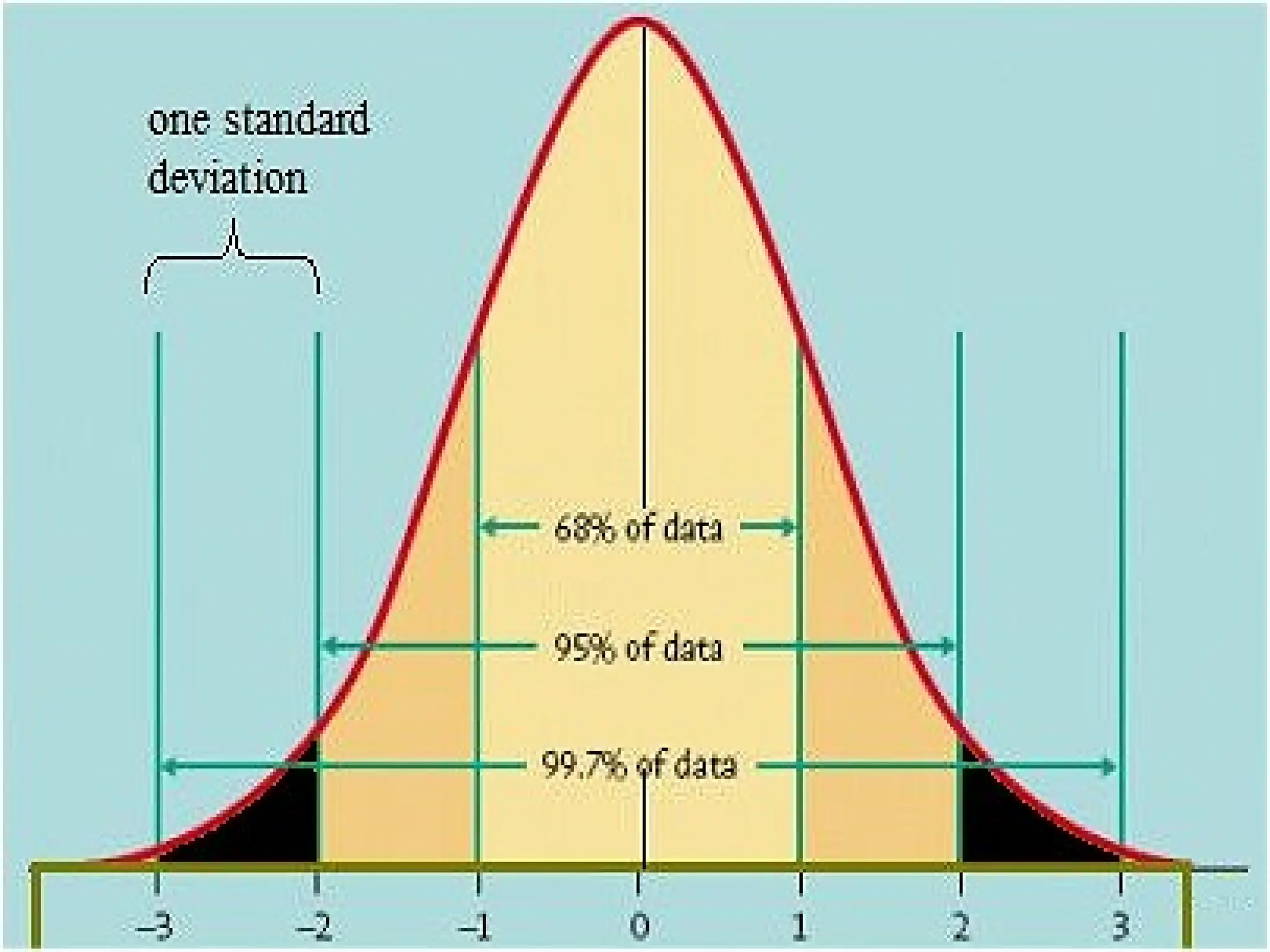
#25 Here is a standard normal distribution, and the x axis in units of SD is the same as the z statistic. The values z must exceed for a two tailed 0.05 p value are colored in black. In the mann whitney example on the preceding slide, you can see that the z o -1.22 is not sufficiently extreme to pass 0.05. If you drew a single case at random from the z distribution it would be 22% likely to have an unsigned value of greater than 1.22.
#26 Notice that SPSS converts the value of U to a z score, which is a value on the standard normal distribution (SND). The P value it reports is just the probability of a z score of that magnitude being picked by random sampling of a single score from the SND. You should recall that z score 1.95 = 0.05, z score 2.5 = 0.01 and z score 3 = 0.001 in terms of probability.
Note that if the hypothesis was two tailed you’d need to indicate that instead of one-tailed in the significant version of reporting a result.
#31 There is an imbalance in the sum of the ranks for this very small data set, suggesting that the null hypothesis might be rejected
#33 Note that you still have to deal with the one tailed versus two tailed thing with Wilcoxon. SPSS gives 2 tailed probability.
#34 Converting the times that runners take to complete a marathon into finishing positions caused you to loose the information that tells you whether the race was close or had a clear winner
ANOVA will be covered next year. In ANOVA you might have an experiment with 4 conditions, made up of a 2 by 2 grid of two IV’s each of which has two levels. For example, we might measure reaction time in the morning and the afternoon, and we might also test the effect of caffeine versus no caffeine. This results in four groups (caffeine morning, caffeine afternoon, no-caffeine morning, and no-caffeine afternoon). Such a design allows you to assess the “interaction”, i.e. whether the effects of caffeine on rtm are different in the morning compared to the effect of caffeinge on rtm in the afternoon. (Unfortunately, there is no non-parametric method for assessing the “interaction”)

![Mann Whitney U - SPSS
Ranks
12 10.75 129.00
12 14.25 171.00
24
group
1.00
2.00
Total
DV
N Mean Rank Sum of Ranks
Test Statisticsb
51.000
129.000
-1.212
.225
.242
a
Mann-Whitney U
Wilcoxon W
Z
Asymp. Sig. (2-tailed)
Exact Sig. [2*(1-tailed
Sig.)]
DV
Not corrected for ties.
a.
Grouping Variable: group
b.
The value of U is calculated
using a formula that compares
the summed ranks of the two
groups and takes into account
sample size
You don’t need to know the
formula](https://image.slidesharecdn.com/py1pr1statslecture6-250716062718-dcaed352/75/PY1PR1_stats_lecture_6-with-electronics-ppt-23-2048.jpg)
![Mann Whitney U - SPSS
Ranks
12 10.75 129.00
12 14.25 171.00
24
group
1.00
2.00
Total
DV
N Mean Rank Sum of Ranks
Test Statisticsb
51.000
129.000
-1.212
.225
.242
a
Mann-Whitney U
Wilcoxon W
Z
Asymp. Sig. (2-tailed)
Exact Sig. [2*(1-tailed
Sig.)]
DV
Not corrected for ties.
a.
Grouping Variable: group
b.
You should generally report the
asymptotic p value
To calculate this SPSS
converts the value of U to a Z
score, i.e. a value on the
standard normal distribution
The Z score is converted to a p
value in the same way as for
the Z test (lecture 4)](https://image.slidesharecdn.com/py1pr1statslecture6-250716062718-dcaed352/75/PY1PR1_stats_lecture_6-with-electronics-ppt-24-2048.jpg)


![Mann Whitney U - SPSS
Ranks
12 10.75 129.00
12 14.25 171.00
24
group
1.00
2.00
Total
DV
N Mean Rank Sum of Ranks
Test Statisticsb
51.000
129.000
-1.212
.225
.242
a
Mann-Whitney U
Wilcoxon W
Z
Asymp. Sig. (2-tailed)
Exact Sig. [2*(1-tailed
Sig.)]
DV
Not corrected for ties.
a.
Grouping Variable: group
b.
The value of U is calculated
using a formula that compares
the summed ranks of the two
groups and takes into account
sample size
You don’t need to know the
formula](https://crownmelresort.com/image.slidesharecdn.com/py1pr1statslecture6-250716062718-dcaed352/75/PY1PR1_stats_lecture_6-with-electronics-ppt-23-2048.jpg)
![Mann Whitney U - SPSS
Ranks
12 10.75 129.00
12 14.25 171.00
24
group
1.00
2.00
Total
DV
N Mean Rank Sum of Ranks
Test Statisticsb
51.000
129.000
-1.212
.225
.242
a
Mann-Whitney U
Wilcoxon W
Z
Asymp. Sig. (2-tailed)
Exact Sig. [2*(1-tailed
Sig.)]
DV
Not corrected for ties.
a.
Grouping Variable: group
b.
You should generally report the
asymptotic p value
To calculate this SPSS
converts the value of U to a Z
score, i.e. a value on the
standard normal distribution
The Z score is converted to a p
value in the same way as for
the Z test (lecture 4)](https://crownmelresort.com/image.slidesharecdn.com/py1pr1statslecture6-250716062718-dcaed352/75/PY1PR1_stats_lecture_6-with-electronics-ppt-24-2048.jpg)


