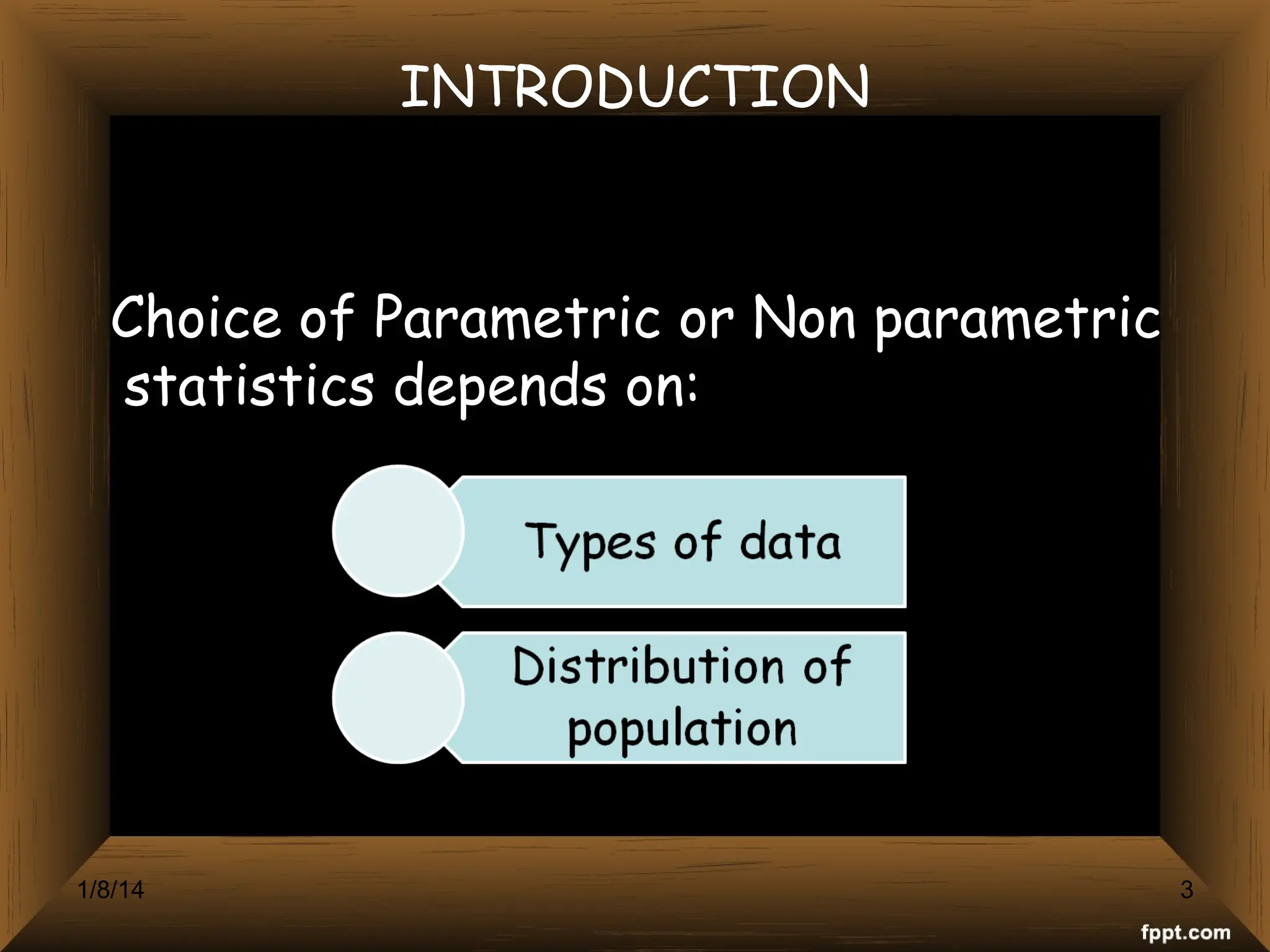
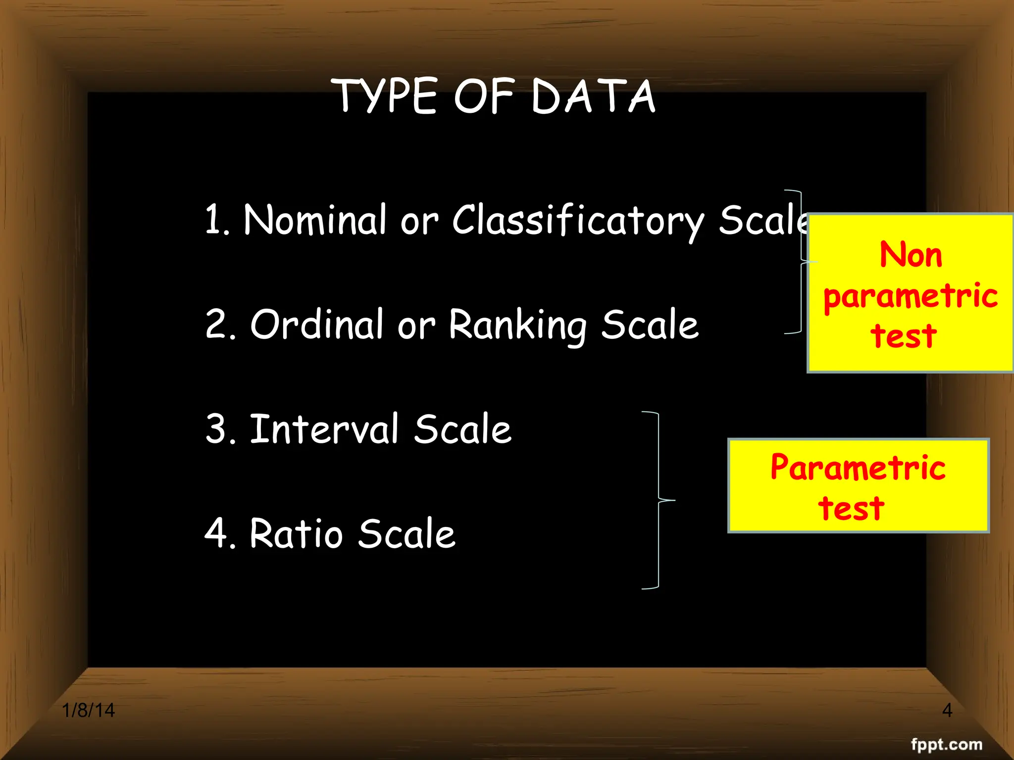
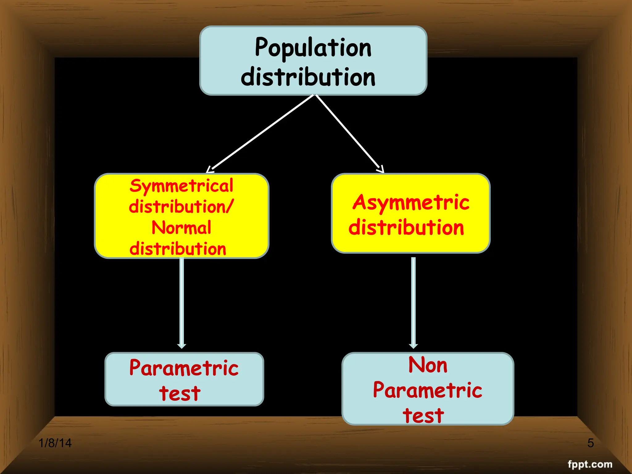
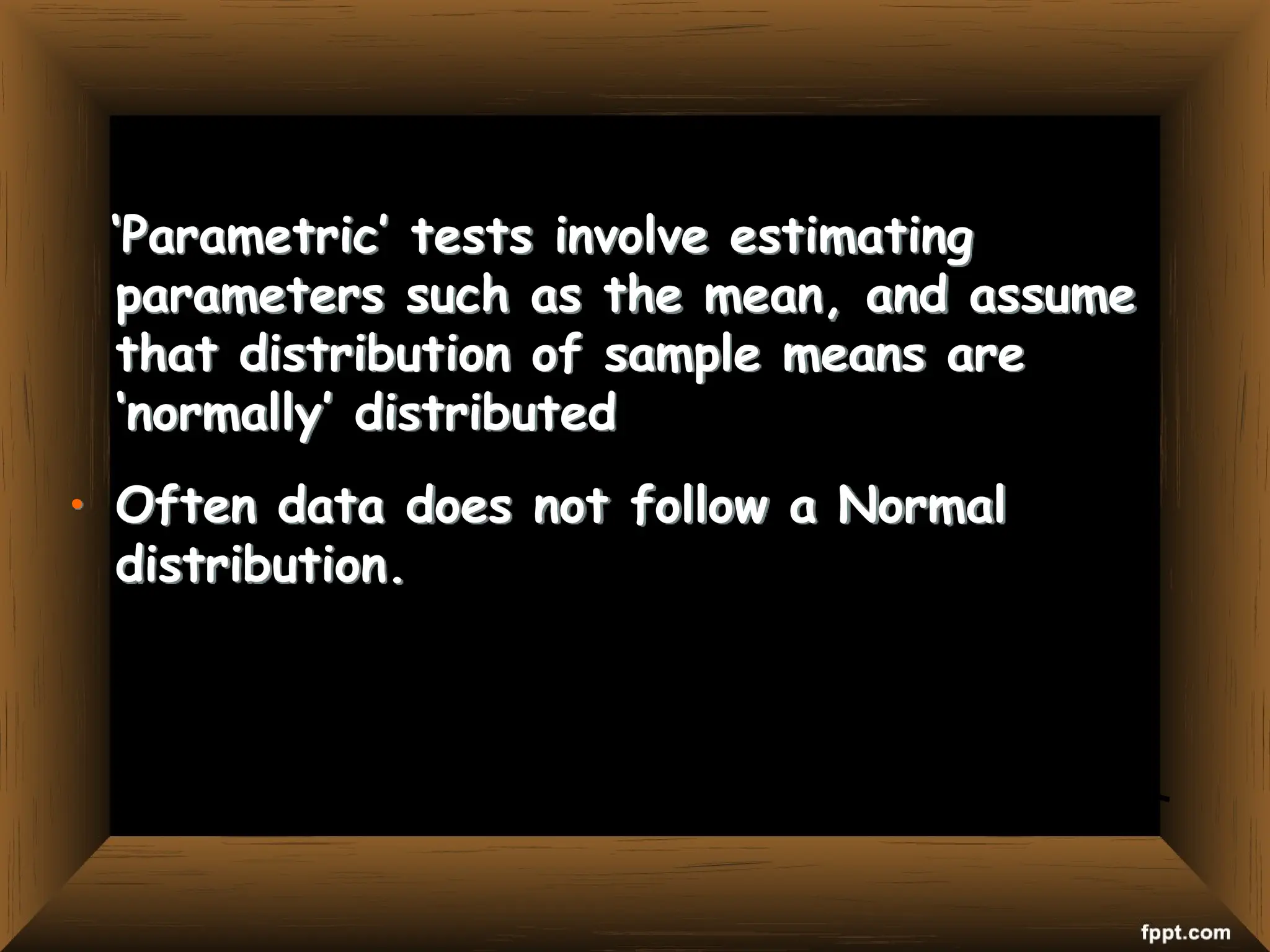
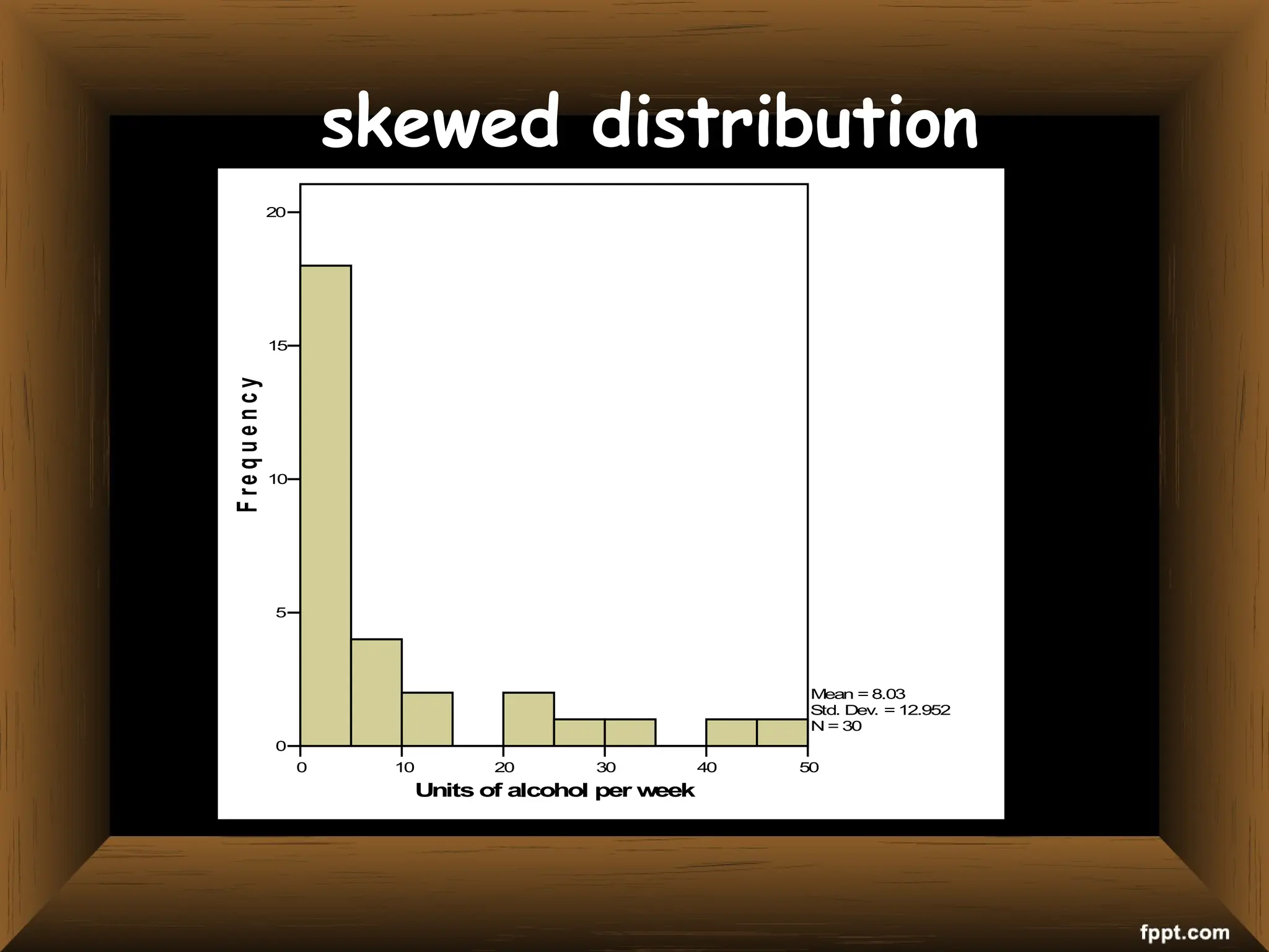
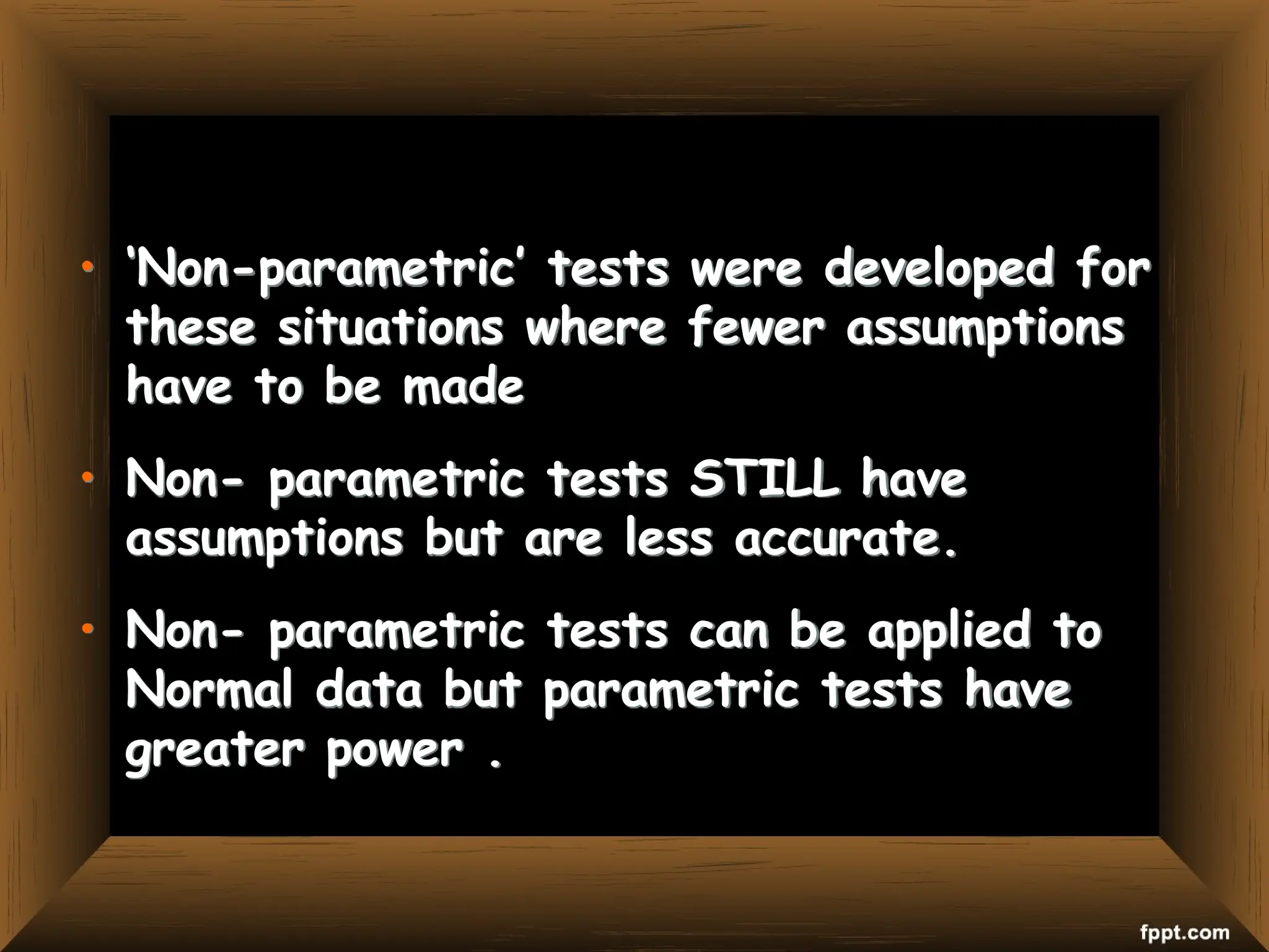
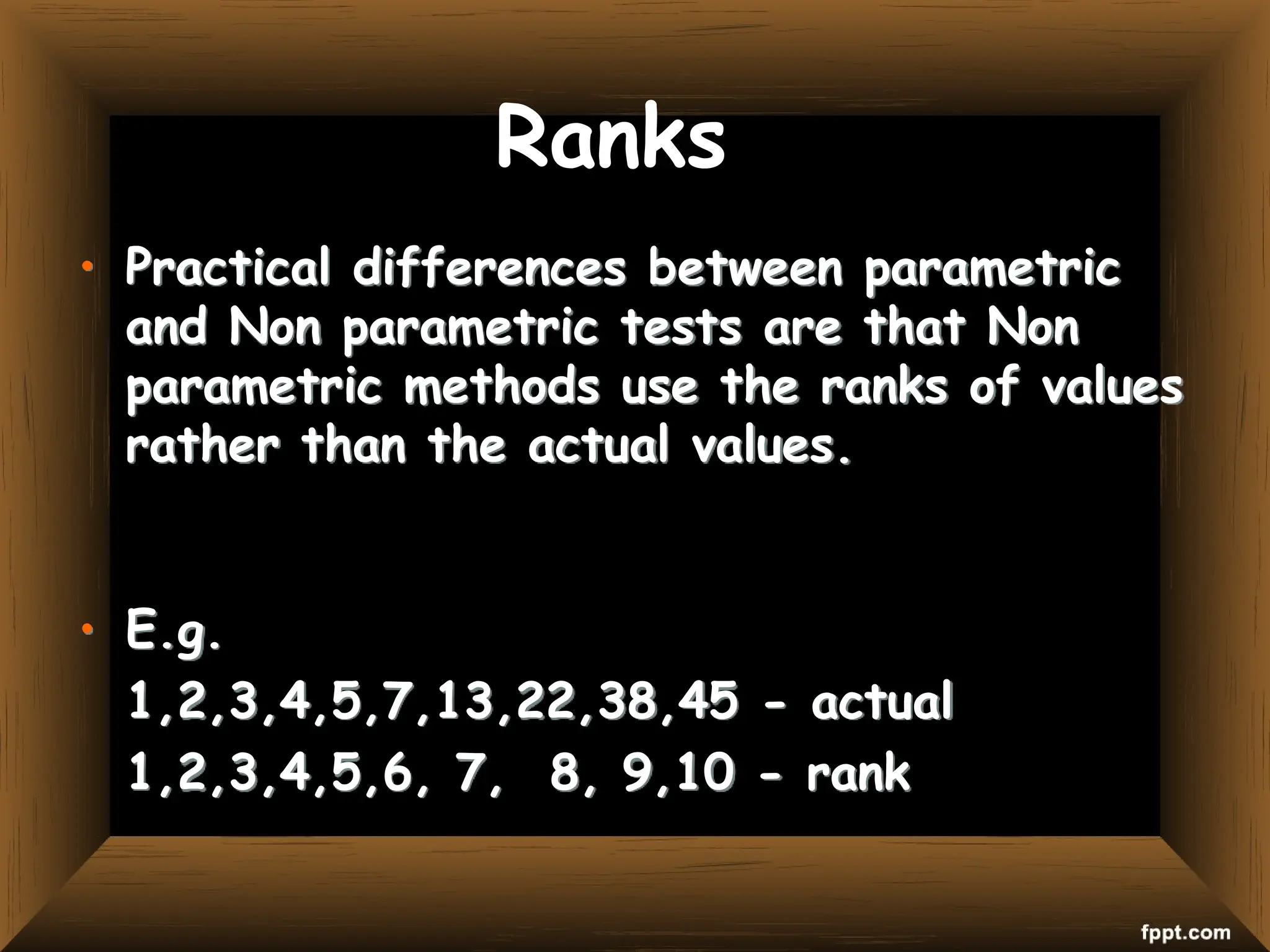
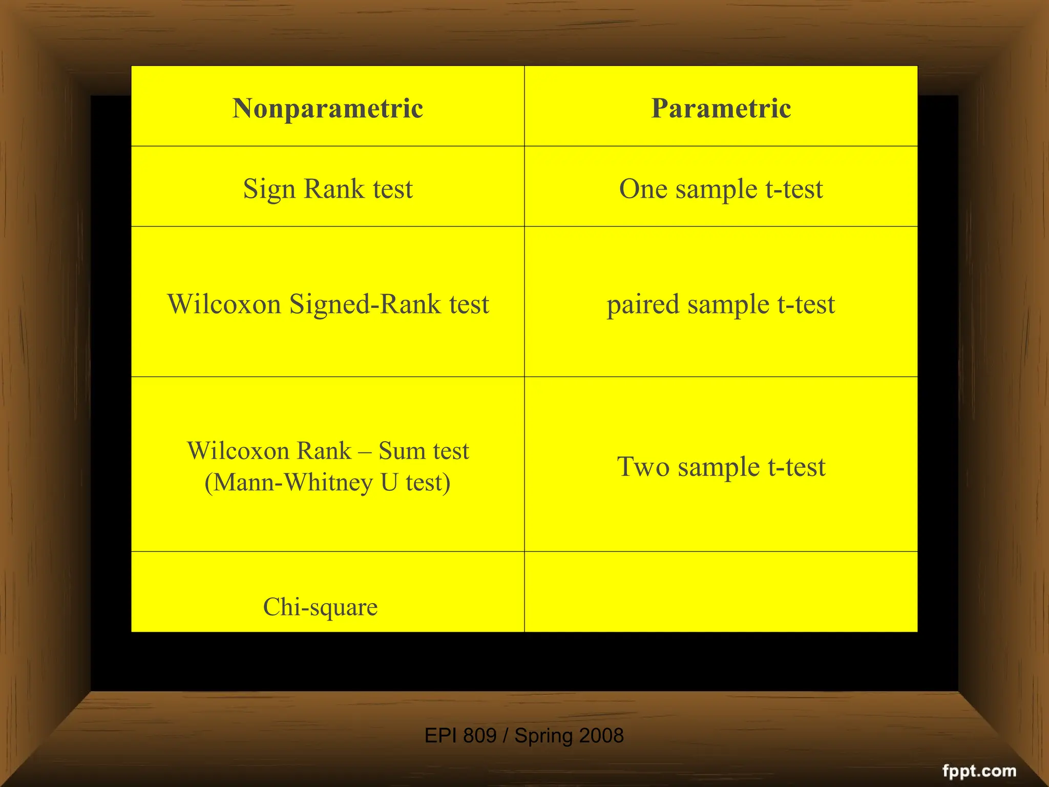
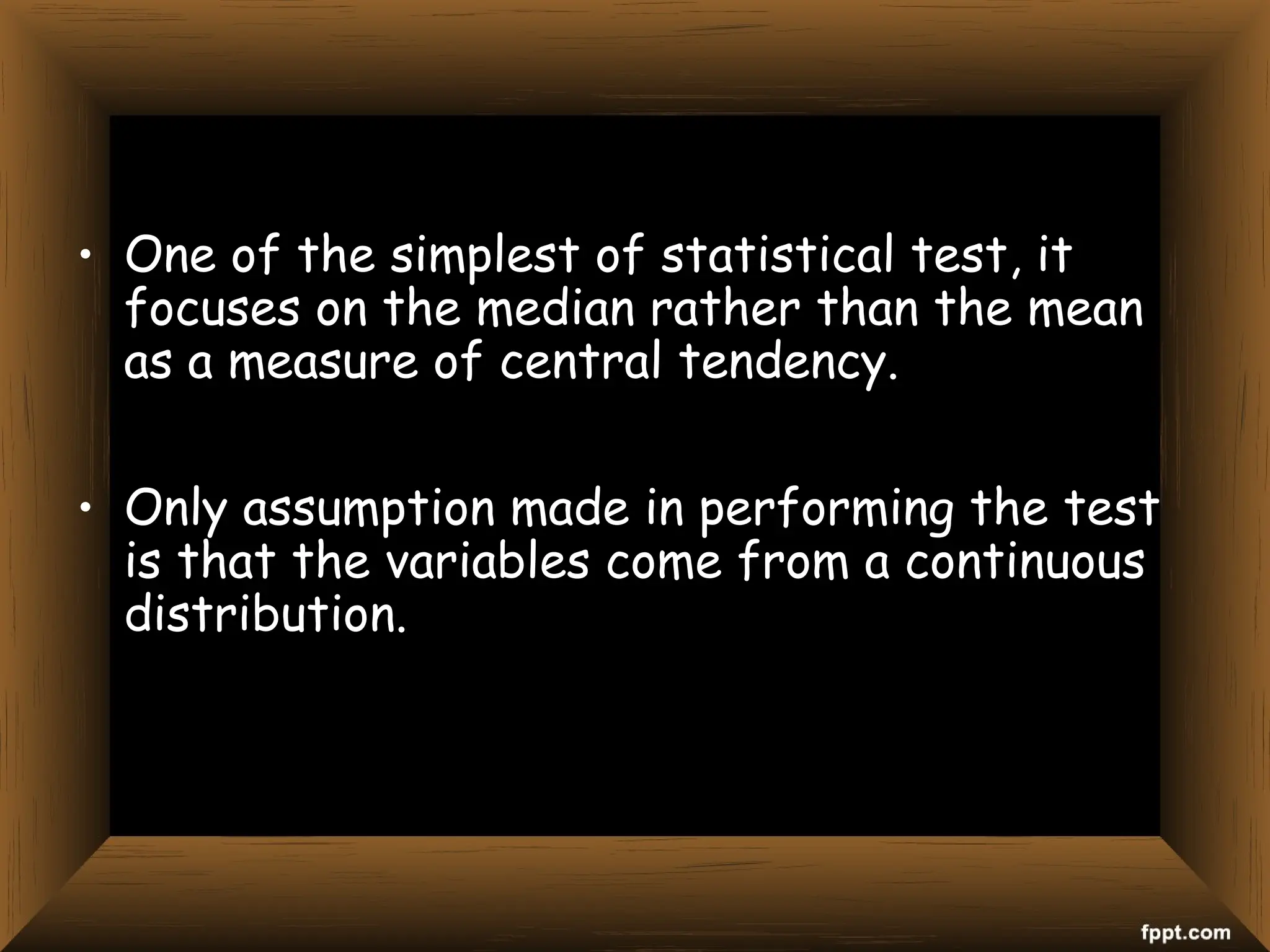
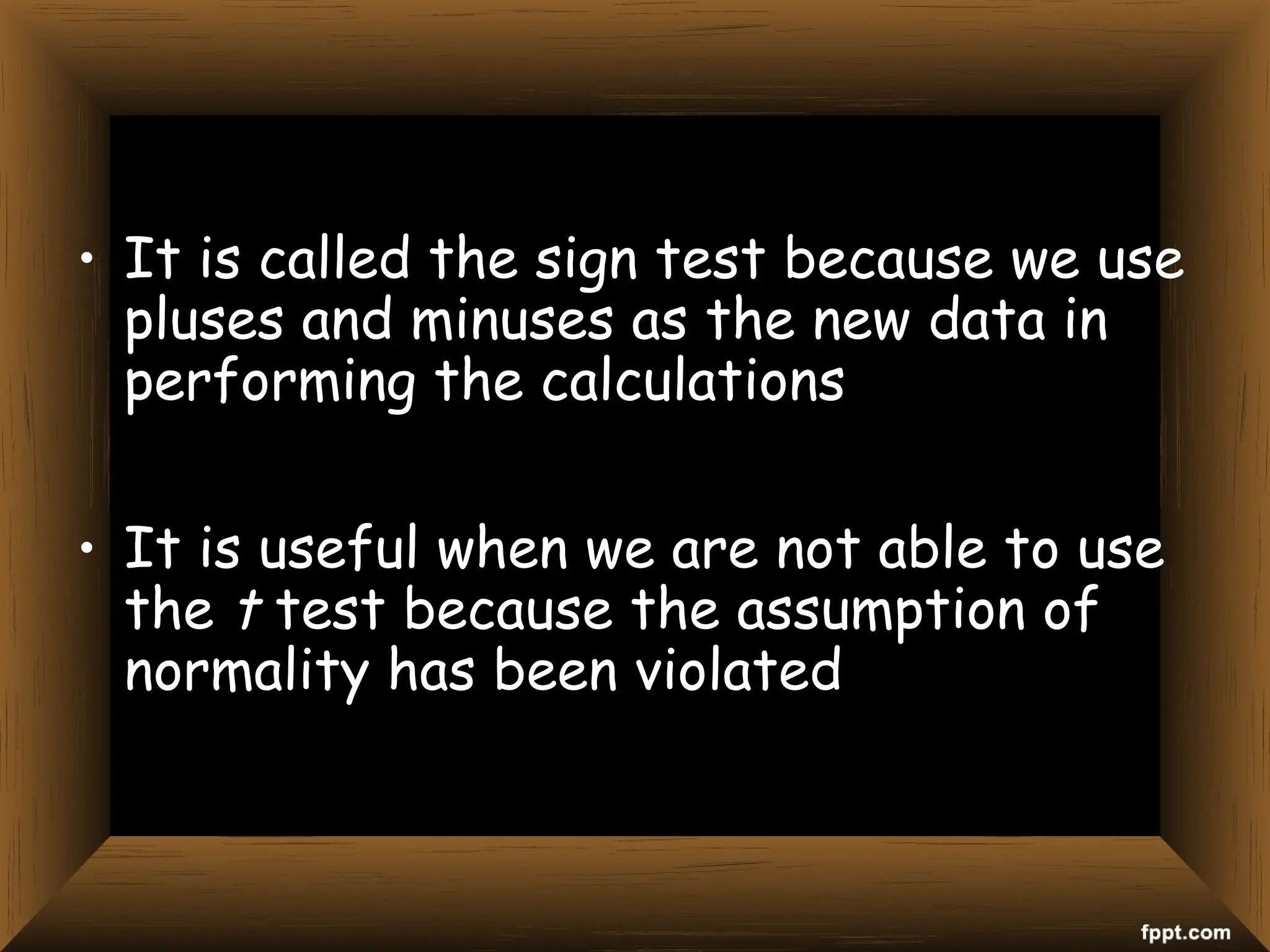
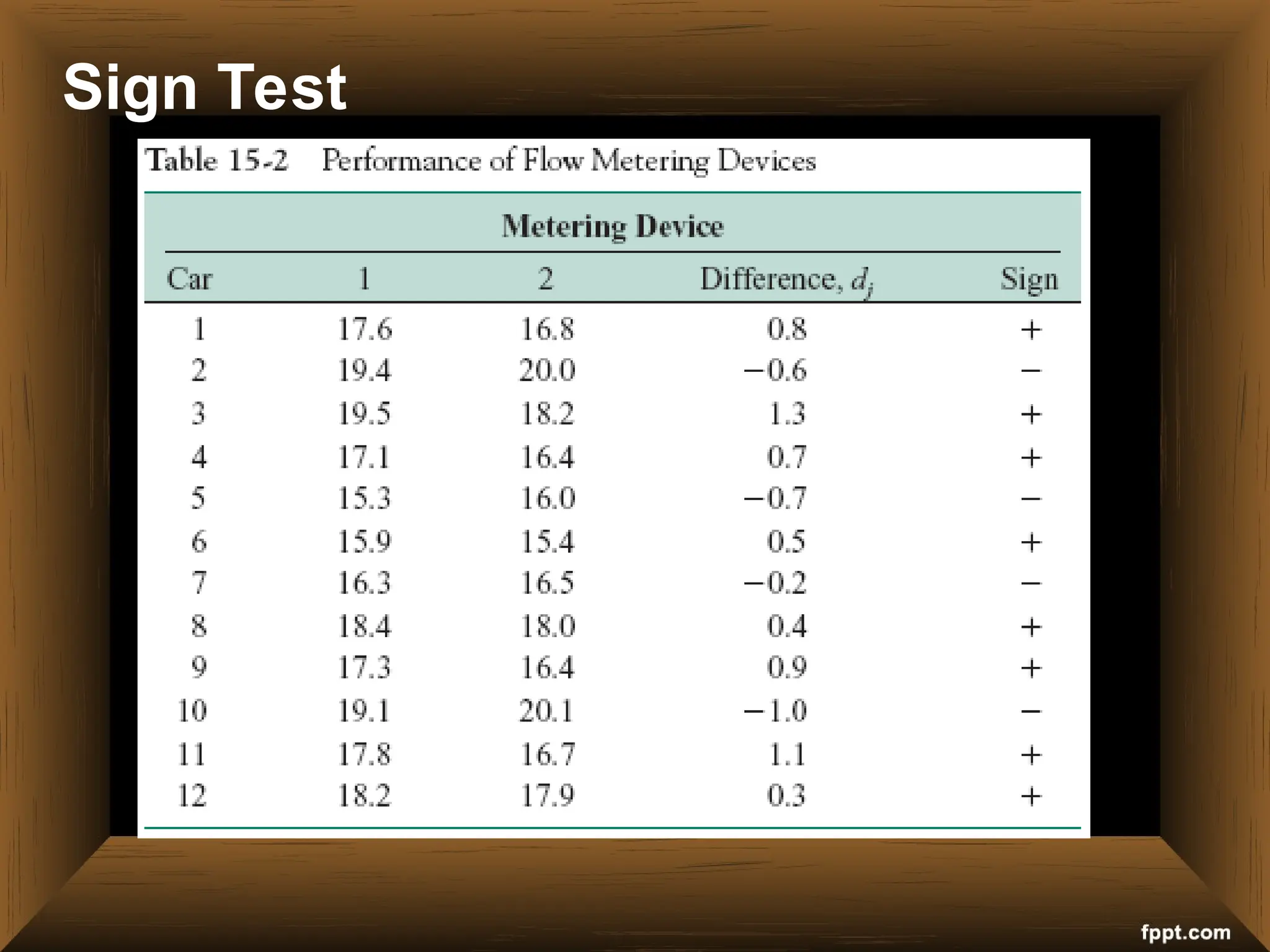
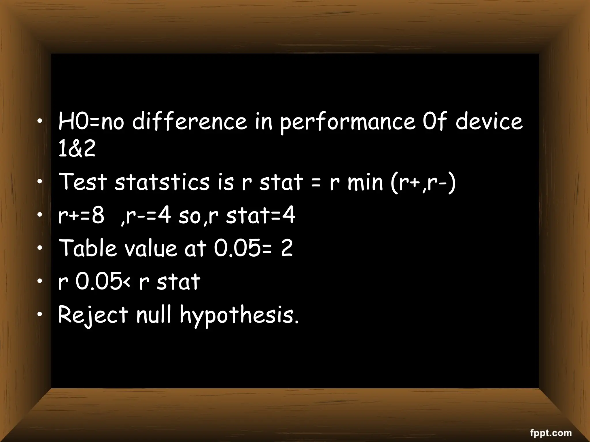
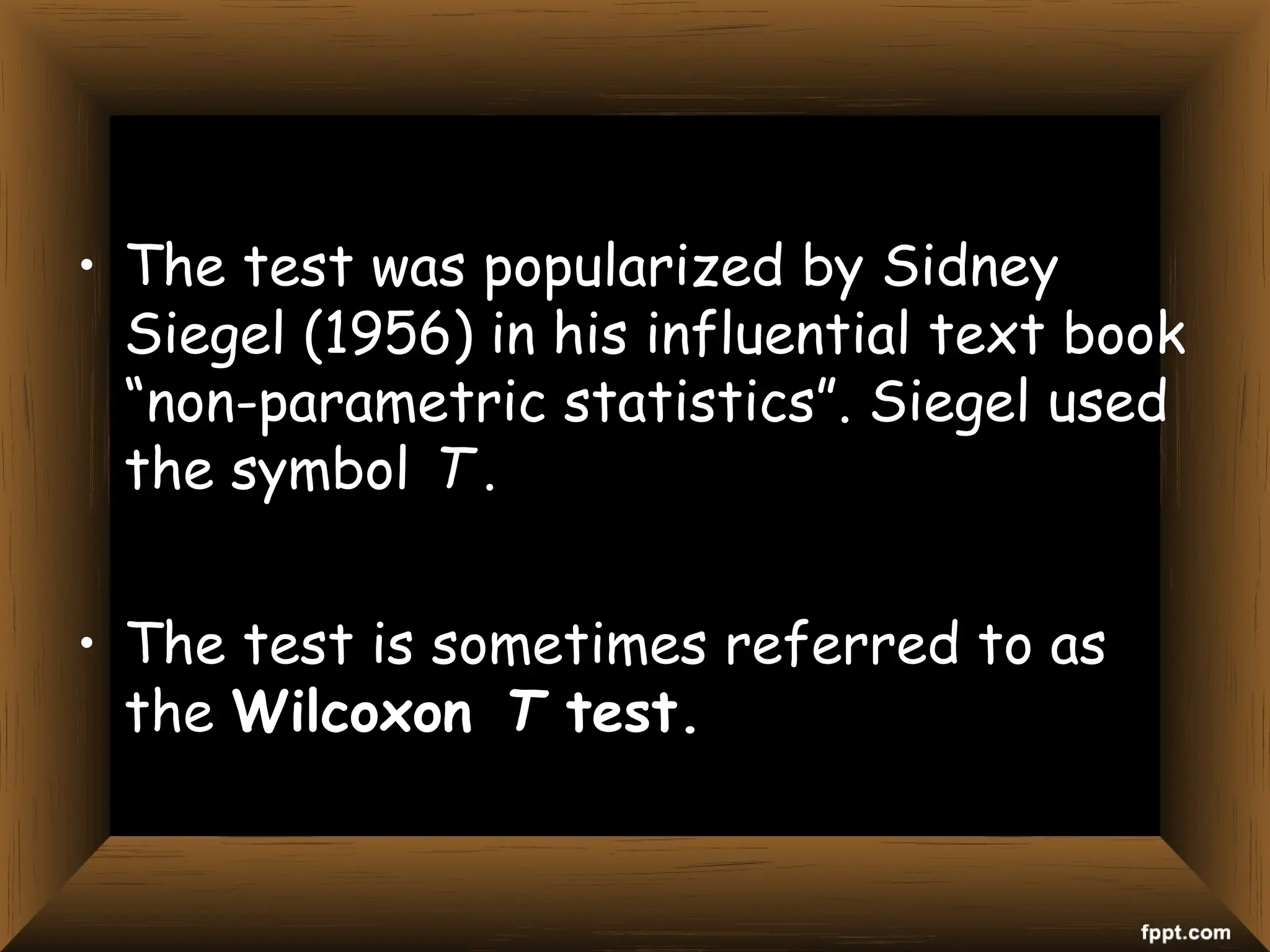
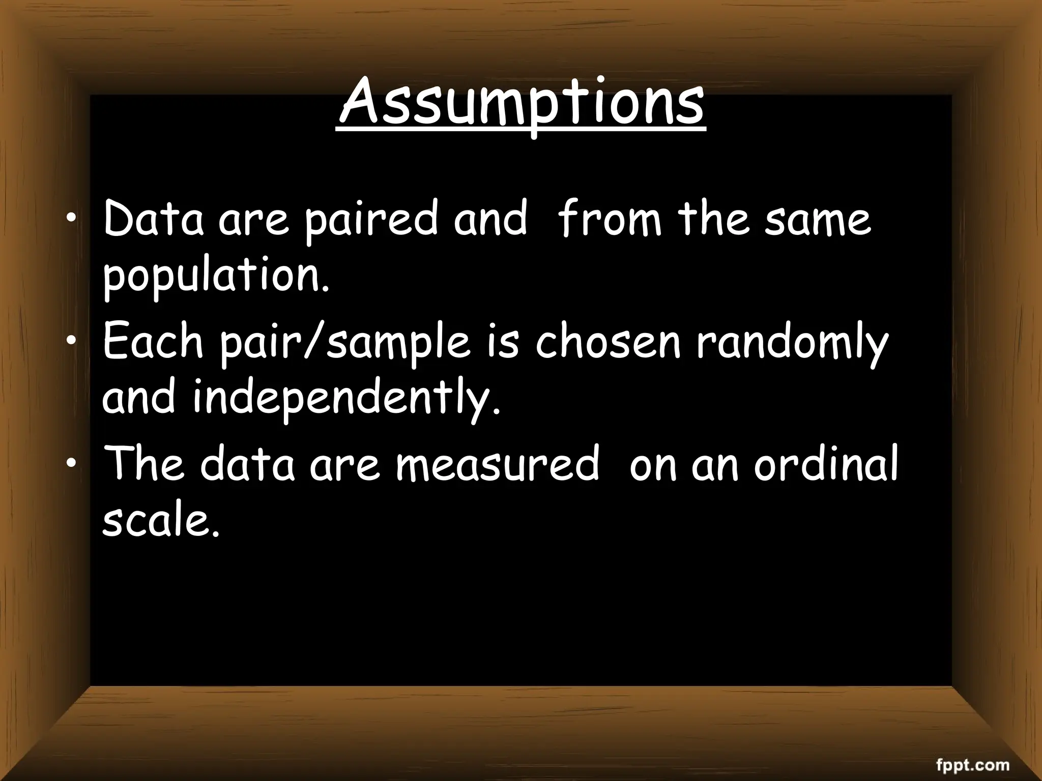
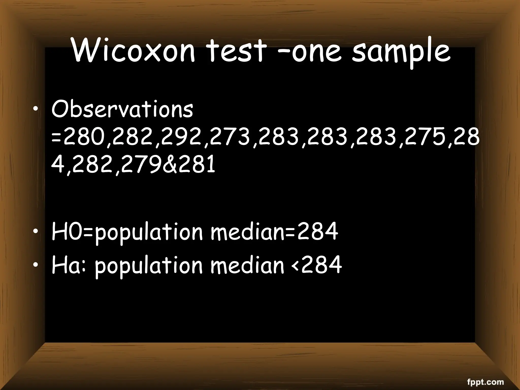
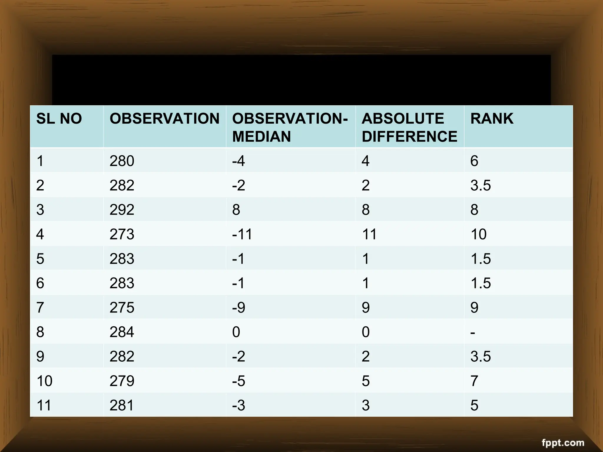
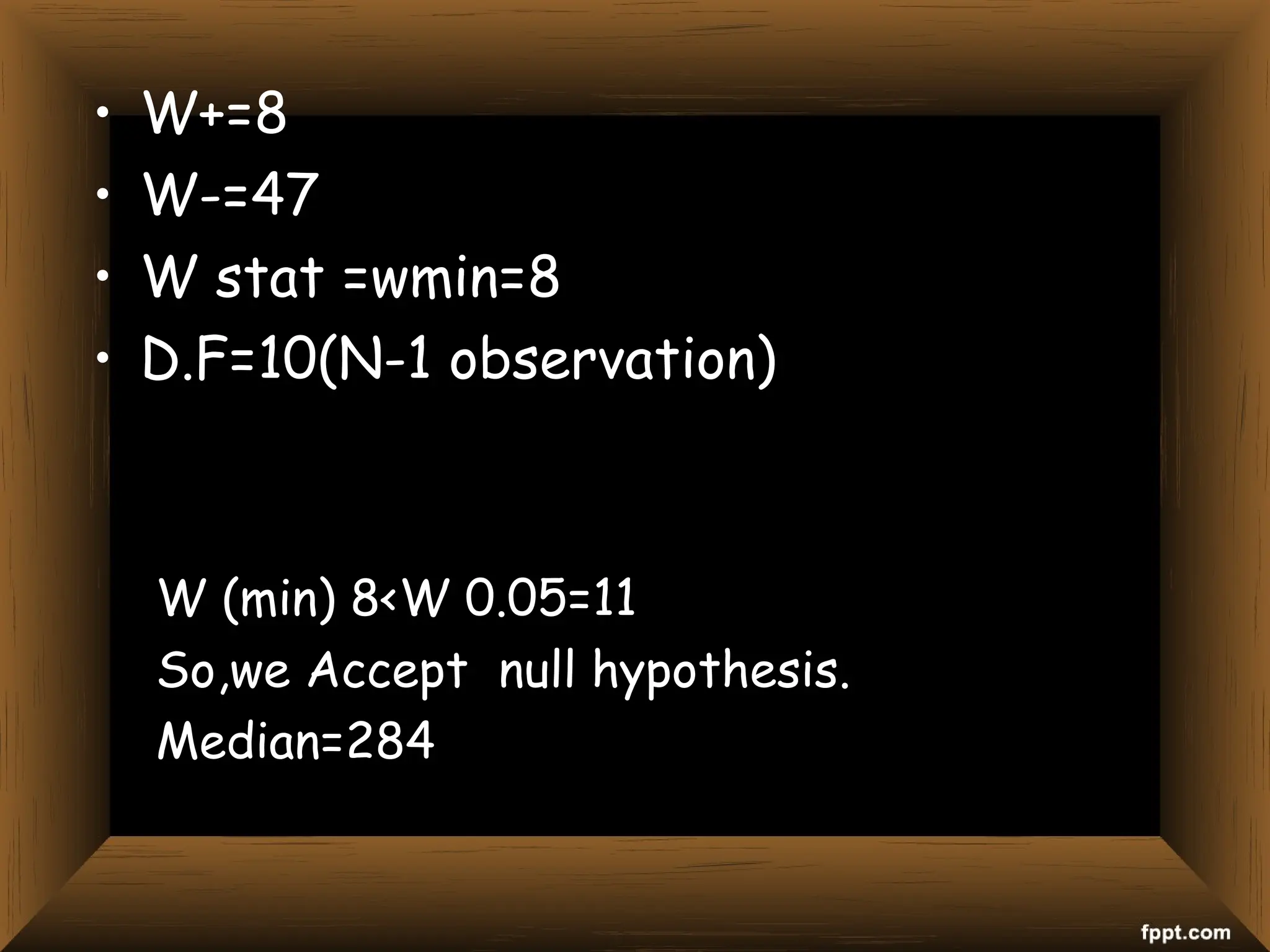
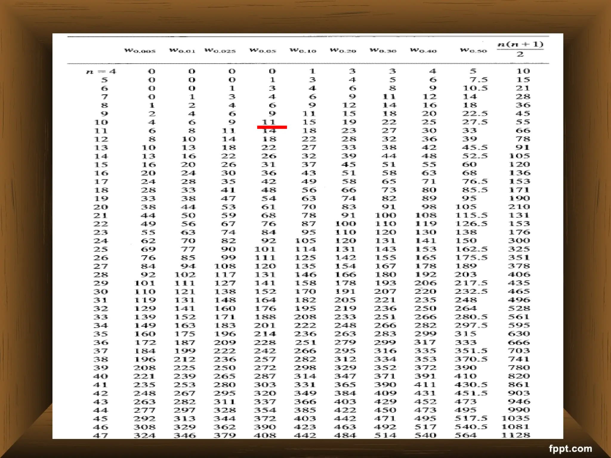
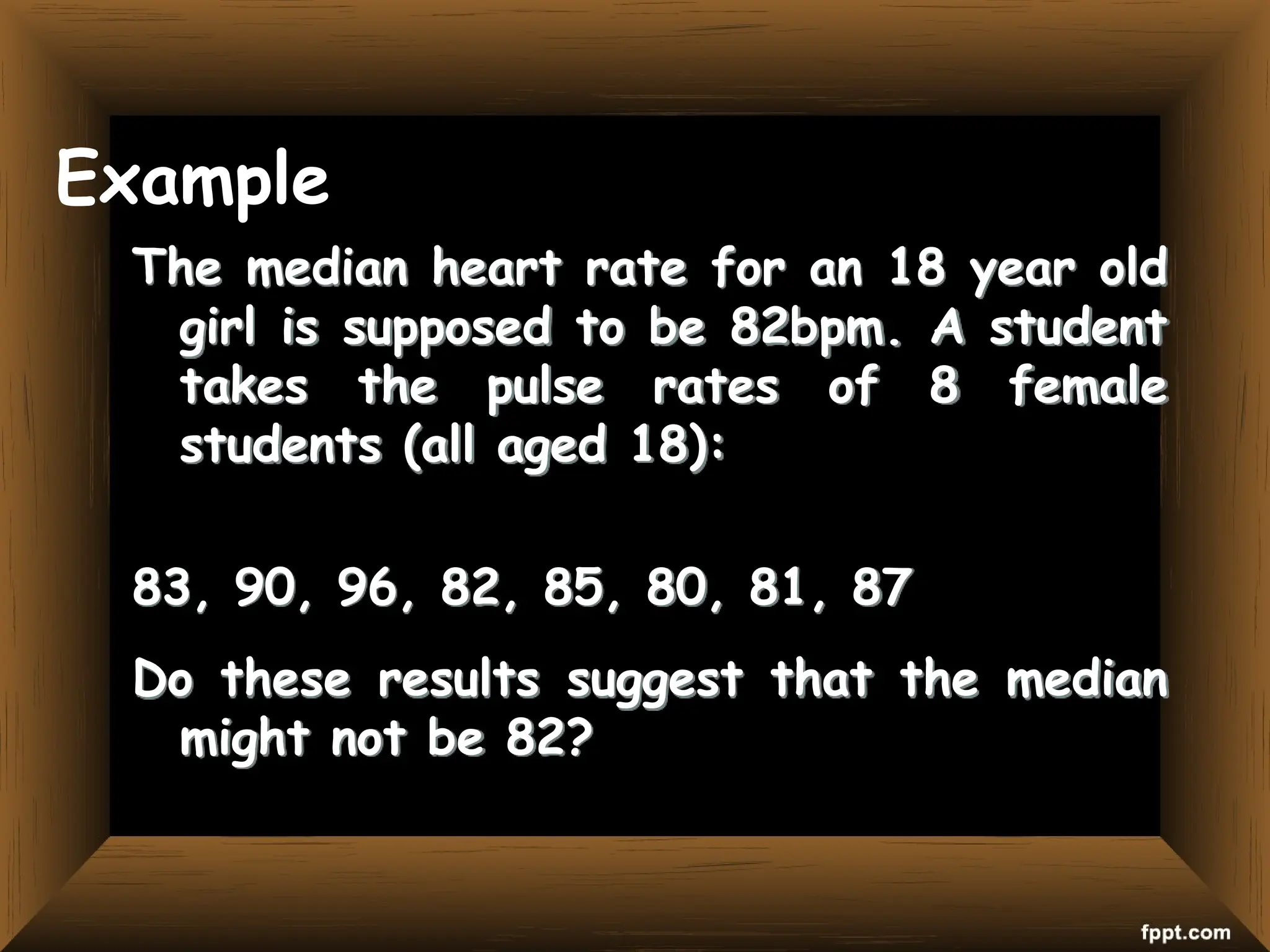
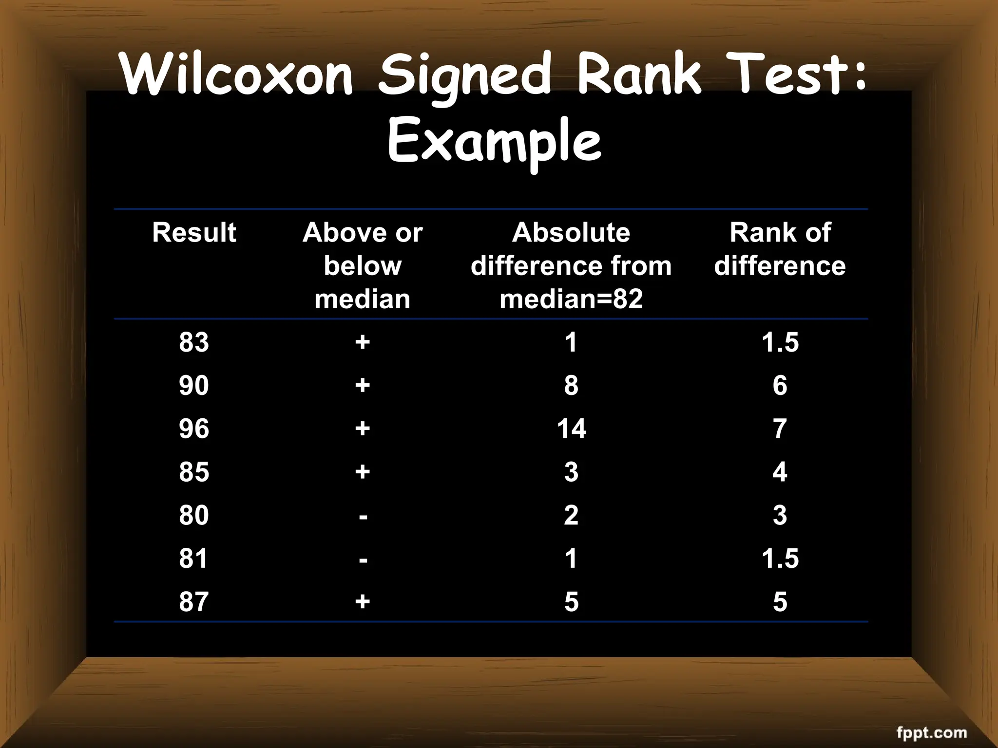
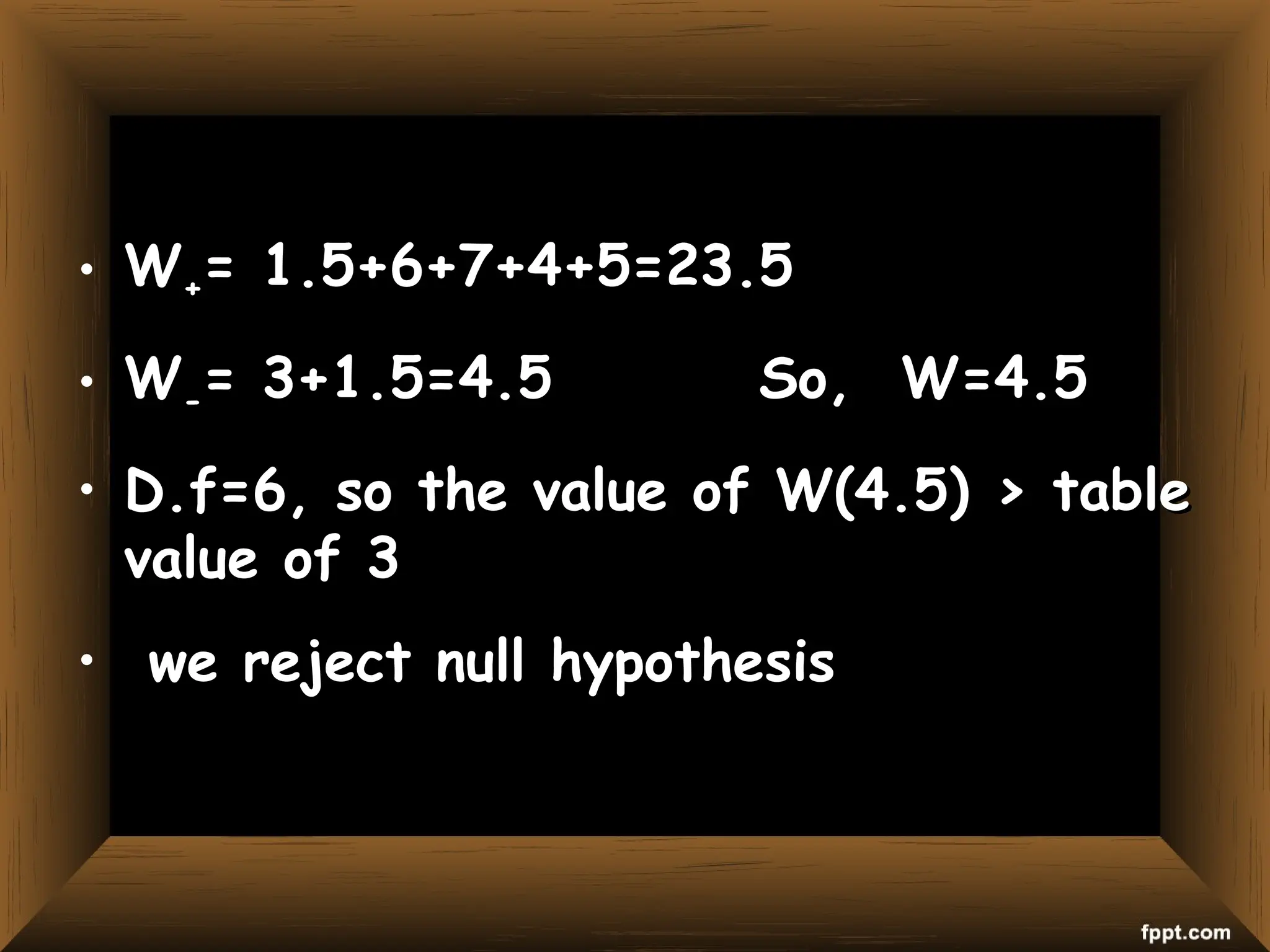
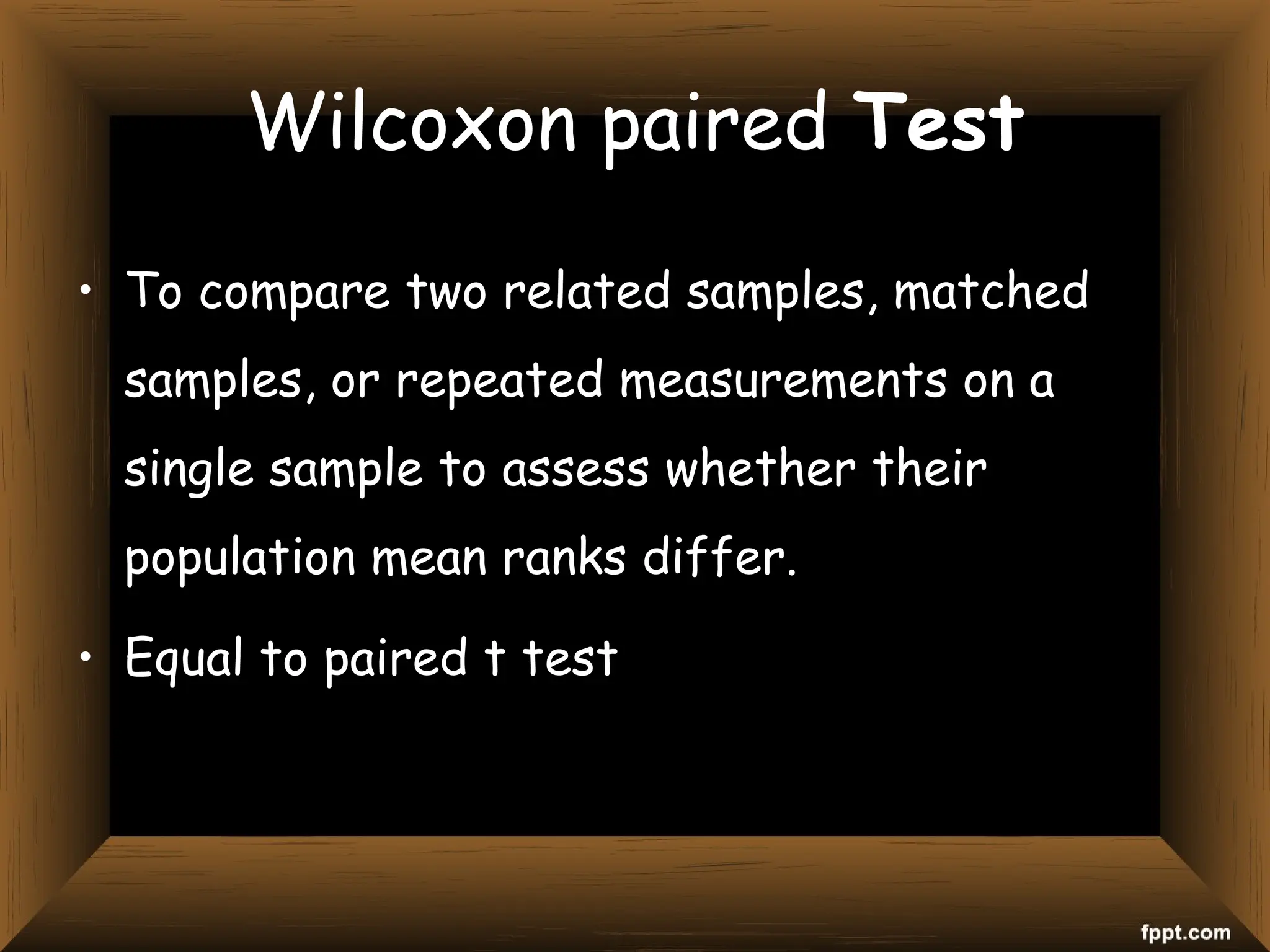
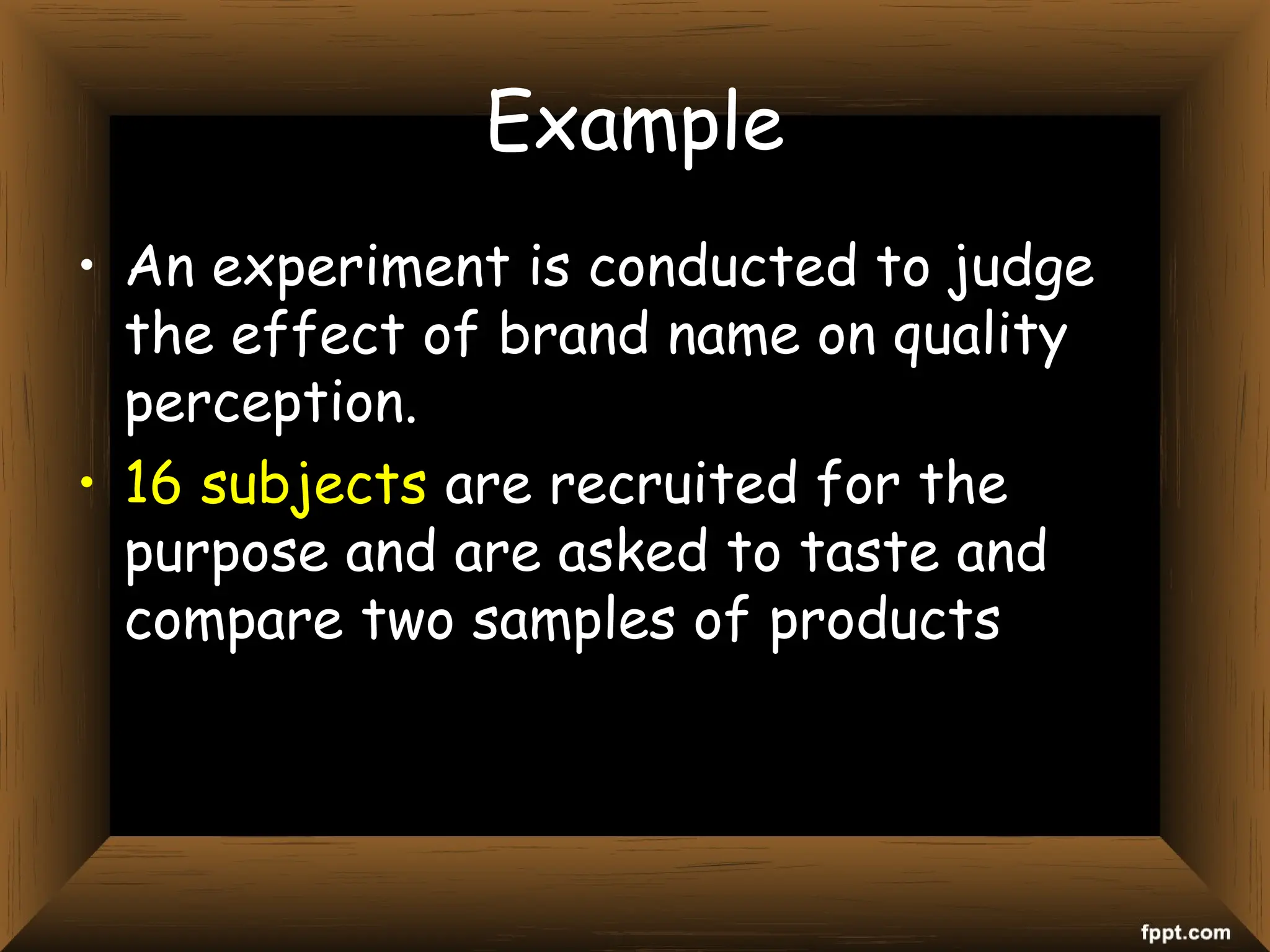
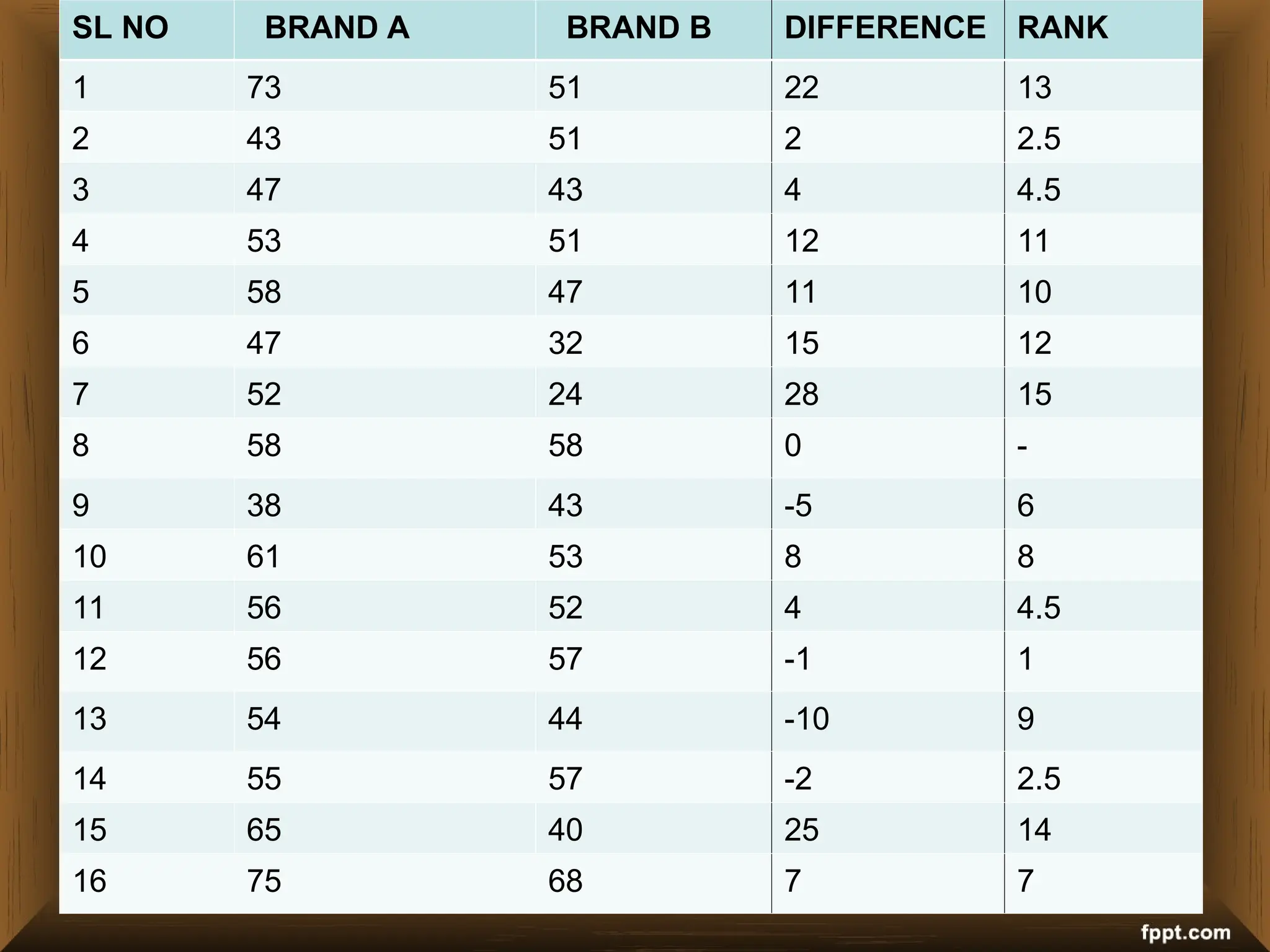
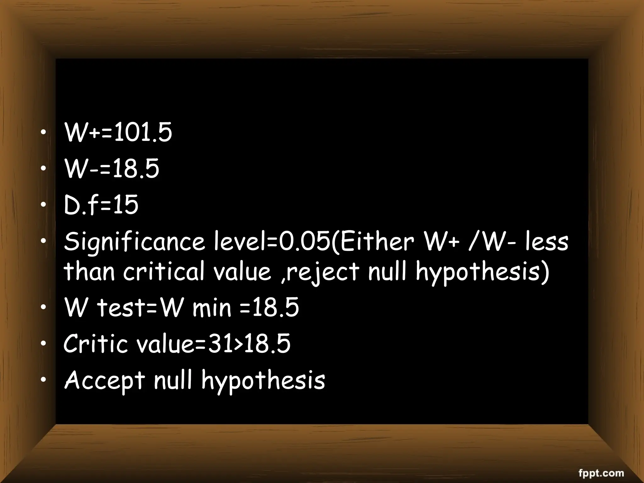
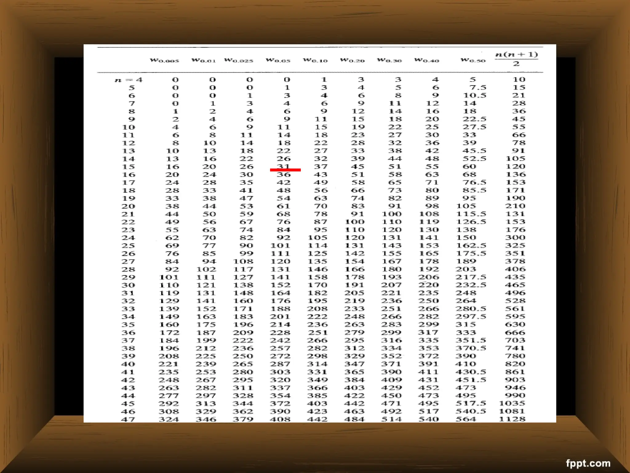
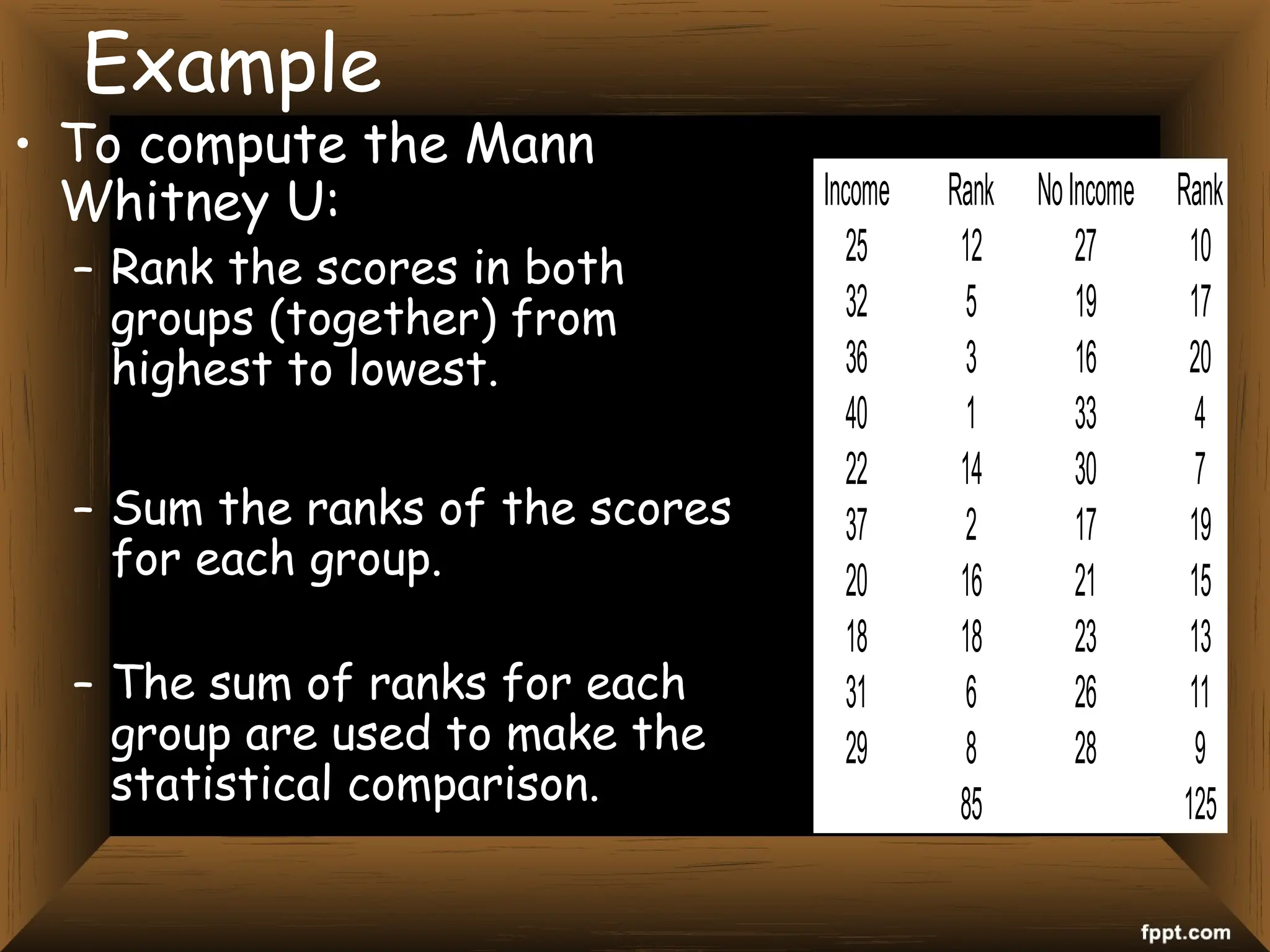
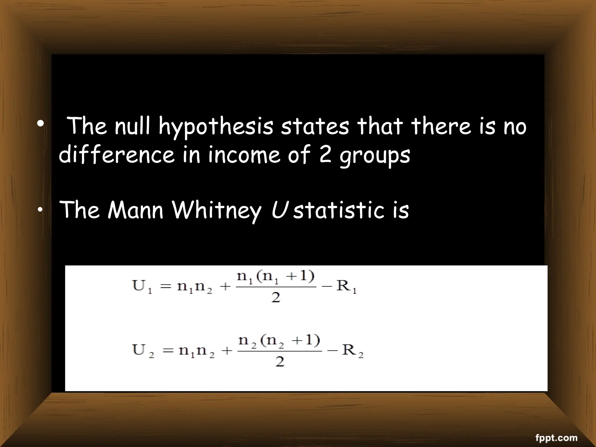
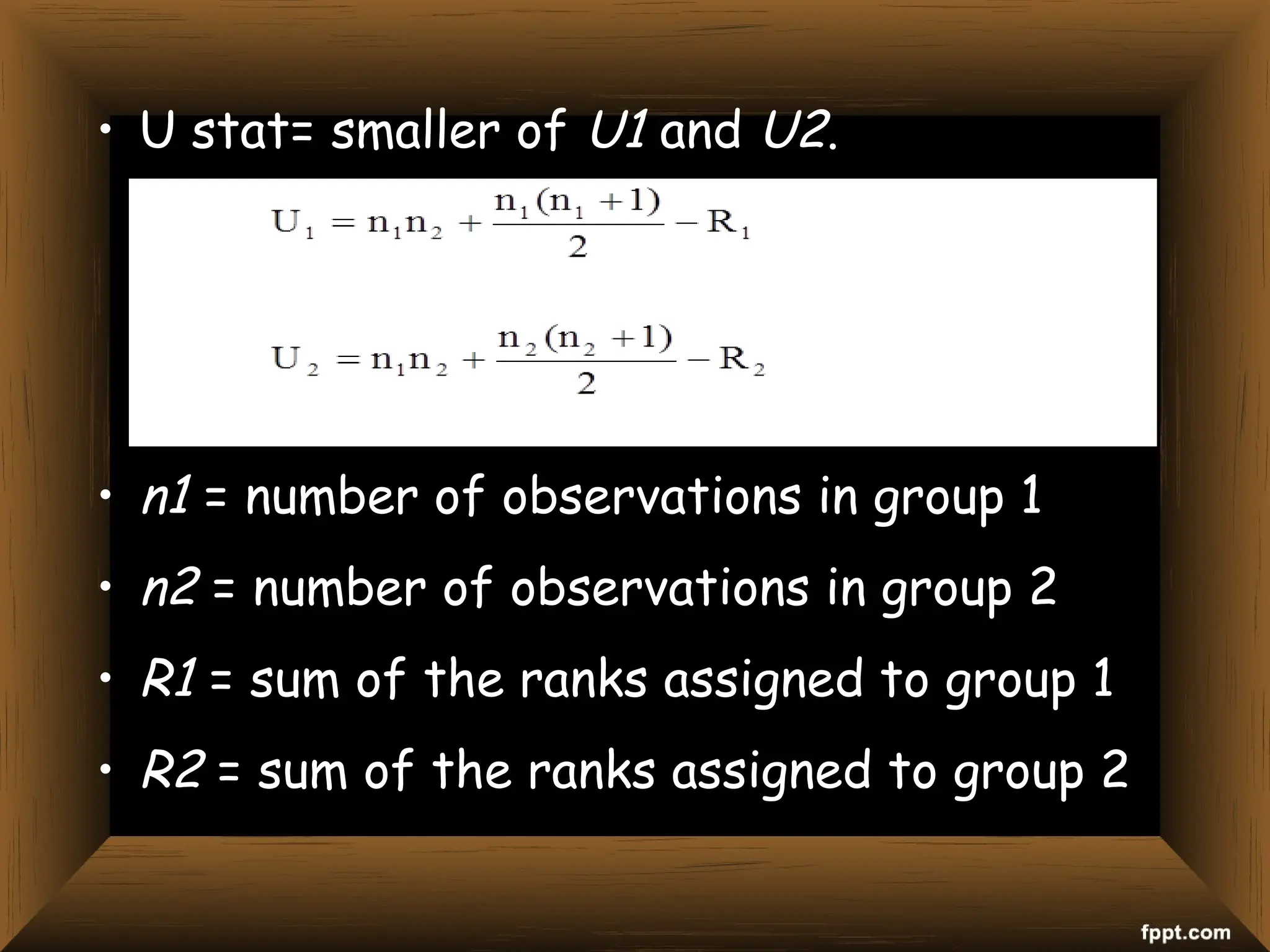
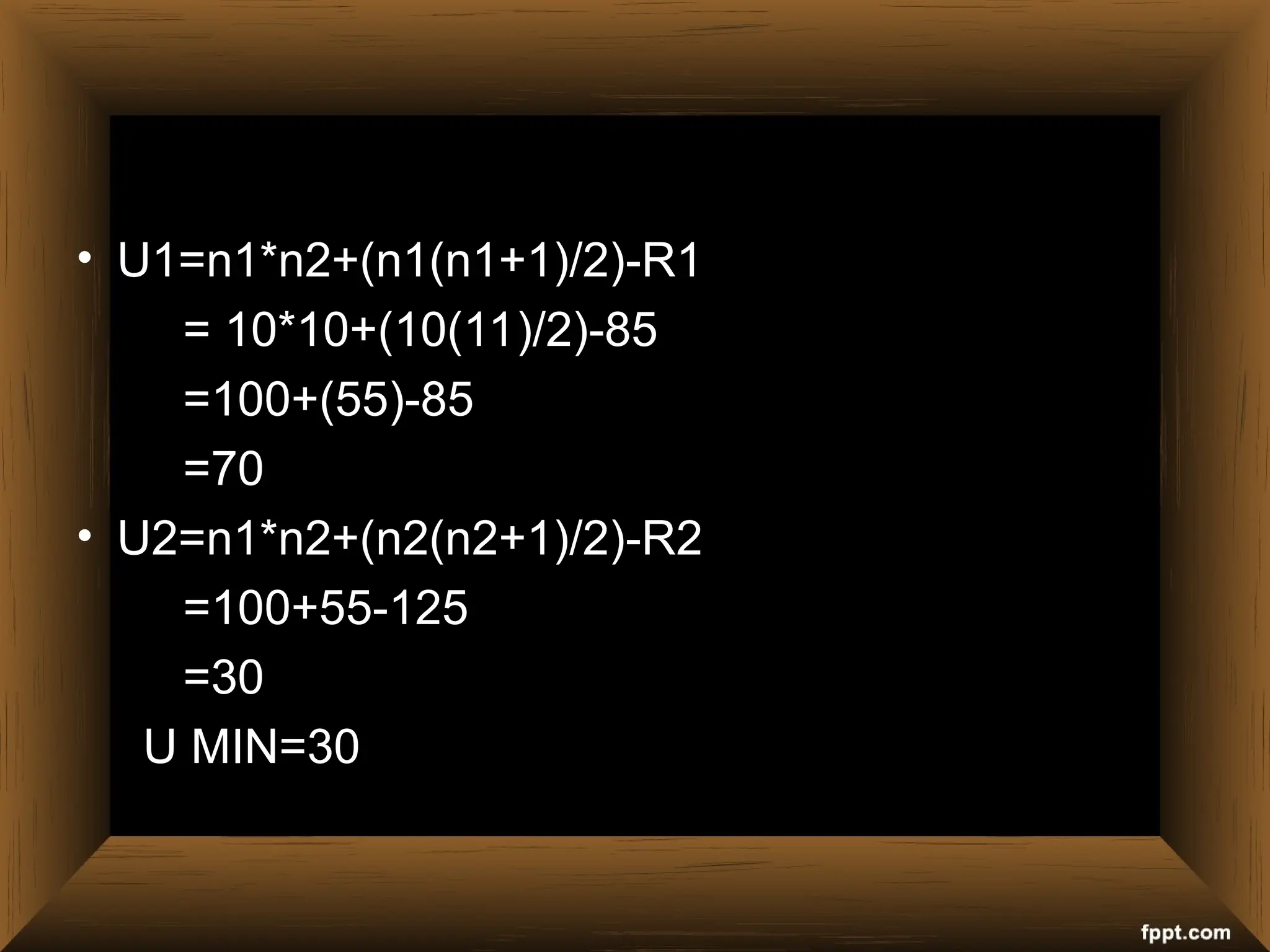
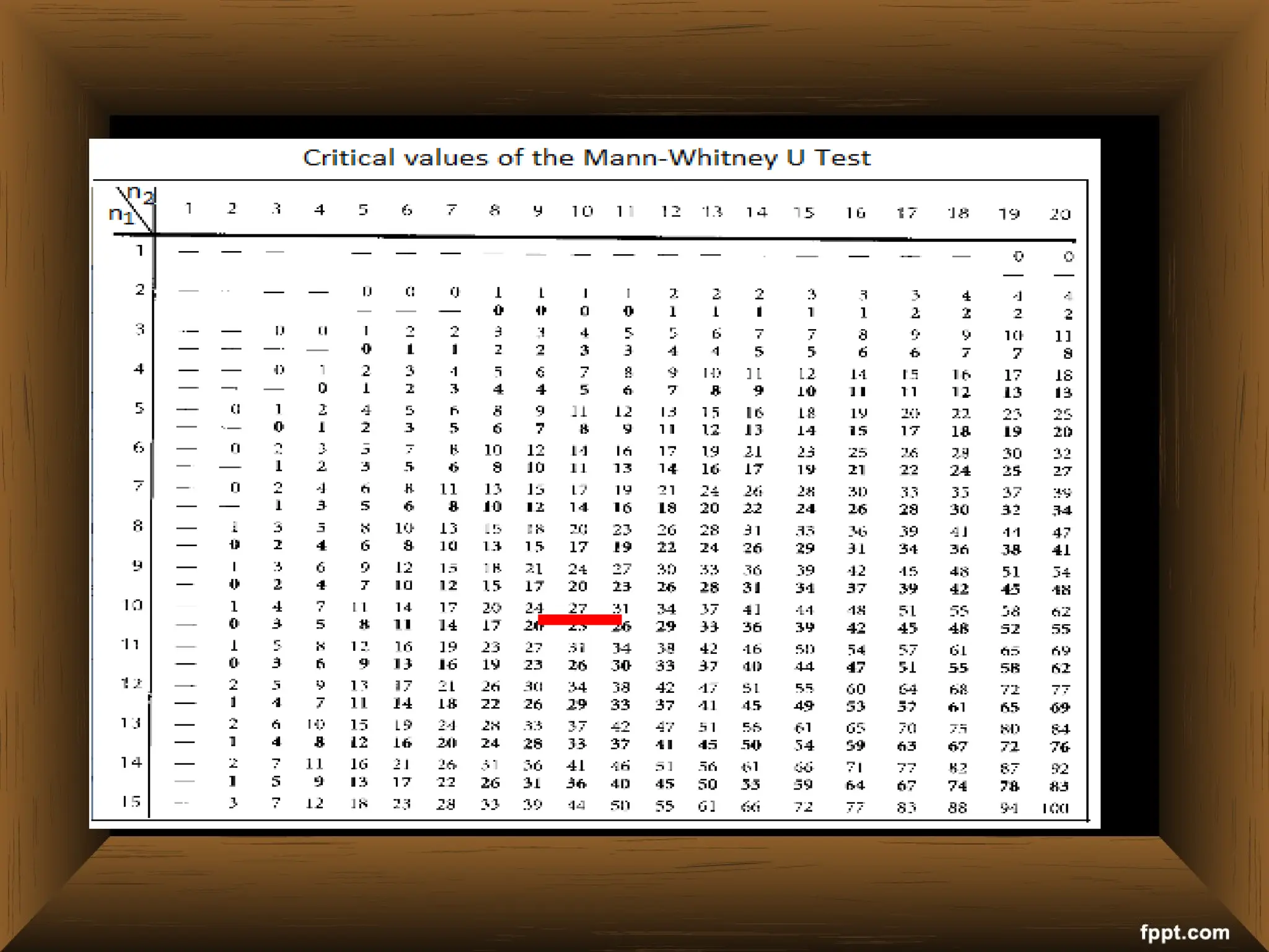
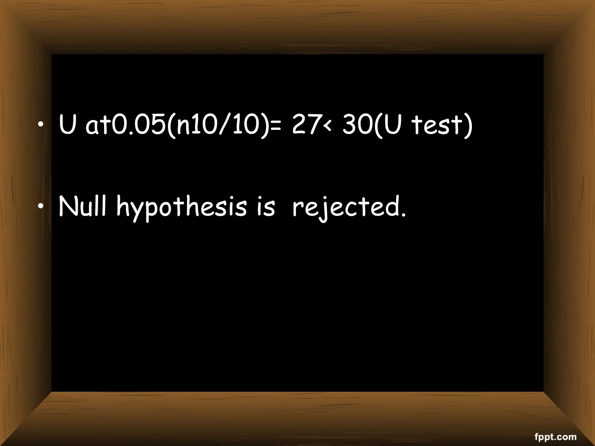
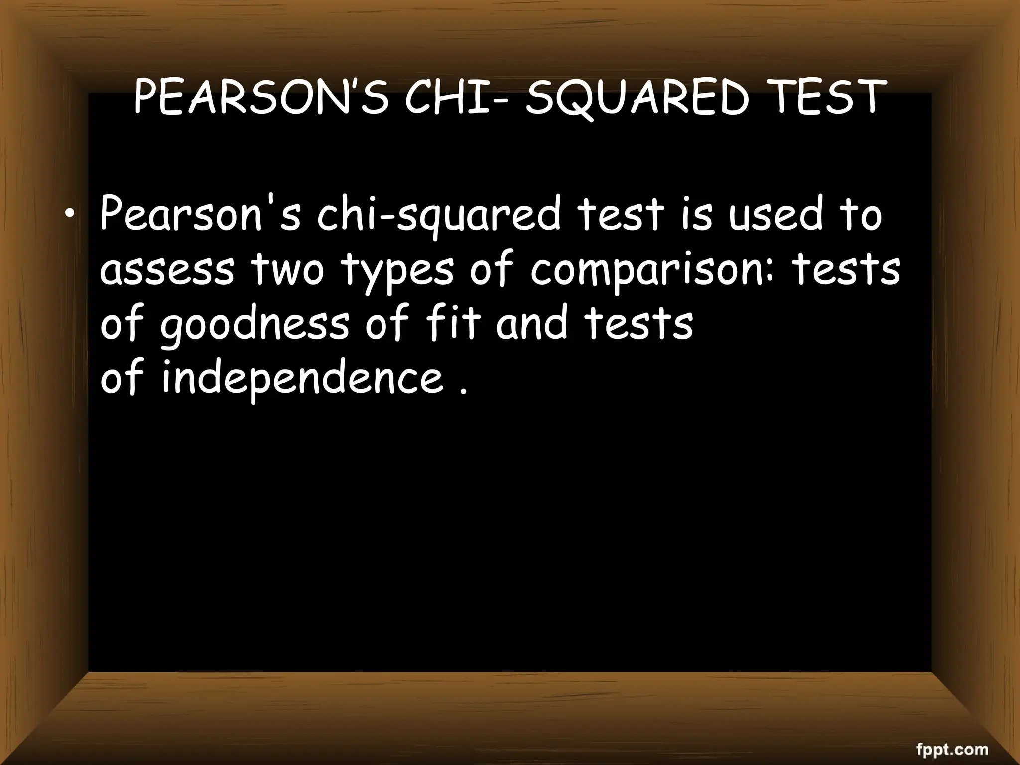
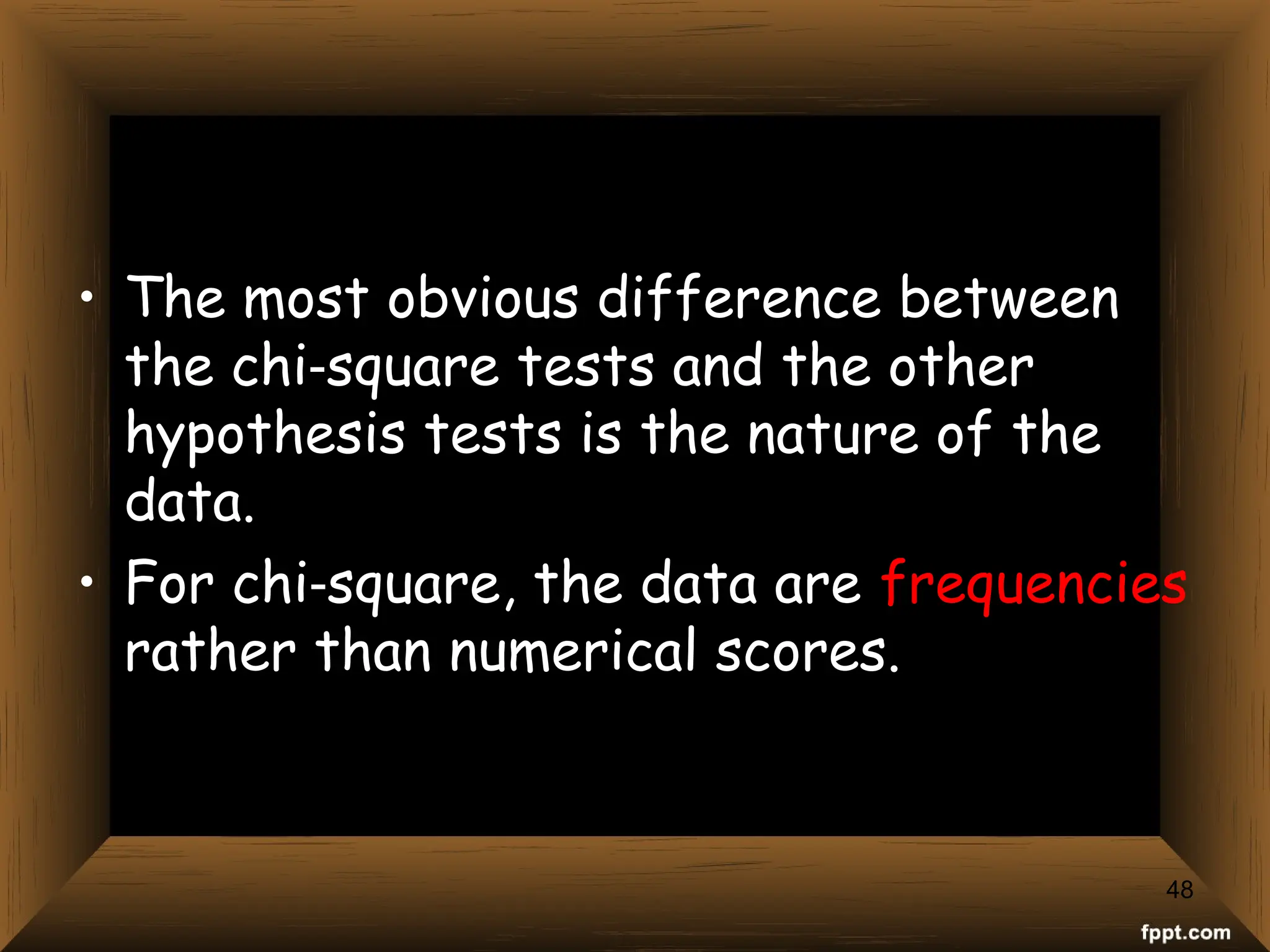
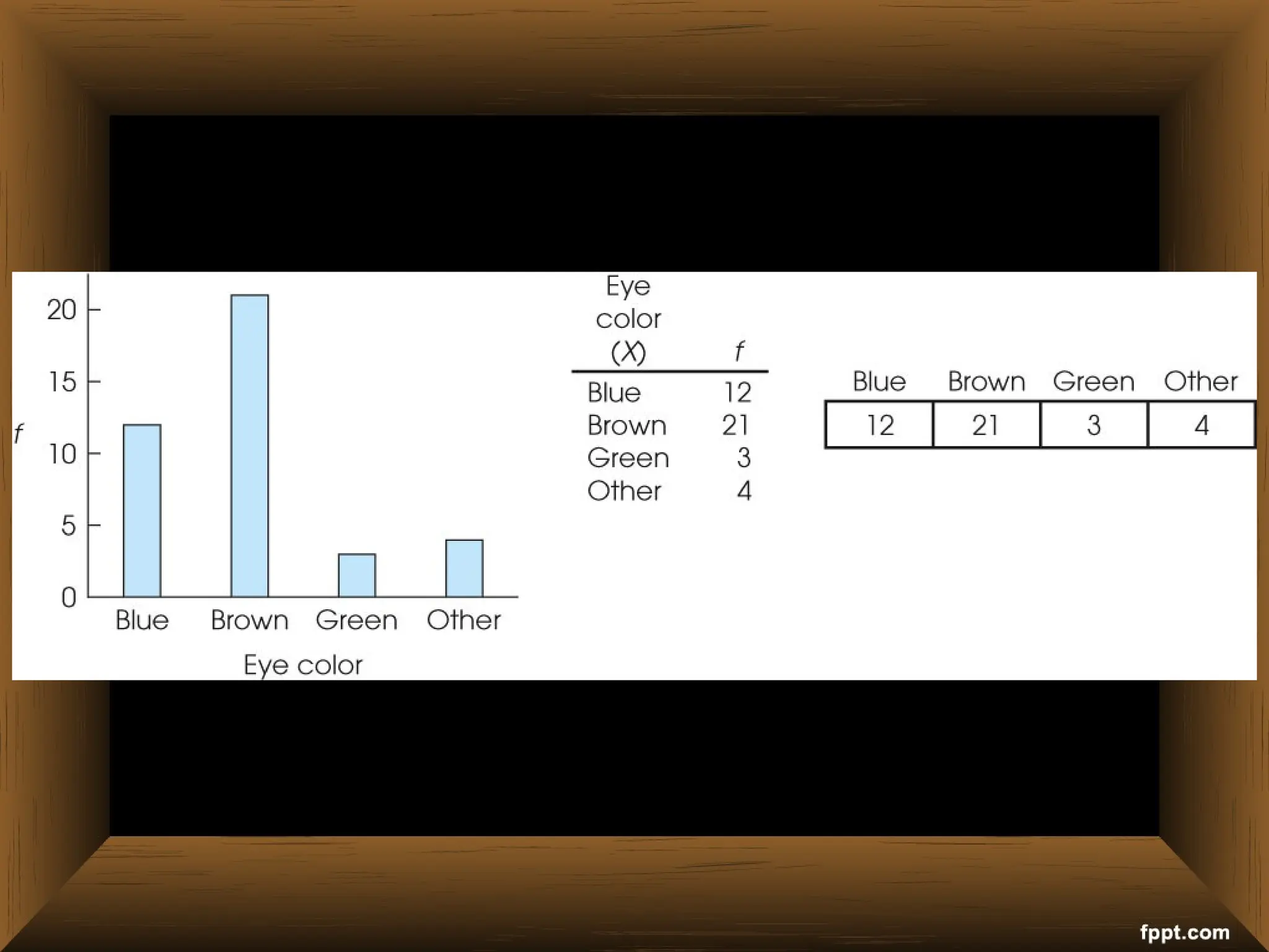
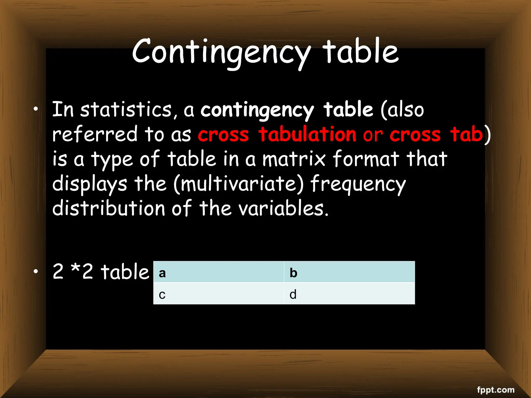
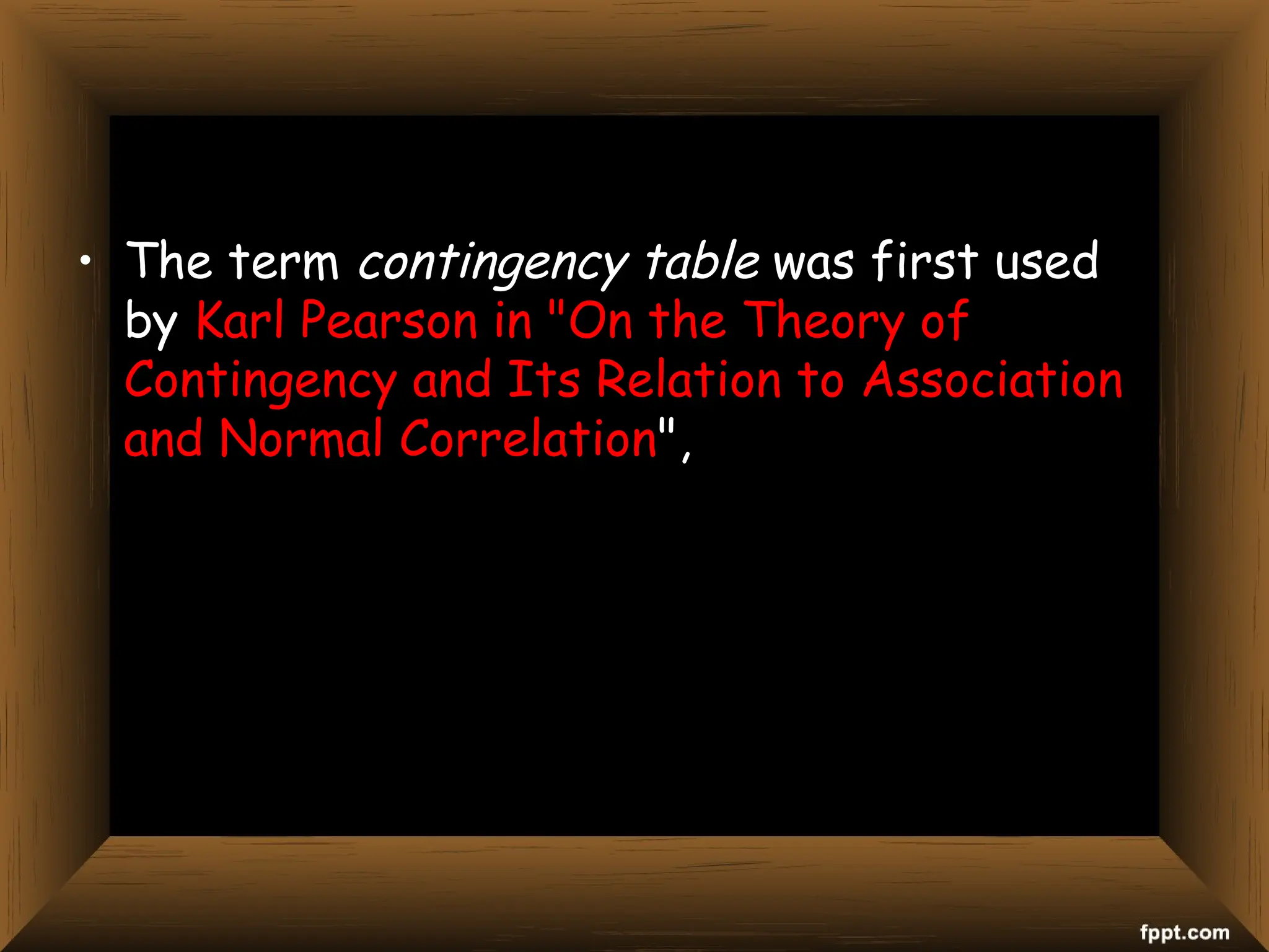
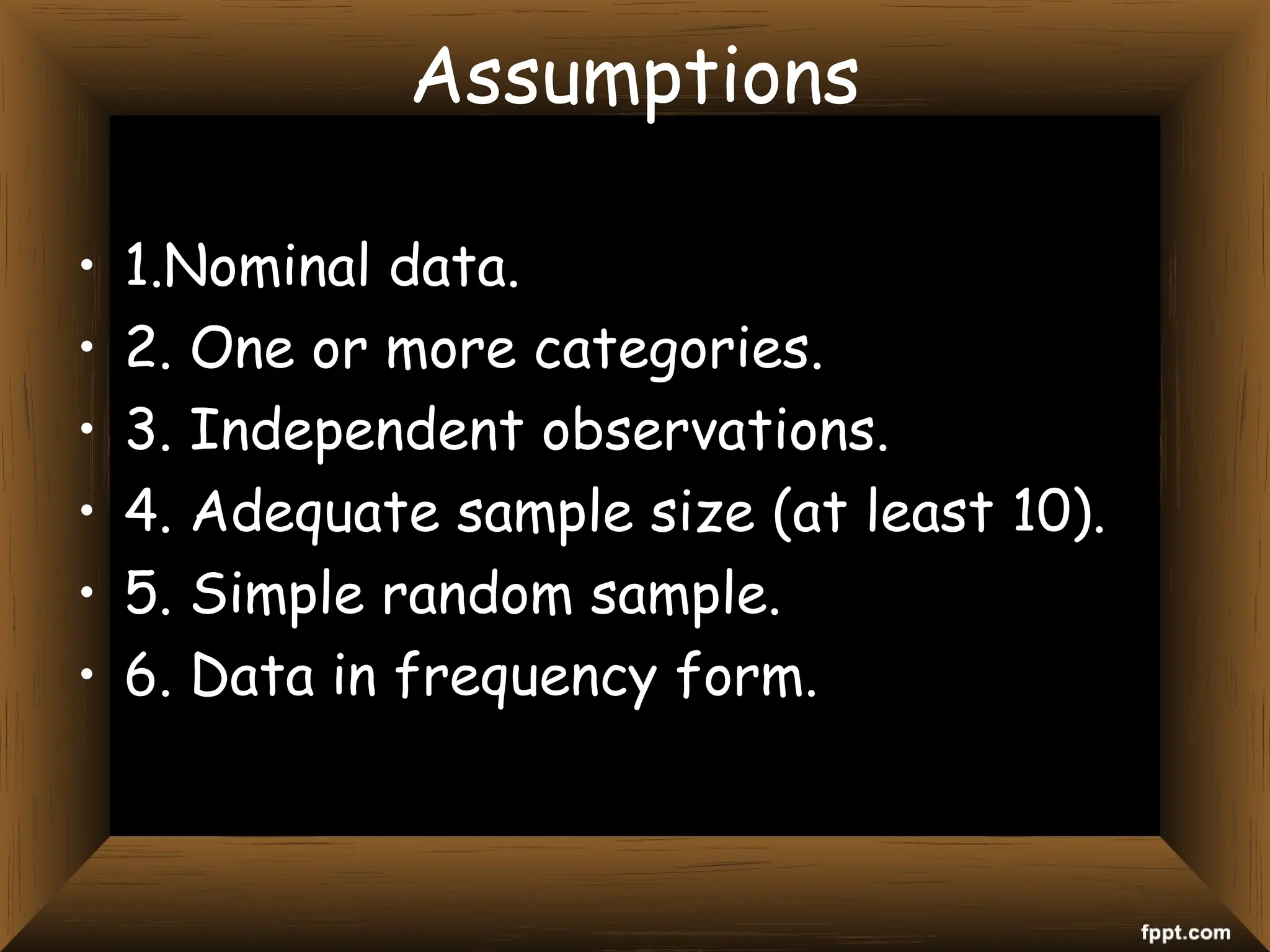
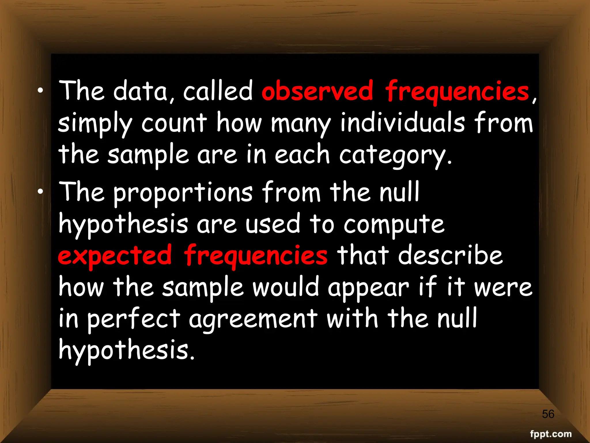
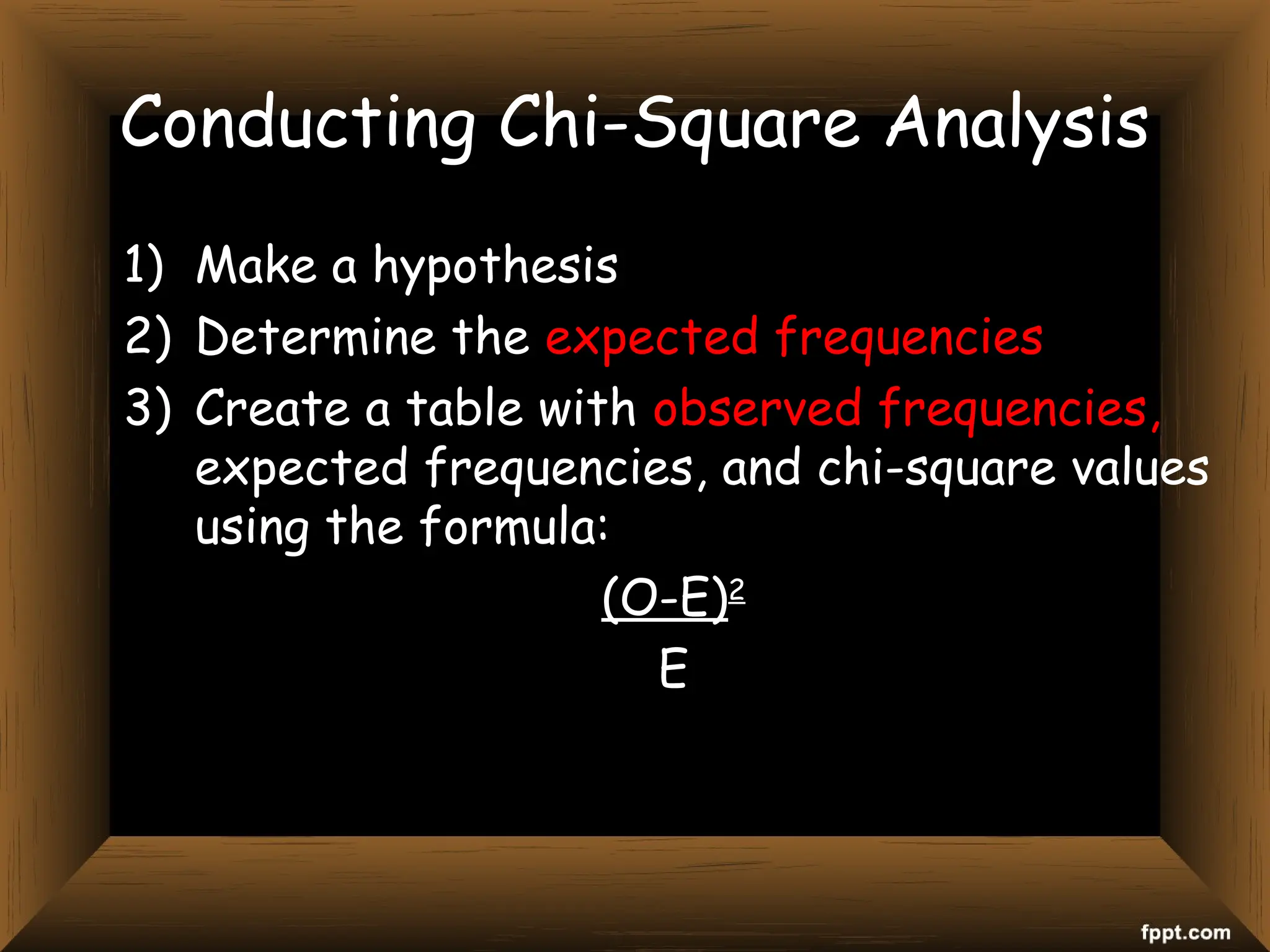
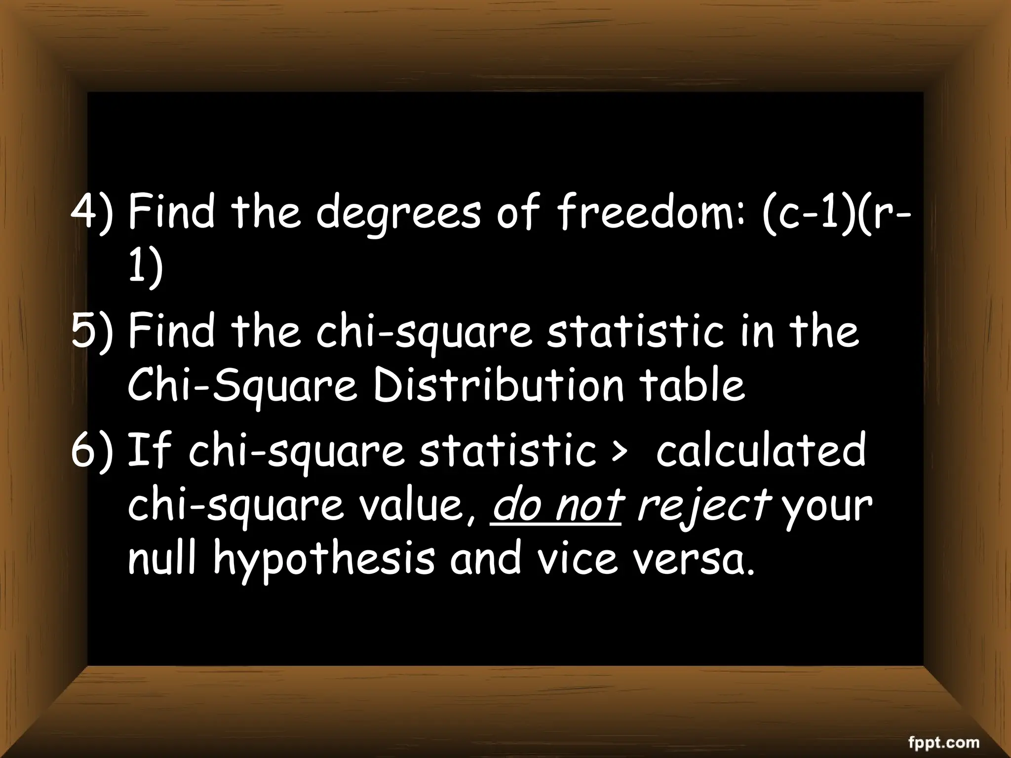
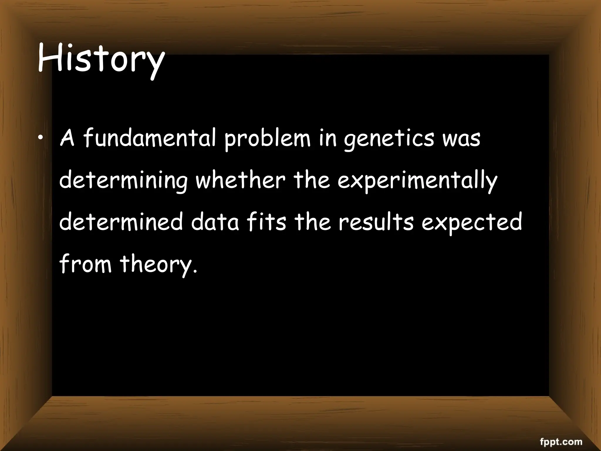
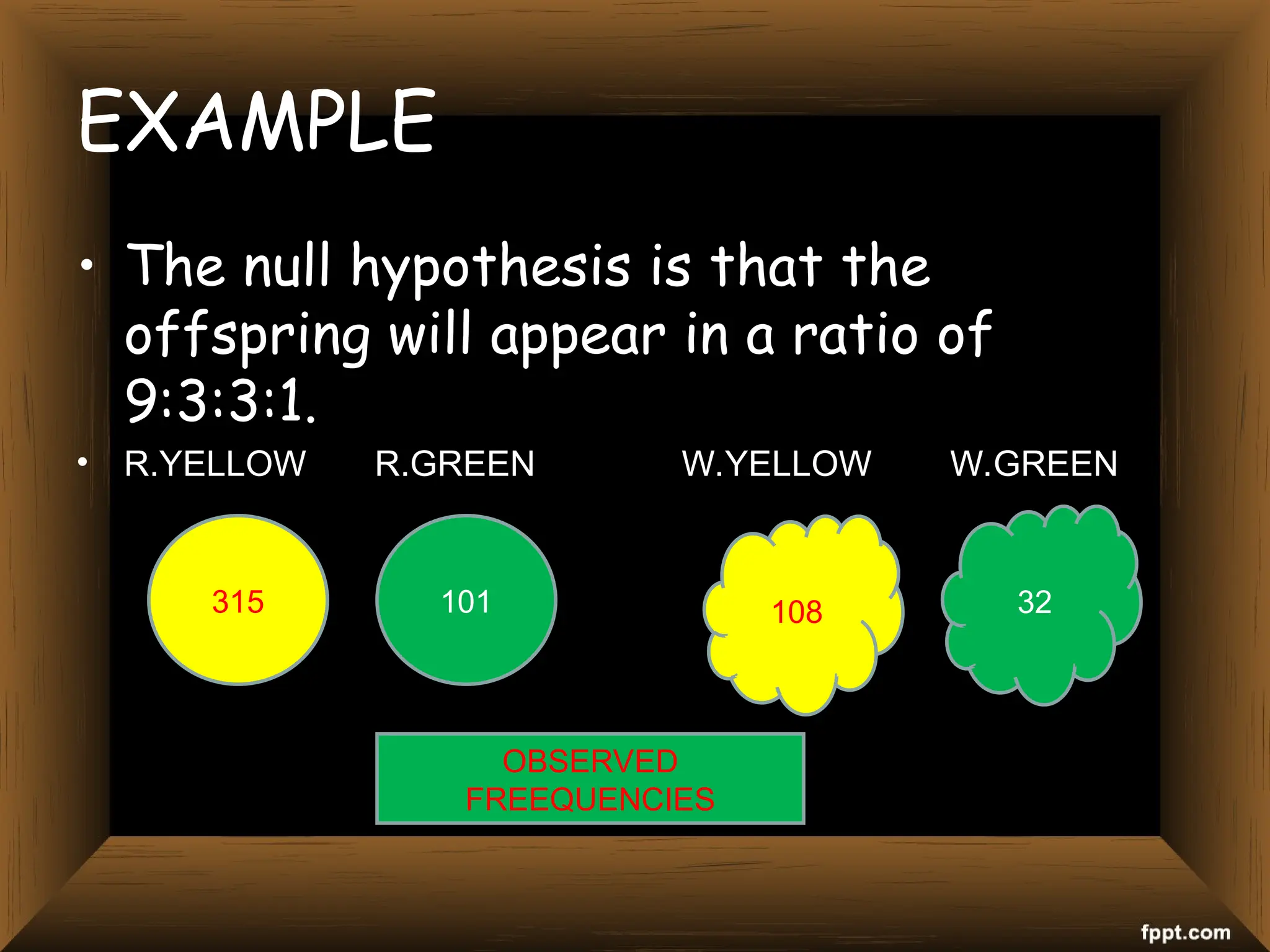
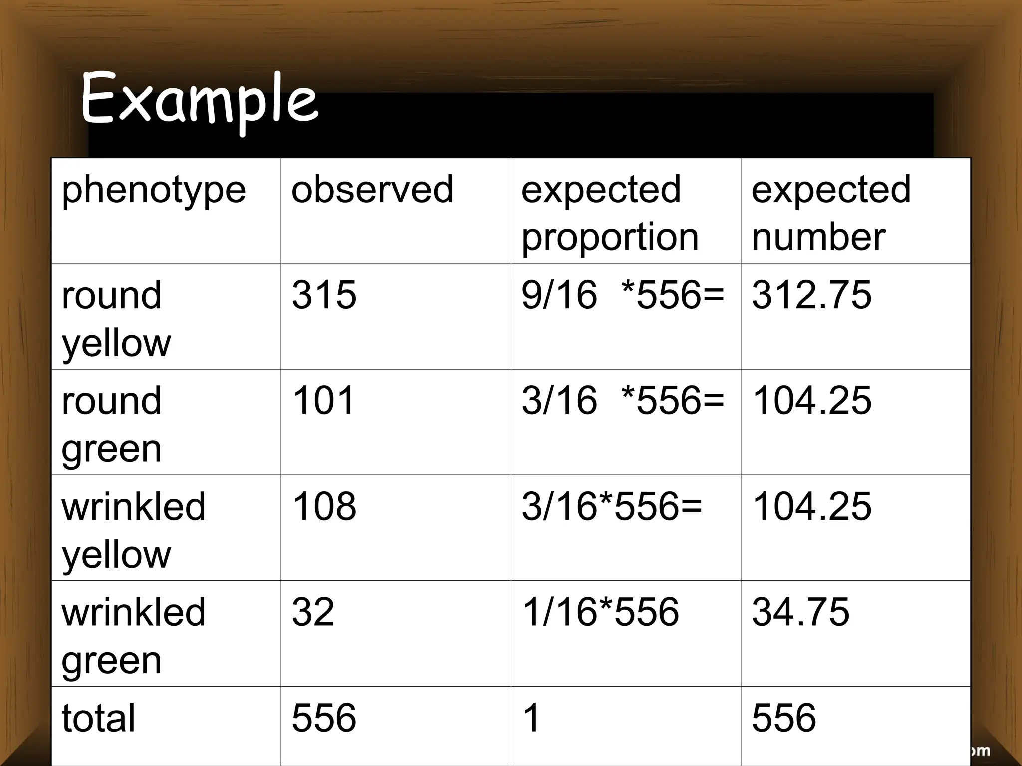
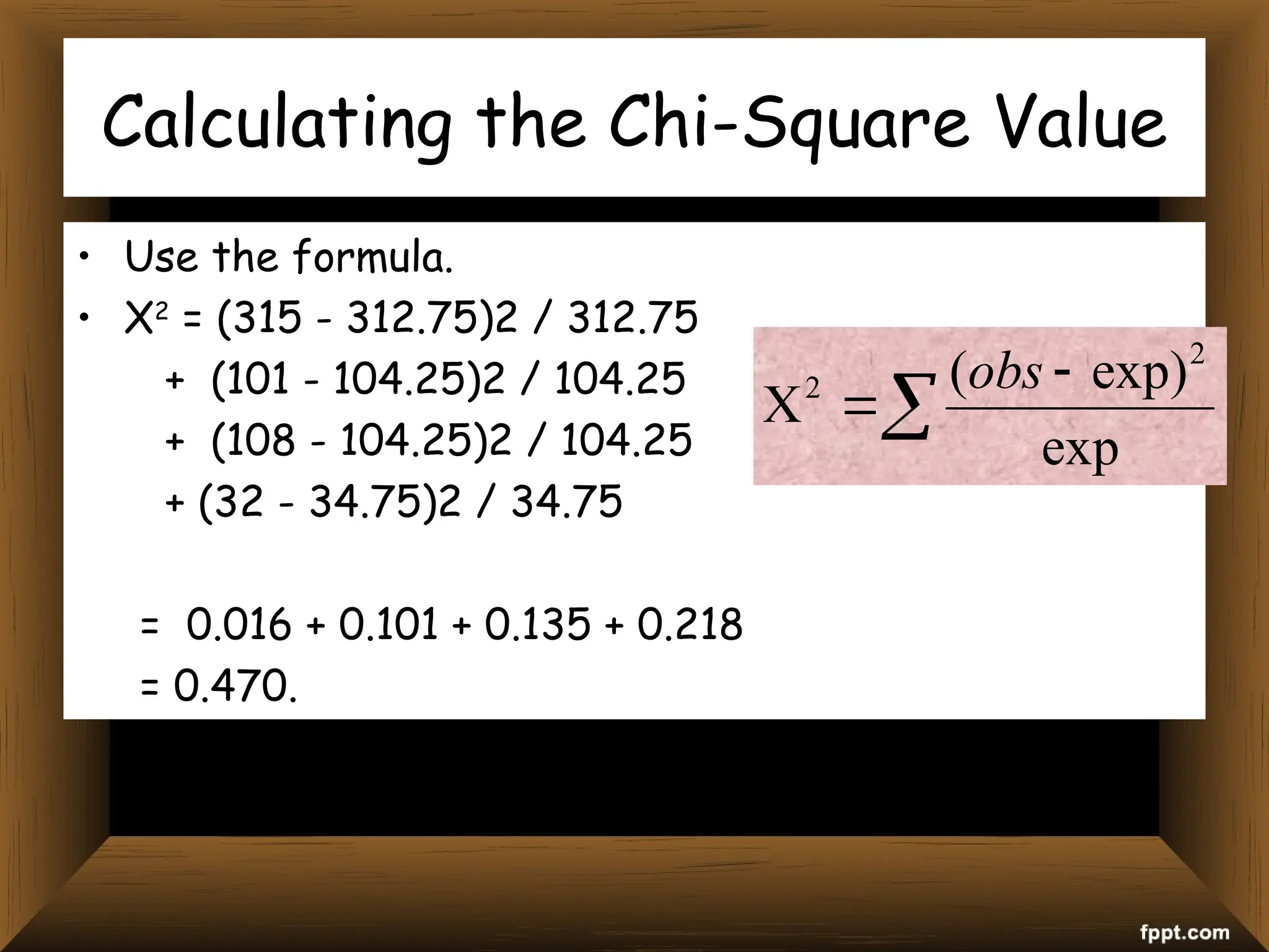
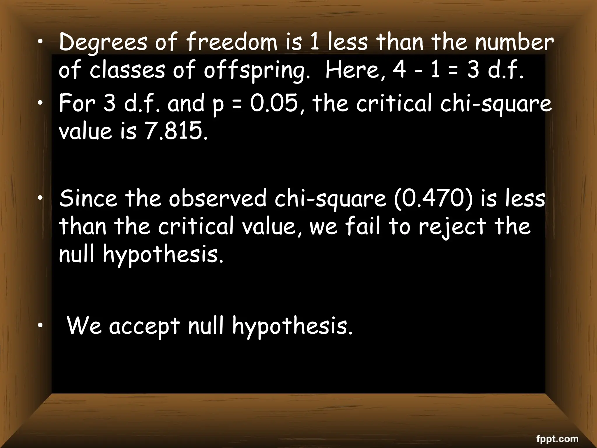
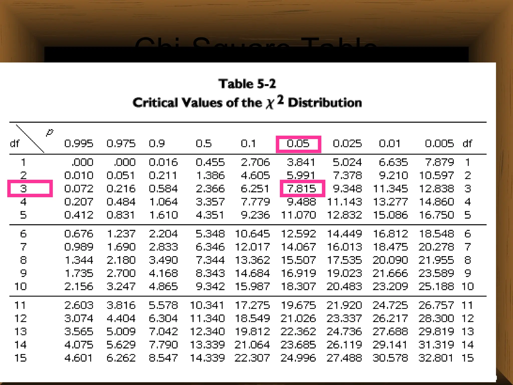
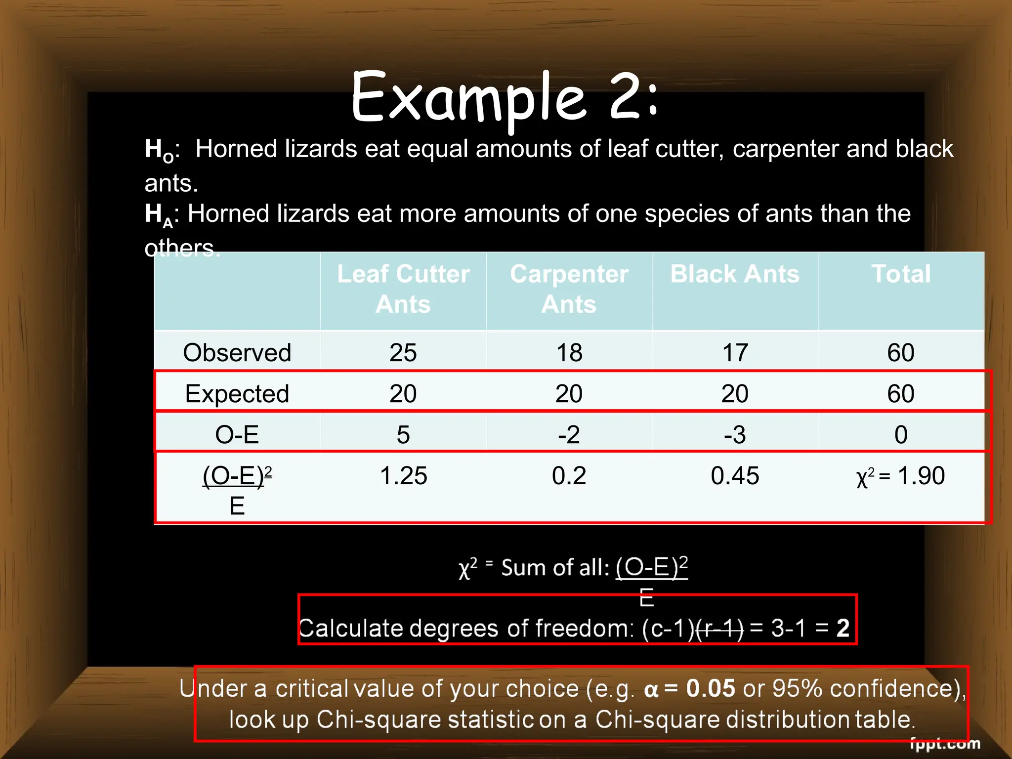
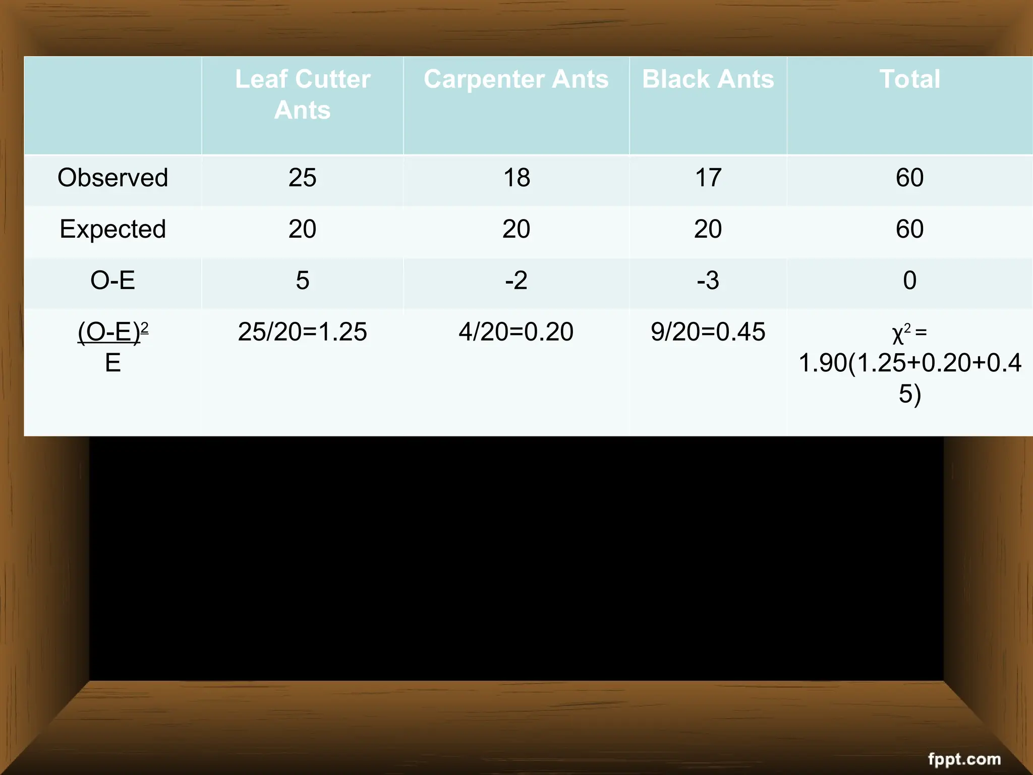
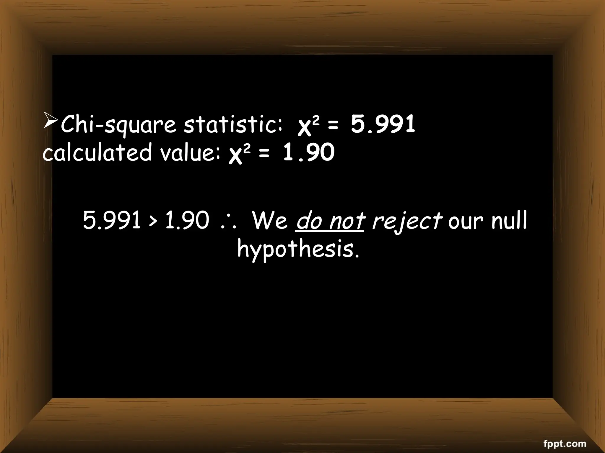
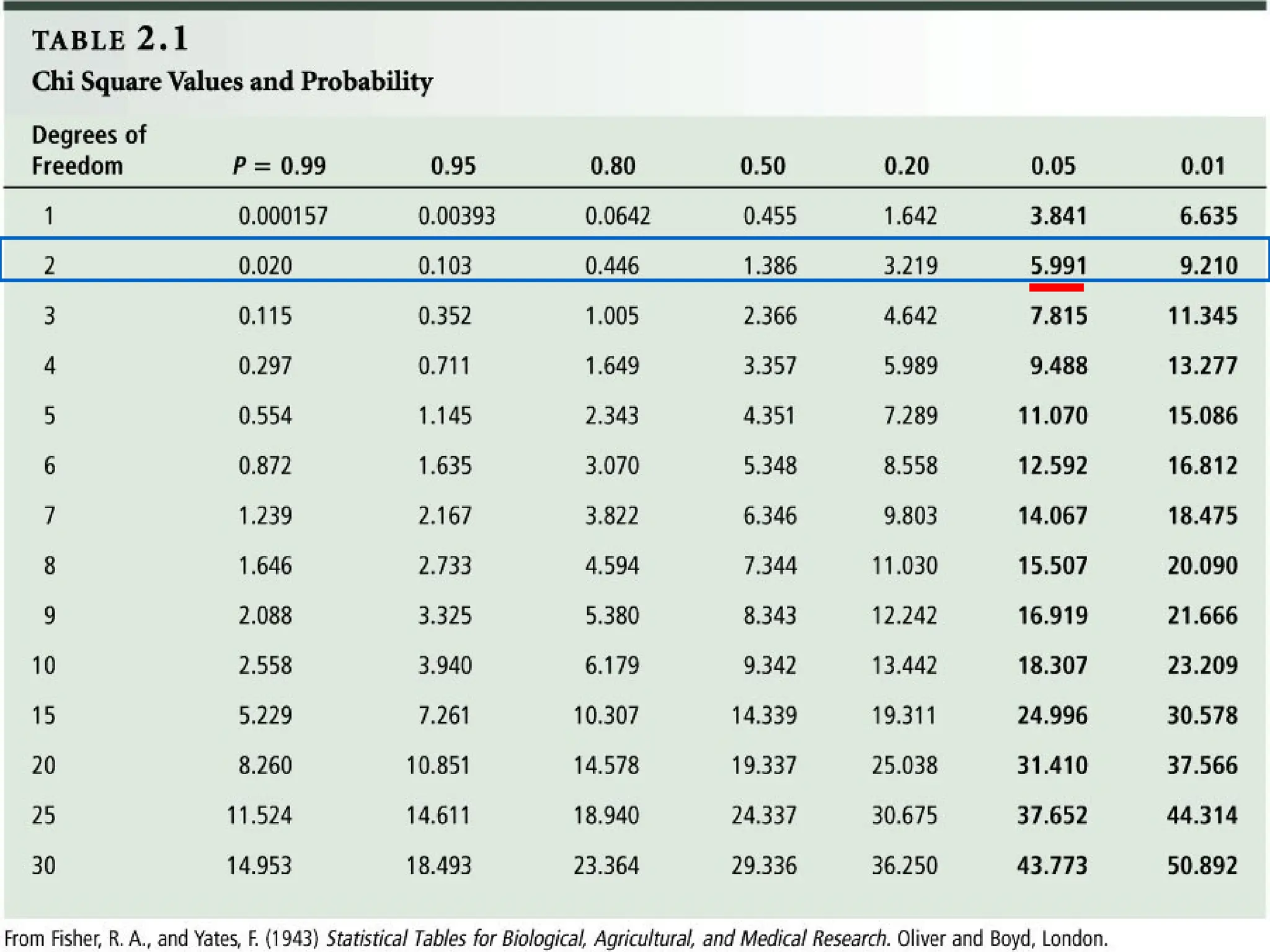
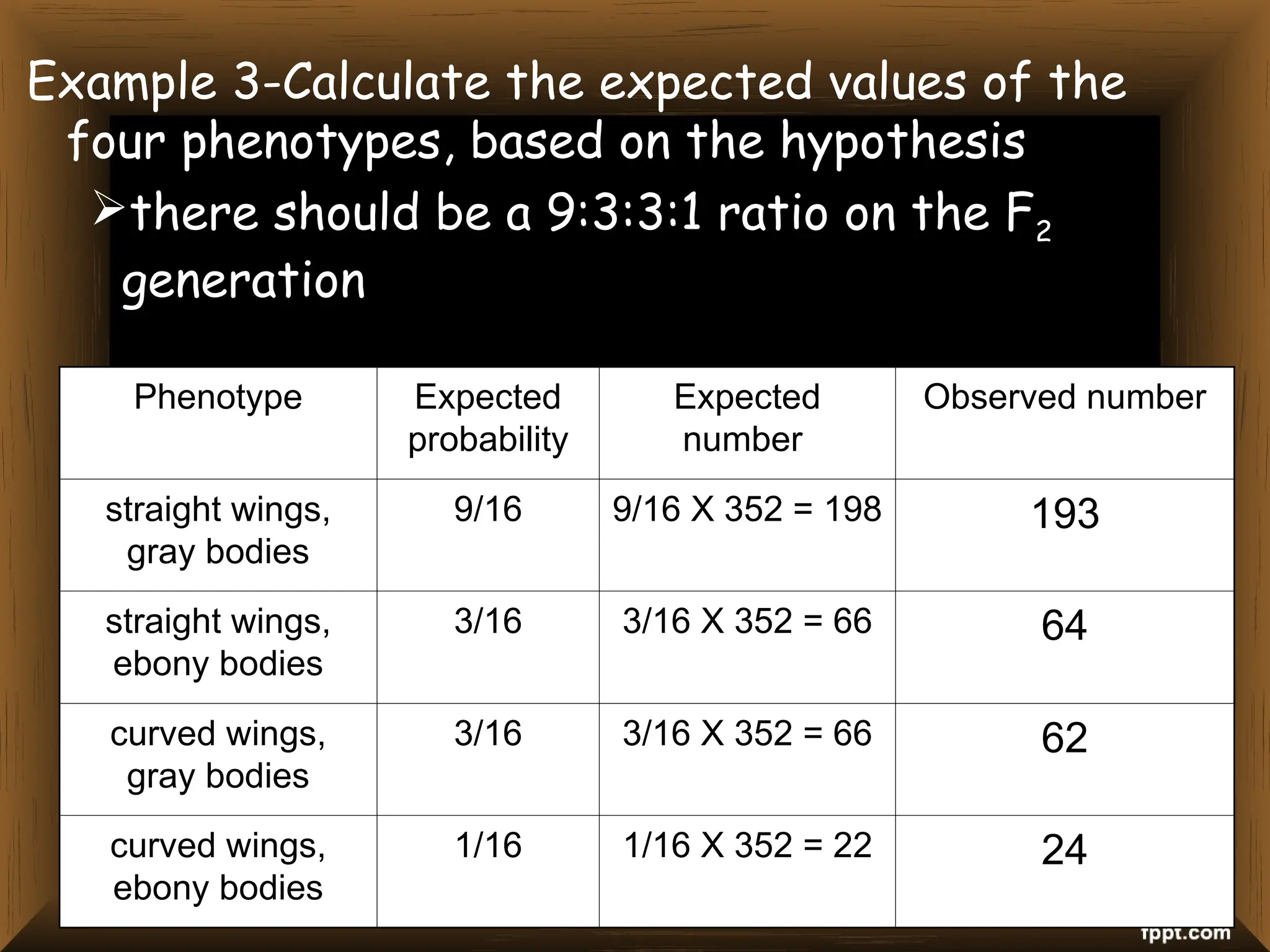
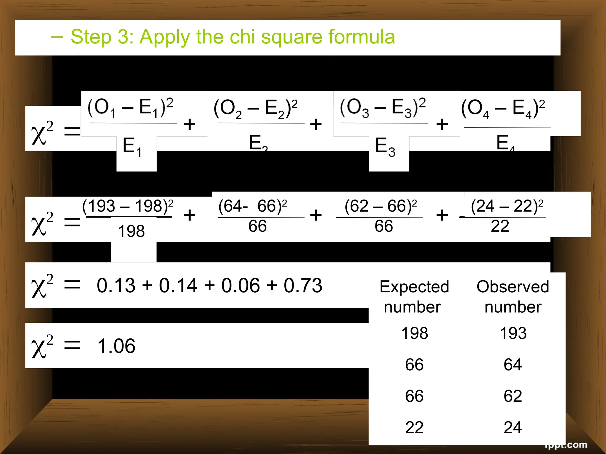
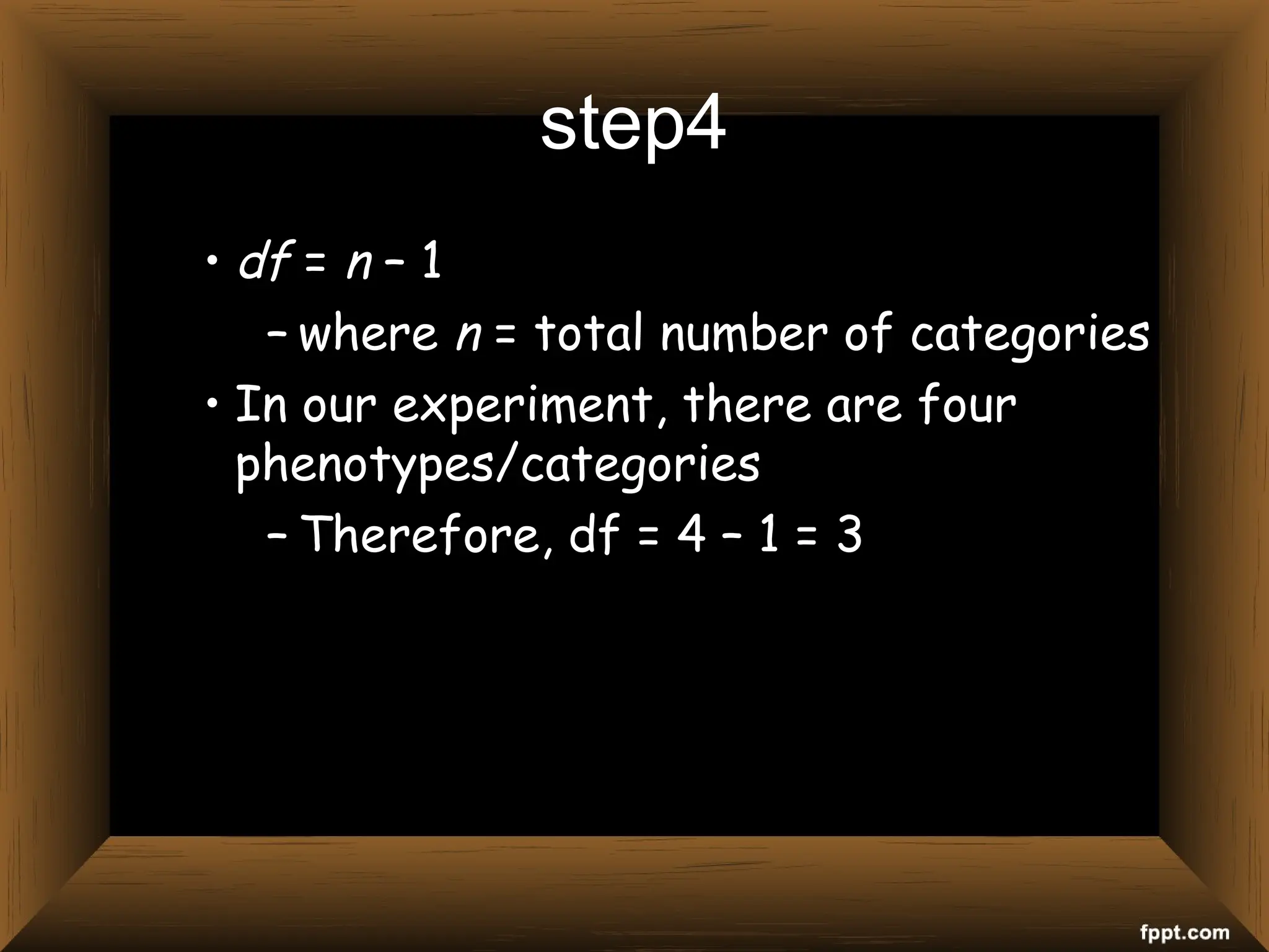
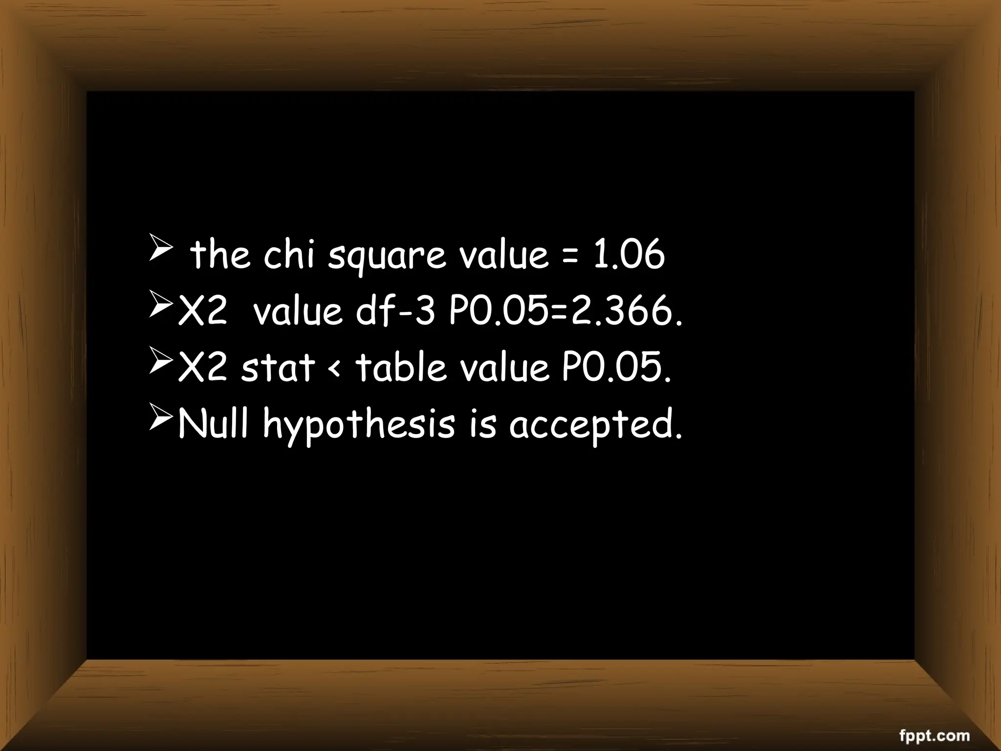
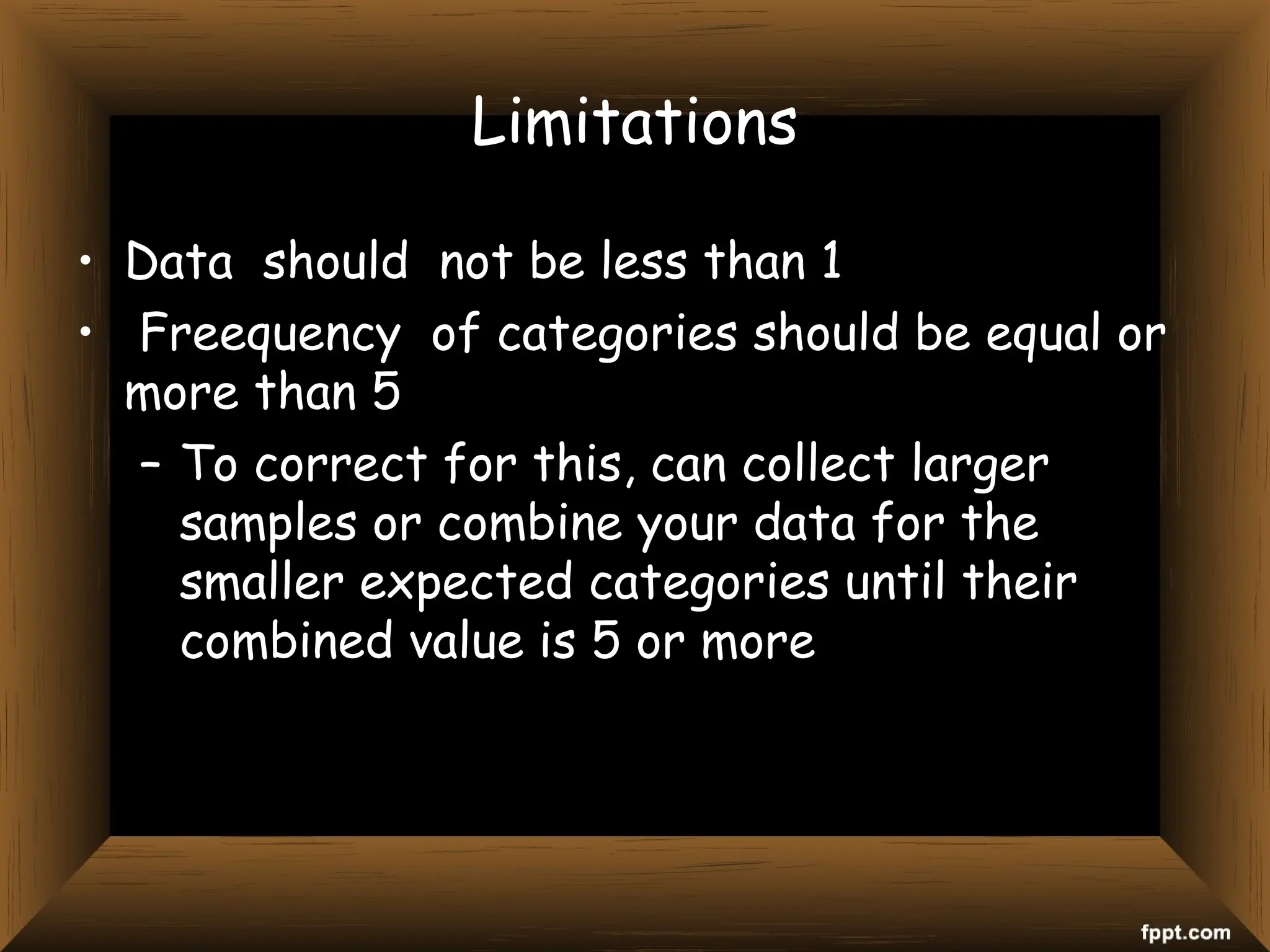
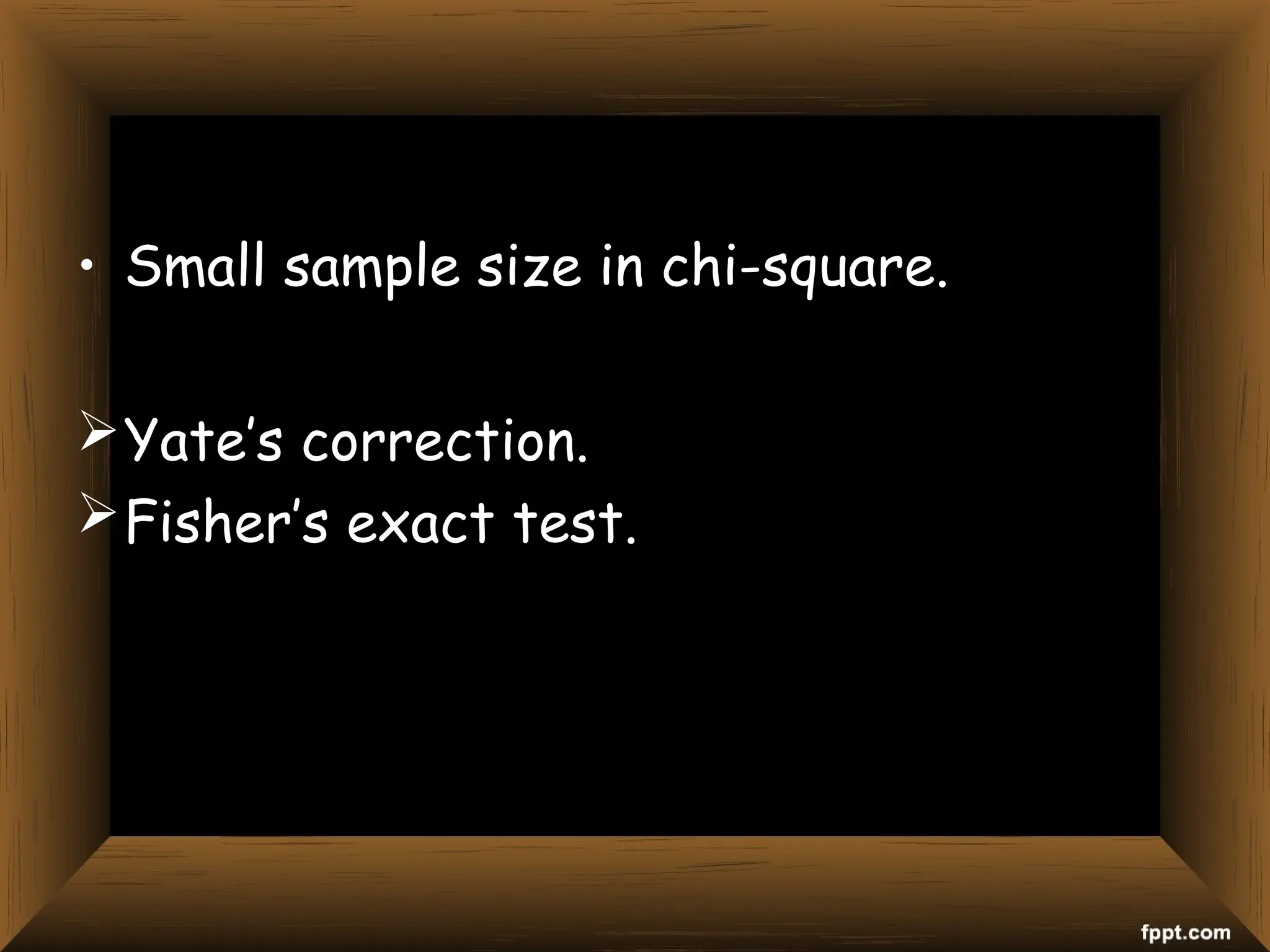
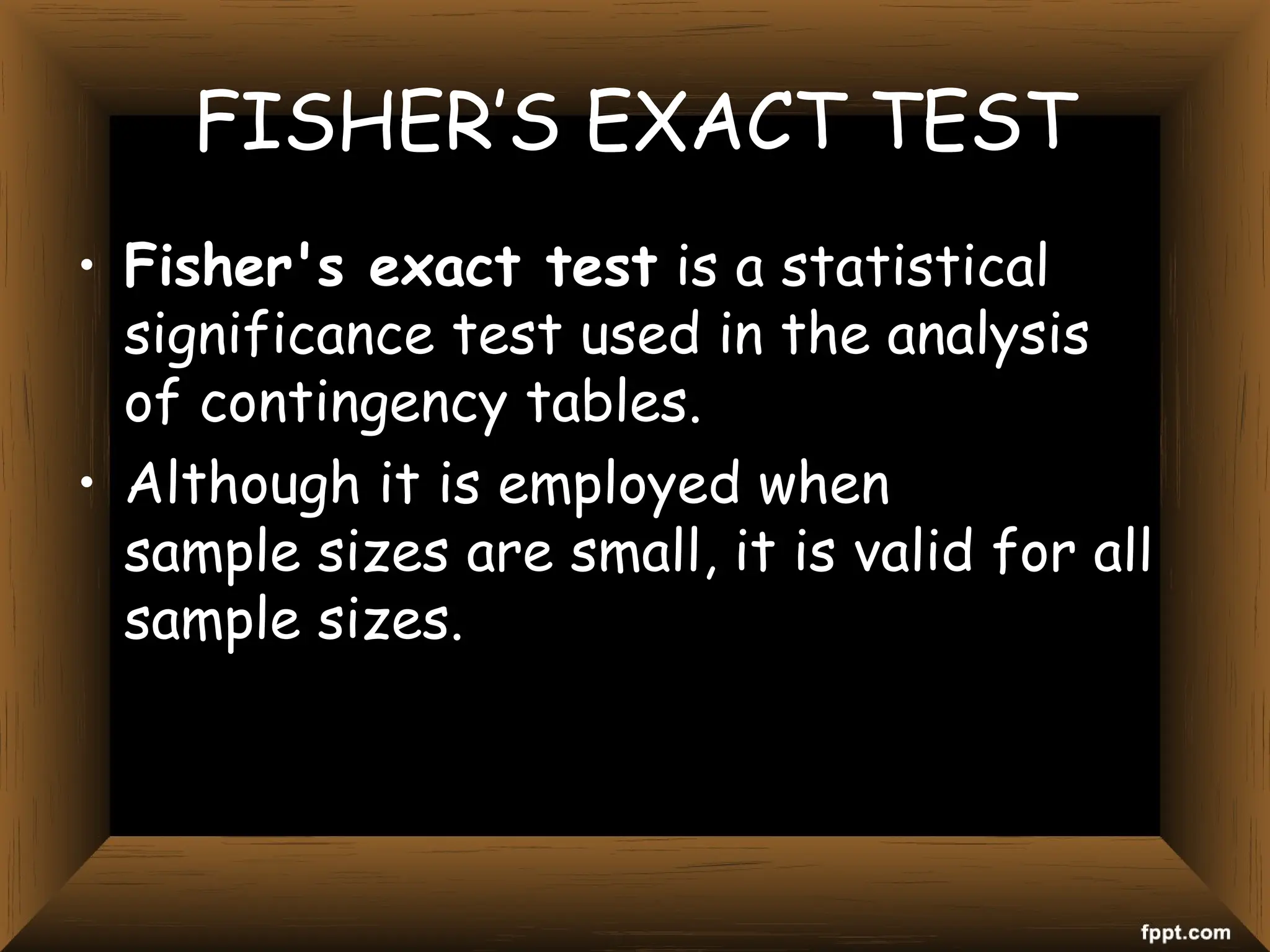
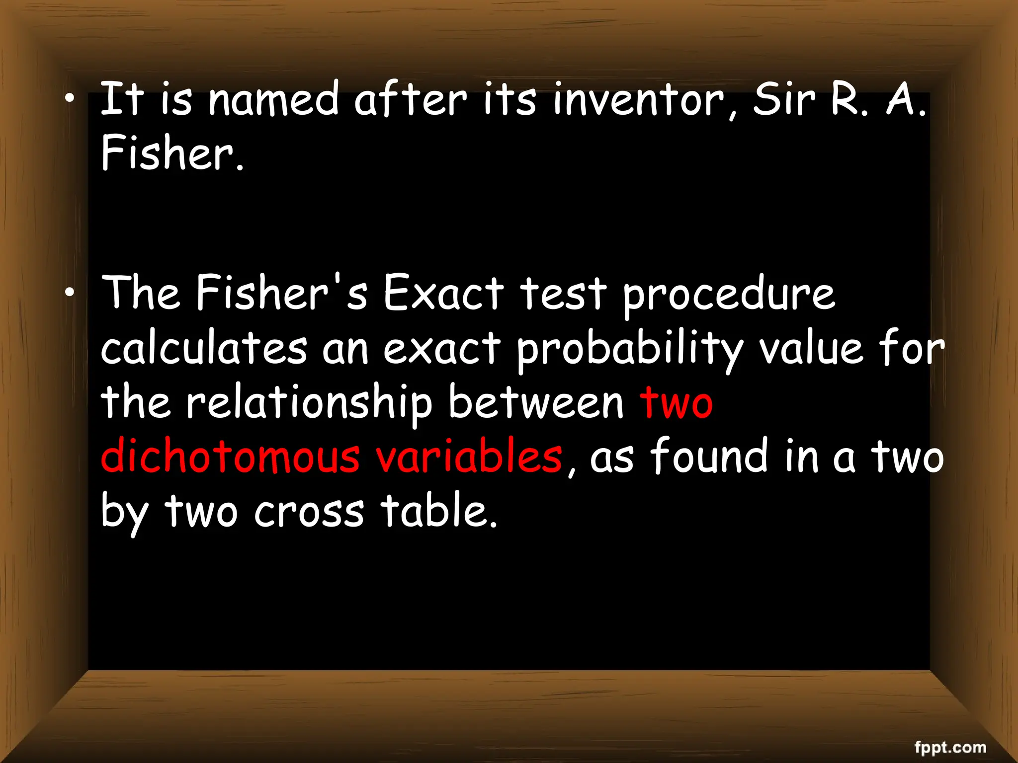
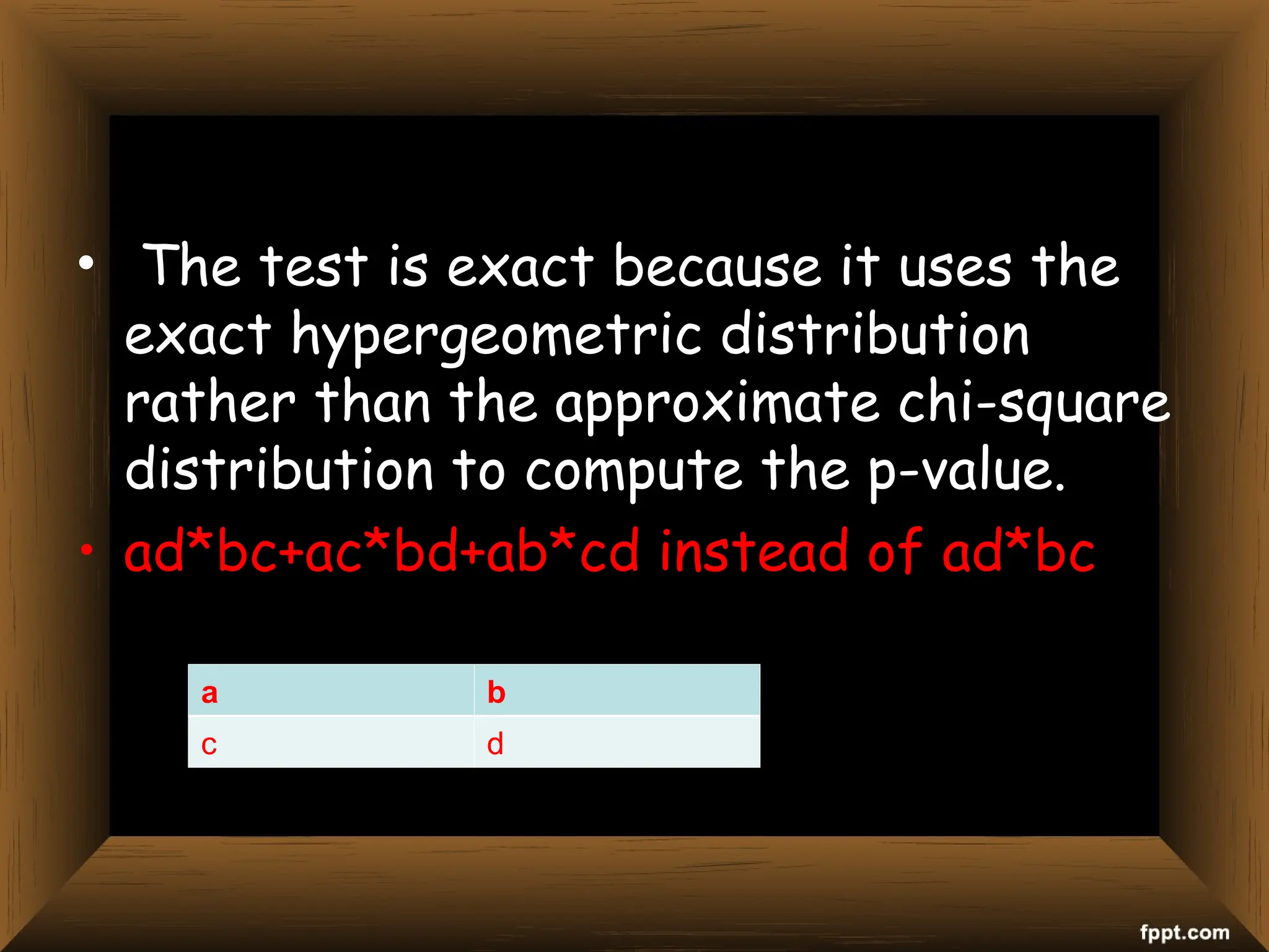
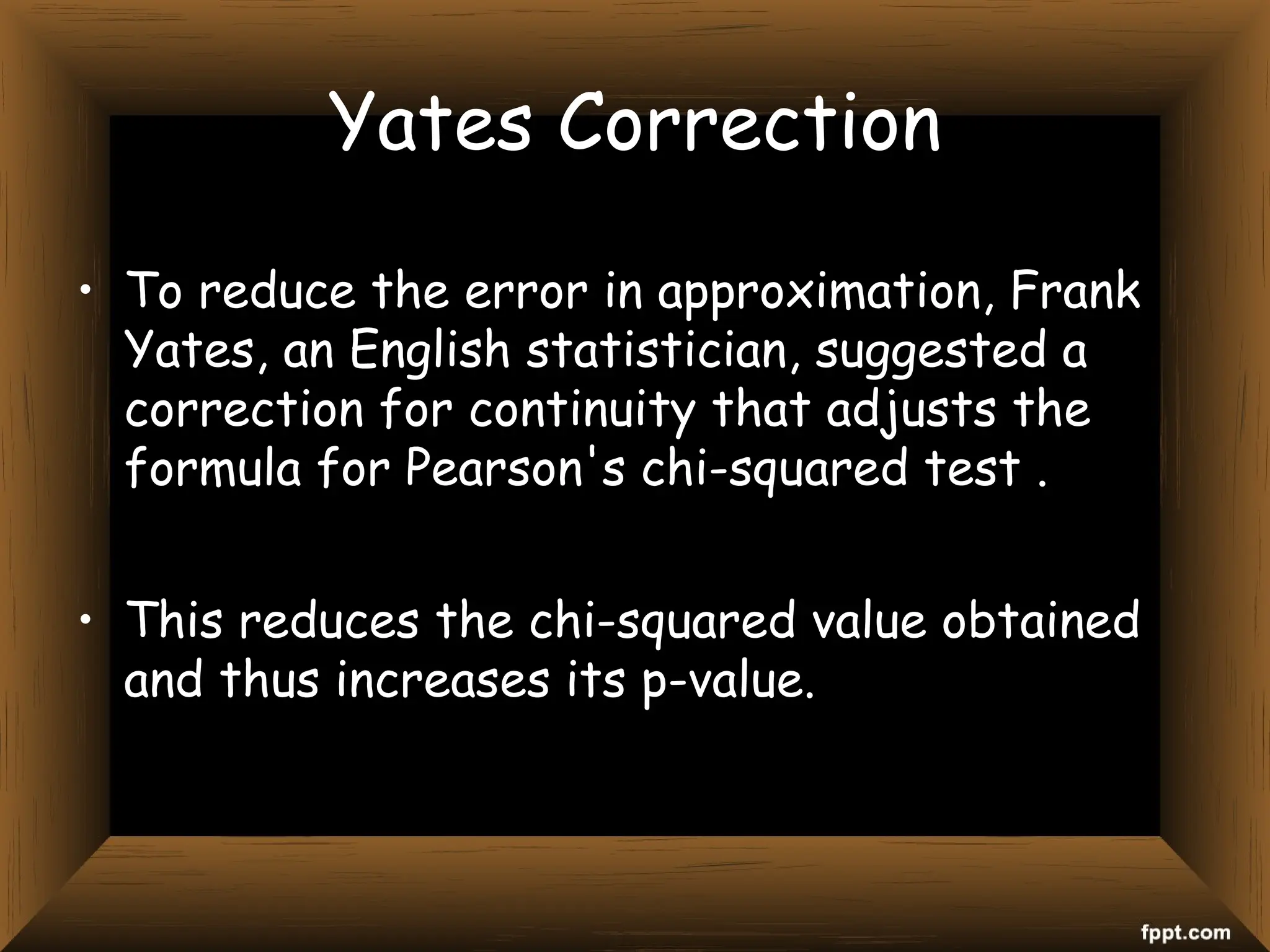
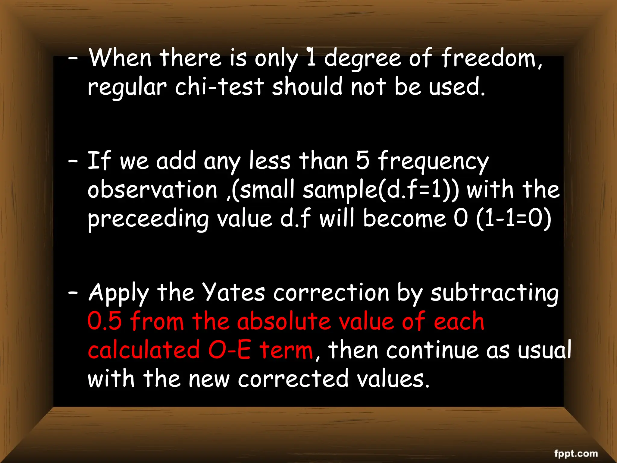
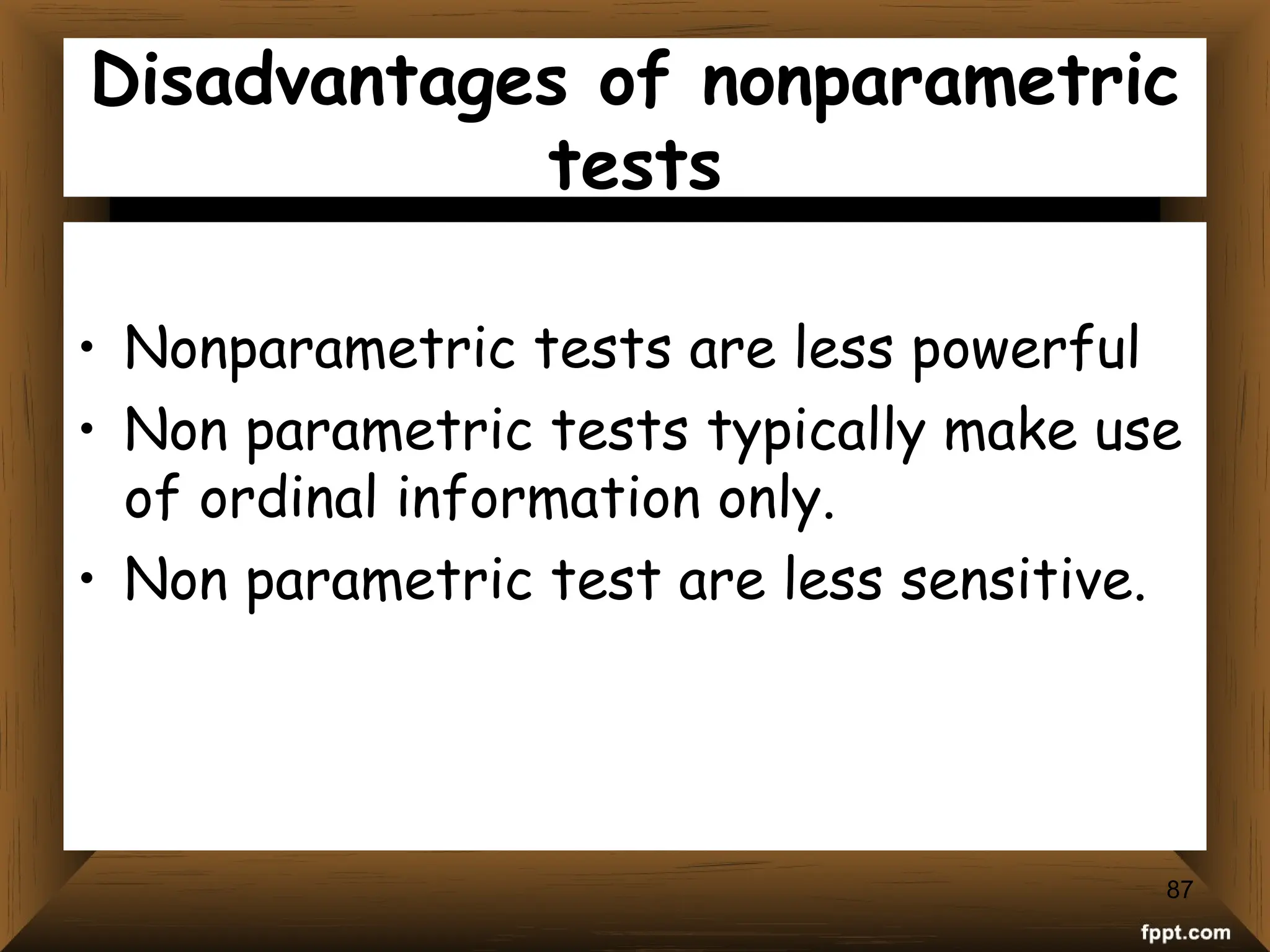
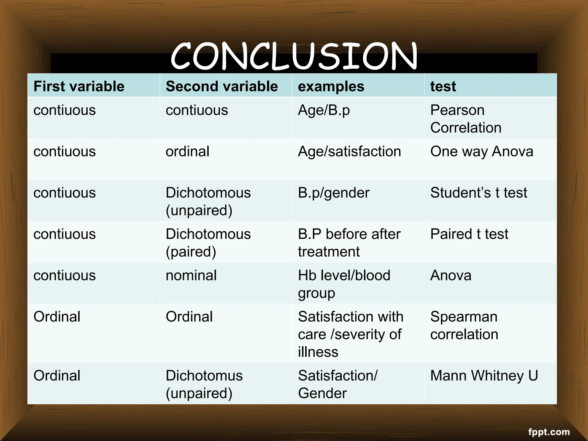
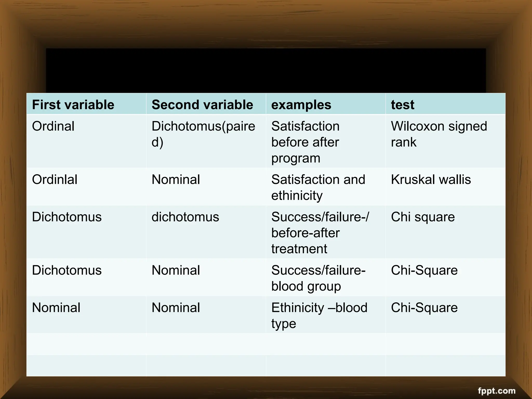
9-NON PARAMETRIC TEST in public health .ppt

Contents
• Introduction.
• Sign test.
• Wilcoxon Sign rank test-single sample.
• Wilcoxon sign rank test-paired sample.
• Wilcoxon Rank sum–Man Whitney U Test.
• Chi-Square test.
• Conclusion .
• References.

INTRODUCTION
Choice of Parametric or Non parametric
statistics depends on:
1/8/14 3

TYPE OF DATA
1. Nominal or Classificatory Scale
2. Ordinal or Ranking Scale
3. Interval Scale
4. Ratio Scale
Non
parametric
test
Parametric
test
4
1/8/14

Population
distribution
Symmetrical
distribution/
Normal
distribution
Asymmetric
distribution
Parametric
test
Non
Parametric
test
5
1/8/14

‘Parametric’ tests involve estimating
parameters such as the mean, and assume
that distribution of sample means are
‘normally’ distributed
• Often data does not follow a Normal
distribution.

skewed distribution
0 10 20 30 40 50
Units of alcohol per week
0
5
10
15
20
F
r
e
q
u
e
n
c
y
Mean = 8.03
Std. Dev. = 12.952
N = 30

• ‘Non-parametric’ tests were developed for
these situations where fewer assumptions
have to be made
• Non- parametric tests STILL have
assumptions but are less accurate.
• Non- parametric tests can be applied to
Normal data but parametric tests have
greater power .

Ranks
• Practical differences between parametric
and Non parametric tests are that Non
parametric methods use the ranks of values
rather than the actual values.
• E.g.
1,2,3,4,5,7,13,22,38,45 - actual
1,2,3,4,5,6, 7, 8, 9,10 - rank

EPI 809 / Spring 2008
Nonparametric Parametric
Sign Rank test One sample t-test
Wilcoxon Signed-Rank test paired sample t-test
Wilcoxon Rank – Sum test
(Mann-Whitney U test)
Two sample t-test
Chi-square

• One of the simplest of statistical test, it
focuses on the median rather than the mean
as a measure of central tendency.
• Only assumption made in performing the test
is that the variables come from a continuous
distribution.

• It is called the sign test because we use
pluses and minuses as the new data in
performing the calculations
• It is useful when we are not able to use
the t test because the assumption of
normality has been violated

• A sign test is used to decide whether a
binomial distribution has the equal
chance of observations above and below
median.
• It is a less powerful alternative to
the Wilcoxon signed rank test

• If the hypothesised median value were
true, we would expect:
• Approximately half of the sample values
to be larger than the hypothesised value
and the remaining half to be less than
it.

Disadvantage
• The sign test gives only directional
information .
• Magnitude information cannot be
obtained.

• H0=no difference in performance 0f device
1&2
• Test statstics is r stat = r min (r+,r-)
• r+=8 ,r-=4 so,r stat=4
• Table value at 0.05= 2
• r 0.05< r stat
• Reject null hypothesis.

• The test is named for Frank Wilcoxon (1892–
1965) who, in a single paper, proposed both
rank sign paired and the rank-sum test for
two independent samples .

• The test was popularized by Sidney
Siegel (1956) in his influential text book
“non-parametric statistics”. Siegel used
the symbol T .
• The test is sometimes referred to as
the Wilcoxon T test.

Assumptions
• Data are paired and from the same
population.
• Each pair/sample is chosen randomly
and independently.
• The data are measured on an ordinal
scale.need not be normal

Wicoxon test –one sample
• Observations
=280,282,292,273,283,283,283,275,28
4,282,279&281
• H0=population median=284
• Ha: population median <284

SL NO OBSERVATION OBSERVATION-
MEDIAN
ABSOLUTE
DIFFERENCE
RANK
1 280 -4 4 6
2 282 -2 2 3.5
3 292 8 8 8
4 273 -11 11 10
5 283 -1 1 1.5
6 283 -1 1 1.5
7 275 -9 9 9
8 284 0 0 -
9 282 -2 2 3.5
10 279 -5 5 7
11 281 -3 3 5

• W+=8
• W-=47
• W stat =wmin=8
• D.F=10(N-1 observation)
W (min) 8<W 0.05=11
So,we Accept null hypothesis.
Median=284

Example
The median heart rate for an 18 year old
girl is supposed to be 82bpm. A student
takes the pulse rates of 8 female
students (all aged 18):
83, 90, 96, 82, 85, 80, 81, 87
Do these results suggest that the median
might not be 82?

Wilcoxon Signed Rank Test:
Example
Result
Result Above or
Above or
below
below
median
median
Absolute
Absolute
difference from
difference from
median=82
median=82
Rank of
Rank of
difference
difference
83
83 +
+ 1
1 1.5
1.5
90
90 +
+ 8
8 6
6
96
96 +
+ 14
14 7
7
85
85 +
+ 3
3 4
4
80
80 -
- 2
2 3
3
81
81 -
- 1
1 1.5
1.5
87
87 +
+ 5
5 5
5

• W
W+
+= 1.5+6+7+4+5=23.5
= 1.5+6+7+4+5=23.5
• W
W-
-= 3+1.5=4.5
= 3+1.5=4.5 So, W=4.5
So, W=4.5
• D.f=6, so the value of W(4.5) > table
D.f=6, so the value of W(4.5) > table
value of 3
value of 3
• we reject null hypothesis
we reject null hypothesis

Wilcoxon paired Test
• To compare two related samples, matched
samples, or repeated measurements on a
single sample to assess whether their
population mean ranks differ.
• Equal to paired t test

Example
• An experiment is conducted to judge
the effect of brand name on quality
perception.
• 16 subjects are recruited for the
purpose and are asked to taste and
compare two samples of products

Wilcoxon test –paired sample
SL NO BRAND A BRAND B DIFFERENCE RANK
1 73 51 22 13
2 43 51 2 2.5
3 47 43 4 4.5
4 53 51 12 11
5 58 47 11 10
6 47 32 15 12
7 52 24 28 15
8 58 58 0 -
9 38 43 -5 6
10 61 53 8 8
11 56 52 4 4.5
12 56 57 -1 1
13 54 44 -10 9
14 55 57 -2 2.5
15 65 40 25 14
16 75 68 7 7

• W+=101.5
• W-=18.5
• D.f=15
• Significance level=0.05(Either W+ /W- less
than critical value ,reject null hypothesis)
• W test=W min =18.5
• Critic value=31>18.5
• Accept null hypothesis

• Wilcoxon Rank sum/ Man Whitney U
test

Assumption
• Ordinal data .
• Independent sample.
• Random observation.

HISTORY
• Henry Berthold Mann (1905- 2000, was
a professor
of mathematics and statistics at Ohio
State University.
• He and his student Whitney developed
the ("Mann-Whitney") U-
statistic of nonparametric statistics.

Example
• To compute the Mann
Whitney U:
– Rank the scores in both
groups (together) from
highest to lowest.
– Sum the ranks of the scores
for each group.
– The sum of ranks for each
group are used to make the
statistical comparison.
Income Rank NoIncome Rank
25 12 27 10
32 5 19 17
36 3 16 20
40 1 33 4
22 14 30 7
37 2 17 19
20 16 21 15
18 18 23 13
31 6 26 11
29 8 28 9
85 125

• The null hypothesis states that there is no
difference in income of 2 groups
• The Mann Whitney U statistic is

• U stat= smaller of U1 and U2.
• n1 = number of observations in group 1
• n2 = number of observations in group 2
• R1 = sum of the ranks assigned to group 1
• R2 = sum of the ranks assigned to group 2

• U1=n1*n2+(n1(n1+1)/2)-R1
= 10*10+(10(11)/2)-85
=100+(55)-85
=70
• U2=n1*n2+(n2(n2+1)/2)-R2
=100+55-125
=30
U MIN=30

• U at0.05(n10/10)= 27< 30(U test)
• Null hypothesis is rejected.

PEARSON’S CHI- SQUARED TEST
• Pearson's chi-squared test is used to
assess two types of comparison: tests
of goodness of fit and tests
of independence .

48
• The most obvious difference between
the chi square tests and the other
‑
hypothesis tests is the nature of the
data.
• For chi square, the data are
‑ frequencies
rather than numerical scores.

50
Goodness-of-Fit
• The chi-square test for goodness-of-fit
uses frequency data from a sample to test
hypotheses about the proportions of a
population.
• Each individual in the sample is classified into
one category on the scale of measurement.

• Goodness of fit establishes whether or
not an observed frequency
distribution differs from a theoretical
distribution.

Test Of Independence
• Assesses whether paired observations
on two variables, expressed in
a contingency table, are independent of
each other.

Contingency table
• In statistics, a contingency table (also
referred to as cross tabulation or cross tab)
is a type of table in a matrix format that
displays the (multivariate) frequency
distribution of the variables.
• 2 *2 table a b
c d

• The term contingency table was first used
by Karl Pearson in "On the Theory of
Contingency and Its Relation to Association
and Normal Correlation",

Assumptions
• 1.Nominal data.
• 2. One or more categories.
• 3. Independent observations.
• 4. Adequate sample size (at least 10).
• 5. Simple random sample.
• 6. Data in frequency form.

56
• The data, called observed frequencies,
simply count how many individuals from
the sample are in each category.
• The proportions from the null
hypothesis are used to compute
expected frequencies that describe
how the sample would appear if it were
in perfect agreement with the null
hypothesis.

Conducting Chi-Square Analysis
1) Make a hypothesis
2) Determine the expected frequencies
3) Create a table with observed frequencies,
expected frequencies, and chi-square values
using the formula:
(O-E)2
E

4) Find the degrees of freedom: (c-1)(r-
1)
5) Find the chi-square statistic in the
Chi-Square Distribution table
6) If chi-square statistic > calculated
chi-square value, do not reject your
null hypothesis and vice versa.

History
• A fundamental problem in genetics was
determining whether the experimentally
determined data fits the results expected
from theory.

• Mendel had no way of solving this problem.
Shortly after the discovery of his work in
1900, Karl Pearson and R.A. Fisher developed
the “chi-square” test for this purpose.

EXAMPLE
• The null hypothesis is that the
offspring will appear in a ratio of
9:3:3:1.
• R.YELLOW R.GREEN W.YELLOW W.GREEN
315 101 108 32
OBSERVED
FREEQUENCIES

Example
phenotype observed expected
proportion
expected
number
round
yellow
315 9/16 *556= 312.75
round
green
101 3/16 *556= 104.25
wrinkled
yellow
108 3/16*556= 104.25
wrinkled
green
32 1/16*556 34.75
total 556 1 556

Calculating the Chi-Square Value
• Use the formula.
• X2
= (315 - 312.75)2 / 312.75
+ (101 - 104.25)2 / 104.25
+ (108 - 104.25)2 / 104.25
+ (32 - 34.75)2 / 34.75
= 0.016 + 0.101 + 0.135 + 0.218
= 0.470.




exp
exp)
( 2
2 obs

• Degrees of freedom is 1 less than the number
of classes of offspring. Here, 4 - 1 = 3 d.f.
• For 3 d.f. and p = 0.05, the critical chi-square
value is 7.815.
• Since the observed chi-square (0.470) is less
than the critical value, we fail to reject the
null hypothesis.
• We accept null hypothesis.

Example 2:
Leaf Cutter
Ants
Carpenter
Ants
Black Ants Total
Observed 25 18 17 60
Expected 20 20 20 60
O-E 5 -2 -3 0
(O-E)2
E
1.25 0.2 0.45 χ2
= 1.90
HO: Horned lizards eat equal amounts of leaf cutter, carpenter and black
ants.
HA: Horned lizards eat more amounts of one species of ants than the
others.

Leaf Cutter
Ants
Carpenter Ants Black Ants Total
Observed 25 18 17 60
Expected 20 20 20 60
O-E 5 -2 -3 0
(O-E)2
E
25/20=1.25 4/20=0.20 9/20=0.45 χ2
=
1.90(1.25+0.20+0.4
5)

Chi-square statistic: χ2
= 5.991
calculated value: χ2
= 1.90
5.991 > 1.90 ∴ We do not reject our null
hypothesis.

Example 3-Calculate the expected values of the
four phenotypes, based on the hypothesis
there should be a 9:3:3:1 ratio on the F2
generation
Phenotype Expected
probability
Expected
number
Observed number
straight wings,
gray bodies
9/16 9/16 X 352 = 198 193
straight wings,
ebony bodies
3/16 3/16 X 352 = 66 64
curved wings,
gray bodies
3/16 3/16 X 352 = 66 62
curved wings,
ebony bodies
1/16 1/16 X 352 = 22 24

– Step 3: Apply the chi square formula



(O2 – E2)2
E2

(O4 – E4)2
E4

+ + +



(193 – 198)2
198

(64- 66)2
66

(62 – 66)2
66

(24 – 22)2
22

+ + +

0.13 + 0.14 + 0.06 + 0.73

1.06
Expected
number
Observed
number
198 193
66 64
66 62
22 24

step4
• df = n – 1
– where n = total number of categories
• In our experiment, there are four
phenotypes/categories
– Therefore, df = 4 – 1 = 3

 the chi square value = 1.06
X2 value df-3 P0.05=2.366.
X2 stat < table value P0.05.
Null hypothesis is accepted.

Limitations
• Data should not be less than 1
• Freequency of categories should be equal or
more than 5
– To correct for this, can collect larger
samples or combine your data for the
smaller expected categories until their
combined value is 5 or more

• Small sample size in chi-square.
Yate’s correction.
Fisher’s exact test.

FISHER’S EXACT TEST
• Fisher's exact test is a statistical
significance test used in the analysis
of contingency tables.
• Although it is employed when
sample sizes are small, it is valid for all
sample sizes.

• It is named after its inventor, Sir R. A.
Fisher.
• The Fisher's Exact test procedure
calculates an exact probability value for
the relationship between two
dichotomous variables, as found in a two
by two cross table.

• The test is exact because it uses the
exact hypergeometric distribution
rather than the approximate chi-square
distribution to compute the p-value.
• ad*bc+ac*bd+ab*cd instead of ad*bc
a b
c d

• So we get exact p value which will be
more likely to be significant than chi-
square value..

Yates Correction
• To reduce the error in approximation, Frank
Yates, an English statistician, suggested a
correction for continuity that adjusts the
formula for Pearson's chi-squared test .
• This reduces the chi-squared value obtained
and thus increases its p-value.

.
– When there is only 1 degree of freedom,
regular chi-test should not be used.
– If we add any less than 5 frequency
observation ,(small sample(d.f=1)) with the
preceeding value d.f will become 0 (1-1=0)
– Apply the Yates correction by subtracting
0.5 from the absolute value of each
calculated O-E term, then continue as usual
with the new corrected values.

Advantages of non parametric
tests
• Advantages of nonparametric tests
1 These test can be used if the sample
size is very small and distribution of
population is not known exactly.
2. Nonparametric tests typically make
fewer assumptions about the data.
83

3. Nonparametric tests are available to analyze
data which are at ordinal scale. (in ranks)
• For example, in studying a variable such as
anxiety, we may be able to state that subject A
is more anxious than subject B without knowing
at all exactly how much more anxious A is.
• If data are inherently in ranks they can be
treated by nonparametric methods, whereas they
cannot be treated by parametric methods.
84

4. Because these tests deals with rank rather
than actual observed value non parametric
tests are less sensitive to measurement
errors.
5. Nonparametric methods are available to treat
data which are simply classificatory or
categorical, i.e., are measured in a nominal
scale.
85

6. Nonparametric statistical tests are typically
much easier to learn and to apply.
7. These tests are easier to understand and less
computation is required.
86

Disadvantages of nonparametric
tests
• Nonparametric tests are less powerful
• Non parametric tests typically make use
of ordinal information only.
• Non parametric test are less sensitive.
87

CONCLUSION
First variable Second variable examples test
contiuous contiuous Age/B.p Pearson
Correlation
contiuous ordinal Age/satisfaction One way Anova
contiuous Dichotomous
(unpaired)
B.p/gender Student’s t test
contiuous Dichotomous
(paired)
B.P before after
treatment
Paired t test
contiuous nominal Hb level/blood
group
Anova
Ordinal Ordinal Satisfaction with
care /severity of
illness
Spearman
correlation
Ordinal Dichotomus
(unpaired)
Satisfaction/
Gender
Mann Whitney U

First variable Second variable examples test
Ordinal Dichotomus(paire
d)
Satisfaction
before after
program
Wilcoxon signed
rank
Ordinlal Nominal Satisfaction and
ethinicity
Kruskal wallis
Dichotomus dichotomus Success/failure-/
before-after
treatment
Chi square
Dichotomus Nominal Success/failure-
blood group
Chi-Square
Nominal Nominal Ethinicity –blood
type
Chi-Square

References
1. Kothari CR . Research methodology: methods
and techniques. 3rd
ed.. p. 147-206
2. Jekel J.F., Katz D.L., Elmore J.G. and Wild
D.M.G. Epidemiology, Biostatistics and
Preventive Medicine. 3rd
ed .p139-174
3. Mahajan. Methods in biostatistics. 200 .7th
ed. 70-9, 93-157
90
1/8/14

4.Rao KV:Biostatistics: A manual of statistical
methods for use in health, nutrition and
anthropology.,. 2nd
ed, p.51-90,131-98
5. Rao.S P.S.S and Richard J. An Introduction
To Biostatistics and research methods. 4th
edition :p 55-57,66-83
6.GN Prabhakara:Biostastics;1st
edition;p 74-
102,162-172
91
1/8/14

• 7. Donald Ary, Lucy Chese Jacobs & Asghar
Razavieh, Introduction to Research in
Education: Holt, Rinehart and Winston, Inc.,
1984.

9-NON PARAMETRIC TEST in public health .ppt

More Related Content

Similar to 9-NON PARAMETRIC TEST in public health .ppt

Recently uploaded

9-NON PARAMETRIC TEST in public health .ppt

Editor's Notes