Principal Component Analysis (PCA) and LDA PPT Slides

Principal Component Analysis (PCA) and LDA PPT Slides

• 1.
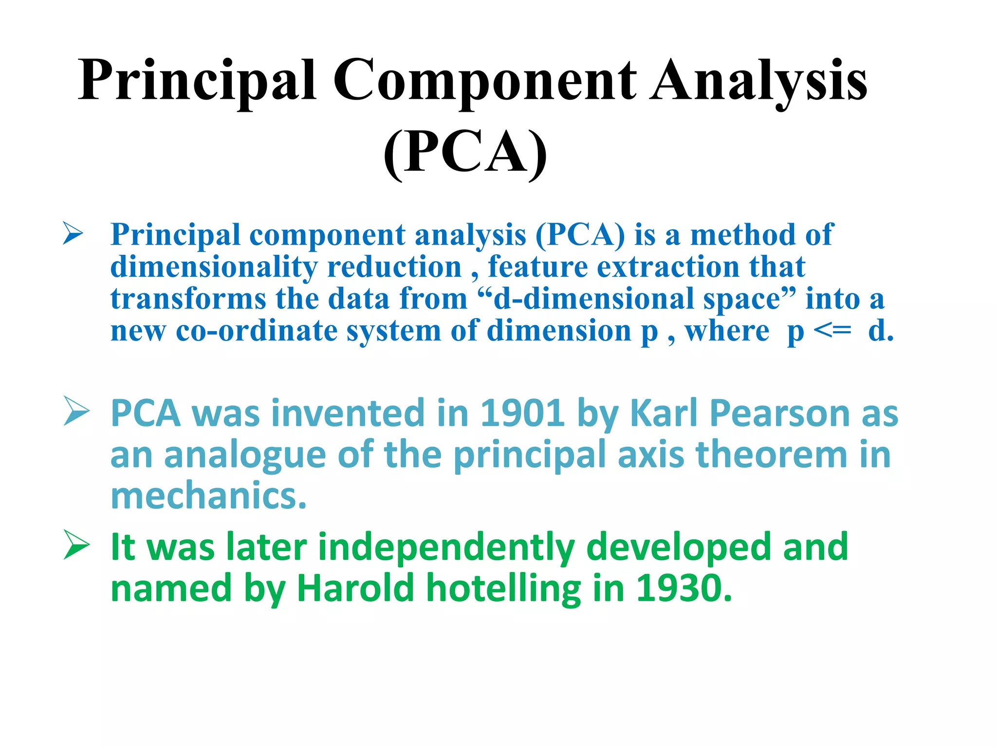
  Principal Component Analysis (PCA) Principal component analysis (PCA) is a method of dimensionality reduction , feature extraction that transforms the data from “d-dimensional space” into a new co-ordinate system of dimension p , where p <= d.  PCA was invented in 1901 by Karl Pearson as an analogue of the principal axis theorem in mechanics.  It was later independently developed and named by Harold hotelling in 1930.
• 2.
  Goals The main goalof a PCA analysis is to identify patterns in data. It is basically used to reduce the dimensions of data set .  PCA aims to detect the correlation between variables.
• 3.
  Transformation  In orderto approximate the space spanned by the original data points. X=[x1,x2x3,……….,xd] we can chose p based on what percentage of the variance of the original data we would lie to maintain .  The first principal component has the maximum variance , thus it accounts for the most significant variance in data.  The Second principal component has the second highest variance and so on until principal component has minimum variance
• 4.
  PCA Approach Standardize thedata. Perform Singular Vector Decomposition to get the Eigenvectors and Eigenvalues. Sort eigenvalues in descending order and choose the k- eigenvectors Construct the projection matrix from the selected k- eigenvectors. Transform the original dataset via projection matrix to obtain a k-dimensional feature subspace.
• 5.
  After PCA
• 6.
  Different types ofPCA Scatter plots for better understanding
• 7.
  Linear Discriminant Analysis (LDA)
• 8.
  Introduction Linear Discriminant Analysis(LDA) is used to solve dimensionality reduction for data with higher attributes  Pre-processing step for pattern-classification and machine learning applications.  Used for feature extraction.  Linear transformation that maximize the separation between multiple classes.  The original dichotomous discriminant analysis was developed by Sir Ronald Fisher in 1936.
• 9.
  Feature Subspace : Toreduce the dimensions of a d-dimensional data set by projecting it onto a (k)-dimensional subspace (where k < d) Feature space data is well represented:- Compute eigen vectors from dataset Collect them in scatter matrix Generate k-dimensional data from d-dimensional dataset.
• 10.
  Scatter Matrix: Within classscatter matrix In between class scatter matrix Maximize the between class measure & minimize the within class measure.
• 11.
  LDA steps: 1. Computethe d-dimensional mean vectors. 2. Compute the scatter matrices 3. Compute the eigenvectors and corresponding eigenvalues for the scatter matrices. 4. Sort the eigenvalues and choose those with the largest eigenvalues to form a d×k dimensional matrix 5. Transform the samples onto the new subspace.
• 13.
  Different types ofLDA Scatter plots for better understanding
• 14.
  References: [1]https://en.wikipedia.org/wiki/Principal_component_analysis# [2]http://sebastianraschka.com/Articles/2015_pca_in_3_steps.ht ml#a-summary-of-the-pca-approach [3]http://cs.fit.edu/~dmitra/ArtInt/ProjectPapers/PcaTutorial.pdf [4] Sebastian Raschka,Linear Discriminant Analysis Bit by Bit, http://sebastianraschka.com/Articles/414_python_lda.html , 414. [5] Zhihua Qiao, Lan Zhou and Jianhua Z. Huang, Effective Linear Discriminant Analysis for High Dimensional, Low Sample Size Data [6] Tic Tac Toe Dataset - https://archive.ics.uci.edu/ml/datasets/Tic-Tac-Toe+Endgame