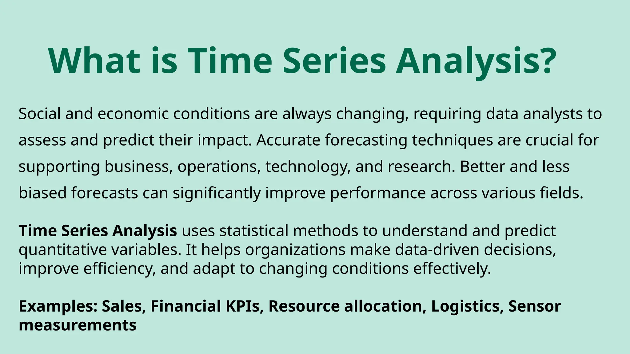
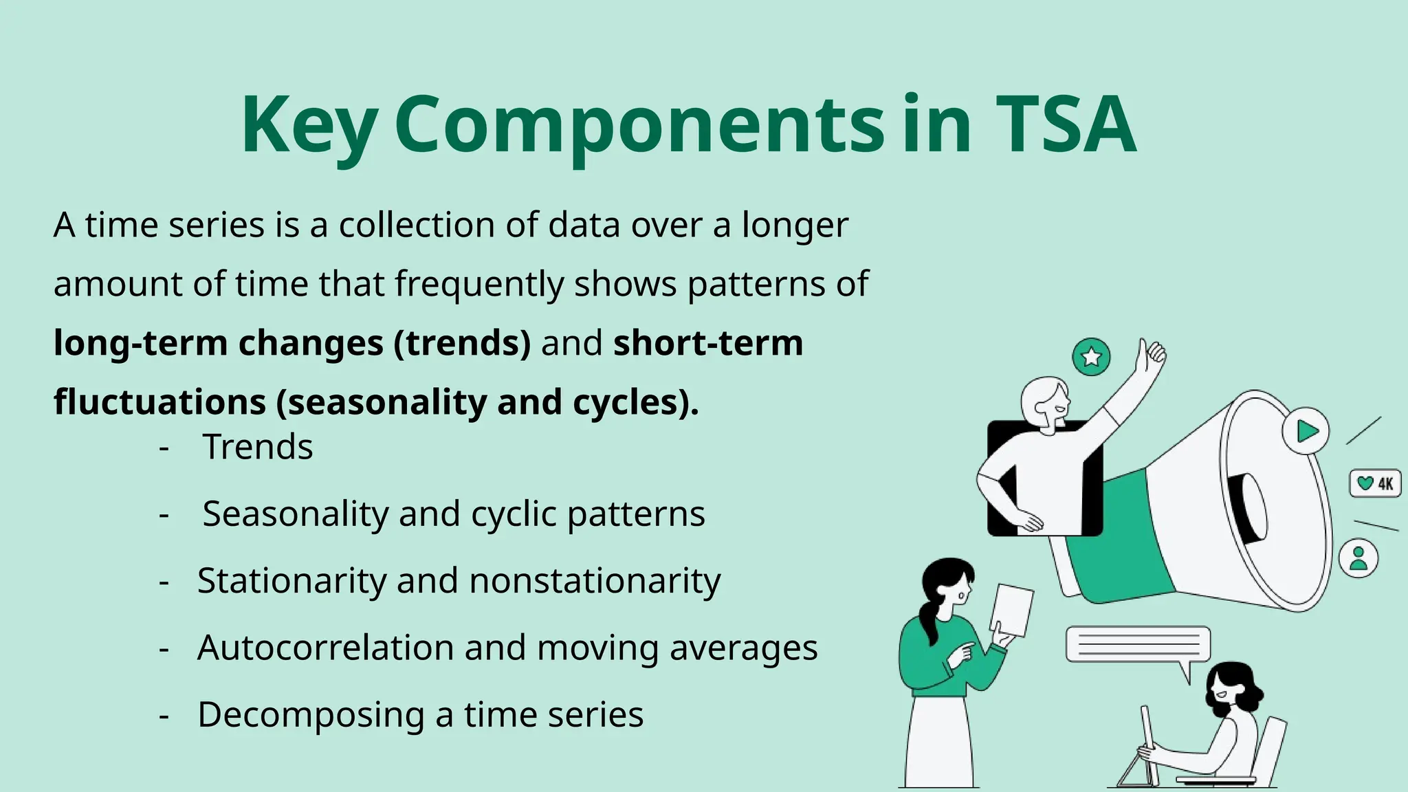
Presentation On Time Series Analysis in Mechine Learning

Course: Big Data Analytics
Course Code: CSE-5110
Jagannath University (15th Batch)
ID: M240105050
Course: Big Data Analytics
Time Series Analysis

Presented To:
Dr. Md. Monwarul Islam (MMI)
Associate Professor
Department of Computer Science and Engineering
Jagannath University
Presented By:
Adri Saha
ID: M240105050
Department of Computer Science and Engineering
Jagannath University

What is Time Series Analysis?
Social and economic conditions are always changing, requiring data analysts to
assess and predict their impact. Accurate forecasting techniques are crucial for
supporting business, operations, technology, and research. Better and less
biased forecasts can significantly improve performance across various fields.
Time Series Analysis uses statistical methods to understand and predict
quantitative variables. It helps organizations make data-driven decisions,
improve efficiency, and adapt to changing conditions effectively.
Examples: Sales, Financial KPIs, Resource allocation, Logistics, Sensor
measurements

1. Graphical and numerical summary: Displays data
points over time.
2. Interpretation of series features: Analyzes patterns
like seasonality, trends and relationships with other
data series.
3. Forecasting: Predicts future values of the series like at
t+1,t+2,…,t+n).
4. Hypothesis testing and simulation: Compares
different scenarios to evaluate outcomes.
Why analyze Time series
data?

Applications of TSA
Manufacturing
Logistics &
Transportation
Retailgrocery
Insurance
Energy &
Utilities
Predictive maintenance: Enhances operational efficiency.
Shipped packages forecasting: Supports workforce planning.
Sales forecasting during promotions: Optimizes warehouse
management.
Claims prediction: Helps determine suitable insurance
policies.
Energy load forecasting: Improves planning and trading
strategies.

Key Components in TSA
- Trends
- Seasonality and cyclic patterns
- Stationarity and nonstationarity
- Autocorrelation and moving averages
- Decomposing a time series
A time series is a collection of data over a longer
amount of time that frequently shows patterns of
long-term changes (trends) and short-term
fluctuations (seasonality and cycles).

Trends
1. The trend in a time series represents the overall
direction of the data over a long period. It
indicates whether there is a sustained long-term
increase or decrease in the values.
2. The trend does not have to be linear. It can also be
exponential or follow other functional forms.
Cycle
1. Long-term, regular fluctuations by repeated upward
or downward swings.
2. Duration: Vary, usually from 2 to 20 or even thirty
years.
3. Detection can be challenging to identify as it is often
confused with the trend component.

Seasonality
Predictable: Occurs due to factors like weather, holidays or
economic cycles.
Example: Weekly seasonality (Newspaper daily sales)
01 Patterns: Repeating patterns at fixed intervals (E.g. daily,
monthly, yearly).
02
.

(i)Mean: E(Yt) = μ
(ii)Variance: var(Yt) = E( Yt – μ)2
= σ2
(iii)Covariance: γk = E[(Yt – μ)(Yt-k –
μ)2
Forms of Stationarity: weak, strong (strict), super
(Engle, Hendry, & Richard 1983)
Testing for
Stationarity

Types of Stationary
• If the mean and variance of a time series remain constant throughout
time and the covariance between two time points varies only on their
distance from one another, then the time series is considered to be
weakly stationary.
• A time series is strongly stationary if the joint distribution of any set of
points in the series depends only on the gaps between them and not on
the specific time at which they occur.
• If a weakly stationary series follows a normal (Gaussian) distribution, it
is also considered strongly stationary. This is why we often check
whether a time series follows a normal distribution.

Stationary Vs Non-
Stationary
• Similarly to significant occurrences like 9/11 and Watergate, shocks only
have short-term effects on a stationary series until it eventually recovers
to its long-term average. However, for a non-stationary series, shocks
cause permanent shifts away from the long-term average.
• A stationary series has a variance or data spread which does not
change over time. However, over time, the variance of a non-stationary
series grows and becomes infinite.

Correlation of a signal with a
delayed copy of itself
Helps identify repeating patterns or
seasonality
Tools: Autocorrelation Function
(ACF), Partial Autocorrelation
Function (PACF)
Autocorrelatio
n

Auto Correlated Function (ACF)
Example (Presidential Approval)

Autocorrelated Functions (ACF)
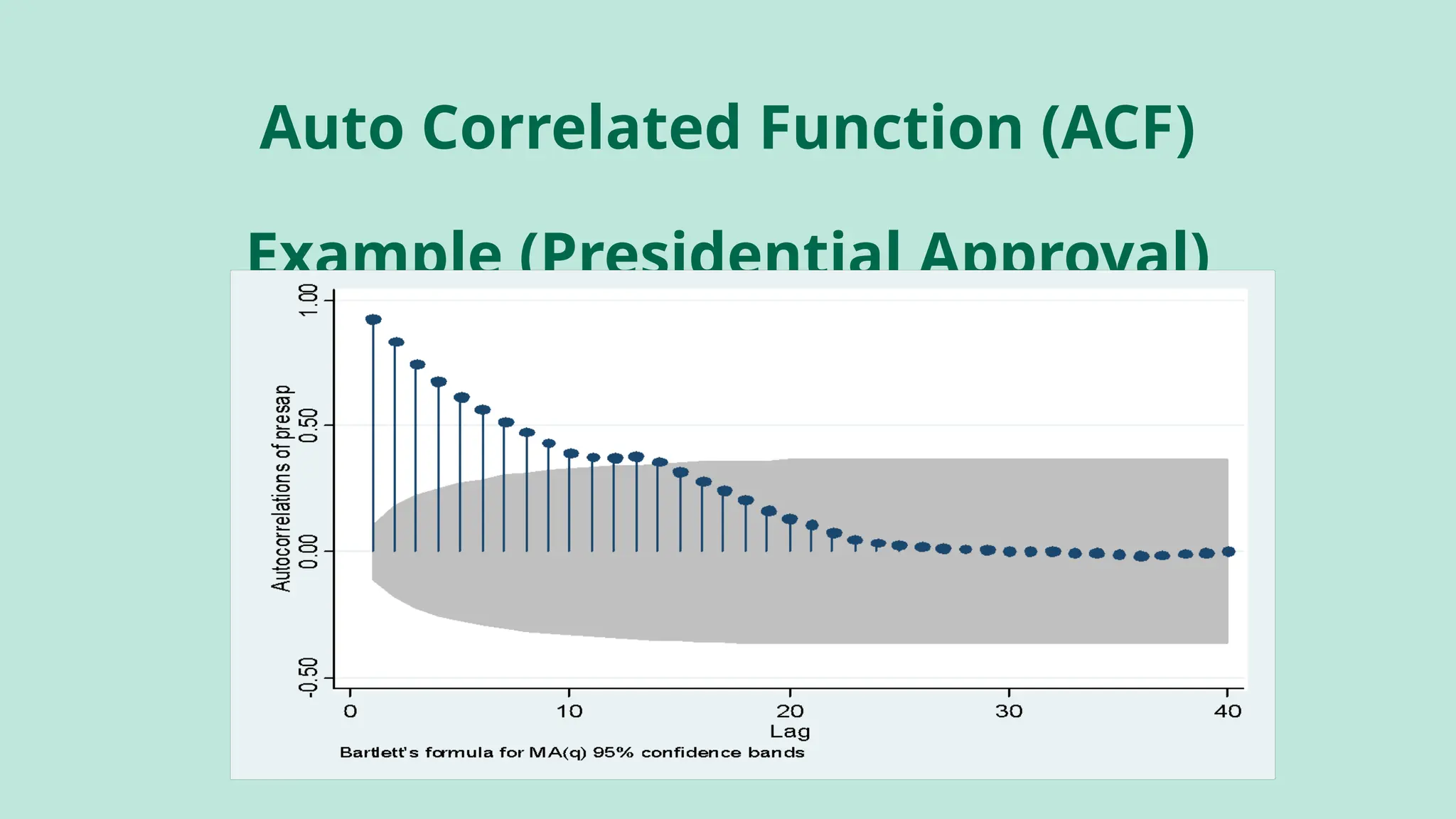
The ACF shows how persistent a variable is over its relative delays.
ρk = γk / γ0 = covariance at lag k
variance
ρk = E[(yt – μ)(yt-k – μ)]2
E[(yt – μ)2
]
ACF (0) = 1, ACF (k) = ACF (-k)
Explanation
The approval series shows a long-lasting effect. Even though it doesn't
have a unit root, it has long memory, meaning that shocks to the series
last for at least 12 months.
If the ACF (Autocorrelation Function) shows a hyperbolic pattern, it
might mean the series is fractionally integrated.

Breaking Down a Time Series:
Time series can be decomposed into:
1. Trend component
2. Seasonal component
3. Remainder (residual)
4. This helps in understanding underlying patterns
and making forecasts.
Time Series
Decomposition

Used for smoothing time series and identifying
trends.
Moving Averages
01.
Simple
Moving
Average
(SMA)
02. 03.
Weighted
Moving
Average
(WMA)
Exponential
Moving
Average
(EMA)

Working Flow
Data Collection: Gather time-based data.
Data Preprocessing: Clean and prepare the data
(handling missing values, normalization).
Exploratory Analysis: Visualize data to identify trends,
seasonality, and patterns.
Modeling: Choose and apply suitable algorithms.
Validation: Test the model's accuracy.
Prediction: Use the model to forecast future data points.
Evaluation: Assess model performance and refine it as
needed.

Traditional
- Exponential smoothing (ETS)
- ARIMA models
- SARIMA (Seasonal ARIMA)
Advanced
- Prophet Model
- Spectral analysis
Machine/deep learning models
- Random Forest, SVM
- LSTM (Long Short-Term Memory Networks)
Some TSA models
01.
02.
03.

Methods
✔ Simple Exponential Smoothing
✔ Double Exponential Smoothing (Holt's
method)
✔ Triple Exponential Smoothing (Holt-
Winters' method)
Exponential Smoothing

Exponential Smoothing Vs ARIMA
Exponential smoothing methods are concerned with describing the level
of data, trend, and seasonality, whereas ARIMA models try to identify and
explain the autocorrelations in the data.
ARIMA Model describes how past observations of a target variable are
statistically correlated with its future values.
Flexible forecasting model that can be applied to time series data by making
it stationary through methods like differencing and lagging. An ARIMA
model includes:
Autoregressive (AR): Captures relationships with past values.
Moving Average (MA): Accounts for past forecast errors.
Integration (I): Handles the differencing needed to make the series
stationary.
So that the model is called ARIMA (Auto Regressive Integrated Moving

How ARIMA Works
Step 1: Identification: Find out if there is a stationary
series. Use differencing if not.
Step 2: Model Selection: Choose AR, I, and MA terms
(parameters p, d, q) using techniques like ACF and PACF
plots.
Step 3: Estimation: Fit the ARIMA model to the data.
Step 4: Forecasting: Use the fitted model to predict future
values
Eg: ARIMA(1,1,1): Uses 1 lag for autoregression, 1
differencing to make the series stationary and 1 lag for the
moving average.

Handling Seasonality with SARIMA:
•Extension of ARIMA for seasonal time series
•Incorporates seasonal differencing
•Useful for data with clear seasonal patterns.
Seasonal
ARIMA
(SARIMA)

LSTM Networks for Time Series:
•Type of Recurrent Neural Network (RNN)
•Capable of learning long-term dependencies
•Useful for complex time series with multiple
input variables.
Long Short-Term
Memory (LSTM)

ARIMA (Autoregressive
Integrated Moving
Average):
oFocused on single
series estimation
oWidely used for
forecasting.
oCombines
autoregression,
differencing and
moving average.
SARIMA (Seasonal
ARIMA):
oExtension of
ARIMA.
oAccounts for
seasonality in data.
LSTM (Long Short-
Term Memory
Networks):
oA type of recurrent
neural network.
oEffective for
handling long-term
dependencies in
time series data.

Facebook's Prophet Model:
•Designed for business forecasting
•Handles daily observations with strong
seasonal effects
•Robust to missing data and shifts in trend
Prophet Model

Time Series Cross-
Validation
Traditional cross-validation doesn't work for time
series
Use techniques like rolling forecast origin
Metrics: Mean Absolute Error (MAE), Root Mean
Squared Error (RMSE)

Dealing with Missing Values:
• Linear interpolation
• Last observation carried forward (LOCF)
• Mean/median imputation
• More advanced methods: multiple
imputation, KNN imputation
Handling Missing Data

Feature Engineering
for Time Series
Creating Relevant Features:
•Lag features
•Rolling window statistics
•Date-based features (day of week,
month, etc.)
•Domain-specific indicators

Analyzing Multiple Time Series:
Multivariate Time
Series
•Vector Autoregression (VAR)
•Dynamic Factor Models
•Multivariate LSTM networks

Advanced Topic : VAR
•VAR (Vector Autoregression) is a helpful model in which all
variables are viewed as endogenous (they influence one
another).
•If there are 3 variables, the model creates 3 equations, each
including lags of all the variables.
•Once the system is estimated, you can analyze how one
variable reacts when another variable experiences a shock (a
sudden change from its average).

Grouping Similar Time Series:
✔ Dynamic Time Warping (DTW) for similarity
measurement
✔ K-means clustering with DTW
✔ Hierarchical clustering of time series
Time Series Clustering

Future Trends in TSA
Emerging Directions:
•Deep learning approaches for complex time series
•Integration with big data technologies.
•Real-time analysis and forecasting.
•Explainable AI in time series forecasting

Thank
you very
much!
Presented by Adri Saha

REFERENCES
1.M. de Gooijer, G. Ray, and M. Schmidt, "A Comprehensive Review on Time Series
Forecasting Using Deep Learning," ScienceDirect, 2021. Available at:
https://www.sciencedirect.com/science/article/pii/S0169207021001758.
2.Penn State Eberly College of Science, "Lesson 1: Introduction to Time Series
Analysis," STAT 510, Available at:
https://online.stat.psu.edu/stat510/lesson/1/1.2.
3.Stack Exchange, "Weakly Stationary Gaussian AR(1) Process is Strict
Stationary?" Available at: https://stats.stackexchange.com/questions/483463/.
4.Hyndman, R. J. and Athanasopoulos, G., "Stationarity," Forecasting: Principles
and Practice, 2nd ed., Available at: https://otexts.com/fpp2/stationarity.html.

Presentation On Time Series Analysis in Mechine Learning

More Related Content

What's hot

Similar to Presentation On Time Series Analysis in Mechine Learning

Recently uploaded

Presentation On Time Series Analysis in Mechine Learning

Editor's Notes