Time Series Analysis and Forecasting.ppt

Time Series Analysis and
Forecasting

Introduction to Time Series Analysis
• A time-series is a set of observations on a quantitative variable
collected over time.
• Examples
– Dow Jones Industrial Averages
– Historical data on sales, inventory, customer counts, interest
rates, costs, etc
• Businesses are often very interested in forecasting time series
variables.
• Often, independent variables are not available to build a
regression model of a time series variable.
• In time series analysis, we analyze the past behavior of a
variable in order to predict its future behavior.

Methods used in Forecasting
• Regression Analysis
• Time Series Analysis (TSA)
– A statistical technique that uses time-
series data for explaining the past or
forecasting future events.
– The prediction is a function of time
(days, months, years, etc.)
– No causal variable; examine past behavior
of a variable and and attempt to predict
future behavior

Components of TSA
• Time Frame (How far can we predict?)
– short-term (1 - 2 periods)
– medium-term (5 - 10 periods)
– long-term (12+ periods)
– No line of demarcation
• Trend
– Gradual, long-term movement (up or down) of
demand.
– Easiest to detect

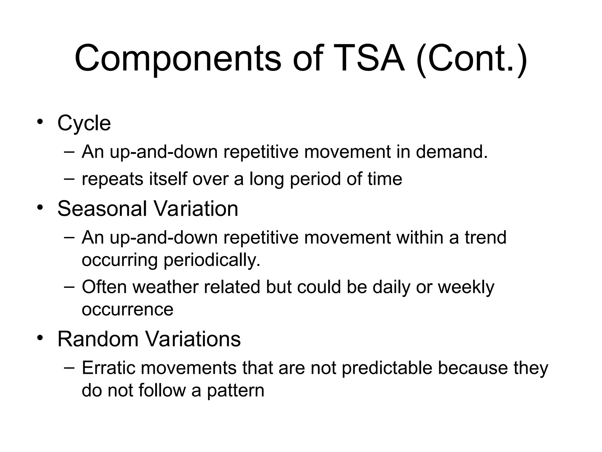
Components of TSA (Cont.)
• Cycle
– An up-and-down repetitive movement in demand.
– repeats itself over a long period of time
• Seasonal Variation
– An up-and-down repetitive movement within a trend
occurring periodically.
– Often weather related but could be daily or weekly
occurrence
• Random Variations
– Erratic movements that are not predictable because they
do not follow a pattern

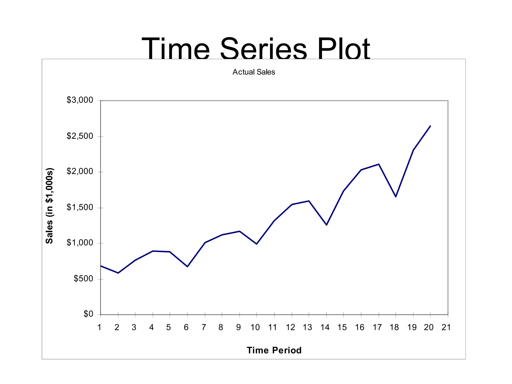
Time Series Plot
Actual Sales
$0
$500
$1,000
$1,500
$2,000
$2,500
$3,000
1 2 3 4 5 6 7 8 9 10 11 12 13 14 15 16 17 18 19 20 21
Time Period
Sales
(in
$1,000s)

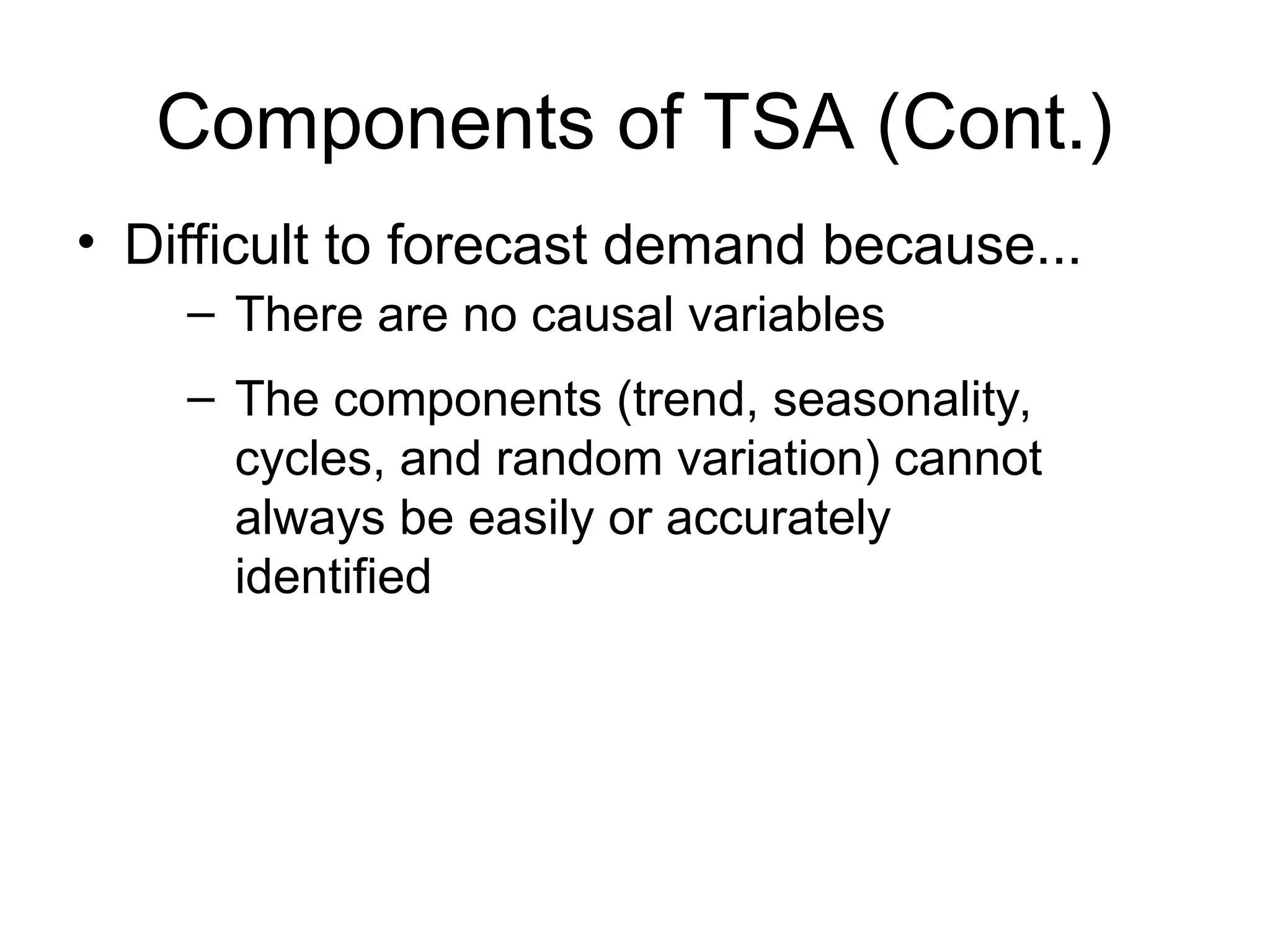
Components of TSA (Cont.)
• Difficult to forecast demand because...
– There are no causal variables
– The components (trend, seasonality,
cycles, and random variation) cannot
always be easily or accurately
identified

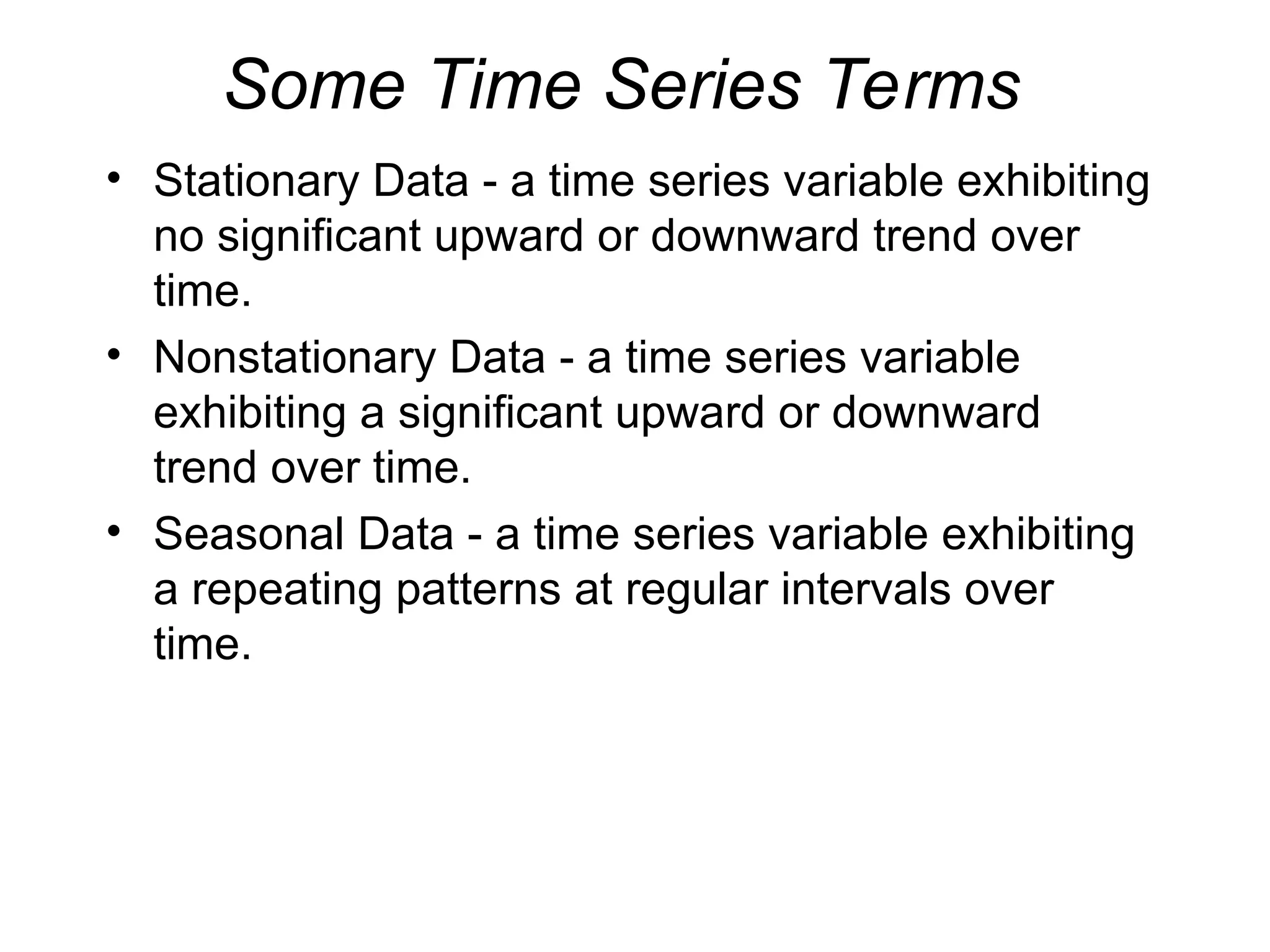
Some Time Series Terms
• Stationary Data - a time series variable exhibiting
no significant upward or downward trend over
time.
• Nonstationary Data - a time series variable
exhibiting a significant upward or downward
trend over time.
• Seasonal Data - a time series variable exhibiting
a repeating patterns at regular intervals over
time.

Approaching Time Series Analysis
• There are many, many different time series
techniques.
• It is usually impossible to know which technique
will be best for a particular data set.
• It is customary to try out several different
techniques and select the one that seems to
work best.
• To be an effective time series modeler, you need
to keep several time series techniques in your
“tool box.”

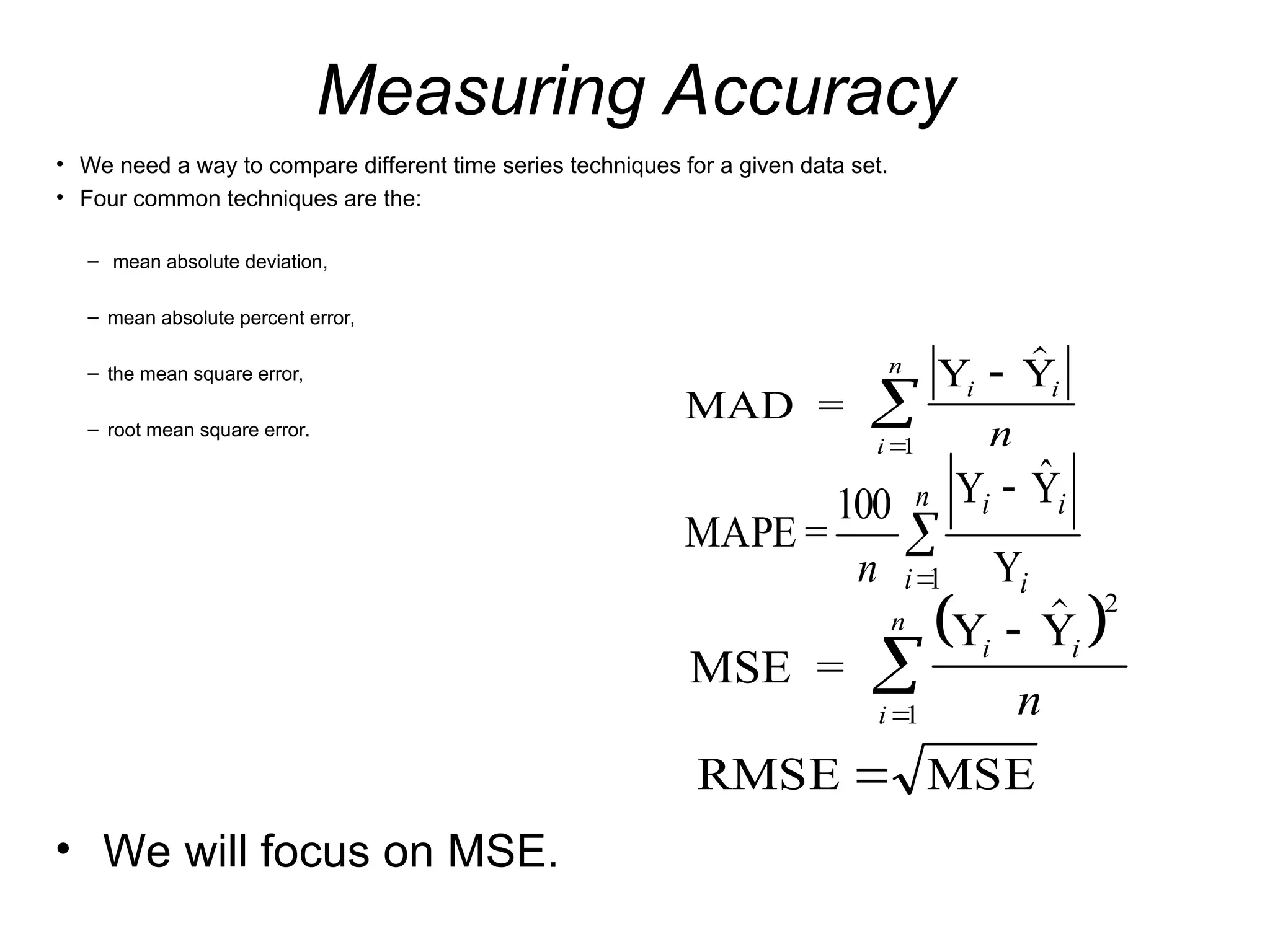
Measuring Accuracy
• We need a way to compare different time series techniques for a given data set.
• Four common techniques are the:
– mean absolute deviation,
– mean absolute percent error,
– the mean square error,
– root mean square error.
MAD =
Y Y
i i
i
n
n




1
 
MSE =
Y Y
i i
i
n
n



 2
1
MSE
RMSE 



n
i i
i
i
n 1 Y
Ŷ
Y
100
=
MAPE
• We will focus on MSE.

Extrapolation Models
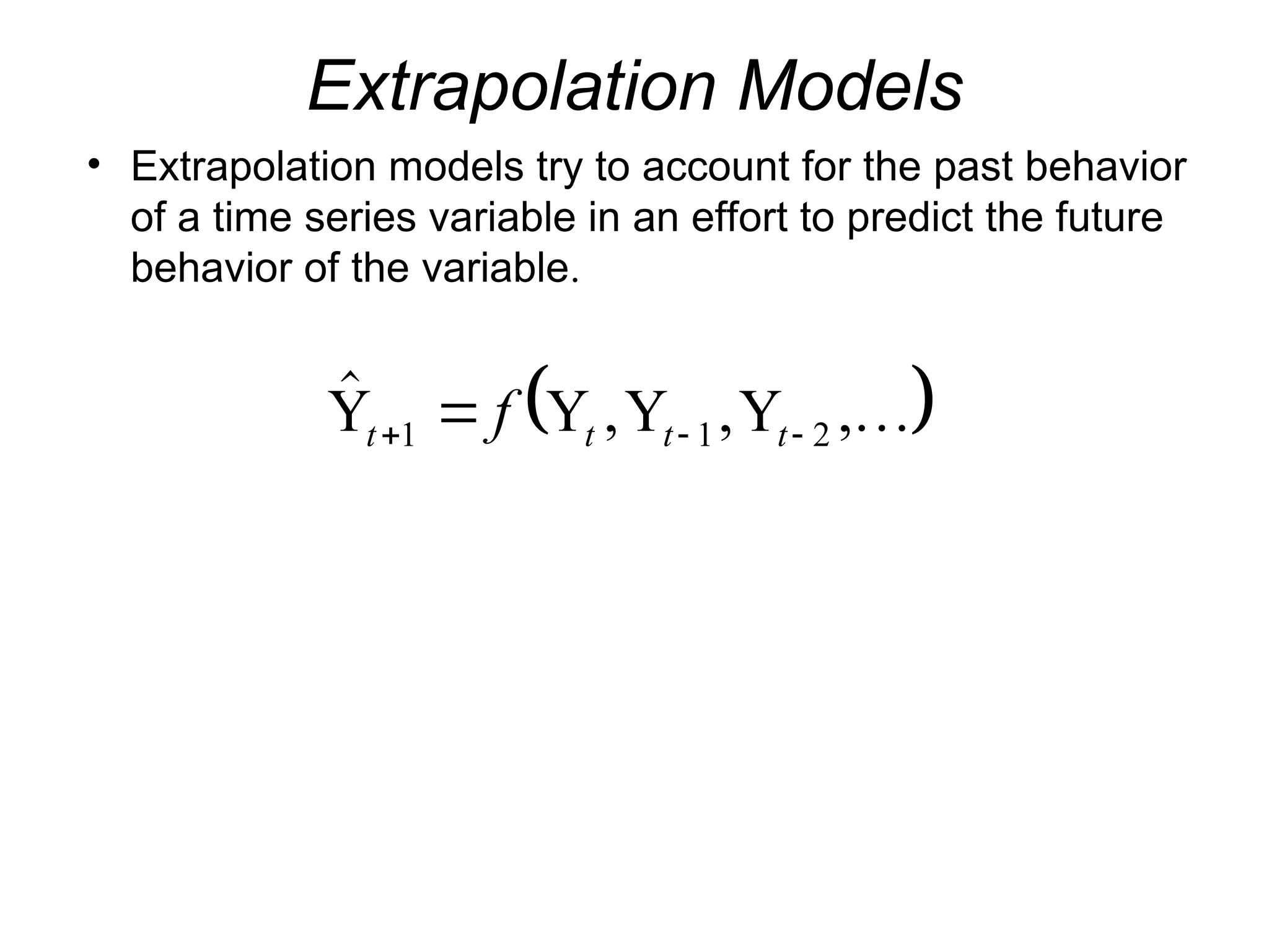
• Extrapolation models try to account for the past behavior
of a time series variable in an effort to predict the future
behavior of the variable.
 
 , , ,
Y Y Y Y
t t t t
f
  

1 1 2 

Moving Averages

Y
Y Y Y
t t-1 t- +1
t
k
k
 
 
1
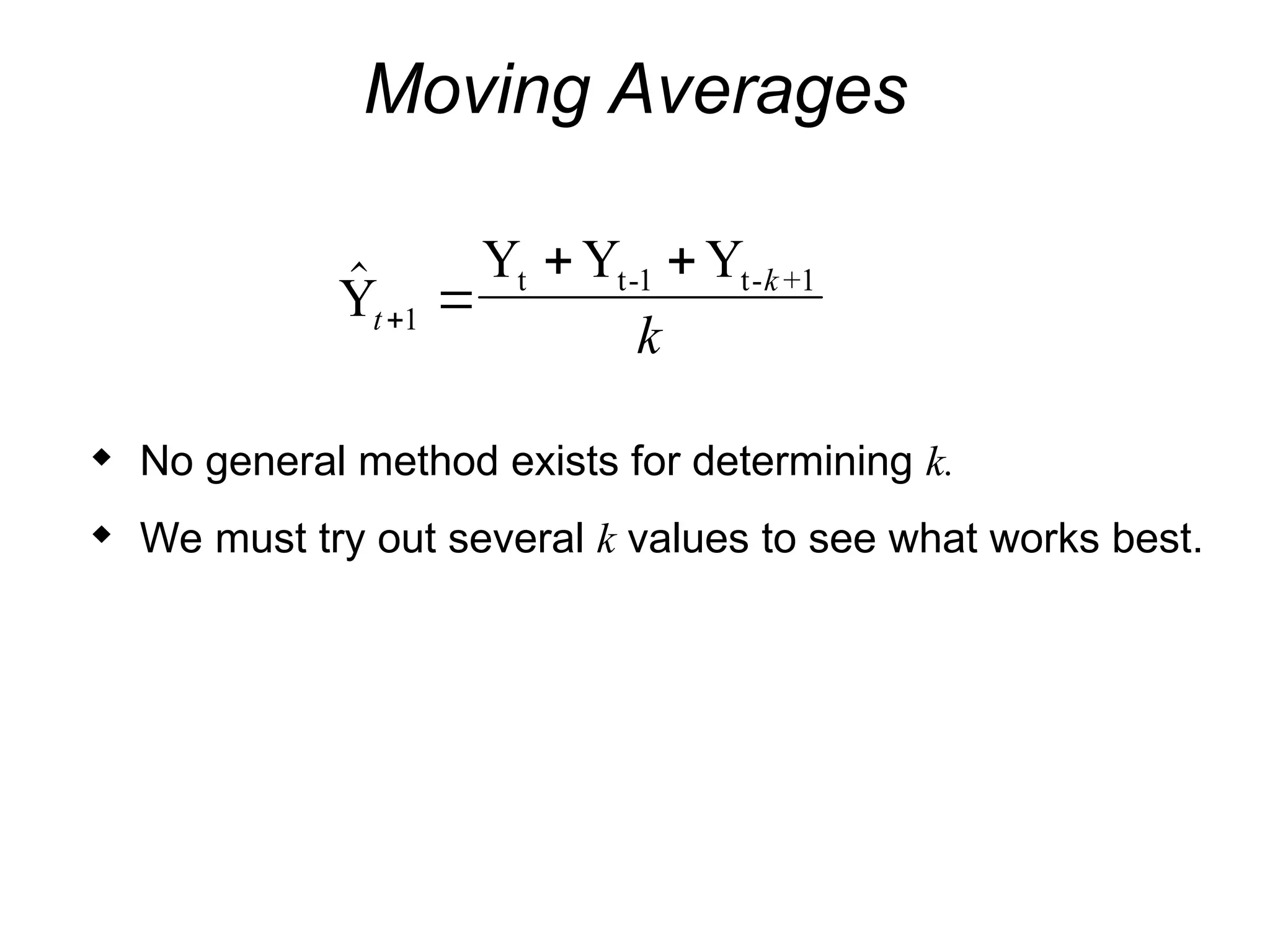
 No general method exists for determining k.
 We must try out several k values to see what works best.

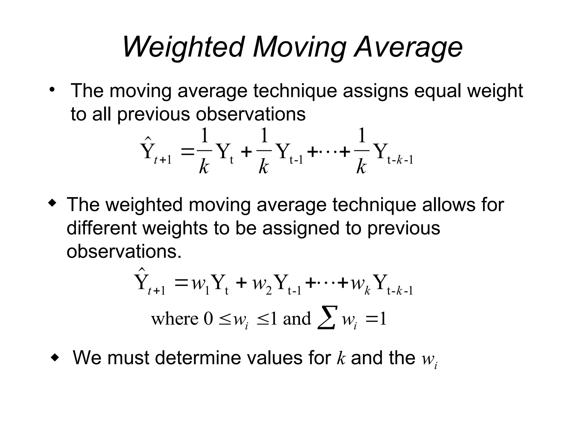
Weighted Moving Average
• The moving average technique assigns equal weight
to all previous observations

Y
1
Y
1
Y
1
Y
t t-1 t- -1
t k
k k k
    
1 
 The weighted moving average technique allows for
different weights to be assigned to previous
observations.

Y Y Y Y
t t-1 t- -1
t k k
w w w
    
1 1 2 
where 0 and
  

w w
i i
1 1
 We must determine values for k and the wi

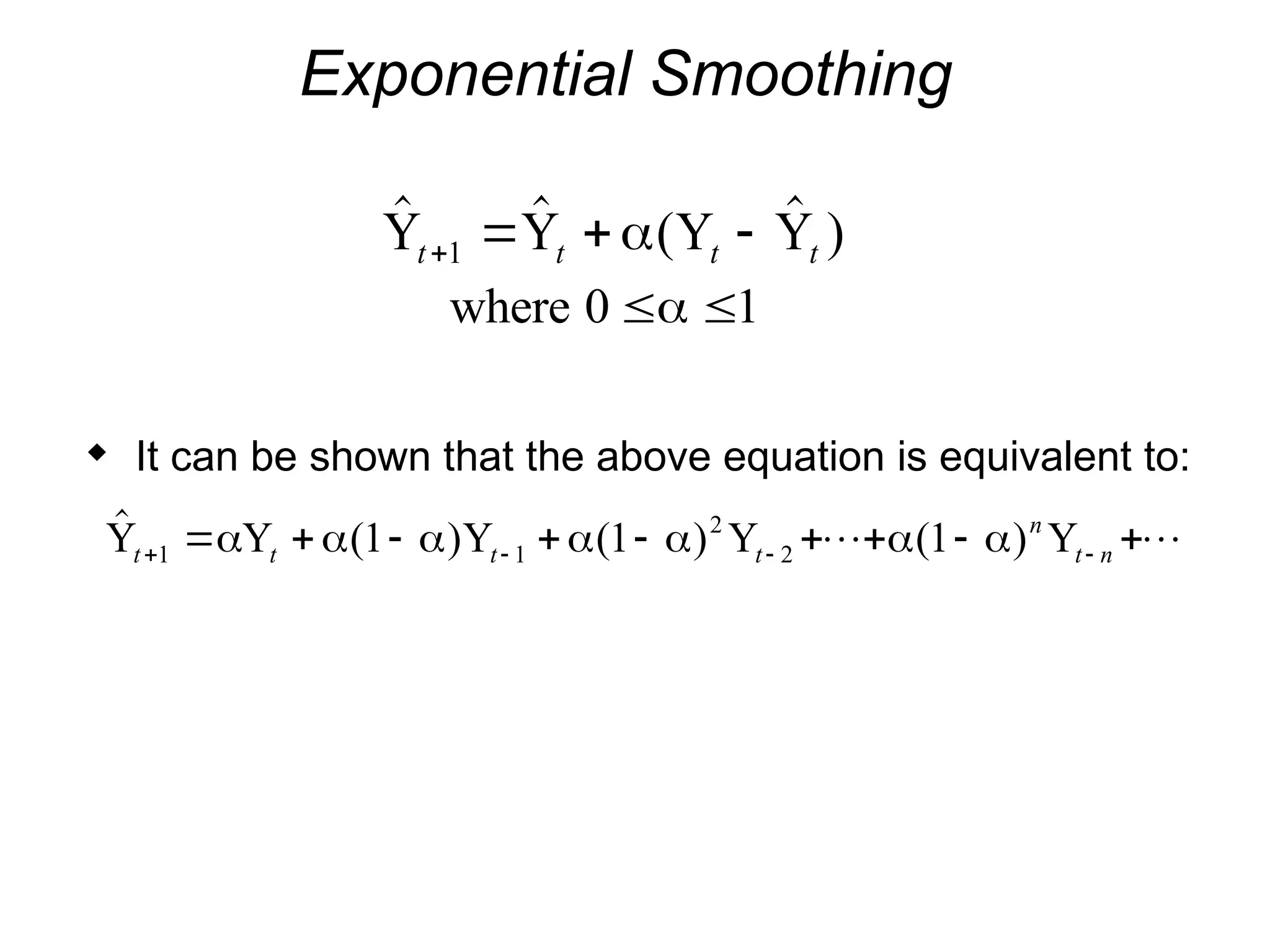
Exponential Smoothing
  (  )
Y Y Y Y
t t t t
   
1 
where 0 1
 

 It can be shown that the above equation is equivalent to:
 ( ) ( ) ( )
Y Y Y Y Y
t t t t
n
t n
   
        
1 1
2
2
1 1 1
      
 

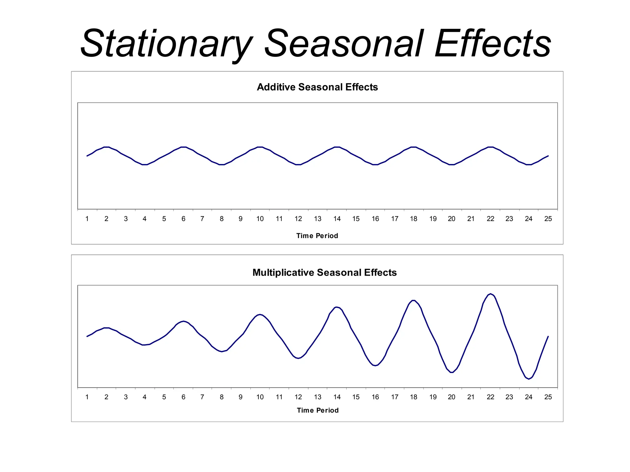
Seasonality
• Seasonality is a regular, repeating
pattern in time series data.
• May be additive or multiplicative in
nature...

Multiplicative Seasonal Effects
1 2 3 4 5 6 7 8 9 10 11 12 13 14 15 16 17 18 19 20 21 22 23 24 25
Time Period
Additive Seasonal Effects
1 2 3 4 5 6 7 8 9 10 11 12 13 14 15 16 17 18 19 20 21 22 23 24 25
Time Period
Stationary Seasonal Effects

Trend Models
• Trend is the long-term sweep or general
direction of movement in a time series.
• We’ll now consider some nonstationary time
series techniques that are appropriate for
data exhibiting upward or downward trends.

The Linear Trend Model

Y X
t b b t
 
0 1 1
where X1t
t

For example:
X X X
1 1 1
1 2 3
1 2 3
  
, , , 

The TREND() Function
TREND(Y-range, X-range, X-value for prediction)
where:
Y-range is the spreadsheet range containing the dependent Y
variable,
X-range is the spreadsheet range containing the independent X
variable(s),
X-value for prediction is a cell (or cells) containing the values for
the independent X variable(s) for which we want an estimated value
of Y.
Note: The TREND( ) function is dynamically updated whenever any inputs to
the function change. However, it does not provide the statistical information
provided by the regression tool. It is best two use these two different
approaches to doing regression in conjunction with one another.

The Quadratic Trend Model

Y X X
t b b b
t t
  
0 1 1 2 2
where X and X
1 2
2
t t
t t
 

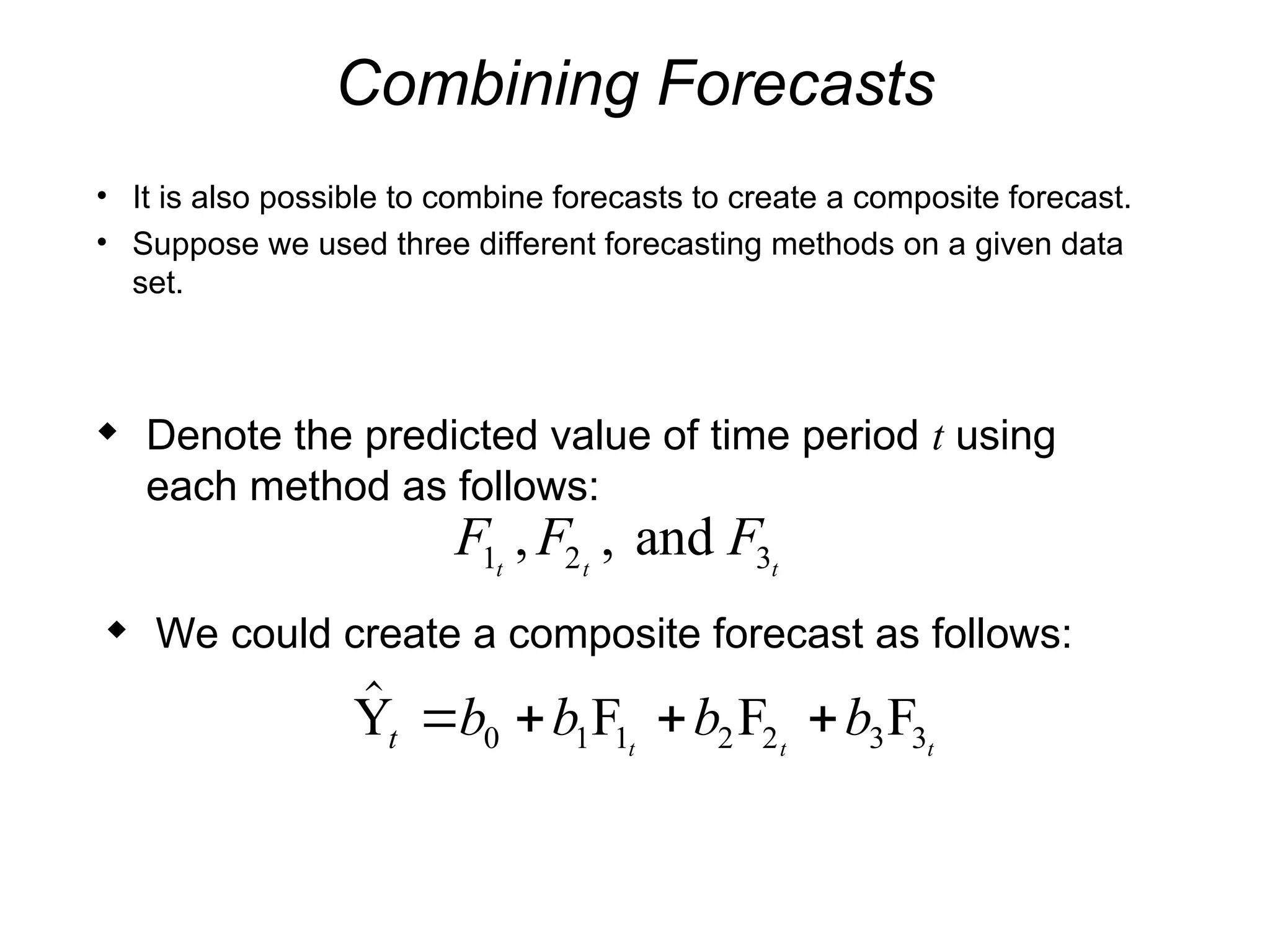
Combining Forecasts
• It is also possible to combine forecasts to create a composite forecast.
• Suppose we used three different forecasting methods on a given data
set.
 Denote the predicted value of time period t using
each method as follows:
F F F
t t t
1 2 3
, , and
 We could create a composite forecast as follows:

Y F F F
t b b b b
t t t
   
0 1 1 2 2 3 3

Time Series Analysis and Forecasting.ppt

More Related Content

Similar to Time Series Analysis and Forecasting.ppt

Recently uploaded

Time Series Analysis and Forecasting.ppt