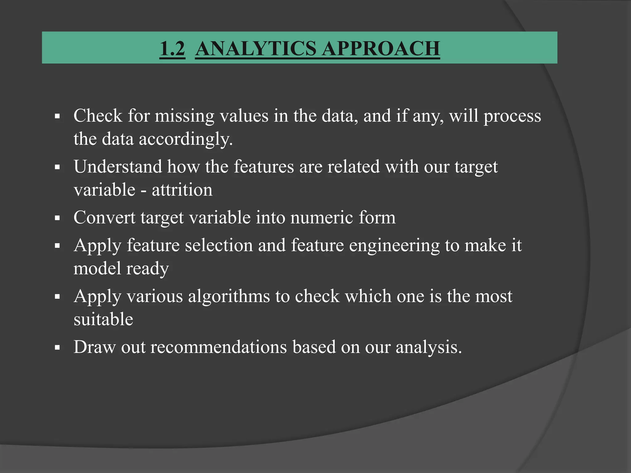
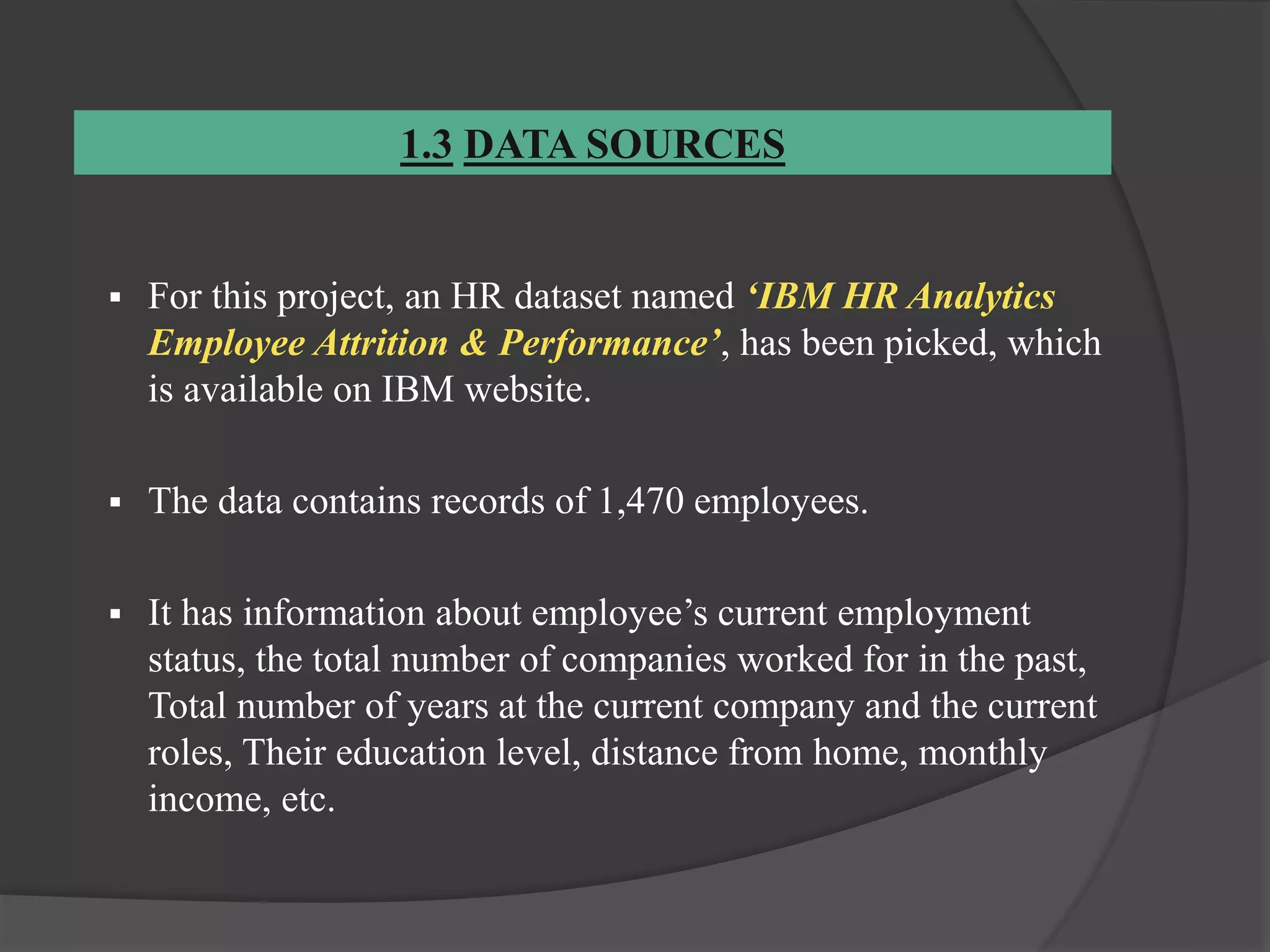
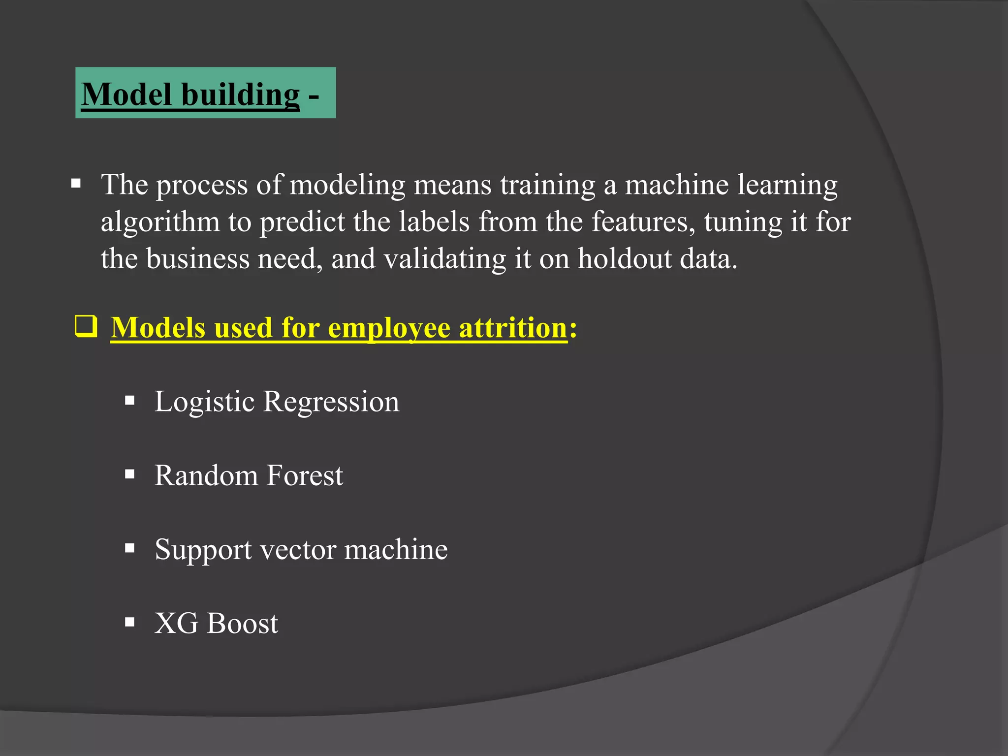
Predicting Employee Attrition

1.1 OBJECTIVE AND SCOPE OF THE STUDY
 The objective of this project is to predict the attrition rate for
each employee, to find out who’s more likely to leave the
organization.
 It will help organizations to find ways to prevent attrition or
to plan in advance the hiring of new candidate.
 Attrition proves to be a costly and time consuming problem
for the organization and it also leads to loss of productivity.
 The scope of the project extends to companies in all
industries.

1.2 ANALYTICS APPROACH
 Check for missing values in the data, and if any, will process
the data accordingly.
 Understand how the features are related with our target
variable - attrition
 Convert target variable into numeric form
 Apply feature selection and feature engineering to make it
model ready
 Apply various algorithms to check which one is the most
suitable
 Draw out recommendations based on our analysis.

1.3 DATA SOURCES
 For this project, an HR dataset named ‘IBM HR Analytics
Employee Attrition & Performance’, has been picked, which
is available on IBM website.
 The data contains records of 1,470 employees.
 It has information about employee’s current employment
status, the total number of companies worked for in the past,
Total number of years at the current company and the current
roles, Their education level, distance from home, monthly
income, etc.

1.4 TOOLS AND TECHNIQUES
 We have selected Python as our analytics tool.
 Python includes many packages such as Pandas, NumPy,
Matplotlib, Seaborn etc.
 Algorithms such as Logistic Regression, Random Forest,
Support Vector Machine and XGBoost have been used for
prediction.

 Importing Libraries
2.1 IMPORTING LIBRARY AND DATA EXTRACTION

 Importing Packages
 Data Extraction

2.2 EXPLORATORY DATA ANALYSIS
 Refers to the process of performing initial investigations on the
data so as to discover patterns, to spot inconsistencies, to test
hypothesis and to check assumptions with the help of graphical
representations
 Displaying First 5 Rows

 Displaying rows and columns

 Identifying Missing Values

 Count of “Yes” and “No” values of Attrition

2.3 VISUALIZATION(EDA) -
 Attrition V/s “Age”

 Attrition V/s “Distance from Home”

 Attrition V/s “Job Satisfaction”

 Attrition V/s “Performance Rating”

 Attrition V/s “Training Times Last Year”

 Attrition V/s “Work Life Balance”

 Attrition V/s “Years At Company”

 Attrition V/s “Years in Current Role”

 Attrition V/s “Years Since Last Promotion”

 Attrition V/s Categorical Variables

Attrition V/s “Gender, Marital status and Overtime”

Attrition V/s “Department, Job Role, and Business Travel”

Data Pre-Processing-
Steps Involved –
 Taking care of missing data and dropping non-relevant
features
 Feature extraction
 Converting categorical features into numeric form
Binarization of the converted categorical features
 Feature scaling
 Understanding correlation of features with each other
 Splitting data into training and test data sets
 Refers to data mining technique that transforms raw data into
an understandable format
 Useful in making the data ready for analysis

3.1 FEATURE SELECTION
 Process wherein those features are selected, which contribute
most to the prediction variable or output.
Benefits of feature selection :
 Improve the performance
 Improves Accuracy
 Providing the better understanding of Data

Dropping non-relevant variables
#dropping all fixed and non-relevant variables
attrition_df.drop(['DailyRate','EmployeeCount','EmployeeNumber','HourlyRate','Month
lyRate','Over18','PerformanceRating','StandardHours','StockOptionLevel','TrainingTi
mesLastYear'], axis=1,inplace=True)
Check number of rows and columns

Features Extraction
3.2 FEATURE ENGINEERING

Label Encoding
 Label Encoding refers to converting the categorical variables into numeric
form, so as to convert it into the machine-readable form.
 It is an important pre-processing step for the structured dataset in supervised
learning.
 Fit and transform the required columns of the data, and then replace the
existing text data with the new encoded data.

Convert categorical variables into numeric variables

 One Hot Encoder
 It is used to perform “binarization” of the categorical features and
include it as a feature to train the model.
 It takes a column which has categorical data that has been label
encoded, and then splits the column into multiple columns.
 The numbers are replaced by 1s and 0s, depending on which
column has what value.

Applying “One Hot Encoder” on Label Encoded features

Feature Scaling
 Feature scaling is a method used to standardize the range of
independent variables or features of data
 It is also known as Data Normalization
 It is used to scale the features to a range which is centred around
zero so that the variance of the features are in the same range
 Two most popular methods of feature scaling are standardization
and normalization

Correlation Matrix
• Correlation is a statistical technique which determines how one
variables moves/changes in relation with the other variable.
• It’s a bi-variant analysis measure which describes the association
between different variables.
Usefulness of Correlation matrix –
 If two variables are closely correlated, then we can predict one
variable from the other.
 Correlation plays a vital role in locating the important variables
on which other variables depend.
 It is used as the foundation for various modeling techniques.
 Proper correlation analysis leads to better understanding of data.

Plotting correlation matrix

Splitting data into train and test

 The process of modeling means training a machine learning
algorithm to predict the labels from the features, tuning it for
the business need, and validating it on holdout data.
 Models used for employee attrition:
 Logistic Regression
 Random Forest
 Support vector machine
 XG Boost
Model building -

4.1 LOGISTIC REGRESSION
 Logistic Regression is one of the most basic and widely used
machine learning algorithms for solving a classification problem.
 It is a method used to predict a dependent variable (Y), given an
independent variable (X), given that the dependent variable
is categorical.

 Linear Regression equation
 Y stands for the dependent variable that needs to be predicted.
 β0 is the Y-intercept, which is basically the point on the line which
touches the y-axis.
 β1 is the slope of the line (the slope can be negative or positive
depending on the relationship between the dependent variable and
the independent variable.)
 X here represents the independent variable that is used to predict
our resultant dependent value.
 ∈ denotes the error in the computation

 Sigmoid Function
p(x)= β0+ β1x

 Building Logistic Regression Model

 Confusion Matrix
 Confusion matrix is the most crucial metric commonly used to
evaluate classification models.
 The confusion matrix avoids "confusion" by measuring the
actual and predicted values in a tabular format.
In table above, Positive class = 1 and Negative class = 0.
Standard table of confusion matrix -

 Creating confusion matrix
 AUC score

 Receiver Operator Characteristic (ROC)
 ROC determines the accuracy of a classification model at a user
defined threshold value.
 It determines the model's accuracy using Area Under Curve
(AUC).
 The area under the curve (AUC), also referred to as index of
accuracy (A) or concordant index, represents the performance of
the ROC curve. Higher the area, better the model.

 ROC Curve For Logistic Regression
Using Logistic Regression algorithm, we got the accuracy score of
79% and roc_auc score of 0.77

4.2 RANDOM FOREST
• Random Forest is a supervised learning algorithm.
• It creates a forest and makes it random based on bagging
technique. It aggregates Classification Trees.
• In Random Forest, only a random subset of the features is taken
into consideration by the algorithm for splitting a node.

 Building Random Forest Model

 Testing the Model

 AUC score
 Plotting ROC curve

Using Random Forest algorithm, we got the accuracy score of 79%
and roc_auc score of 0.76.
 ROC Curve For Random Forest

4.3 SUPPORT VECTOR MACHINE
 SVM is a supervised machine learning algorithm used for both
regression and classification problems.
 Objective is to find a hyperplane in an N -dimensional space.
 Hyperplanes
 Hyperplanes are decision boundaries
that help segregate the data points.
 The dimension of the hyperplane
depends upon the number of features.

 Support Vectors
 These are data points that are closest to the hyperplane and
influence the position and orientation of the hyperplane.
 Used to maximize the margin of the classifier.
 Considered as critical elements of a dataset

 Kernel Technique
 Used when non-linear hyperplanes are needed
 The hyperplane is no longer a line, it must now be a plane
 Since we have a non-linear
classification problem, kernel
technique used here is Radial Basis
Function (rbf)
 Helps in segregating data that are
linearly non-separable.

 Testing SVM Model

 AUC Score
 Plotting ROC Curve

Using SVM algorithm, we got the accuracy score of 79% and
roc_auc score of 0.77
 ROC Curve For SVM

4.4 XG BOOST
 XGBoost is a decision-tree-based ensemble Machine Learning algorithm
that uses a gradient boosting framework.
 XGBoost belongs to a family of boosting algorithms that convert weak
learners into strong learners.
 It is a sequential process, i.e., trees are grown using the information from
a previously grown tree one after the other, iteratively, the errors of the
previous model are corrected by the next predictor.
 Advantages of XGBoost -
 Regularization
 Parallel Processing
 High Flexibility
 Handling Missing Values
 Tree Pruning
 Built-in Cross-Validation

Using XGBoost algorithm we got the accuracy score of 82% and
roc_auc score 0.81
 ROC Curve For XGBoost Model

4.5 COMPARISON OF MODELS
 It can be observed by the table that XGBoost outperforms all other models.
 Hence, based on these results we can conclude that, XGBoost will be the best
model to predict future Employee Attrition for this company.

KEY FINDINGS
 The dataset does not feature any missing values or any redundant
features.
 The strongest positive correlations with the target features are:
Distance from home, Job satisfaction, marital status, overtime and
business travel
 The strongest negative correlations with the target features are:
Performance Rating and Training times last year

RECOMMENDATIONS
 Transportation should be provided to employees living in the same
area, or else transportation allowance should be provided.
 Plan and allocate projects in such a way to avoid the use of
overtime.
 Employees who hit their two-year anniversary should be identified
as potentially having a higher-risk of leaving.
 Gather information on industry benchmarks to determine if the
company is providing competitive wages.

Predicting Employee Attrition

More Related Content

What's hot

Similar to Predicting Employee Attrition

Recently uploaded

Predicting Employee Attrition