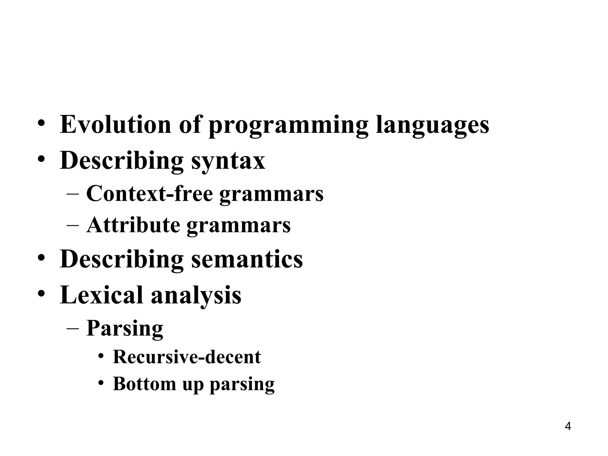
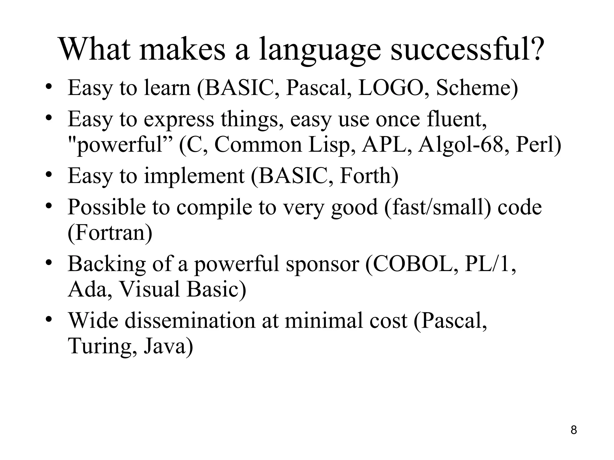
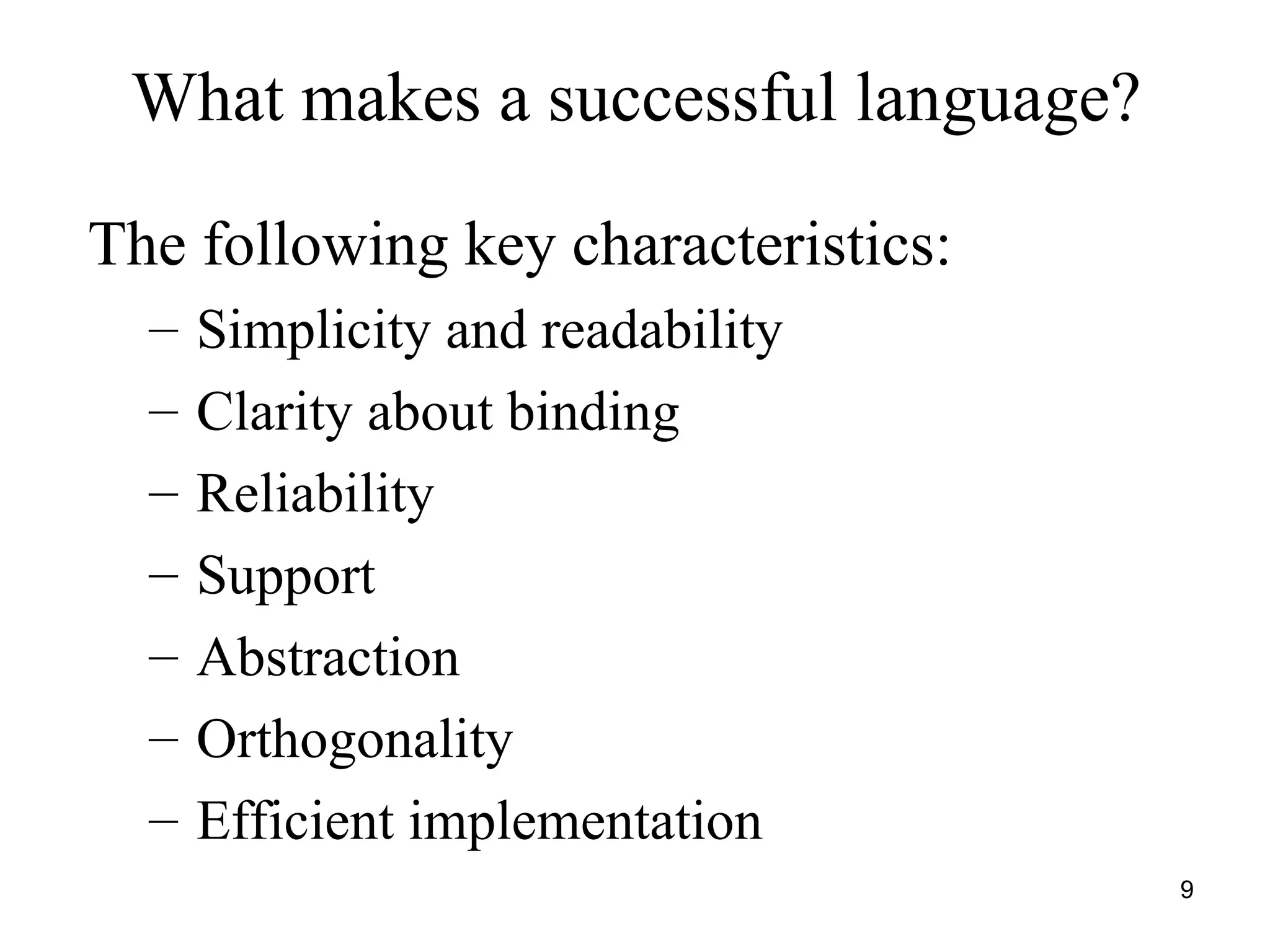
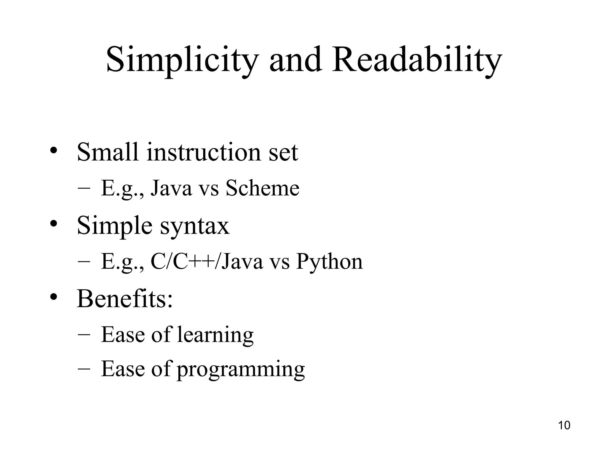
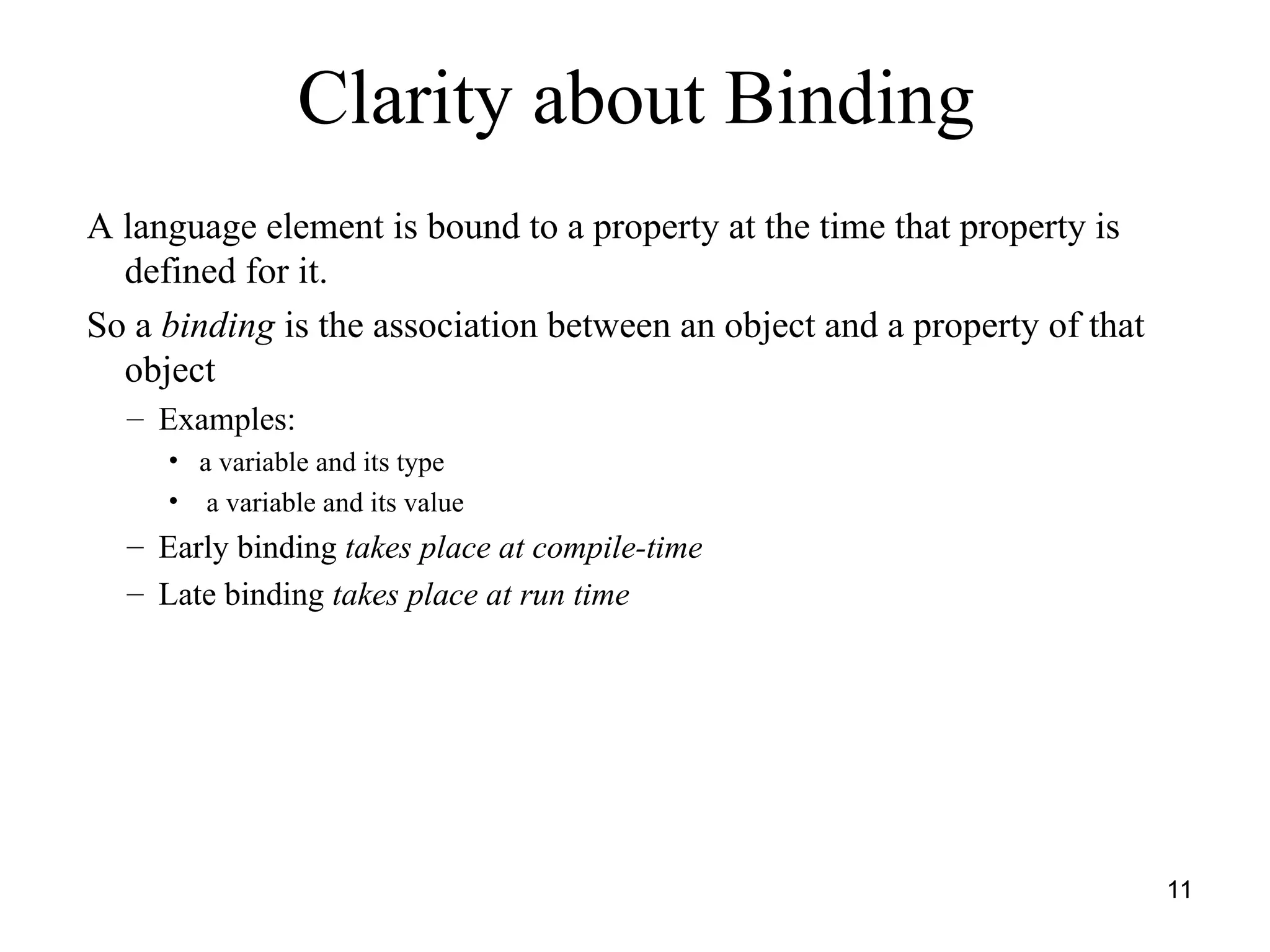
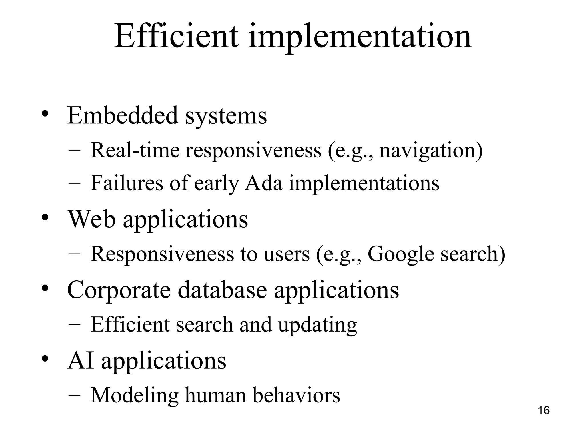
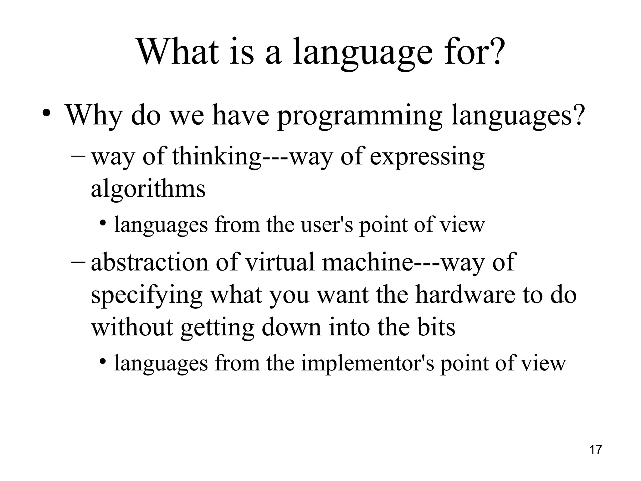
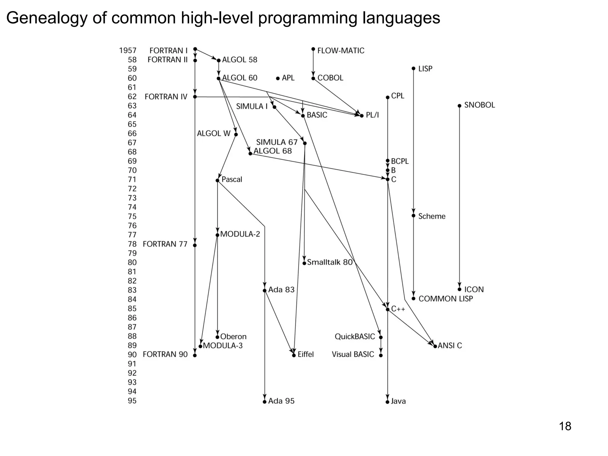
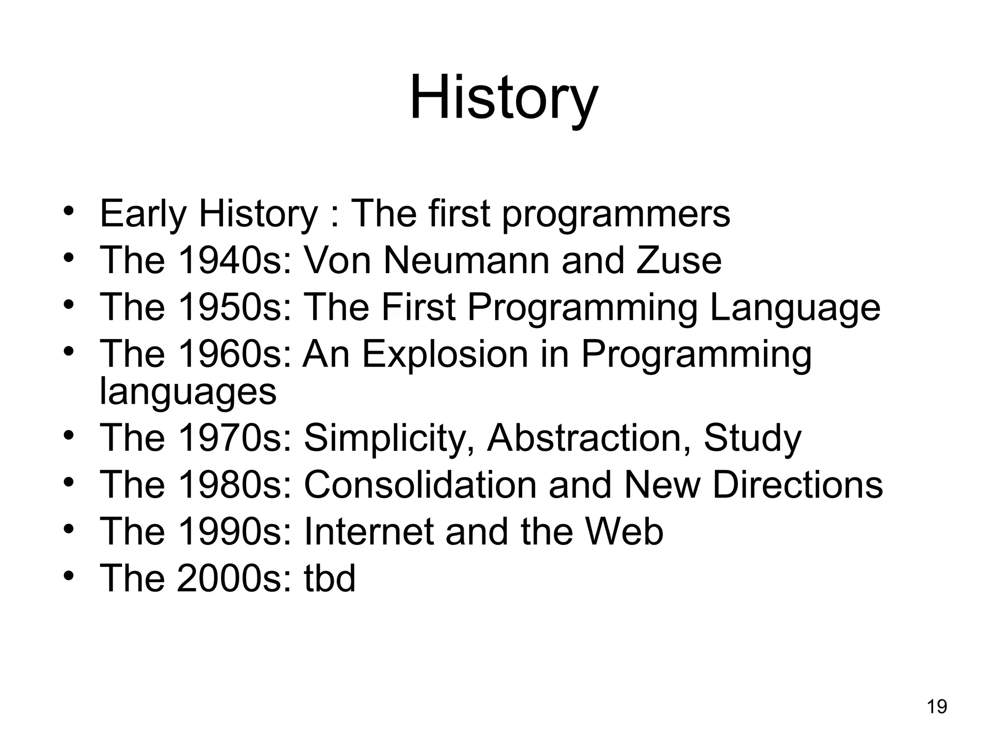
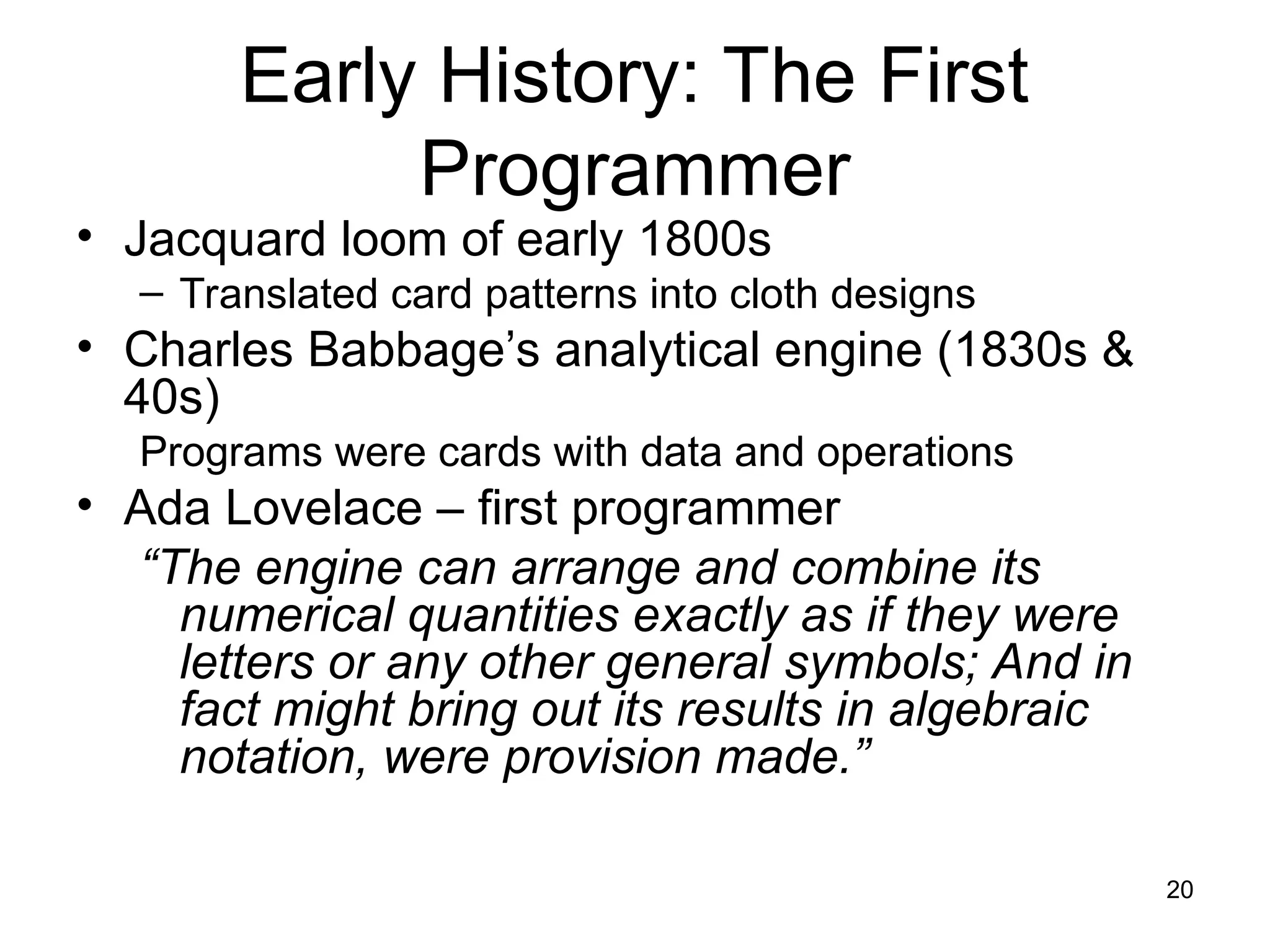
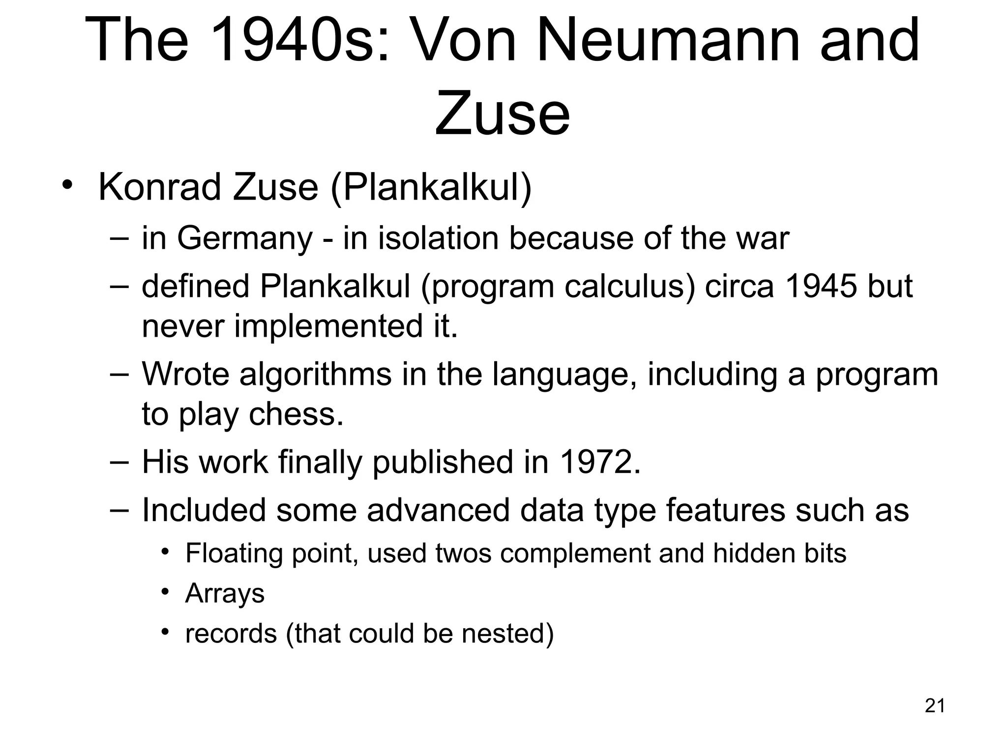
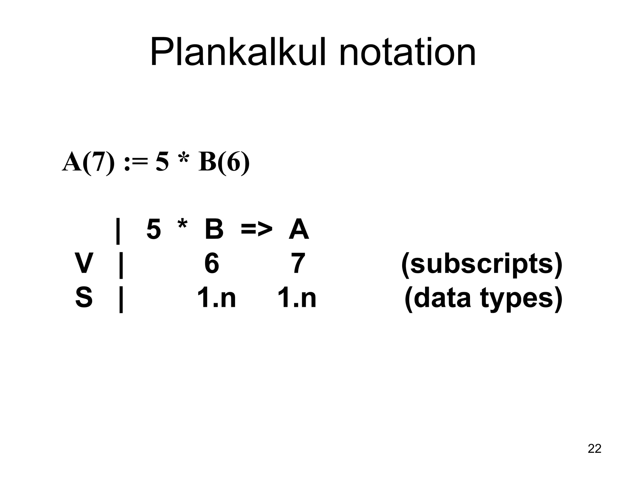
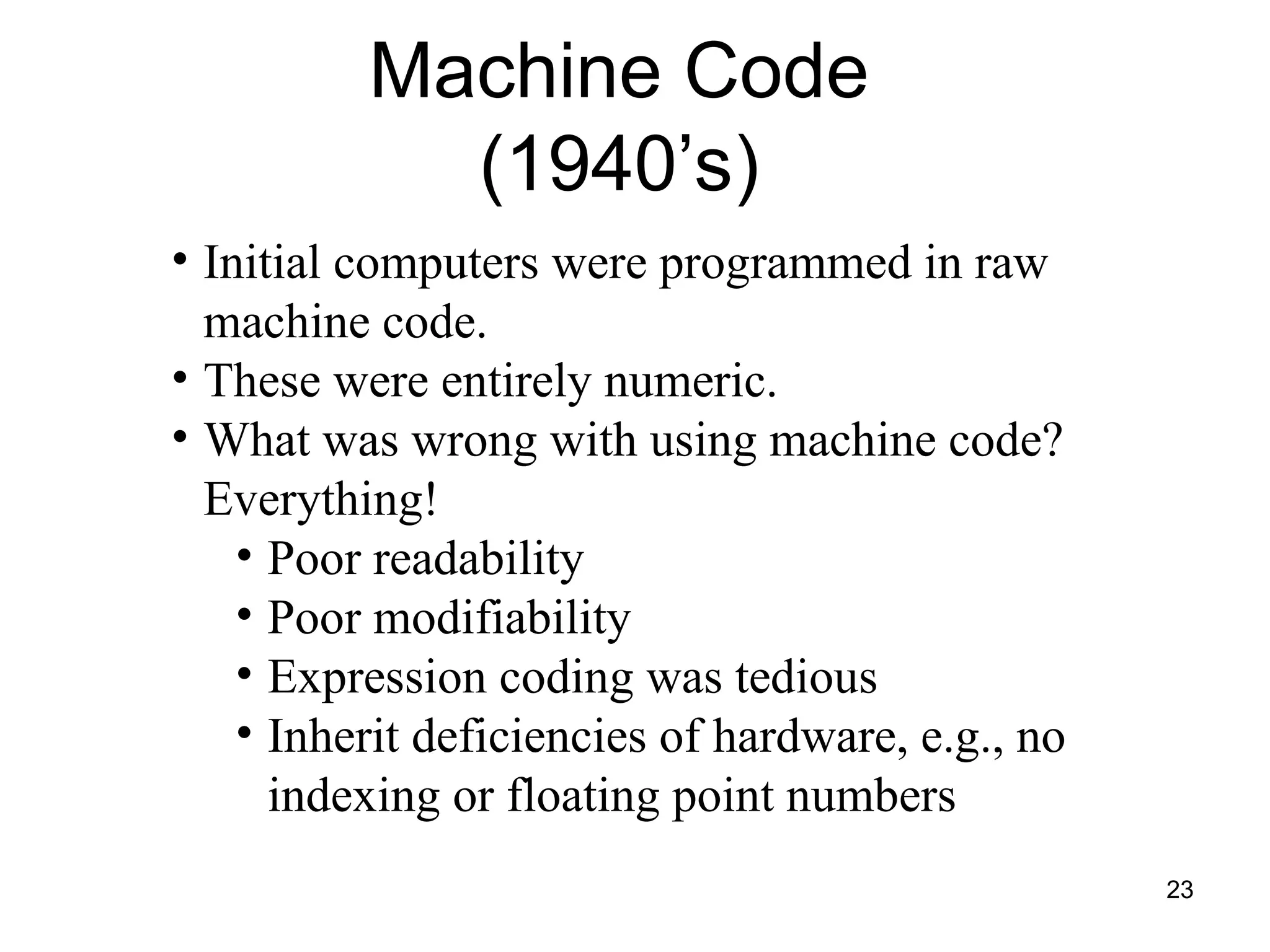
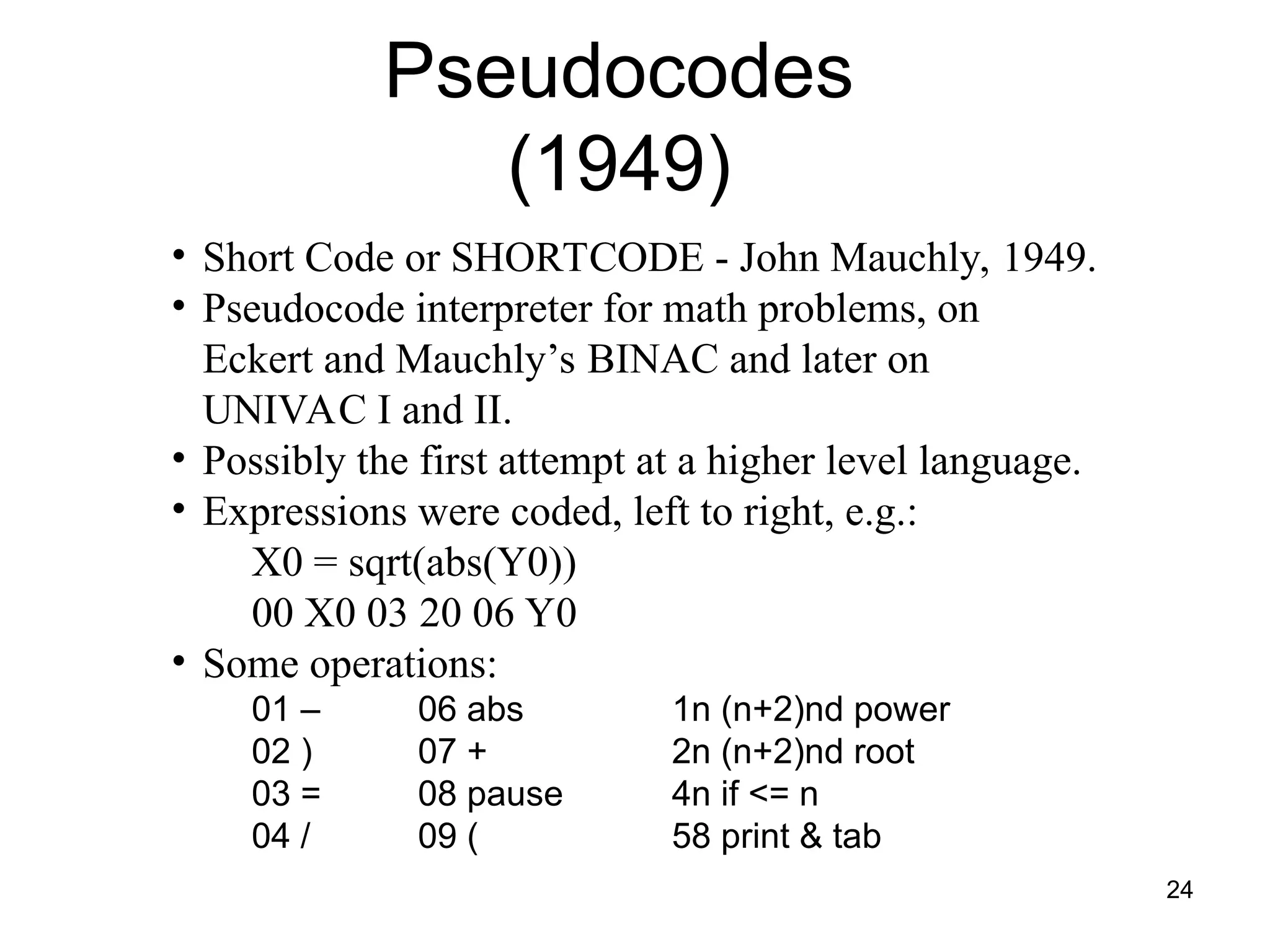
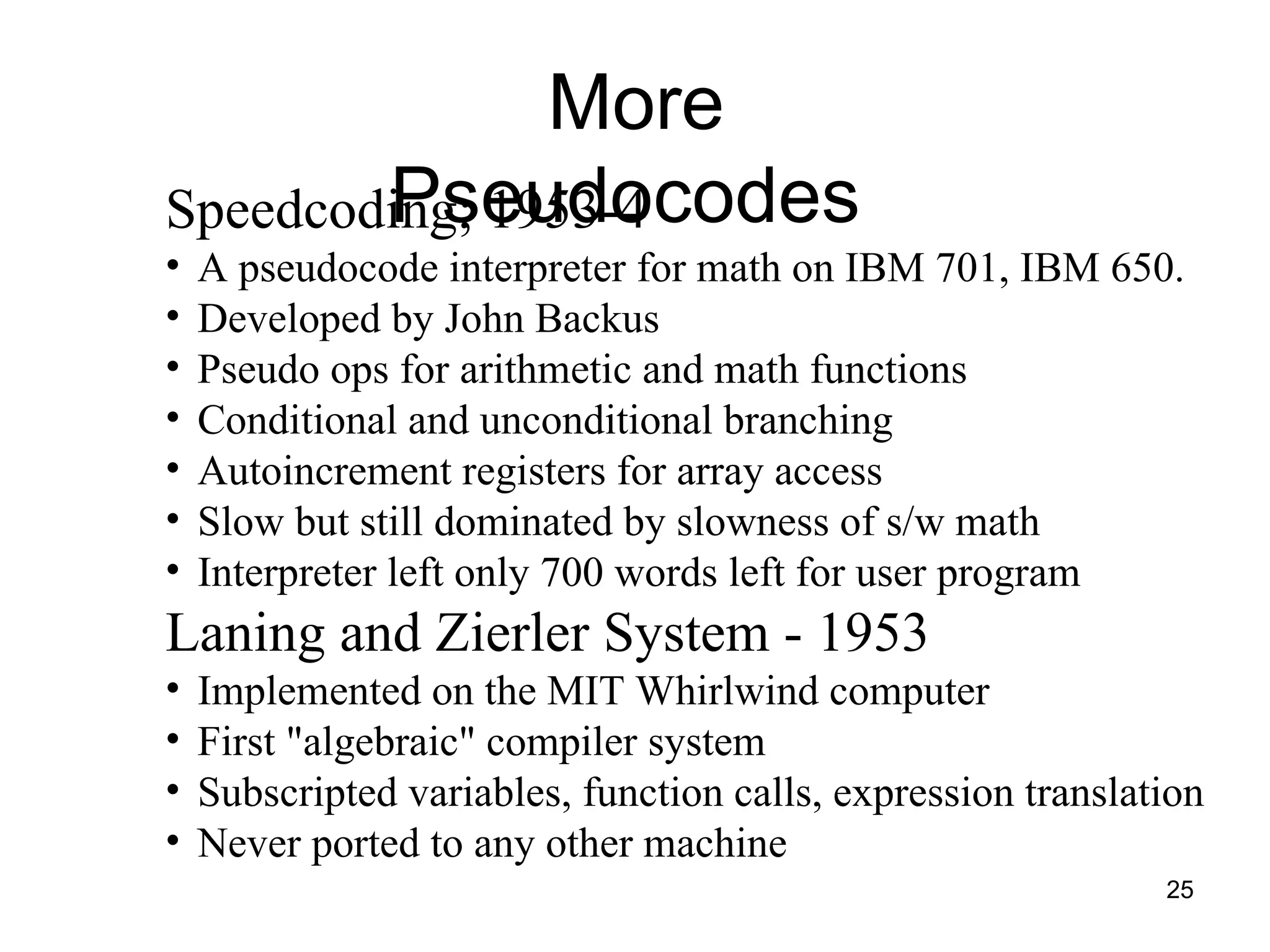
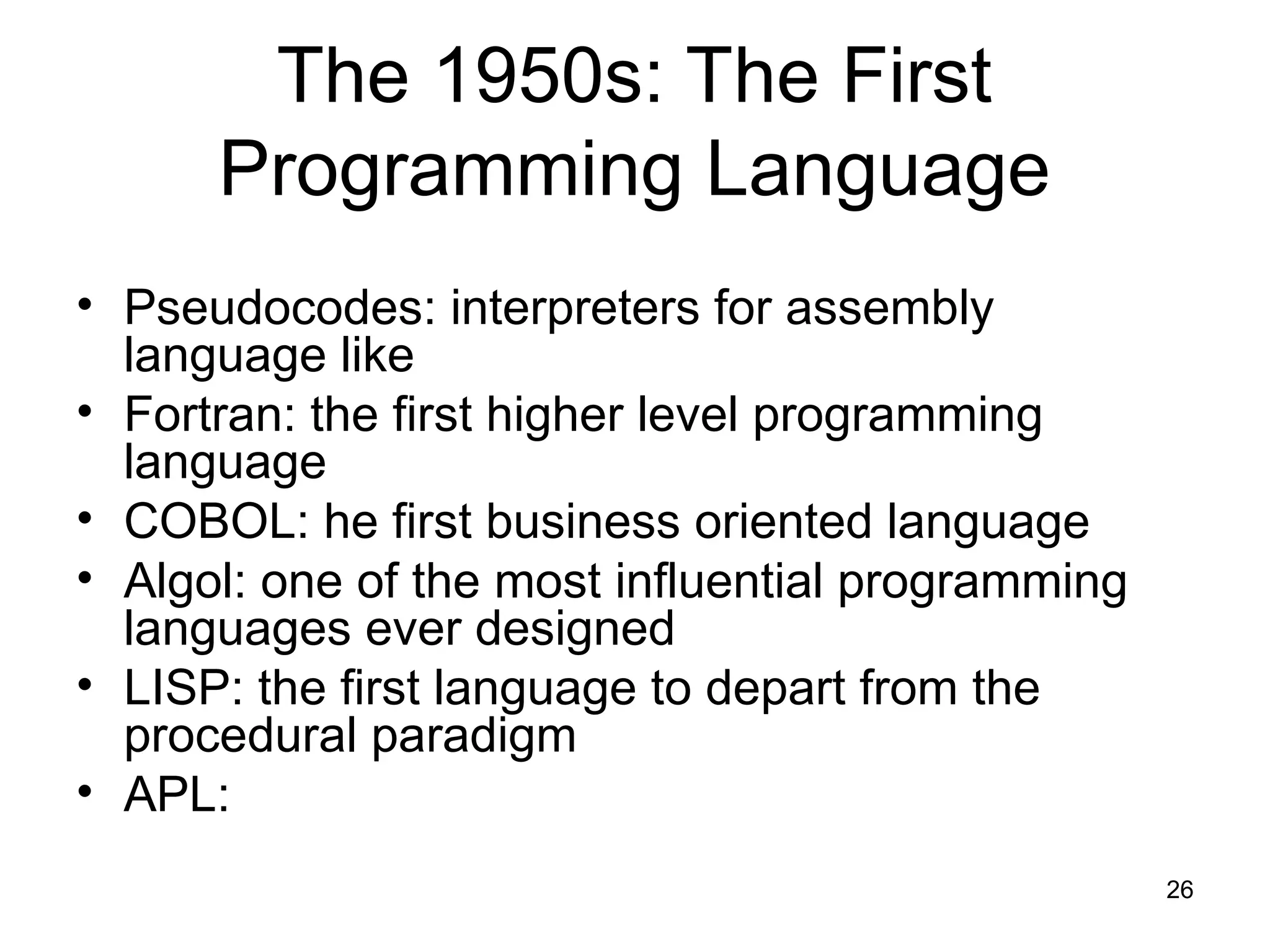
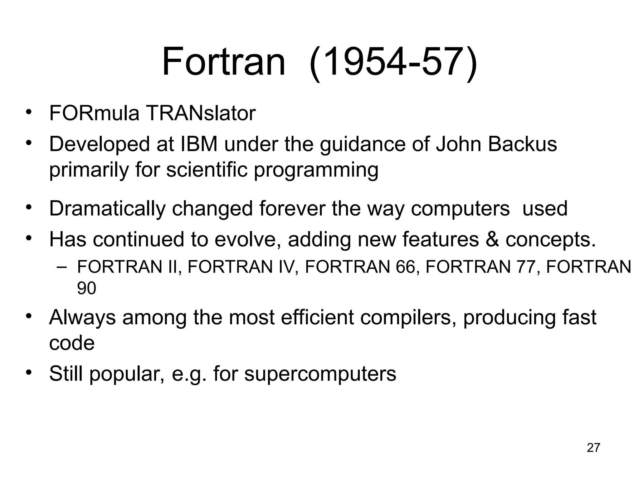
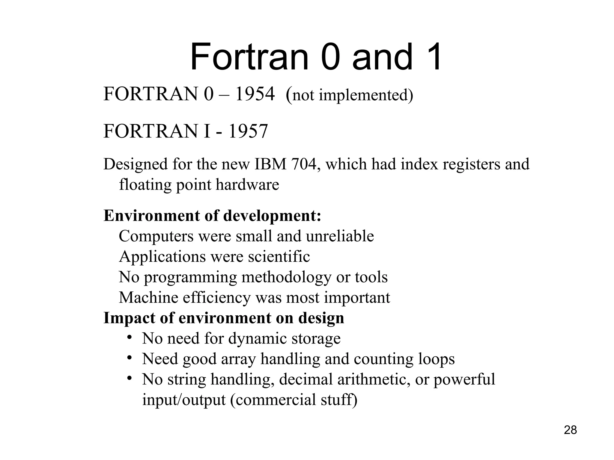
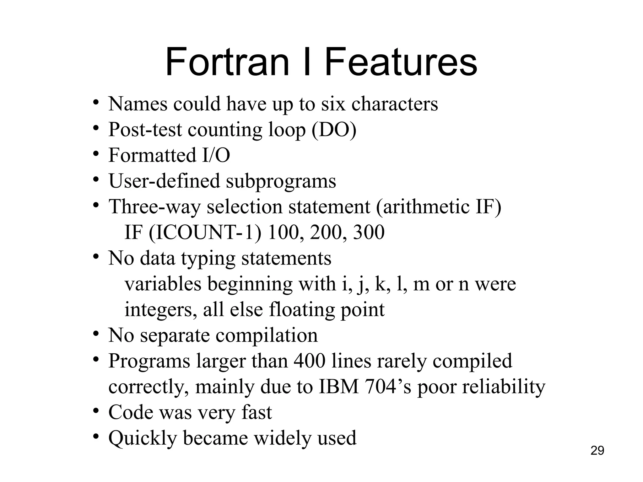
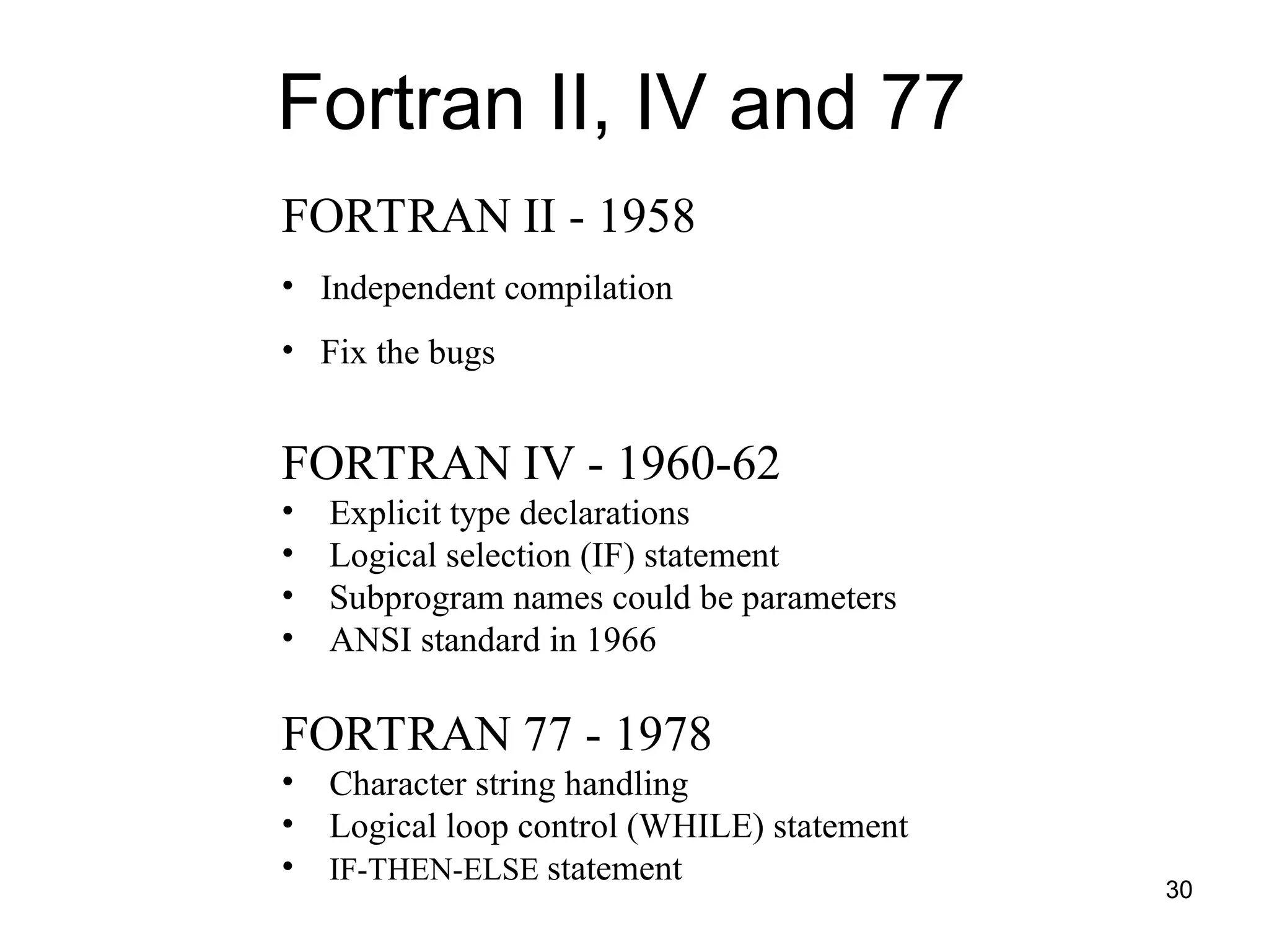
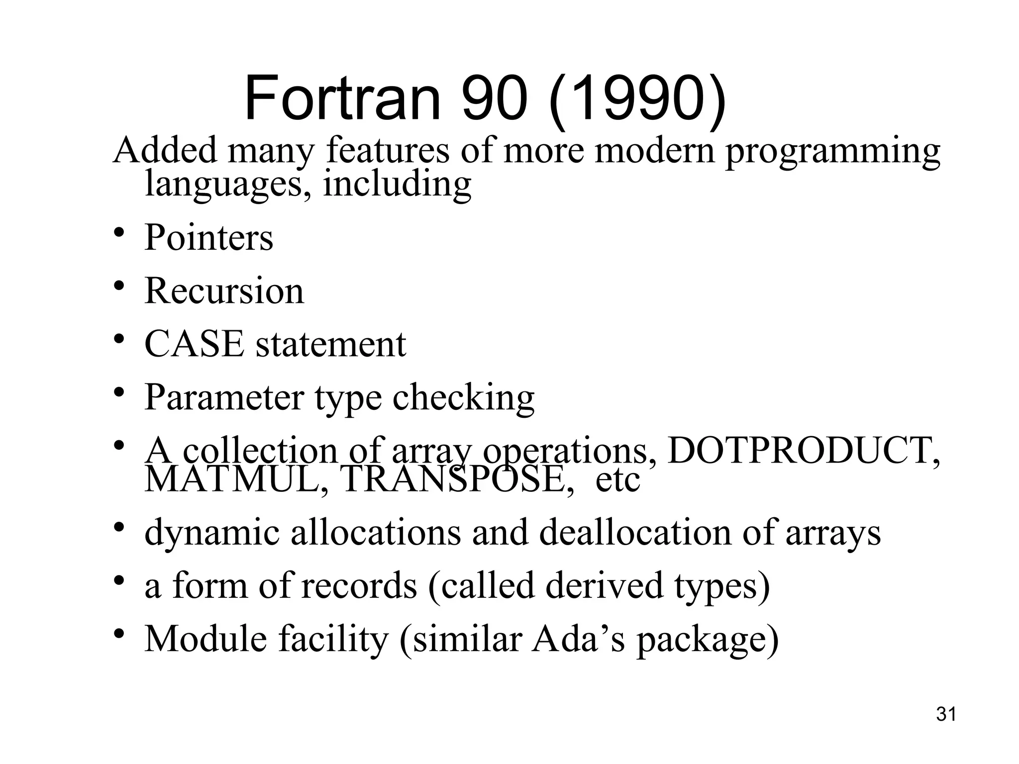
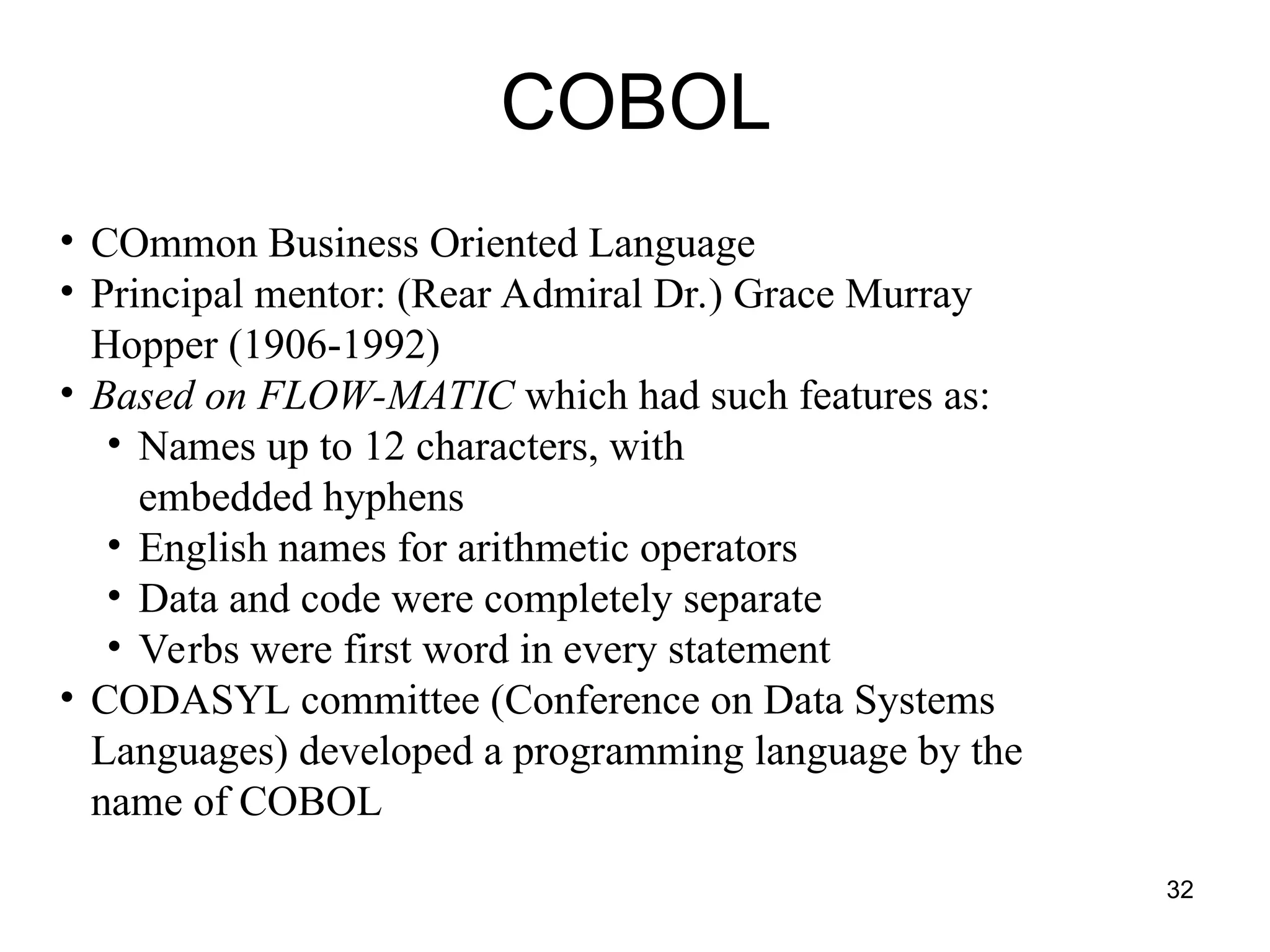
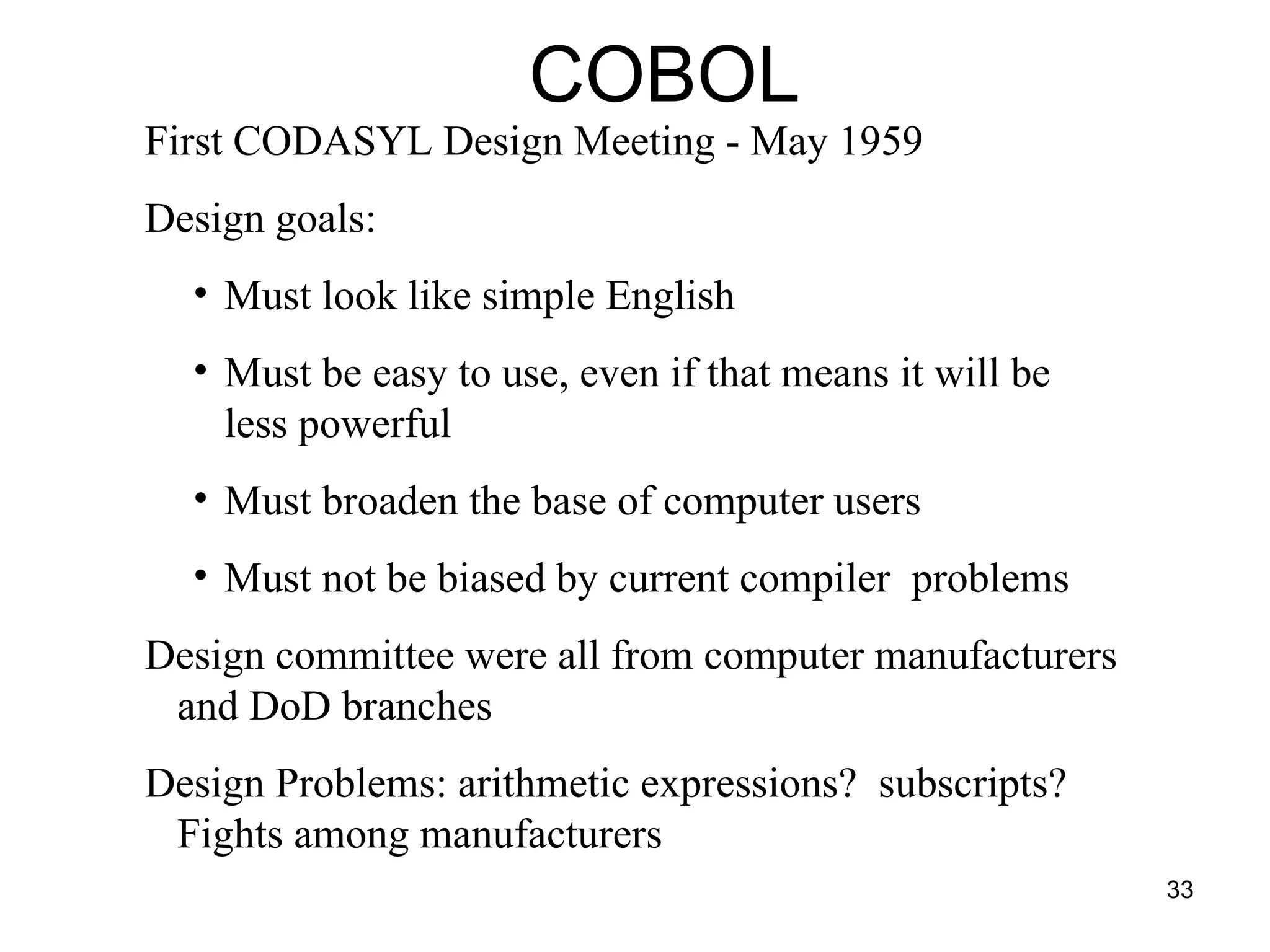
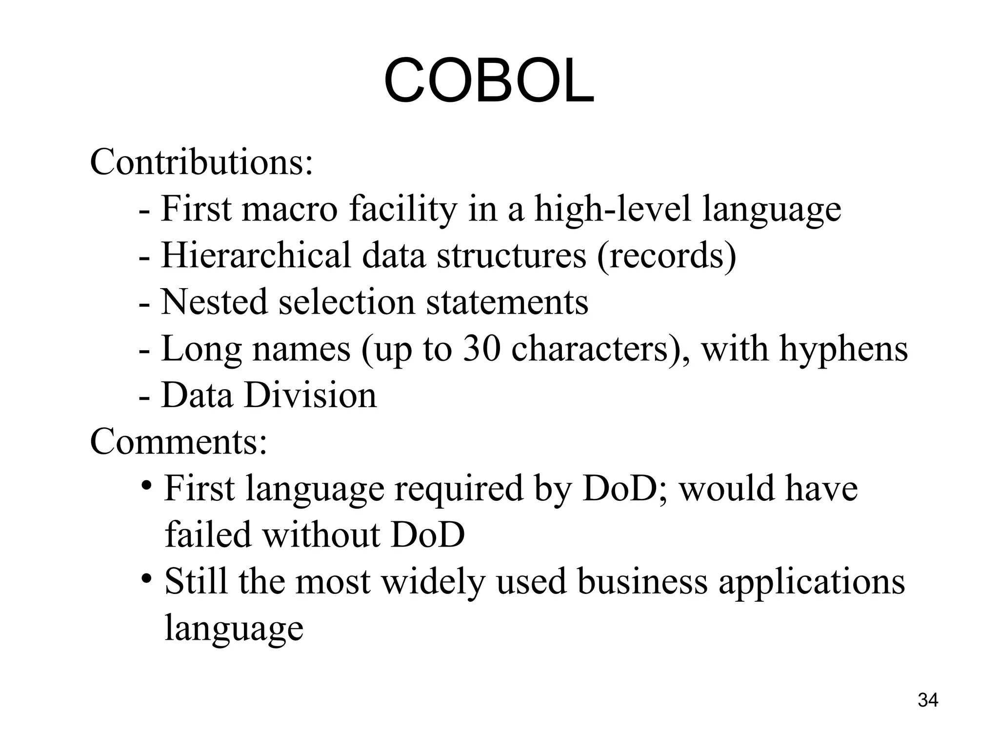
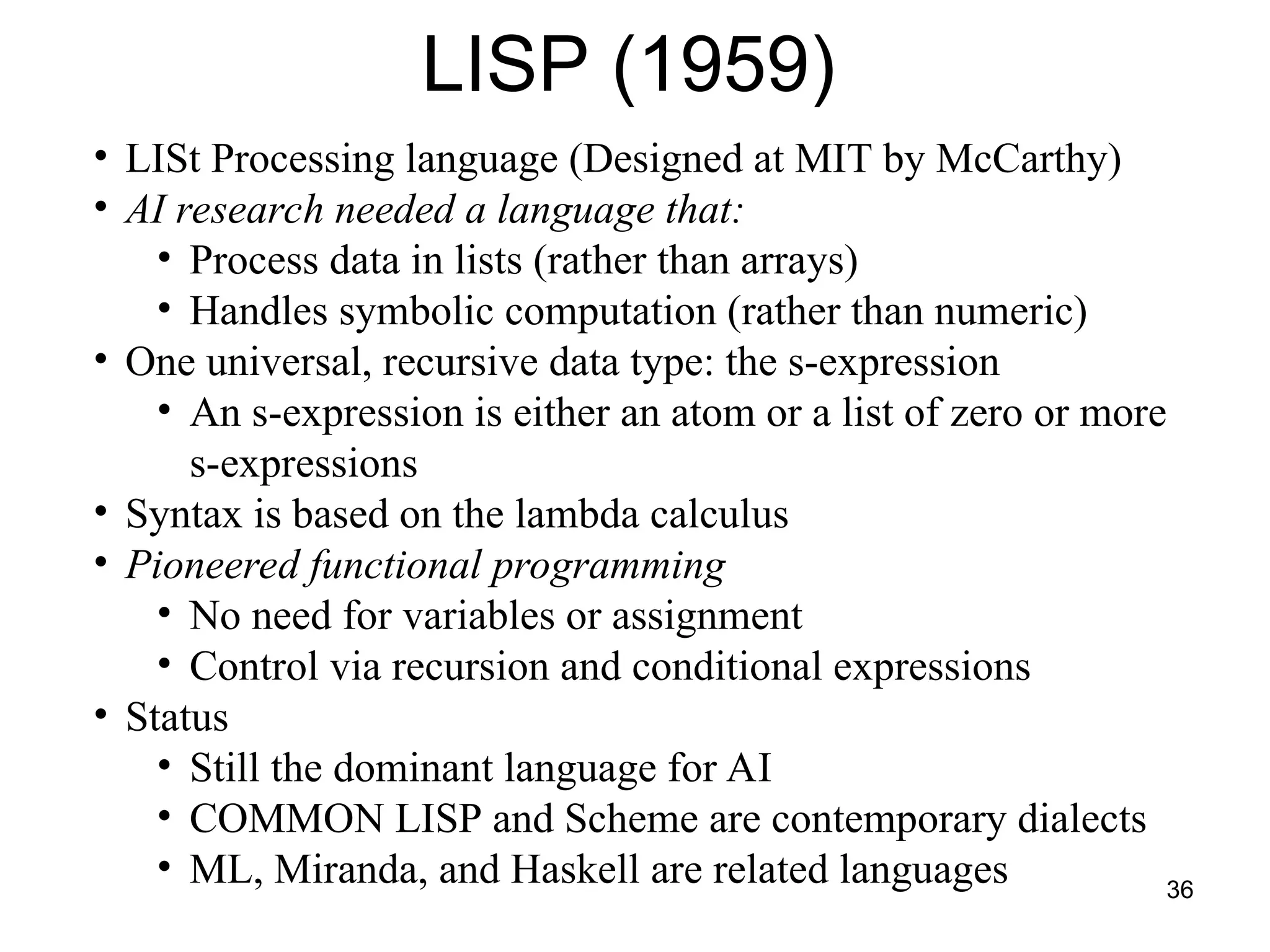
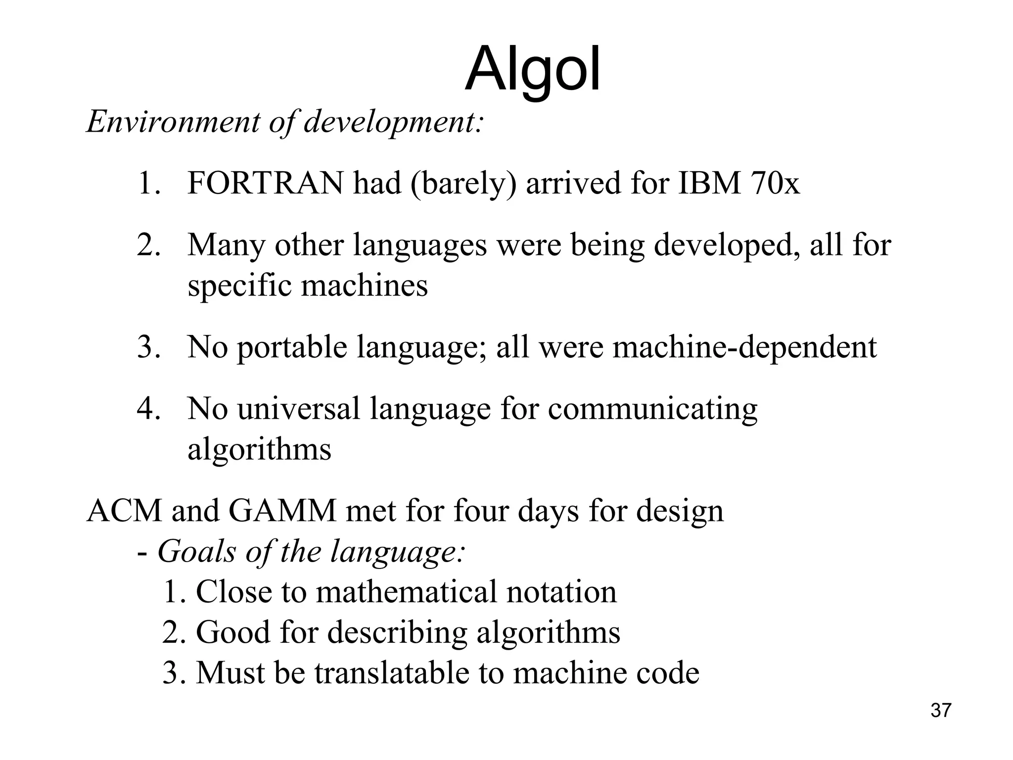
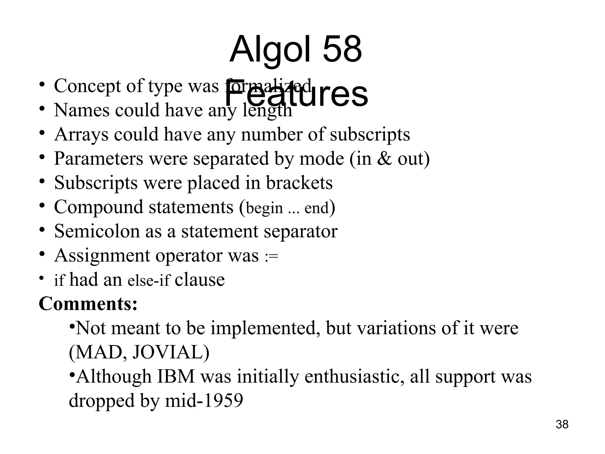
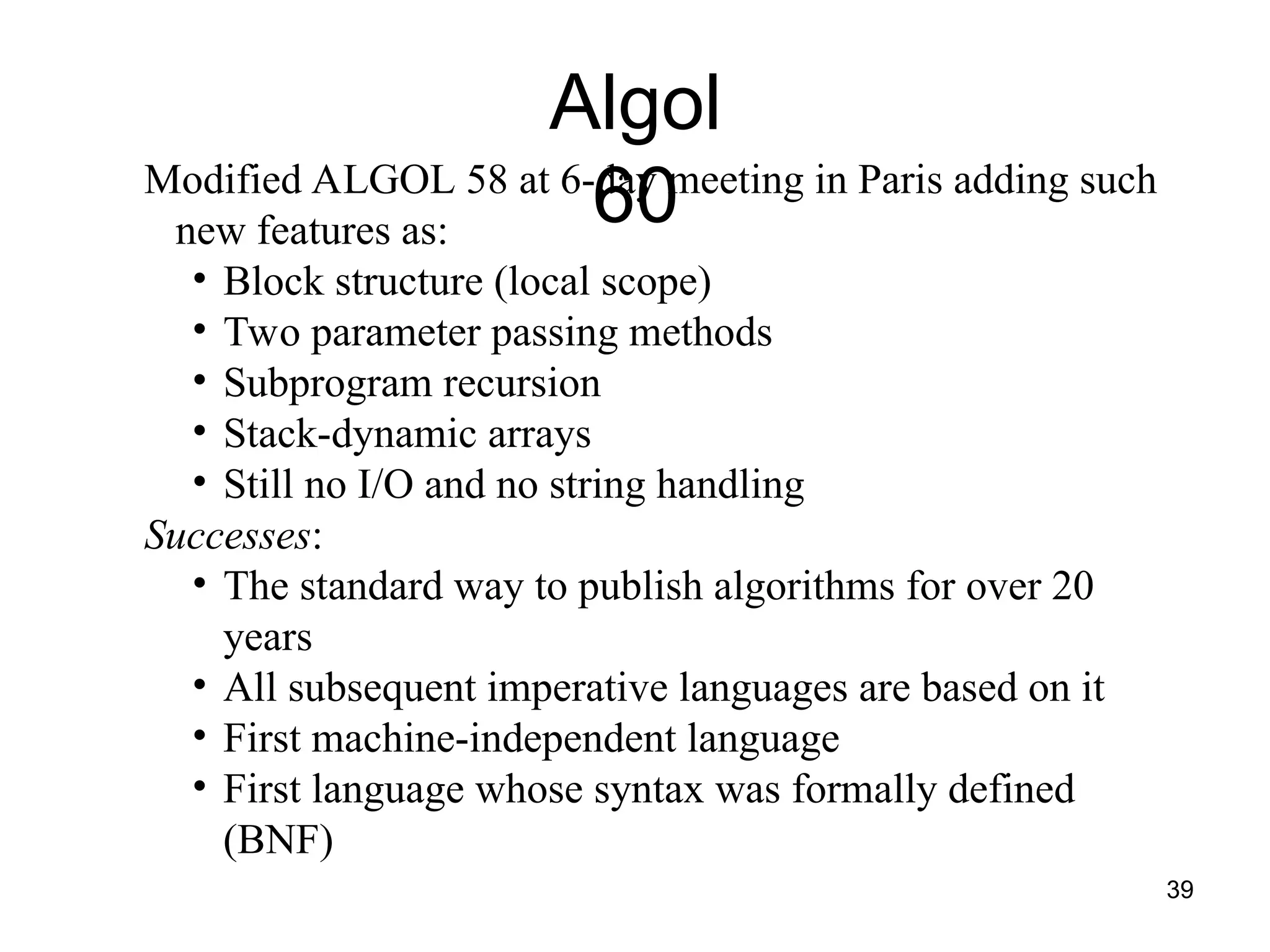
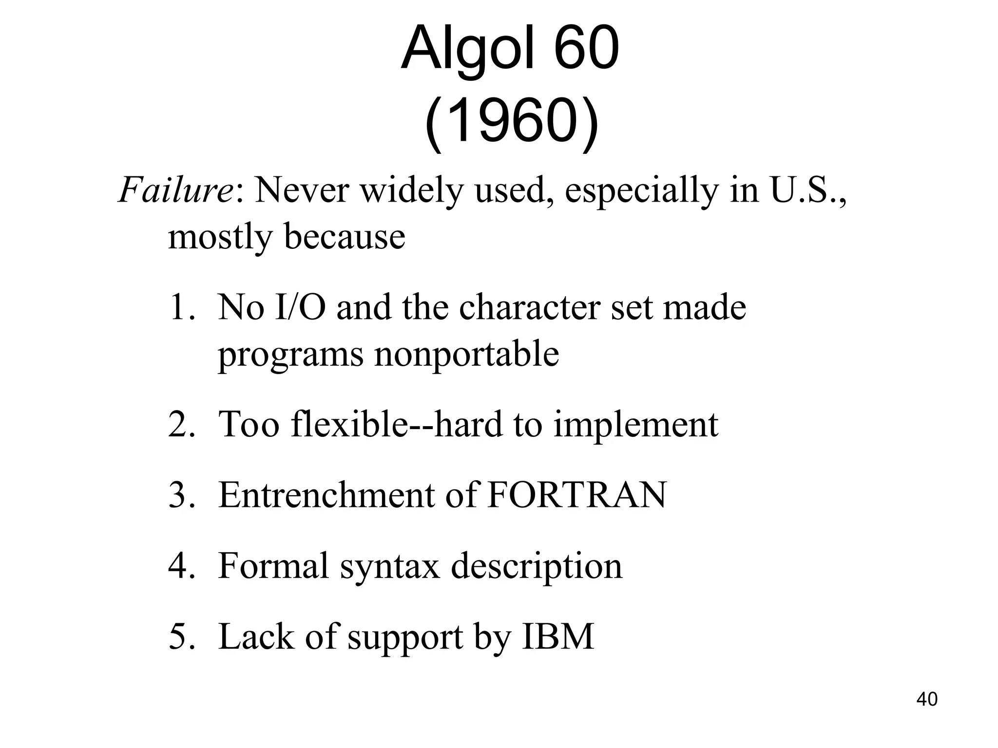
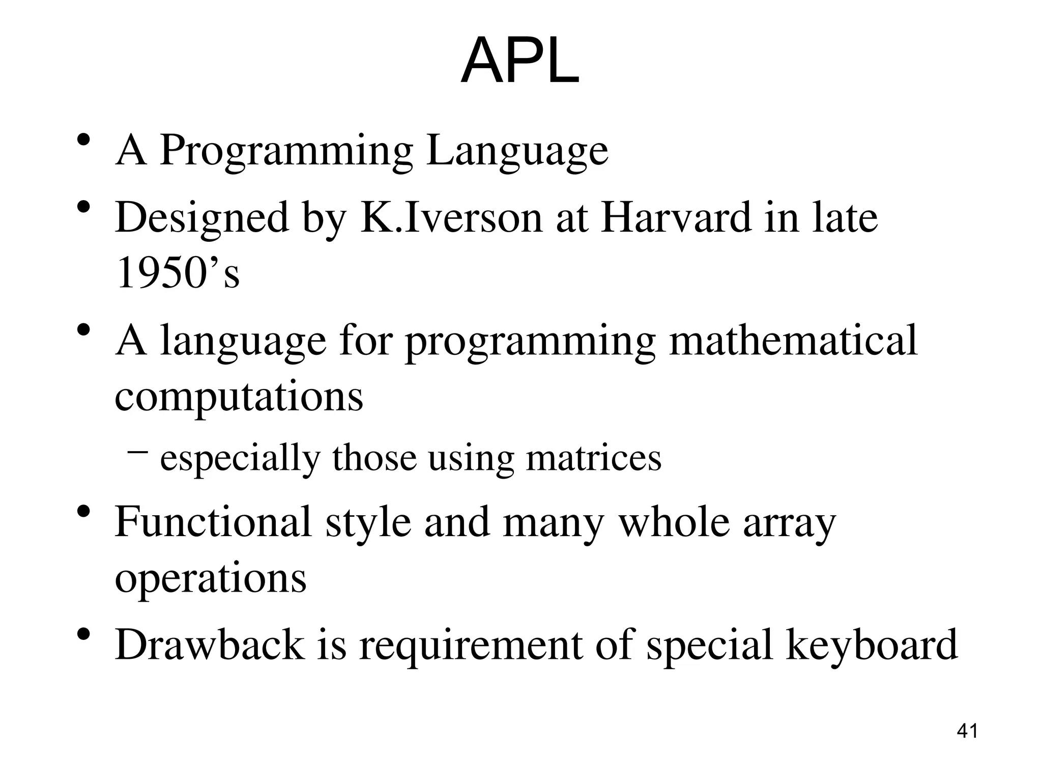
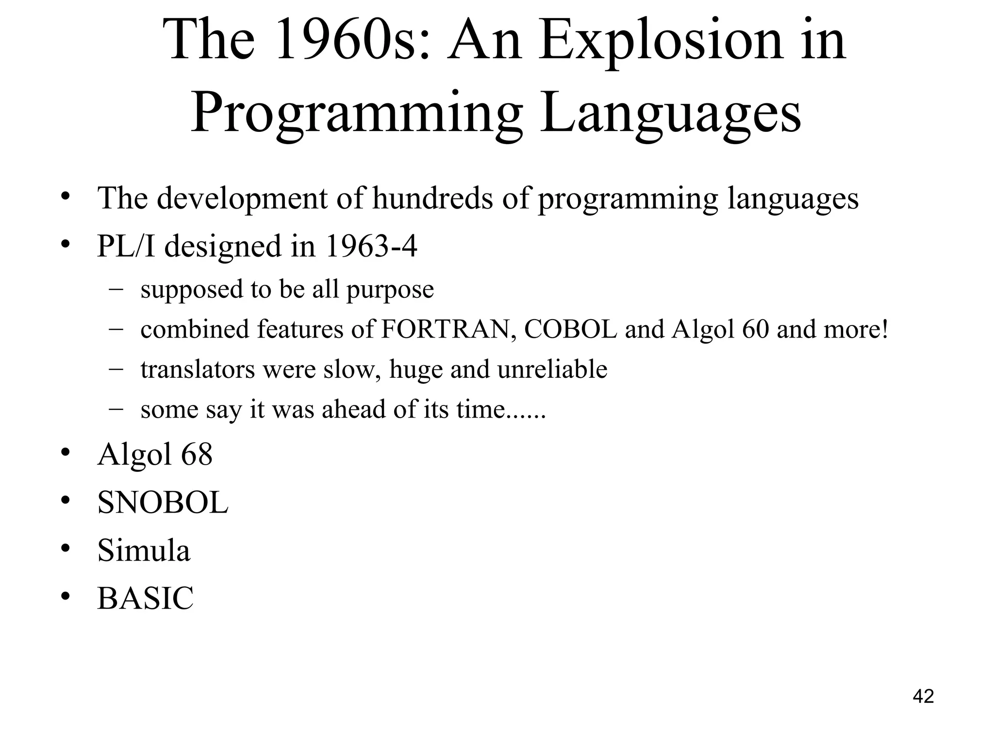
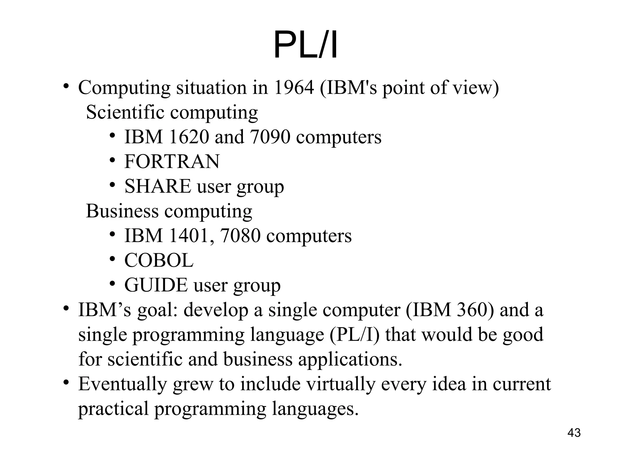
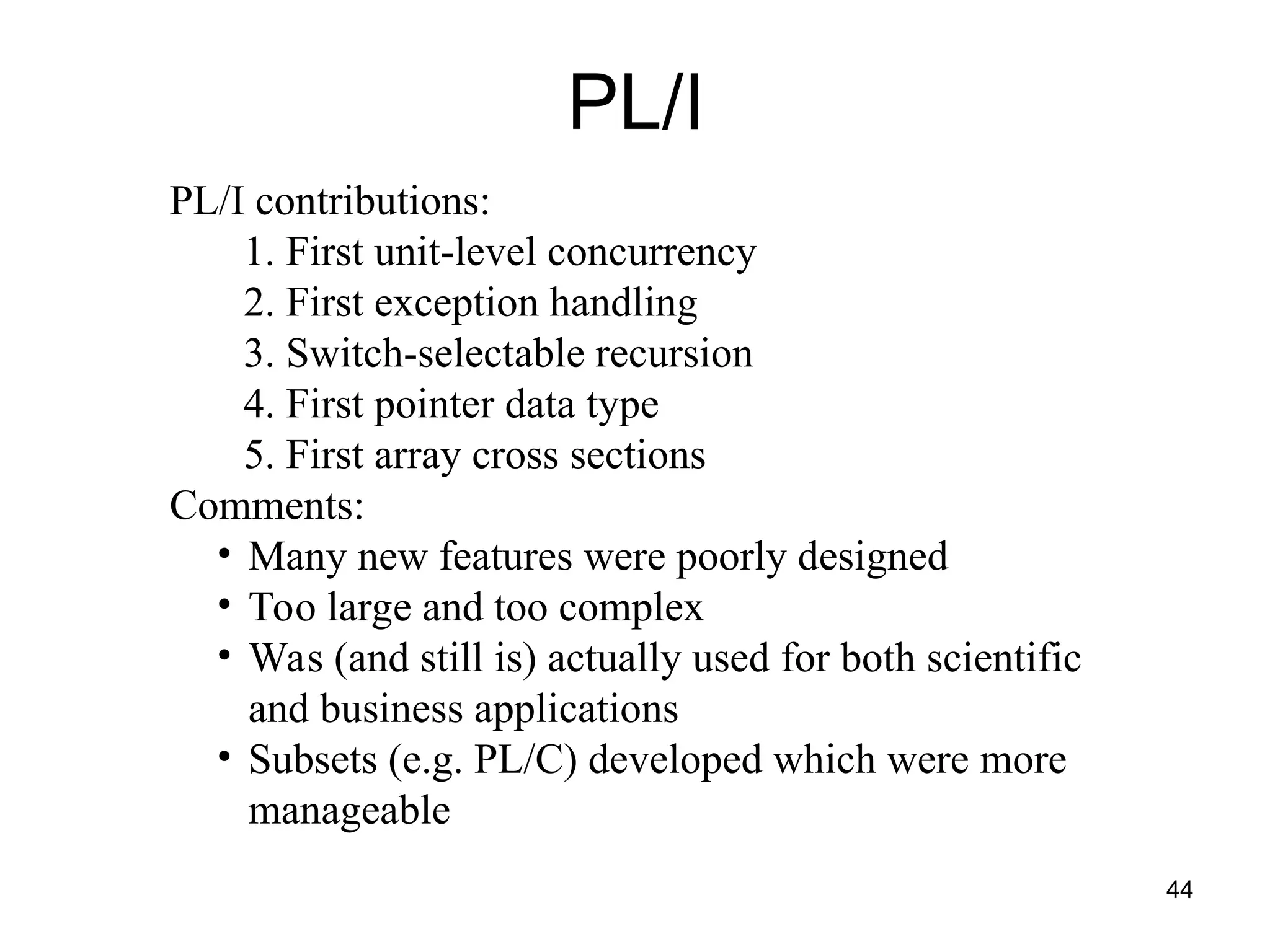
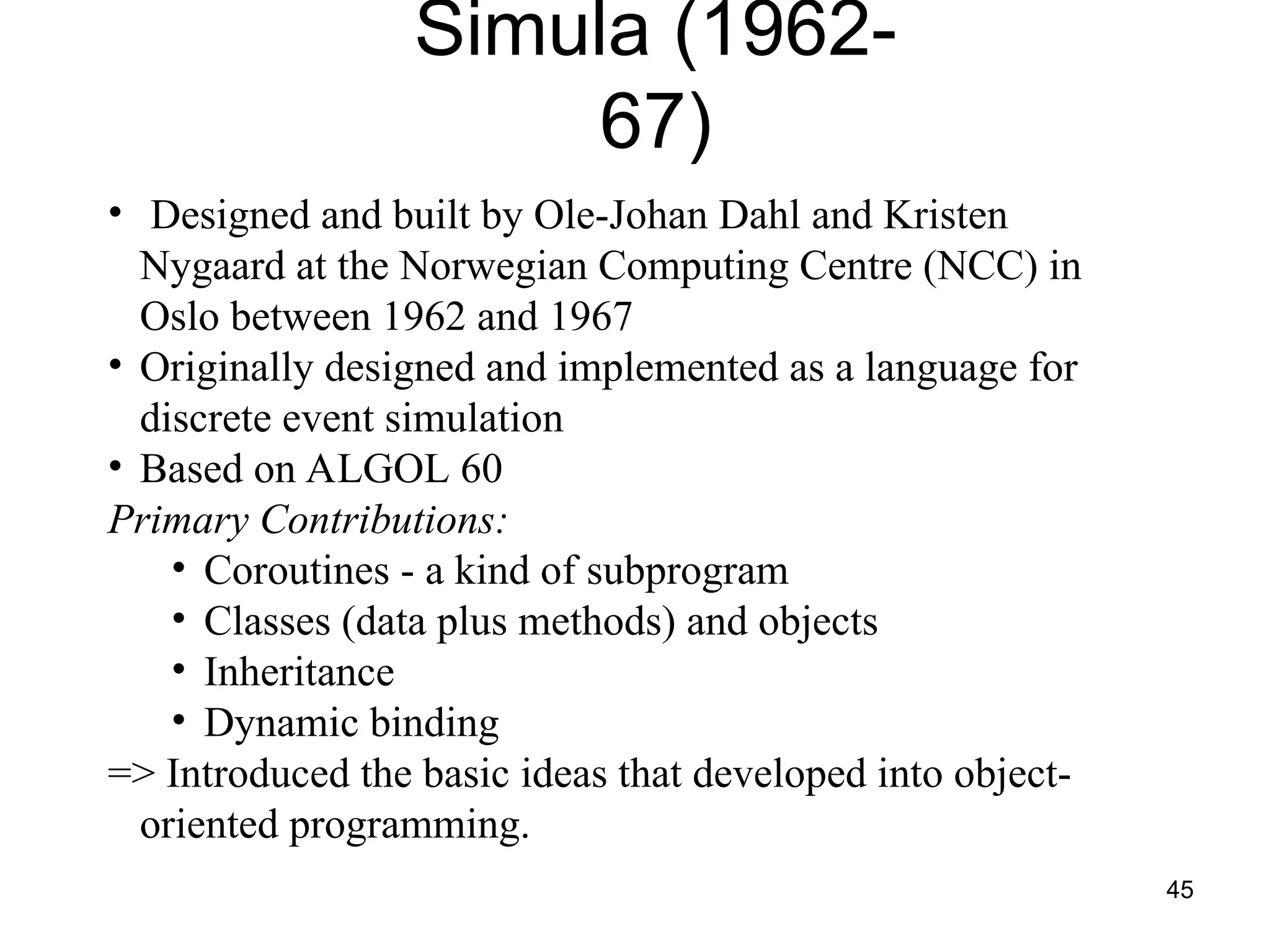
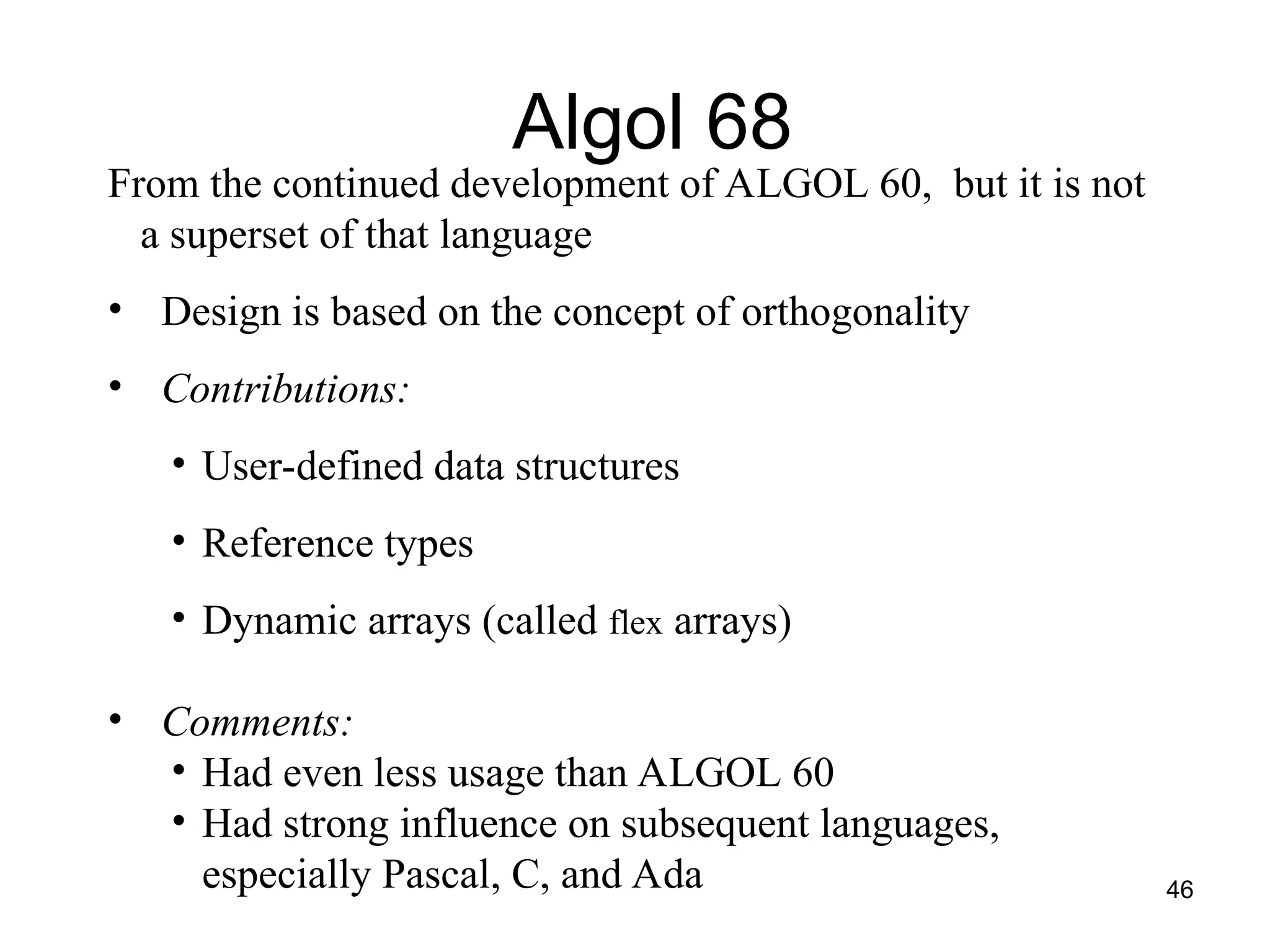
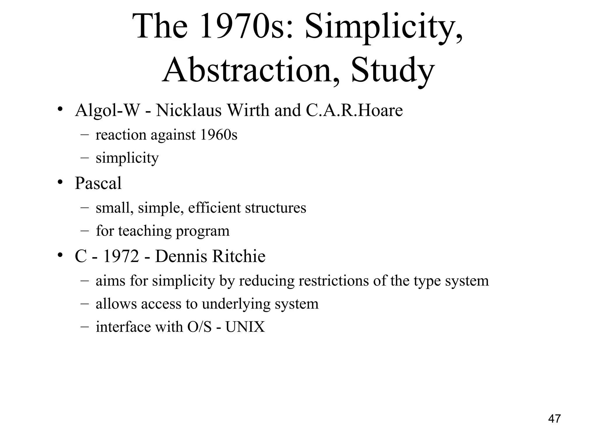
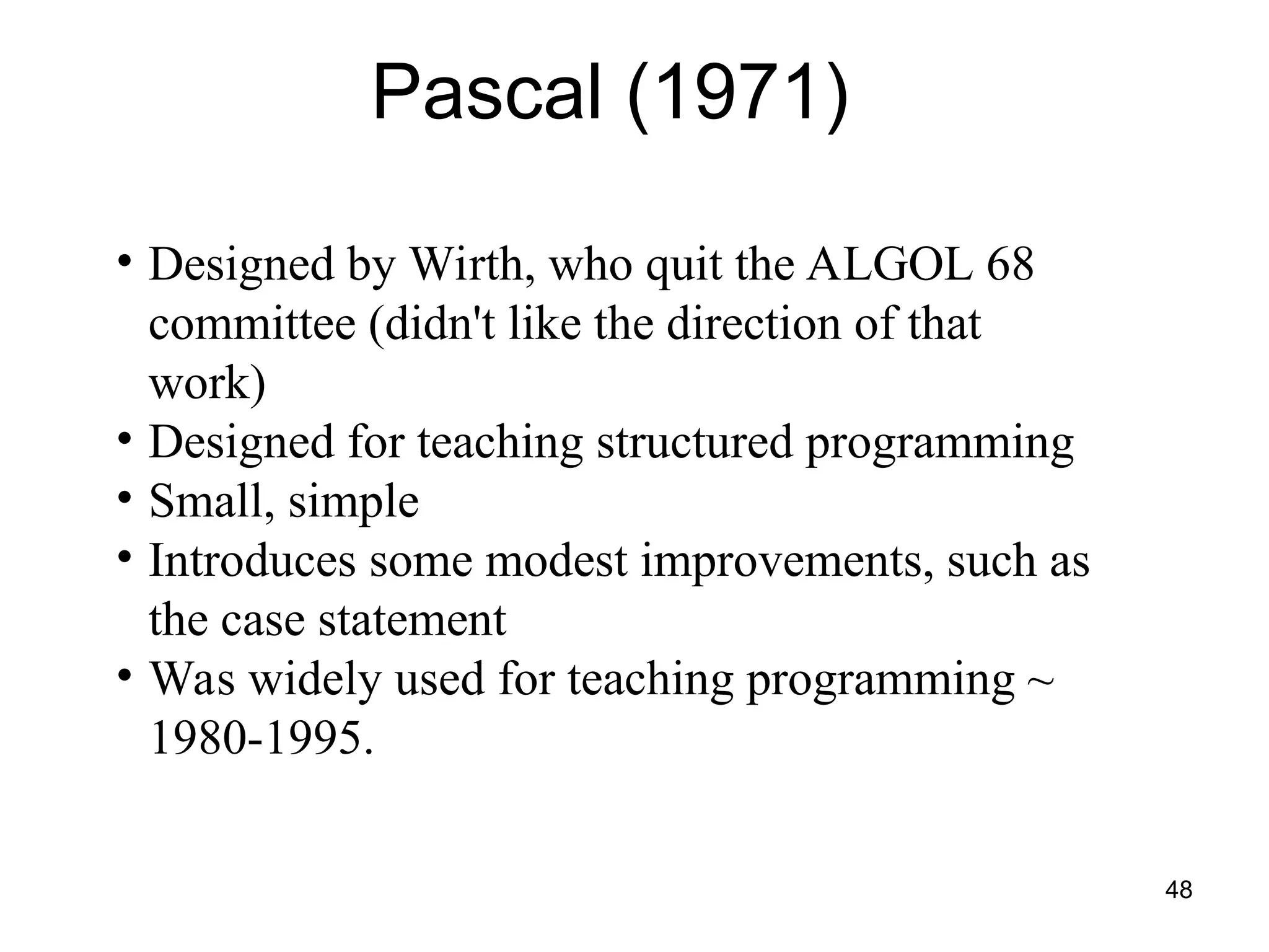
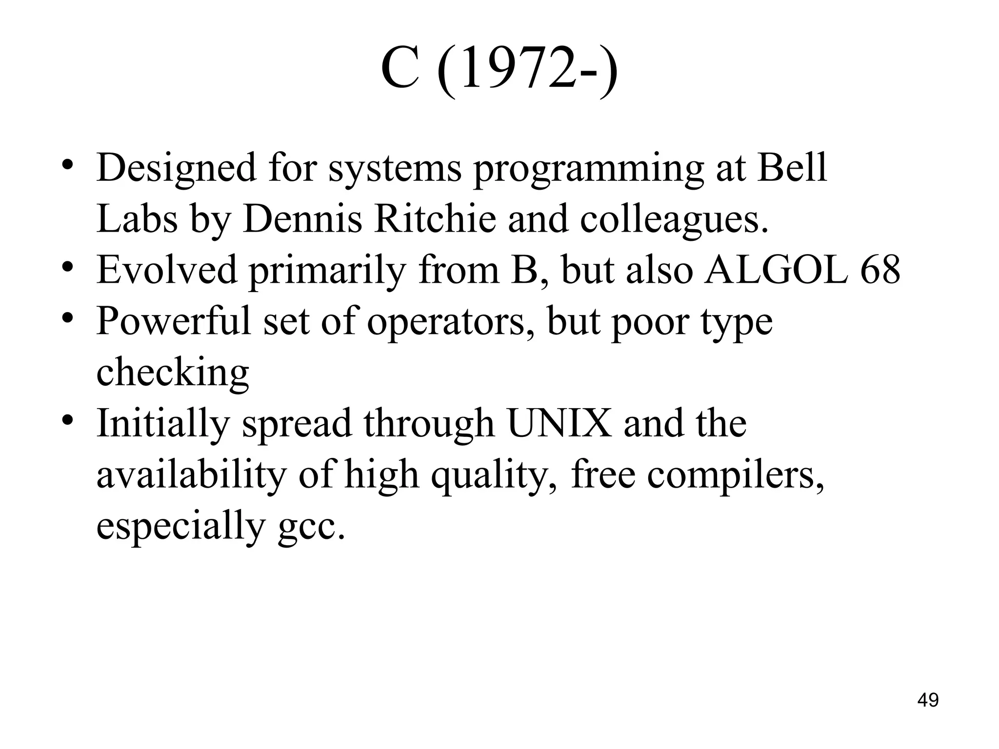
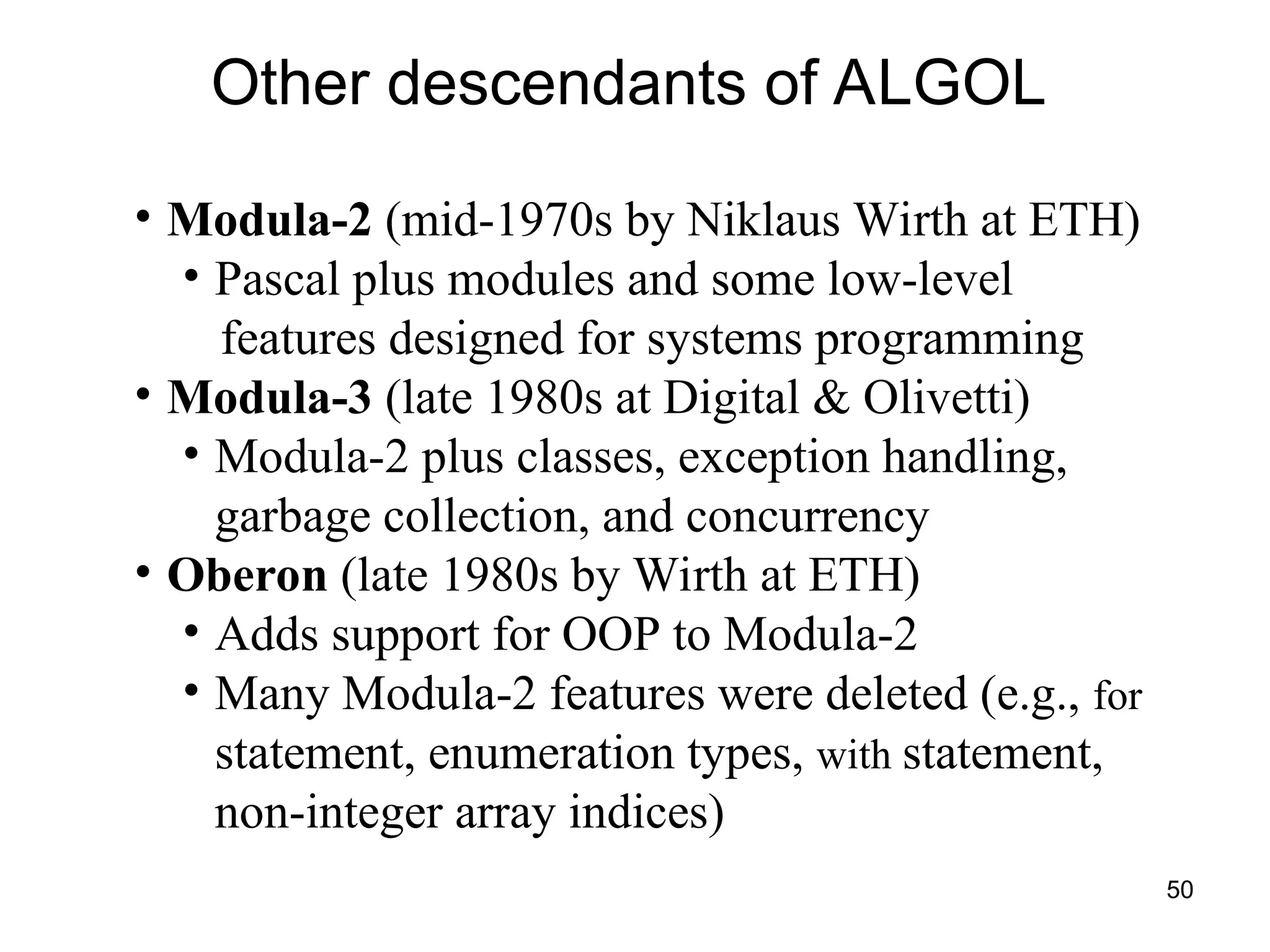
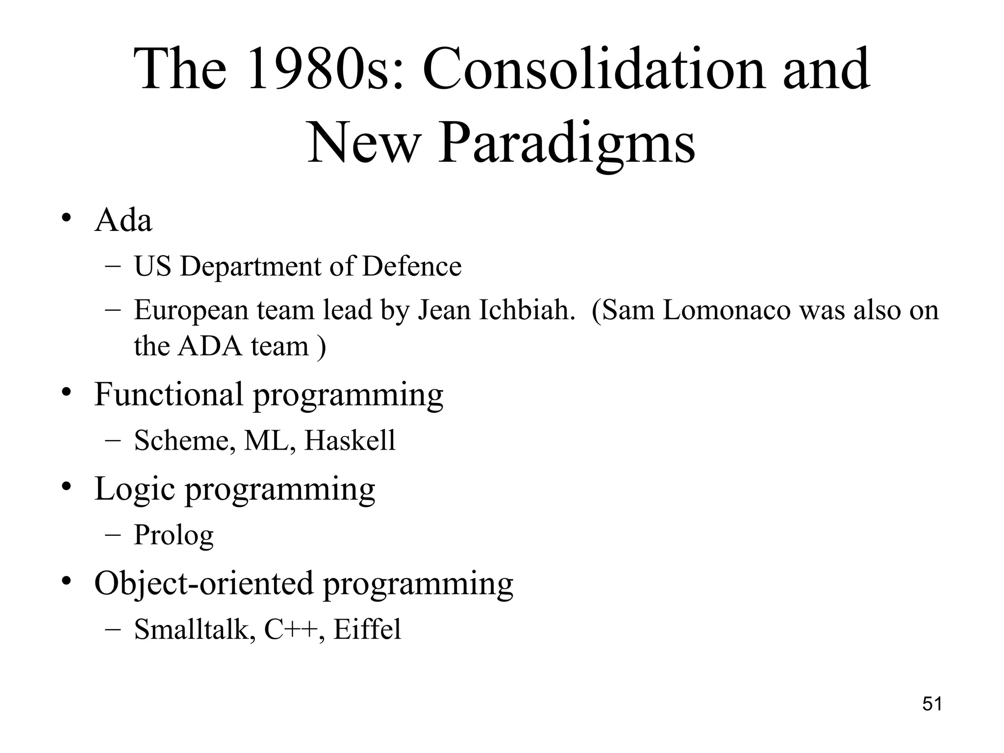
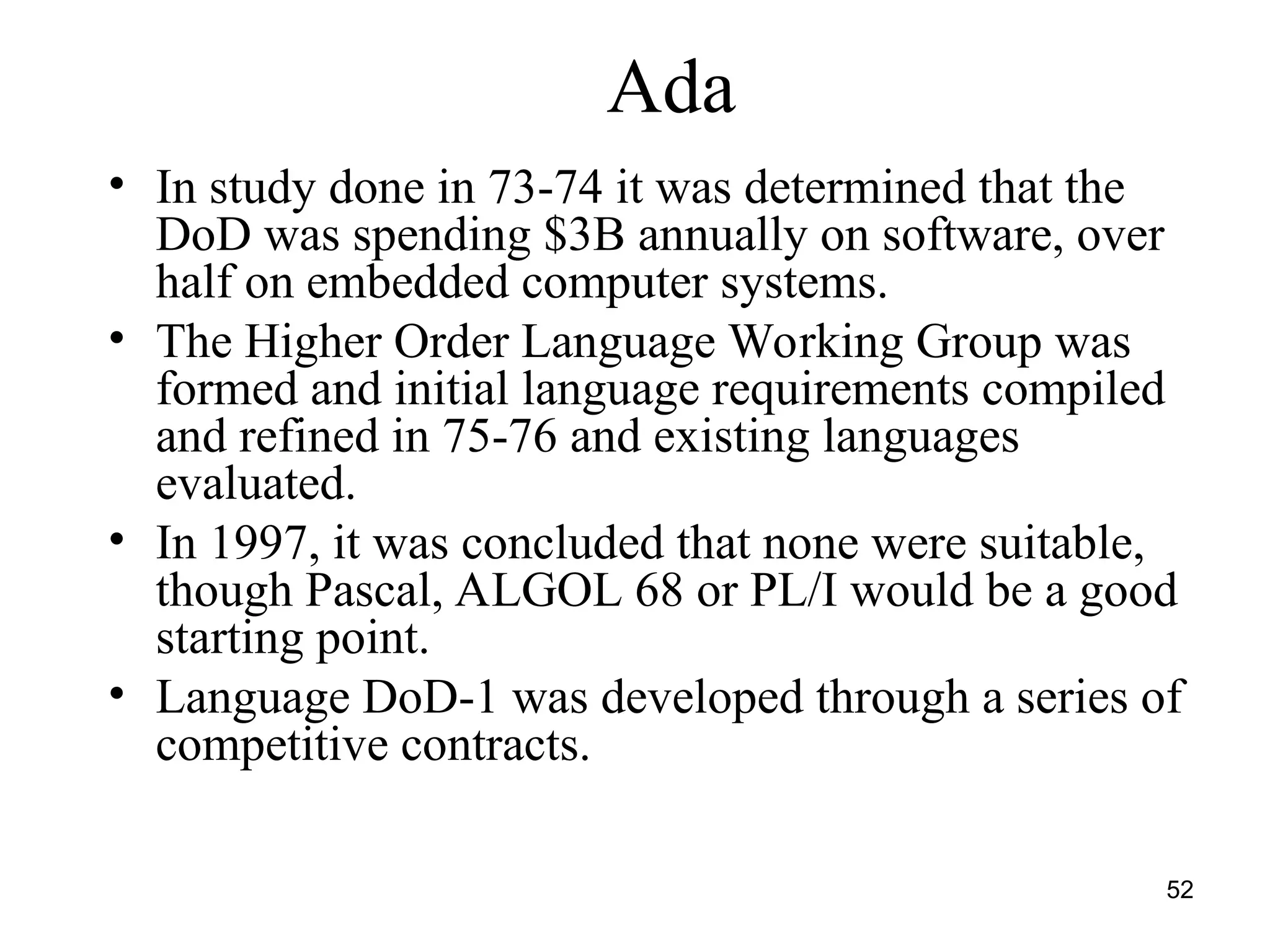
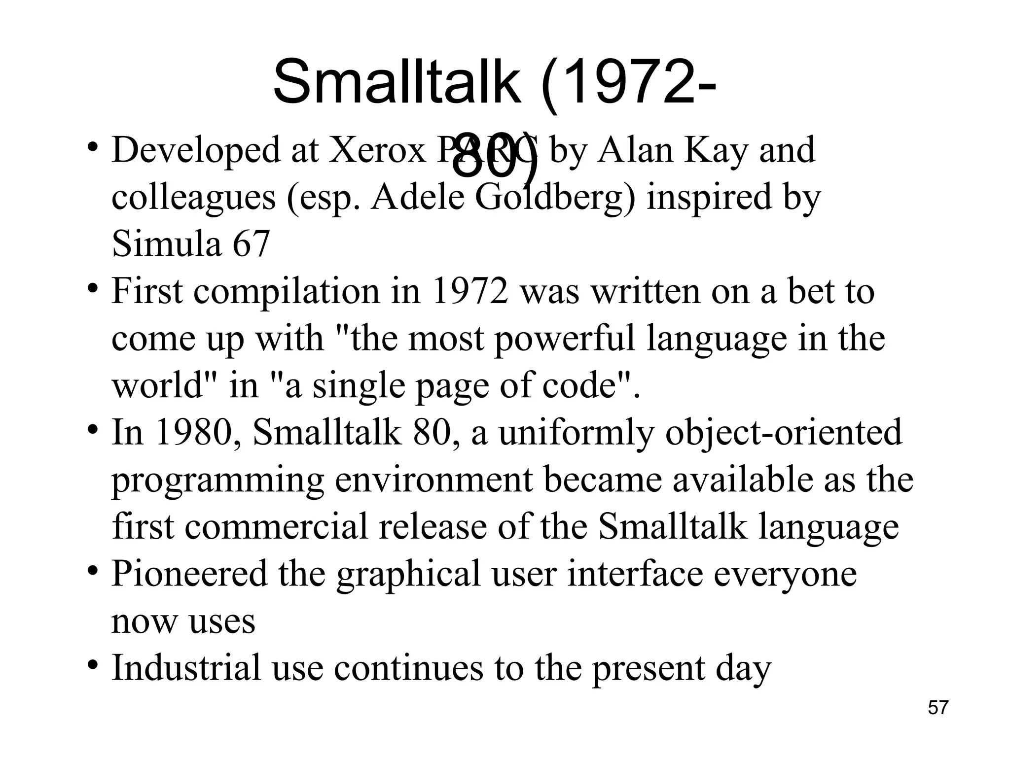
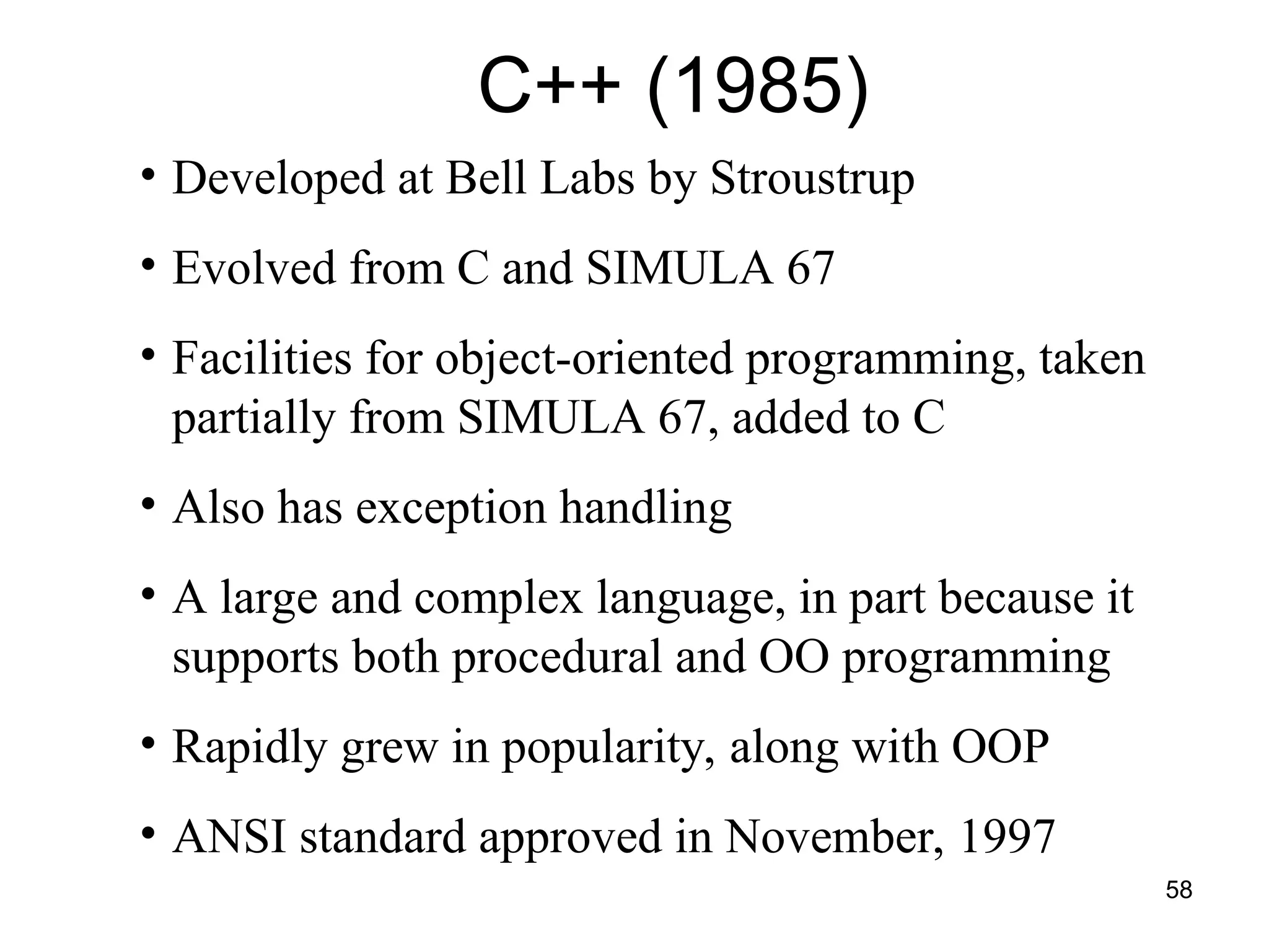
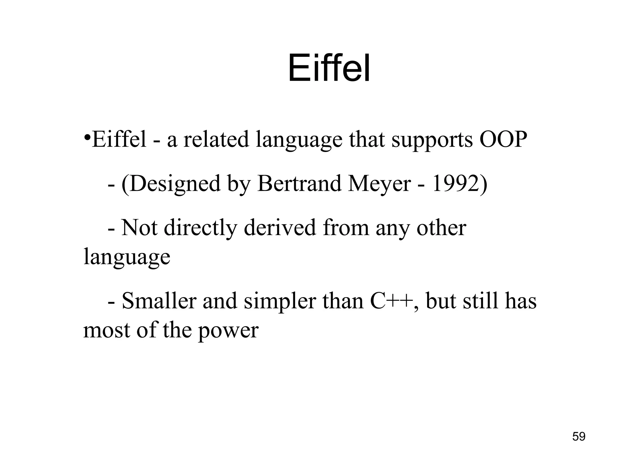
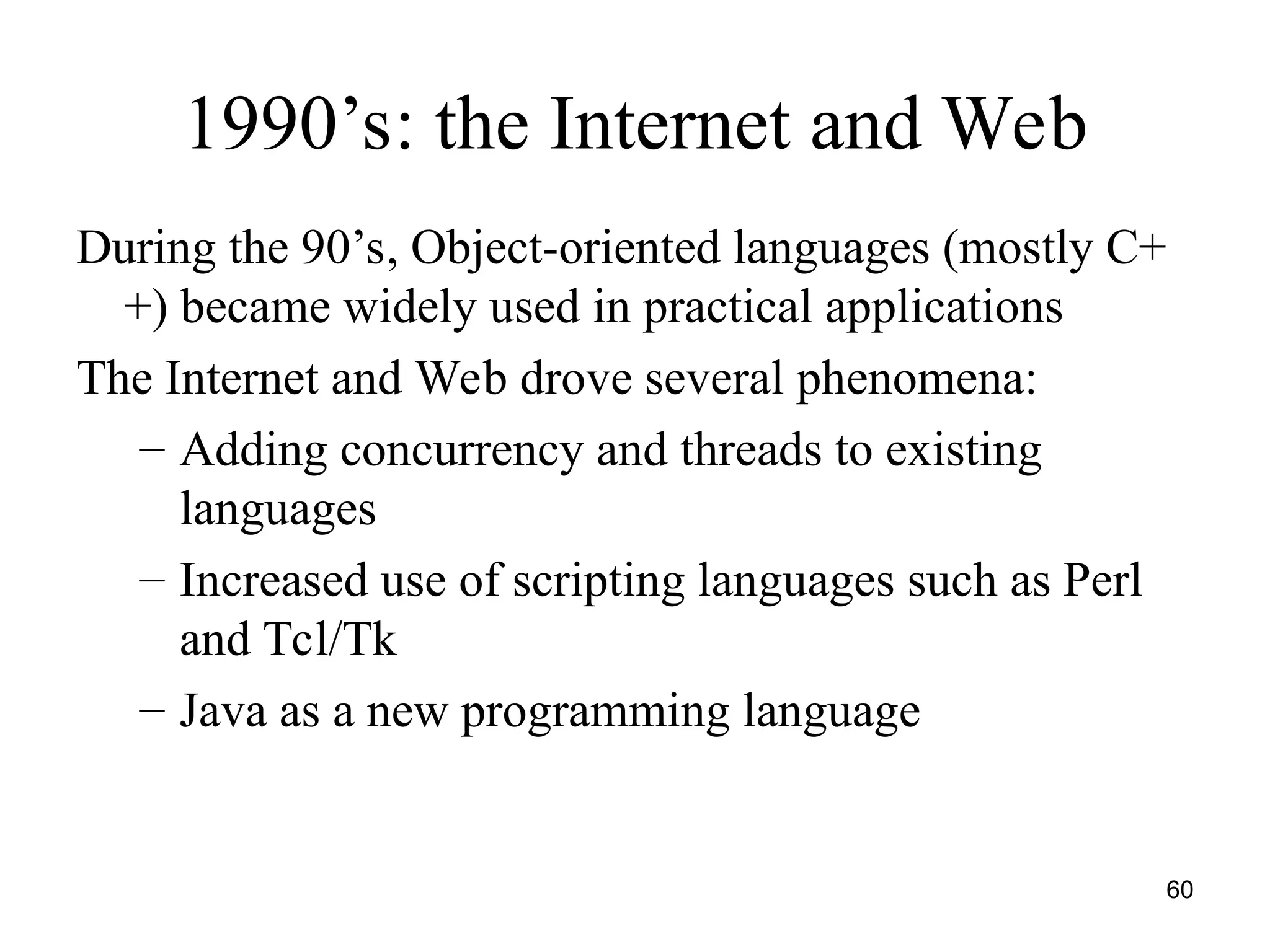
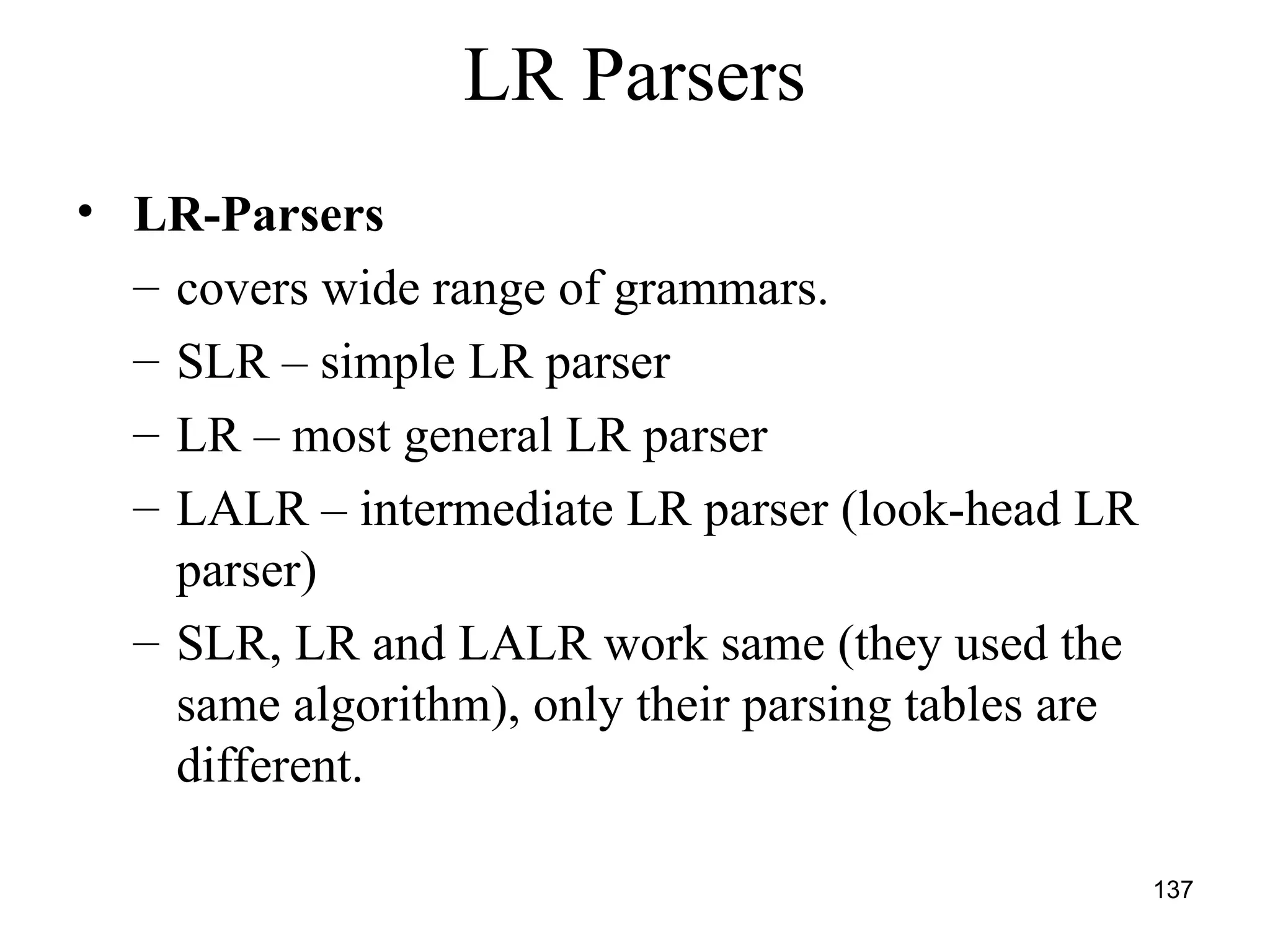
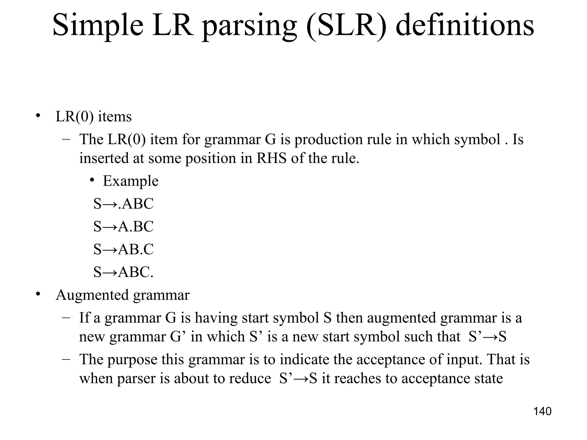
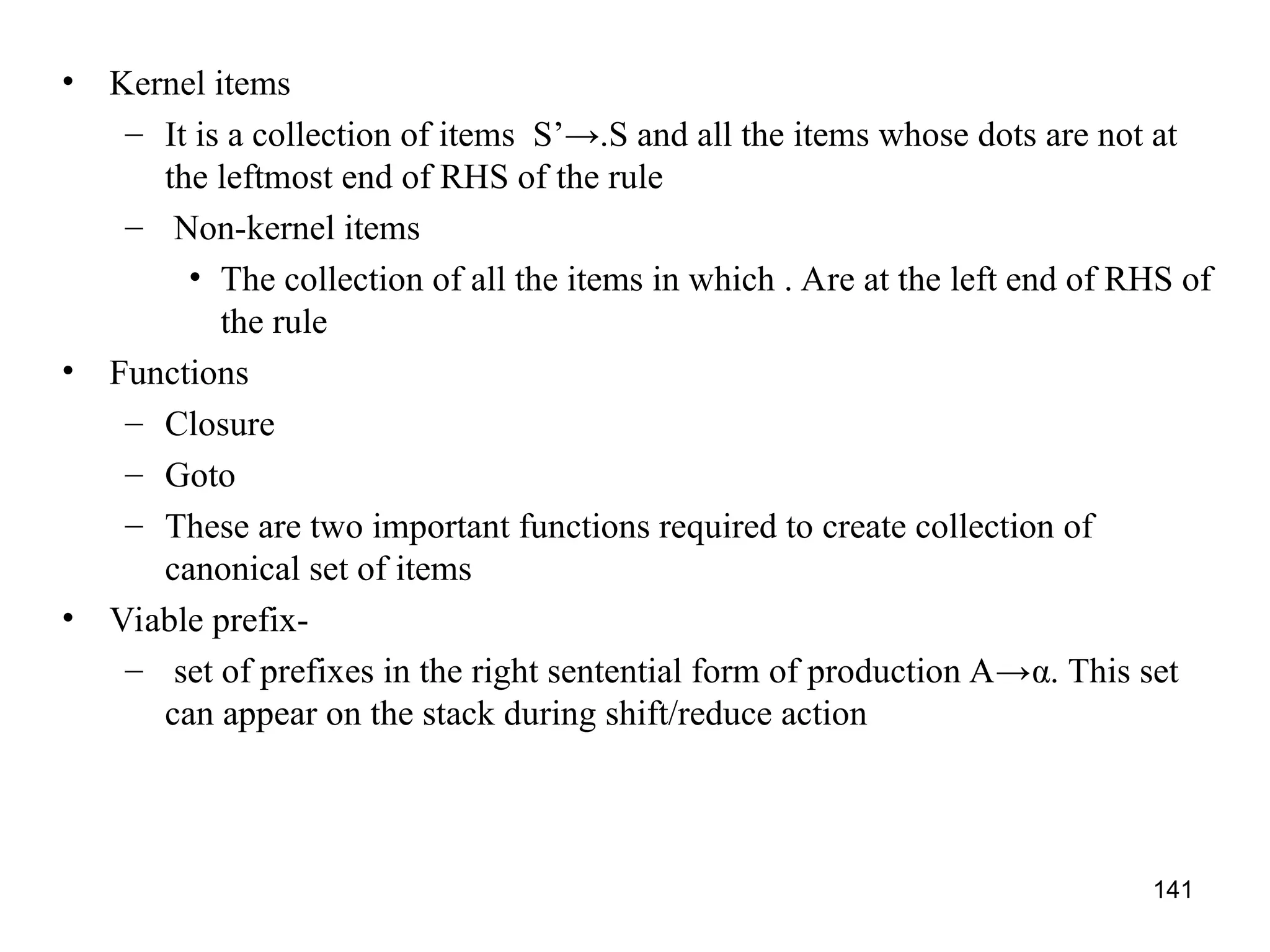
The document covers the principles of programming languages, focusing on syntax, semantics, and the evolution of programming languages, highlighting key objectives and concepts such as data types, object-orientation, and language design factors. It explores the historical development of various programming languages including Fortran, COBOL, Lisp, and Algol, detailing their features, design goals, and contributions to programming. The document emphasizes the importance of language characteristics like simplicity, reliability, and efficient implementation in effective programming.

![Extended Backus-Naur Form
(EBNF)
• Optional parts are placed in brackets ([ ])
• <proc_call> → ident [(<expr_list>)]
• Alternative parts of RHSs are placed inside parentheses and separated
via vertical bars
• <term> → <term> (+|-) const
• Repetitions (0 or more) are placed inside braces ({ })
• <ident> → letter {letter|digit}
72](https://image.slidesharecdn.com/unit1-241219071402-877eb3ad/75/PPL-unit-1-syntax-and-semantics-evolution-of-programming-language-lexical-analysis-72-2048.jpg)
![Example
• Syntax
<assign> → <var> = <expr>
<expr> → <var> + <var> | <var>
<var> → A | B | C
• actual_type: synthesized for <var> and <expr>
• expected_type: inherited for <expr>
• Syntax rule :<expr> → <var>[1] + <var>[2]
• Semantic rules :<expr>.actual_type → <var>[1].actual_type
• Predicate :<var>[1].actual_type == <var>[2].actual_type
• <expr>.expected_type == <expr>.actual_type
• Syntax rule :<var> → id
• Semantic rule :<var>.actual_type lookup (<var>.string)
76](https://image.slidesharecdn.com/unit1-241219071402-877eb3ad/75/PPL-unit-1-syntax-and-semantics-evolution-of-programming-language-lexical-analysis-76-2048.jpg)
![How are attribute values
computed?
• – If all attributes were inherited, the tree could be decorated in top-down
order.
• – If all attributes were synthesized, the tree could be decorated in bottom-
up order.
• – In many cases, both kinds of attributes are used, and it is some
combination of top-down and bottom-up that must be used.
<expr>.expected_type inherited from parent
<var>[1].actual_type lookup (A)
<var>[2].actual_type lookup (B)
<var>[1].actual_type =? <var>[2].actual_type
<expr>.actual_type <var>[1].actual_type
<expr>.actual_type =? <expr>.expected_type
77](https://image.slidesharecdn.com/unit1-241219071402-877eb3ad/75/PPL-unit-1-syntax-and-semantics-evolution-of-programming-language-lexical-analysis-77-2048.jpg)
![90
• We frequently use the following shorthands:
r+
= rr*
r? = r |
[a-z] = a | b | c | … | z
• For example:
digit [0-9]
num digit+
(. digit+
)? ( E (+|-)? digit+
)?](https://image.slidesharecdn.com/unit1-241219071402-877eb3ad/75/PPL-unit-1-syntax-and-semantics-evolution-of-programming-language-lexical-analysis-90-2048.jpg)

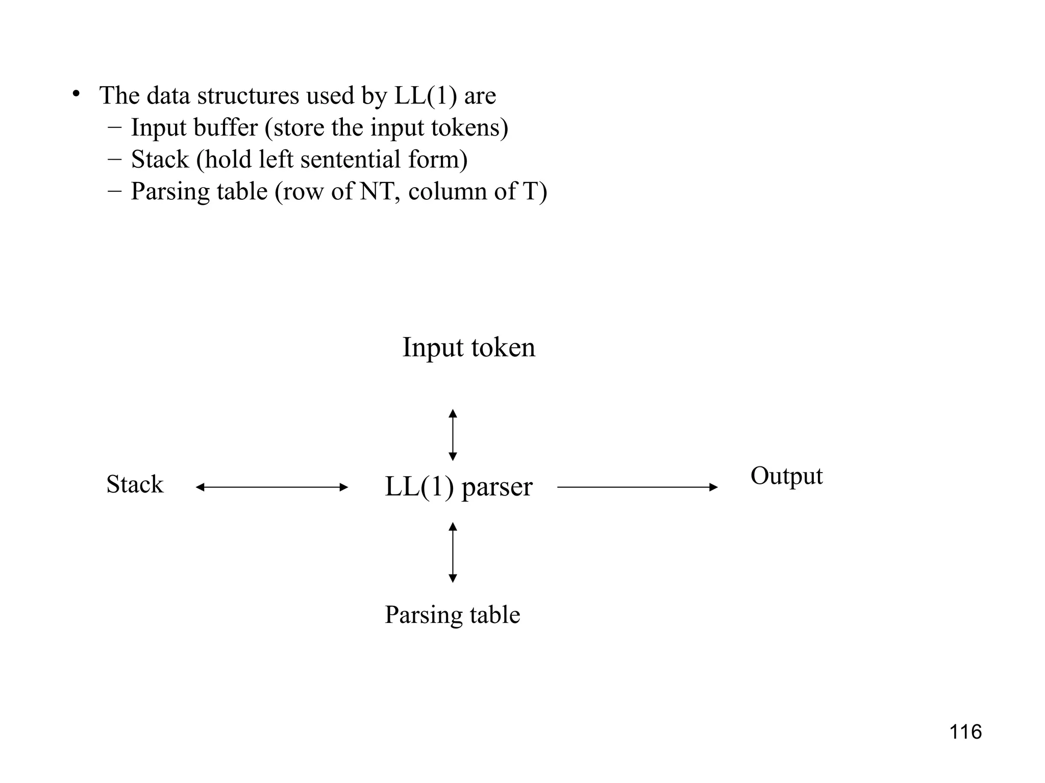
![117
LL(1) Parser
input buffer
– our string to be parsed. We will assume that its end is marked with a special symbol $.
output
– a production rule representing a step of the derivation sequence (left-most derivation) of the string
in the input buffer.
stack
– contains the grammar symbols
– at the bottom of the stack, there is a special end marker symbol $.
– initially the stack contains only the symbol $ and the starting symbol S. $S initial stack
– when the stack is emptied (ie. only $ left in the stack), the parsing is completed.
parsing table
– a two-dimensional array M[A,a]
– each row is a non-terminal symbol
– each column is a terminal symbol or the special symbol $
– each entry holds a production rule.](https://image.slidesharecdn.com/unit1-241219071402-877eb3ad/75/PPL-unit-1-syntax-and-semantics-evolution-of-programming-language-lexical-analysis-117-2048.jpg)
![118
LL(1) Parser – Parser Actions
• The symbol at the top of the stack (say X) and the current symbol in the input
string (say a) determine the parser action.
• There are four possible parser actions.
1. If X and a are $ → parser halts (successful completion)
2. If X and a are the same terminal symbol (different from $)
→ parser pops X from the stack, and moves the next symbol in the input buffer.
3. If X is a non-terminal
→ parser looks at the parsing table entry M[X,a]. If M[X,a] holds a production
rule XY1Y2...Yk, it pops X from the stack and pushes Yk,Yk-1,...,Y1 into the
stack. The parser also outputs the production rule XY1Y2...Yk to represent a
step of the derivation.
4. none of the above → error
– all empty entries in the parsing table are errors.
– If X is a terminal symbol different from a, this is also an error case.](https://image.slidesharecdn.com/unit1-241219071402-877eb3ad/75/PPL-unit-1-syntax-and-semantics-evolution-of-programming-language-lexical-analysis-118-2048.jpg)
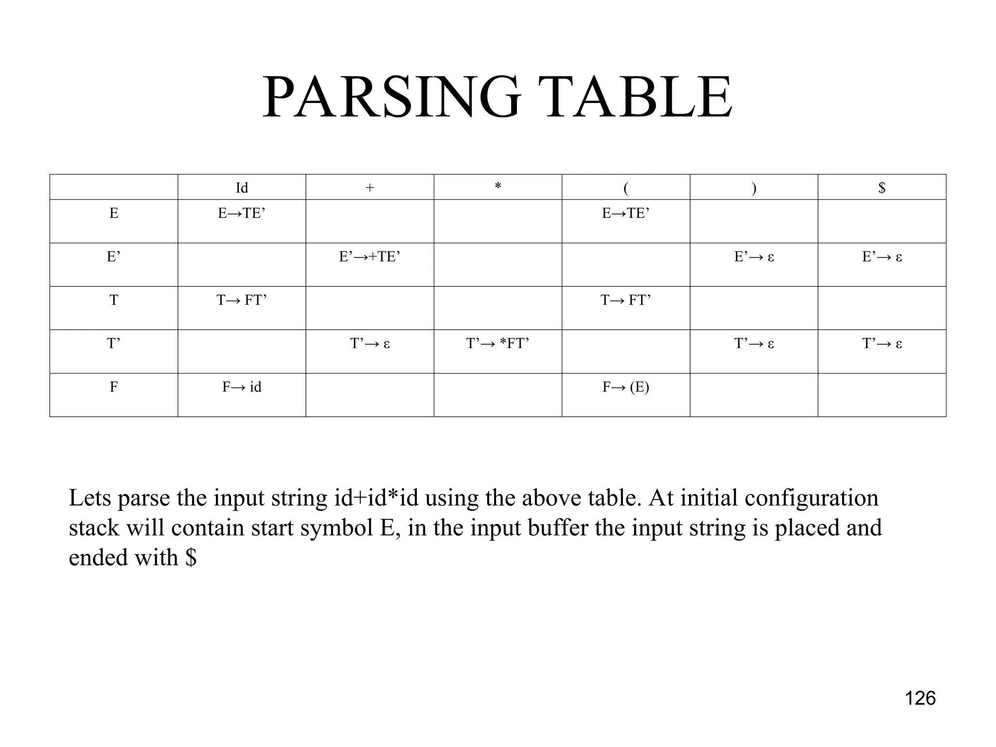
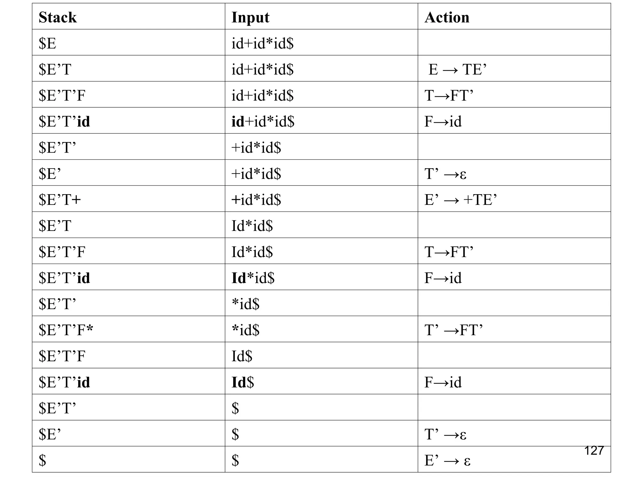
![125
Predictive parsing table construction
• For the rule A →α of grammar G
1. For each a in FIRST(α) create M[A,a] = A →α
where a is a terminal symbol
2. For ε in FIRST(α) create entry in M[A,b] = A
→α where b is the symbols from FOLLOW(A)
3. If ε is in FIRST(α) and $ is in FOLLOW(A) then
create entry in the table M[A,$] = A →α
4. All the remaining entries in the table M are
marked as ERROR](https://image.slidesharecdn.com/unit1-241219071402-877eb3ad/75/PPL-unit-1-syntax-and-semantics-evolution-of-programming-language-lexical-analysis-125-2048.jpg)
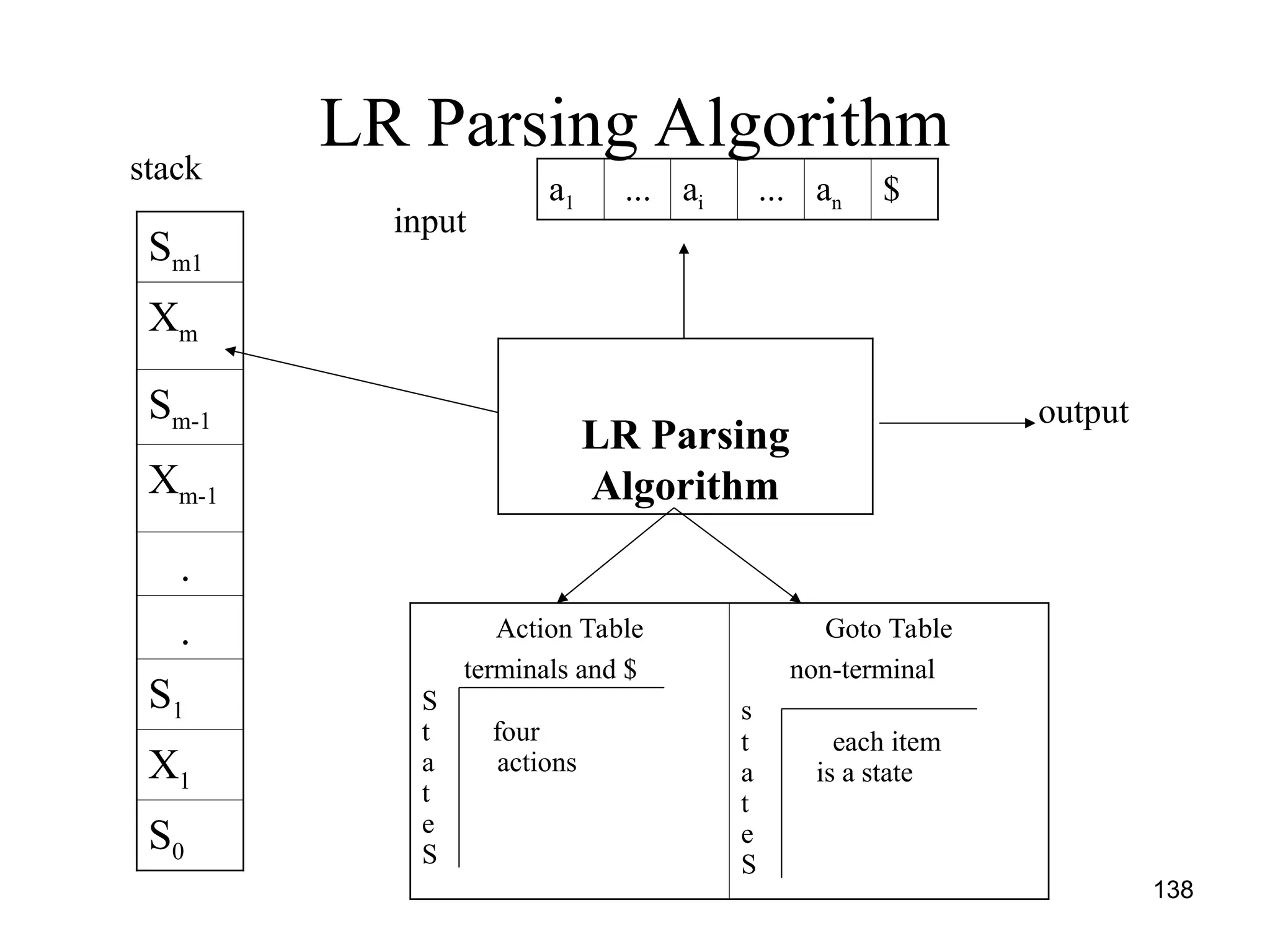
![139
Parsing method
• Initialize the stack with start symbol and invokes
scanner to get next token
• It determines Sj the state currently on the top of the
stack and ai the current input symbol
• It consults the parsing table for the action [Sj, ai] which
can have one of the four values
– Si means shift state I
– rj means reduce by rule j
– Accept means successful parsing is done
– Error indicates syntactical error](https://image.slidesharecdn.com/unit1-241219071402-877eb3ad/75/PPL-unit-1-syntax-and-semantics-evolution-of-programming-language-lexical-analysis-139-2048.jpg)
![149
STACK INPUT
BUFFER
ACTION
TABLE
GOTO
TABLE
PARSING
ACTION
$0 Id*id*id$ [0,id]=s5 Shift
$0id5 *id+id$ [5,*]=r6 [0,f]=3 Reduce
F→id
$0F3 *id*id$ [3,*]=r4 [0,T]=2 Reduce T→F
$0T2 *id+id$ [2,*]=s7 Shift
$0T2*7 Id+id$ [7,id]=s5 Shift
$0T2*7id5 +id$ [5,+]=r6 [7,F]=10 reduce
$0T2*7F10 +id$ [10,+]=r3 [0,T]=2 Reduce
$0T2 +id$ [2,+]=r2 [0,E]=1 Reduce
$0E1 +id$ [1,=]=s6 Shift
$0E1+6 +id$ [6,id]=s5 Shift
$0E1+6ID5 $ [5,$]=r6 [6,F]=3 Reduce
$0E1+6F3 $ [3,$]=r4 [6,T]=9 Reduce
$0E1+6T9 $ [9,$]=r1 [0,E]=1 Reduce
$0E1 $ Accept accept](https://image.slidesharecdn.com/unit1-241219071402-877eb3ad/75/PPL-unit-1-syntax-and-semantics-evolution-of-programming-language-lexical-analysis-149-2048.jpg)
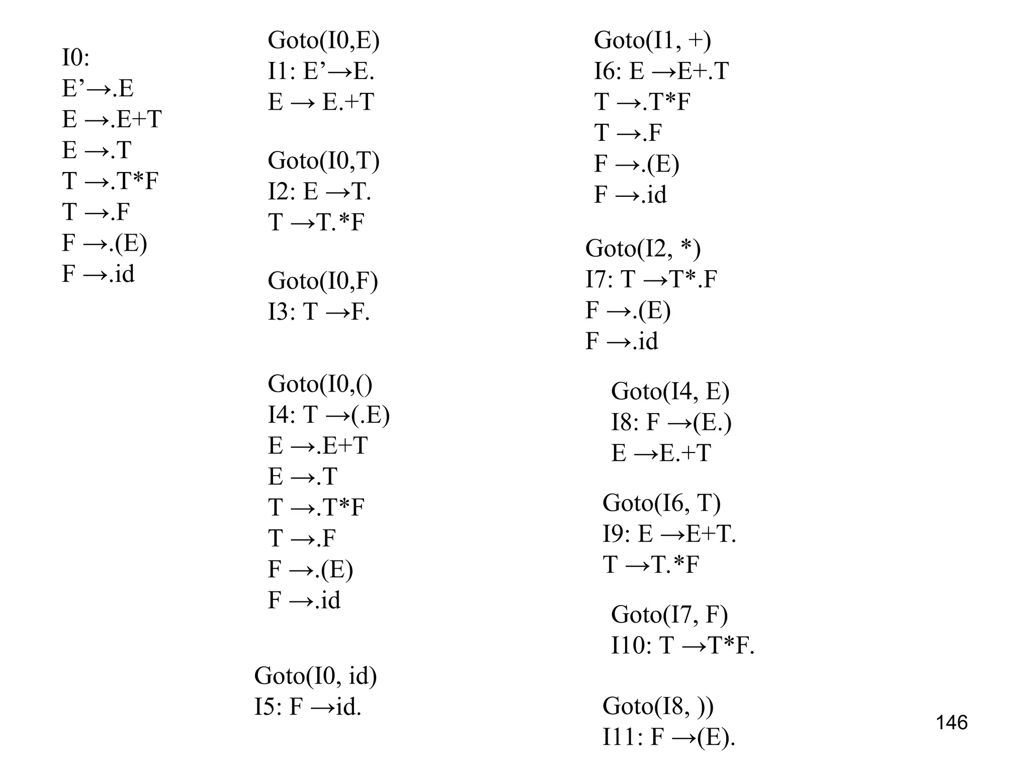
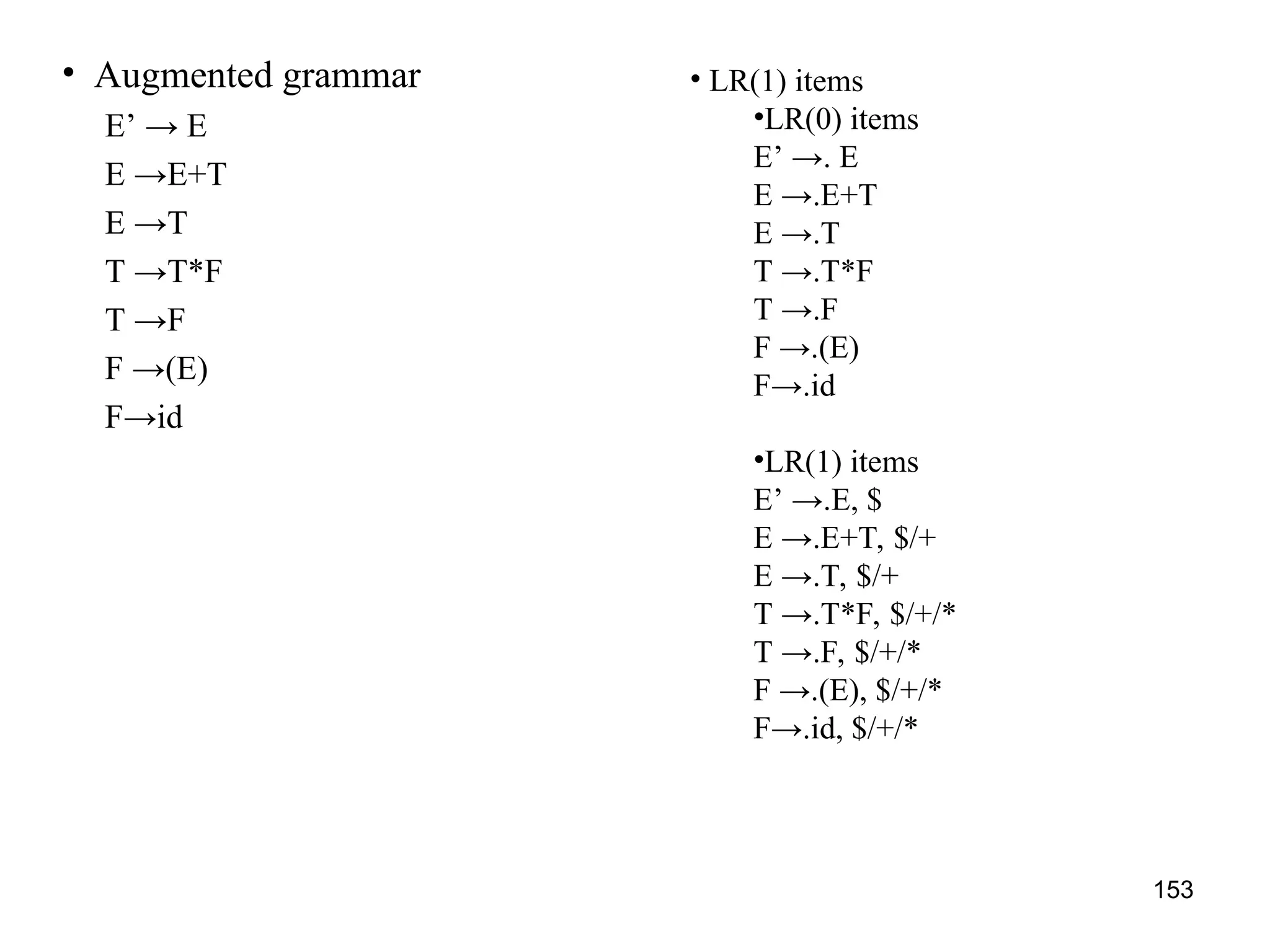
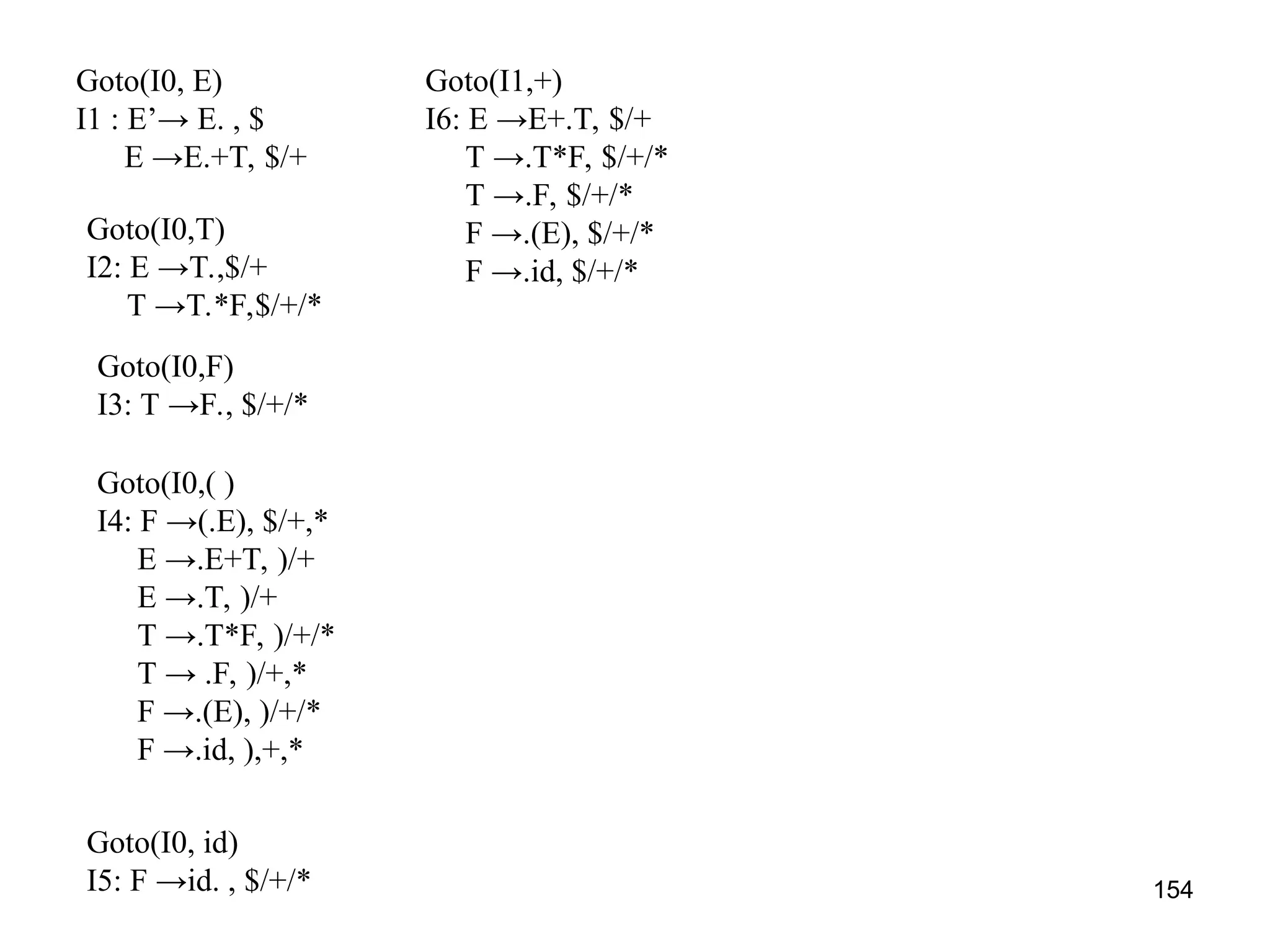
![150
CLR PARSING or LR(1)
PARSING
• Construction of canonical set of items along with lookahead
• For the grammar G initially add S’→.S in the set of item C
• For each set of items Ii in C and for each grammar symbol X (T ot
NT) add closure(Ii,X). This process is repeated by applying
goto(Ii,X) for each X in Ii such that goto(Ii,X) is not empty and not
in C. The set of items has to constructed until no more set of items
can be added to C
• The closure function can be computed as : for each item
[A→α.Xβ, a] is in I and rule [A→αX.β, a] is not in goto items
then add [A→αX.β, a] to goto items
• This process is repeated until no more set of items can be added to
the collection C](https://image.slidesharecdn.com/unit1-241219071402-877eb3ad/75/PPL-unit-1-syntax-and-semantics-evolution-of-programming-language-lexical-analysis-150-2048.jpg)
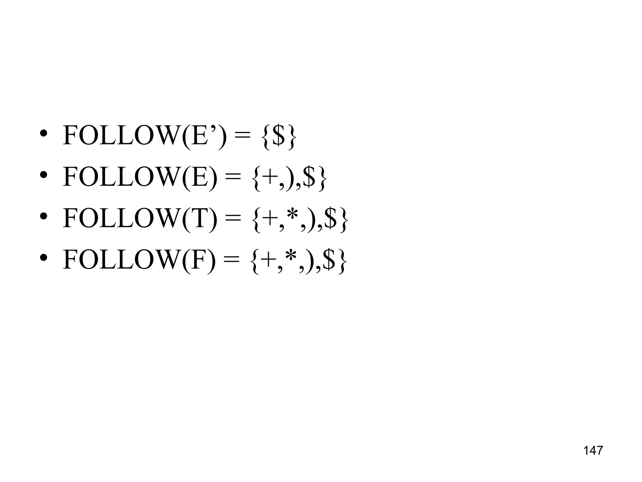
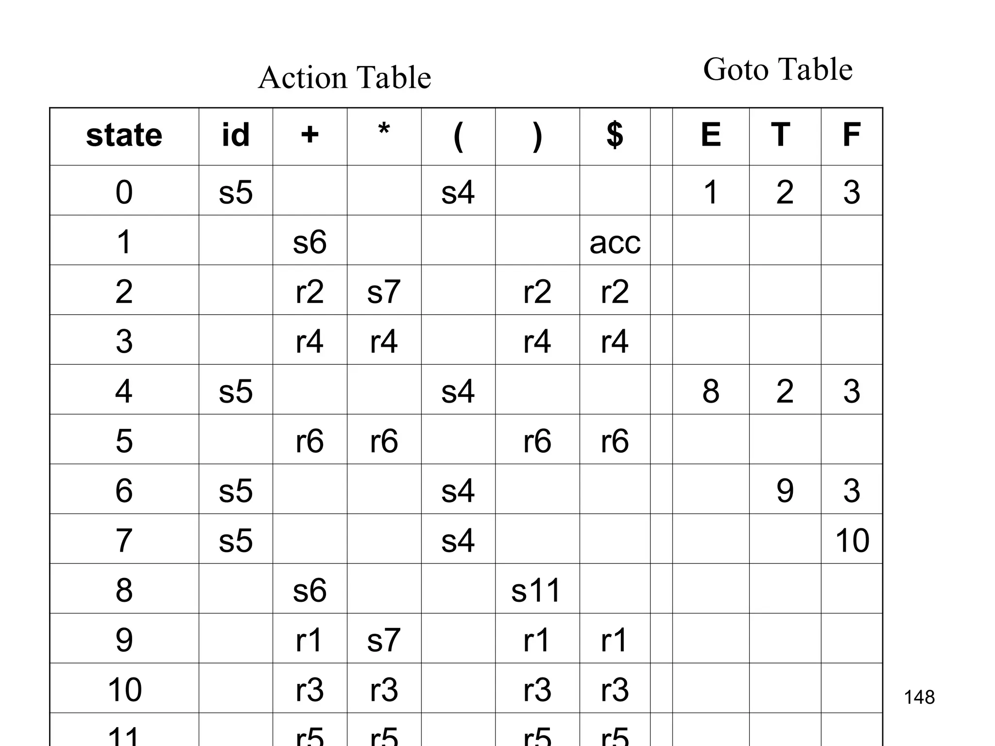
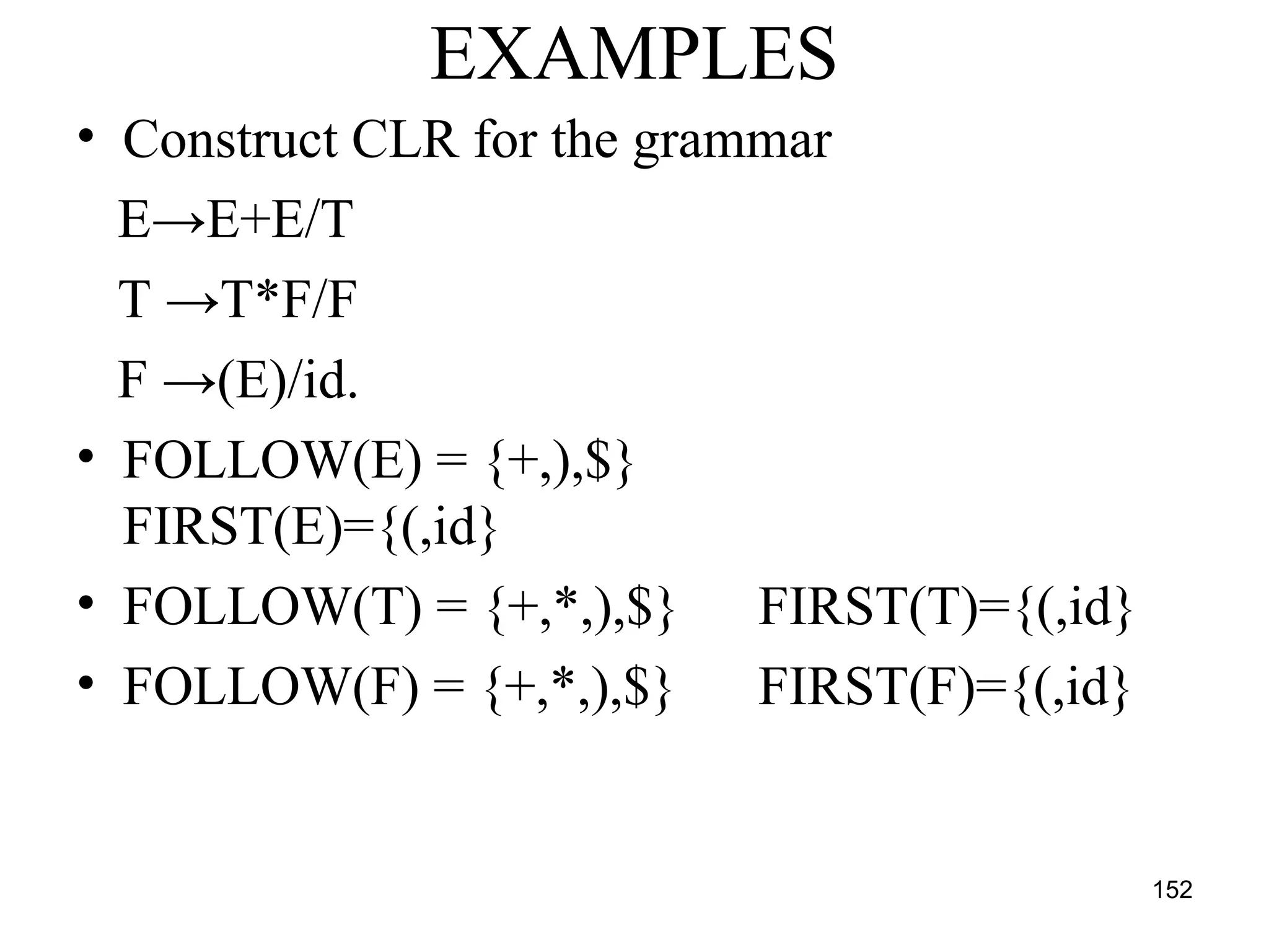
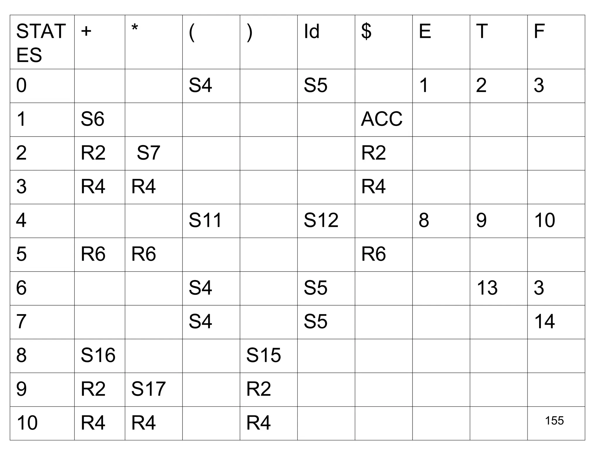
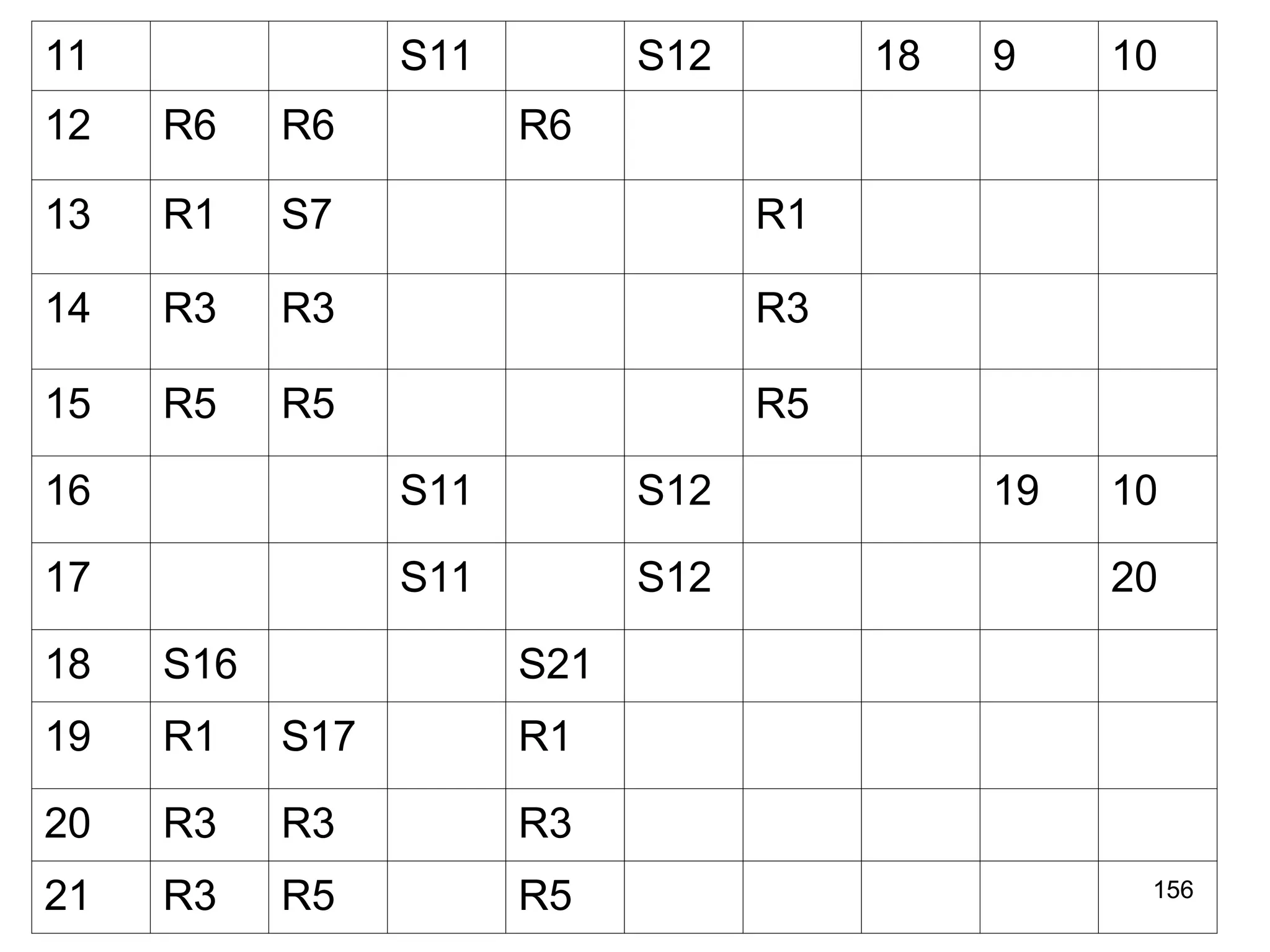
![151
CONSTRUCTION OF CLR PARSING TABLE
• Construct set of items C={I0,I1,I2,...In} where C is a collection of
set of LR(1) items for the input grammar G’.
• The parsing actions are based on each items Ii.
– If [A→αBβ, b] is in Ii and goto(Ii, a)=Ii then create a entry in the action
table action[Ii,a]=shift j.
– If there is a production A→α., a] in Ii then in action table
action[Ii,a]=reduce by A→α. Here A should not be S’.
– If there is a production S’ →S.,$ in Ii then action[i,$]=accept.
• The goto part of LR table can be filled as: the goto transition for
state i is considered for NT only. If goto(Ii,A)=Ij, then
goto(Ii,A)=j
• All other entries are defined as ERROR](https://image.slidesharecdn.com/unit1-241219071402-877eb3ad/75/PPL-unit-1-syntax-and-semantics-evolution-of-programming-language-lexical-analysis-151-2048.jpg)
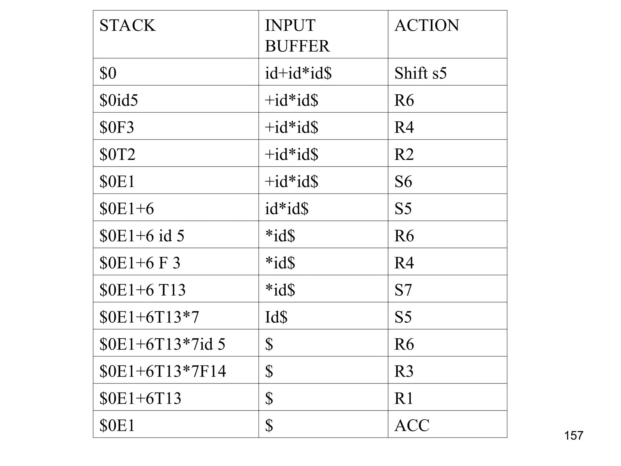
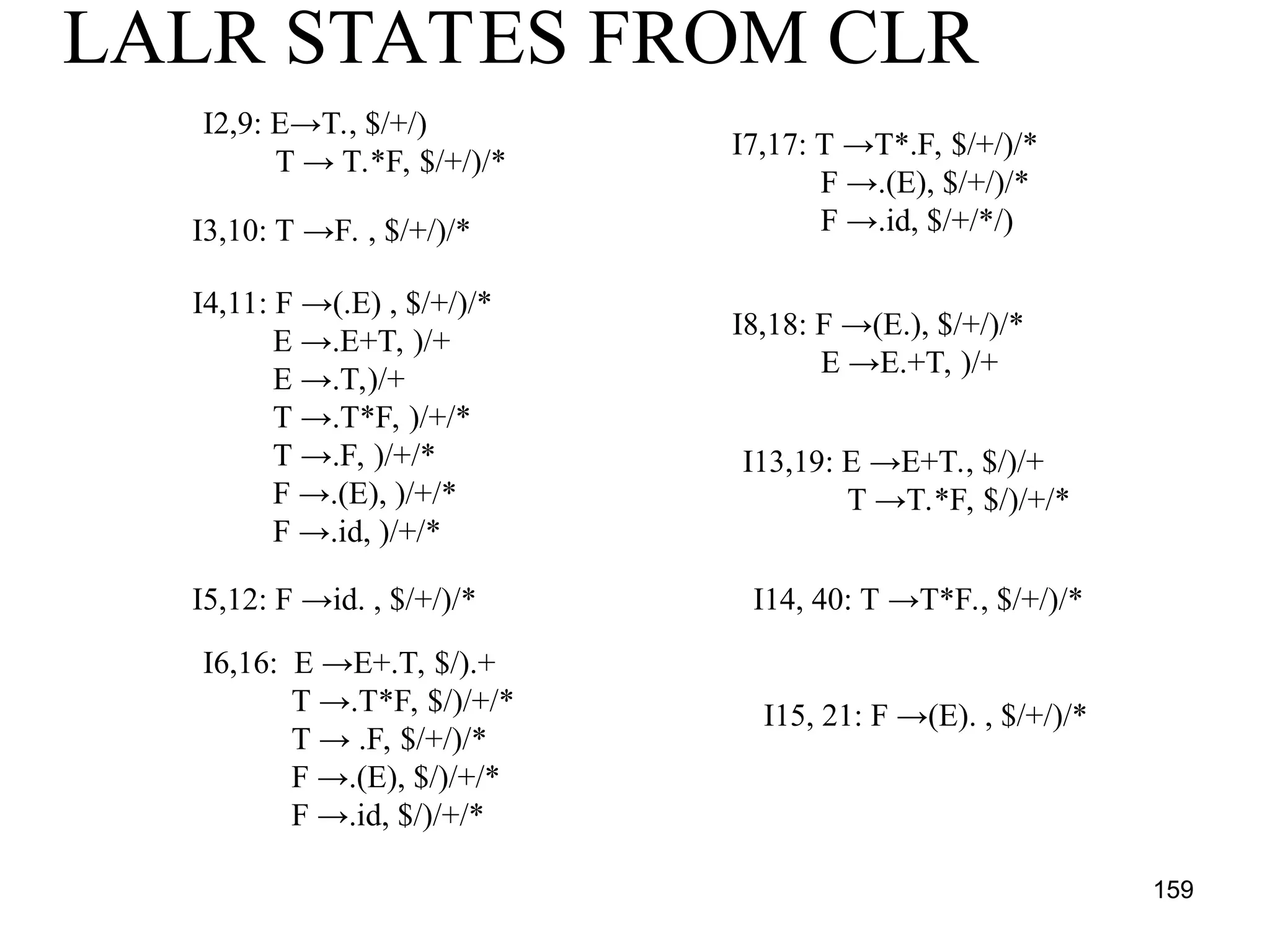
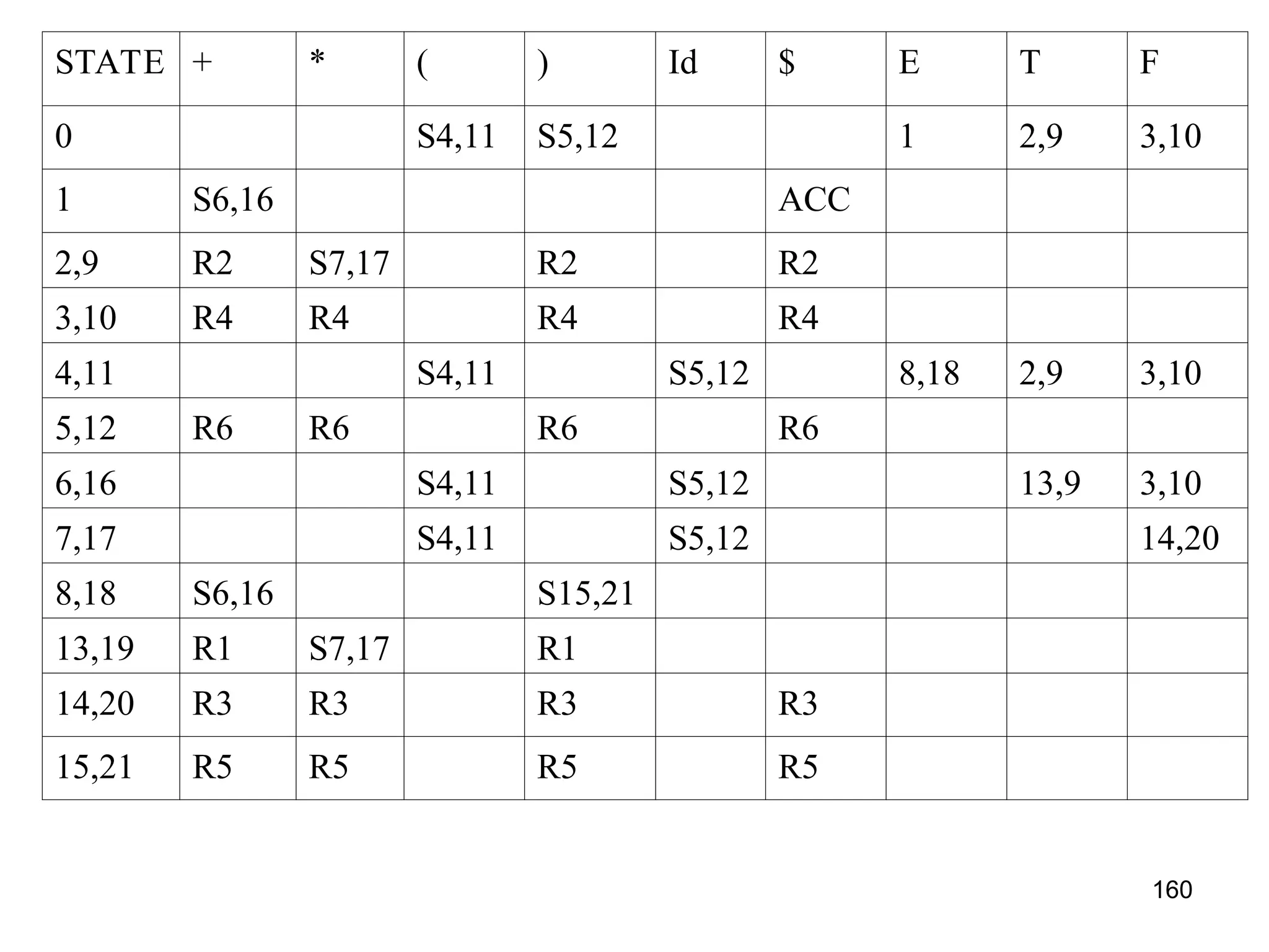
![158
LALR PARSING
• Construction of LALR parsing table
• Construct LR(1) items
• Merge two states Ii and Ij if the first component are matching and create
a new state replacing one of the older states such as Iij = Ii U Ij
• The parsing actions are based on each item Ii.
– If [A→α.aβ, b] is in Ii and goto(Ii,a)=Ij then create an entry in the action table
action[Ii,a]= shift j
– If there is a production [A→α., a] in Ii then in the action table action[Ii,a]=reduce
by A→α. Here A should not be S’.
– If there is a production S’ →S,$ in Ii then action[i,$]=accept
• The goto part : the goto transitions for state i is considered for NTonly.
If goto(Ii,A)=Ij, then goto[Ii,A]=j
• If the parsing action conflicts, then the grammar is not LALR(1). All
other entries are ERROR](https://image.slidesharecdn.com/unit1-241219071402-877eb3ad/75/PPL-unit-1-syntax-and-semantics-evolution-of-programming-language-lexical-analysis-158-2048.jpg)


![Extended Backus-Naur Form
(EBNF)
• Optional parts are placed in brackets ([ ])
• <proc_call> → ident [(<expr_list>)]
• Alternative parts of RHSs are placed inside parentheses and separated
via vertical bars
• <term> → <term> (+|-) const
• Repetitions (0 or more) are placed inside braces ({ })
• <ident> → letter {letter|digit}
72](https://crownmelresort.com/image.slidesharecdn.com/unit1-241219071402-877eb3ad/75/PPL-unit-1-syntax-and-semantics-evolution-of-programming-language-lexical-analysis-72-2048.jpg)


![Example
• Syntax
<assign> → <var> = <expr>
<expr> → <var> + <var> | <var>
<var> → A | B | C
• actual_type: synthesized for <var> and <expr>
• expected_type: inherited for <expr>
• Syntax rule :<expr> → <var>[1] + <var>[2]
• Semantic rules :<expr>.actual_type → <var>[1].actual_type
• Predicate :<var>[1].actual_type == <var>[2].actual_type
• <expr>.expected_type == <expr>.actual_type
• Syntax rule :<var> → id
• Semantic rule :<var>.actual_type lookup (<var>.string)
76](https://crownmelresort.com/image.slidesharecdn.com/unit1-241219071402-877eb3ad/75/PPL-unit-1-syntax-and-semantics-evolution-of-programming-language-lexical-analysis-76-2048.jpg)
![How are attribute values
computed?
• – If all attributes were inherited, the tree could be decorated in top-down
order.
• – If all attributes were synthesized, the tree could be decorated in bottom-
up order.
• – In many cases, both kinds of attributes are used, and it is some
combination of top-down and bottom-up that must be used.
<expr>.expected_type inherited from parent
<var>[1].actual_type lookup (A)
<var>[2].actual_type lookup (B)
<var>[1].actual_type =? <var>[2].actual_type
<expr>.actual_type <var>[1].actual_type
<expr>.actual_type =? <expr>.expected_type
77](https://crownmelresort.com/image.slidesharecdn.com/unit1-241219071402-877eb3ad/75/PPL-unit-1-syntax-and-semantics-evolution-of-programming-language-lexical-analysis-77-2048.jpg)


![90
• We frequently use the following shorthands:
r+
= rr*
r? = r |
[a-z] = a | b | c | … | z
• For example:
digit [0-9]
num digit+
(. digit+
)? ( E (+|-)? digit+
)?](https://crownmelresort.com/image.slidesharecdn.com/unit1-241219071402-877eb3ad/75/PPL-unit-1-syntax-and-semantics-evolution-of-programming-language-lexical-analysis-90-2048.jpg)


![117
LL(1) Parser
input buffer
– our string to be parsed. We will assume that its end is marked with a special symbol $.
output
– a production rule representing a step of the derivation sequence (left-most derivation) of the string
in the input buffer.
stack
– contains the grammar symbols
– at the bottom of the stack, there is a special end marker symbol $.
– initially the stack contains only the symbol $ and the starting symbol S. $S initial stack
– when the stack is emptied (ie. only $ left in the stack), the parsing is completed.
parsing table
– a two-dimensional array M[A,a]
– each row is a non-terminal symbol
– each column is a terminal symbol or the special symbol $
– each entry holds a production rule.](https://crownmelresort.com/image.slidesharecdn.com/unit1-241219071402-877eb3ad/75/PPL-unit-1-syntax-and-semantics-evolution-of-programming-language-lexical-analysis-117-2048.jpg)
![118
LL(1) Parser – Parser Actions
• The symbol at the top of the stack (say X) and the current symbol in the input
string (say a) determine the parser action.
• There are four possible parser actions.
1. If X and a are $ → parser halts (successful completion)
2. If X and a are the same terminal symbol (different from $)
→ parser pops X from the stack, and moves the next symbol in the input buffer.
3. If X is a non-terminal
→ parser looks at the parsing table entry M[X,a]. If M[X,a] holds a production
rule XY1Y2...Yk, it pops X from the stack and pushes Yk,Yk-1,...,Y1 into the
stack. The parser also outputs the production rule XY1Y2...Yk to represent a
step of the derivation.
4. none of the above → error
– all empty entries in the parsing table are errors.
– If X is a terminal symbol different from a, this is also an error case.](https://crownmelresort.com/image.slidesharecdn.com/unit1-241219071402-877eb3ad/75/PPL-unit-1-syntax-and-semantics-evolution-of-programming-language-lexical-analysis-118-2048.jpg)


![125
Predictive parsing table construction
• For the rule A →α of grammar G
1. For each a in FIRST(α) create M[A,a] = A →α
where a is a terminal symbol
2. For ε in FIRST(α) create entry in M[A,b] = A
→α where b is the symbols from FOLLOW(A)
3. If ε is in FIRST(α) and $ is in FOLLOW(A) then
create entry in the table M[A,$] = A →α
4. All the remaining entries in the table M are
marked as ERROR](https://crownmelresort.com/image.slidesharecdn.com/unit1-241219071402-877eb3ad/75/PPL-unit-1-syntax-and-semantics-evolution-of-programming-language-lexical-analysis-125-2048.jpg)


![139
Parsing method
• Initialize the stack with start symbol and invokes
scanner to get next token
• It determines Sj the state currently on the top of the
stack and ai the current input symbol
• It consults the parsing table for the action [Sj, ai] which
can have one of the four values
– Si means shift state I
– rj means reduce by rule j
– Accept means successful parsing is done
– Error indicates syntactical error](https://crownmelresort.com/image.slidesharecdn.com/unit1-241219071402-877eb3ad/75/PPL-unit-1-syntax-and-semantics-evolution-of-programming-language-lexical-analysis-139-2048.jpg)


![149
STACK INPUT
BUFFER
ACTION
TABLE
GOTO
TABLE
PARSING
ACTION
$0 Id*id*id$ [0,id]=s5 Shift
$0id5 *id+id$ [5,*]=r6 [0,f]=3 Reduce
F→id
$0F3 *id*id$ [3,*]=r4 [0,T]=2 Reduce T→F
$0T2 *id+id$ [2,*]=s7 Shift
$0T2*7 Id+id$ [7,id]=s5 Shift
$0T2*7id5 +id$ [5,+]=r6 [7,F]=10 reduce
$0T2*7F10 +id$ [10,+]=r3 [0,T]=2 Reduce
$0T2 +id$ [2,+]=r2 [0,E]=1 Reduce
$0E1 +id$ [1,=]=s6 Shift
$0E1+6 +id$ [6,id]=s5 Shift
$0E1+6ID5 $ [5,$]=r6 [6,F]=3 Reduce
$0E1+6F3 $ [3,$]=r4 [6,T]=9 Reduce
$0E1+6T9 $ [9,$]=r1 [0,E]=1 Reduce
$0E1 $ Accept accept](https://crownmelresort.com/image.slidesharecdn.com/unit1-241219071402-877eb3ad/75/PPL-unit-1-syntax-and-semantics-evolution-of-programming-language-lexical-analysis-149-2048.jpg)
![150
CLR PARSING or LR(1)
PARSING
• Construction of canonical set of items along with lookahead
• For the grammar G initially add S’→.S in the set of item C
• For each set of items Ii in C and for each grammar symbol X (T ot
NT) add closure(Ii,X). This process is repeated by applying
goto(Ii,X) for each X in Ii such that goto(Ii,X) is not empty and not
in C. The set of items has to constructed until no more set of items
can be added to C
• The closure function can be computed as : for each item
[A→α.Xβ, a] is in I and rule [A→αX.β, a] is not in goto items
then add [A→αX.β, a] to goto items
• This process is repeated until no more set of items can be added to
the collection C](https://crownmelresort.com/image.slidesharecdn.com/unit1-241219071402-877eb3ad/75/PPL-unit-1-syntax-and-semantics-evolution-of-programming-language-lexical-analysis-150-2048.jpg)
![151
CONSTRUCTION OF CLR PARSING TABLE
• Construct set of items C={I0,I1,I2,...In} where C is a collection of
set of LR(1) items for the input grammar G’.
• The parsing actions are based on each items Ii.
– If [A→αBβ, b] is in Ii and goto(Ii, a)=Ii then create a entry in the action
table action[Ii,a]=shift j.
– If there is a production A→α., a] in Ii then in action table
action[Ii,a]=reduce by A→α. Here A should not be S’.
– If there is a production S’ →S.,$ in Ii then action[i,$]=accept.
• The goto part of LR table can be filled as: the goto transition for
state i is considered for NT only. If goto(Ii,A)=Ij, then
goto(Ii,A)=j
• All other entries are defined as ERROR](https://crownmelresort.com/image.slidesharecdn.com/unit1-241219071402-877eb3ad/75/PPL-unit-1-syntax-and-semantics-evolution-of-programming-language-lexical-analysis-151-2048.jpg)


![158
LALR PARSING
• Construction of LALR parsing table
• Construct LR(1) items
• Merge two states Ii and Ij if the first component are matching and create
a new state replacing one of the older states such as Iij = Ii U Ij
• The parsing actions are based on each item Ii.
– If [A→α.aβ, b] is in Ii and goto(Ii,a)=Ij then create an entry in the action table
action[Ii,a]= shift j
– If there is a production [A→α., a] in Ii then in the action table action[Ii,a]=reduce
by A→α. Here A should not be S’.
– If there is a production S’ →S,$ in Ii then action[i,$]=accept
• The goto part : the goto transitions for state i is considered for NTonly.
If goto(Ii,A)=Ij, then goto[Ii,A]=j
• If the parsing action conflicts, then the grammar is not LALR(1). All
other entries are ERROR](https://crownmelresort.com/image.slidesharecdn.com/unit1-241219071402-877eb3ad/75/PPL-unit-1-syntax-and-semantics-evolution-of-programming-language-lexical-analysis-158-2048.jpg)