Download to read offline
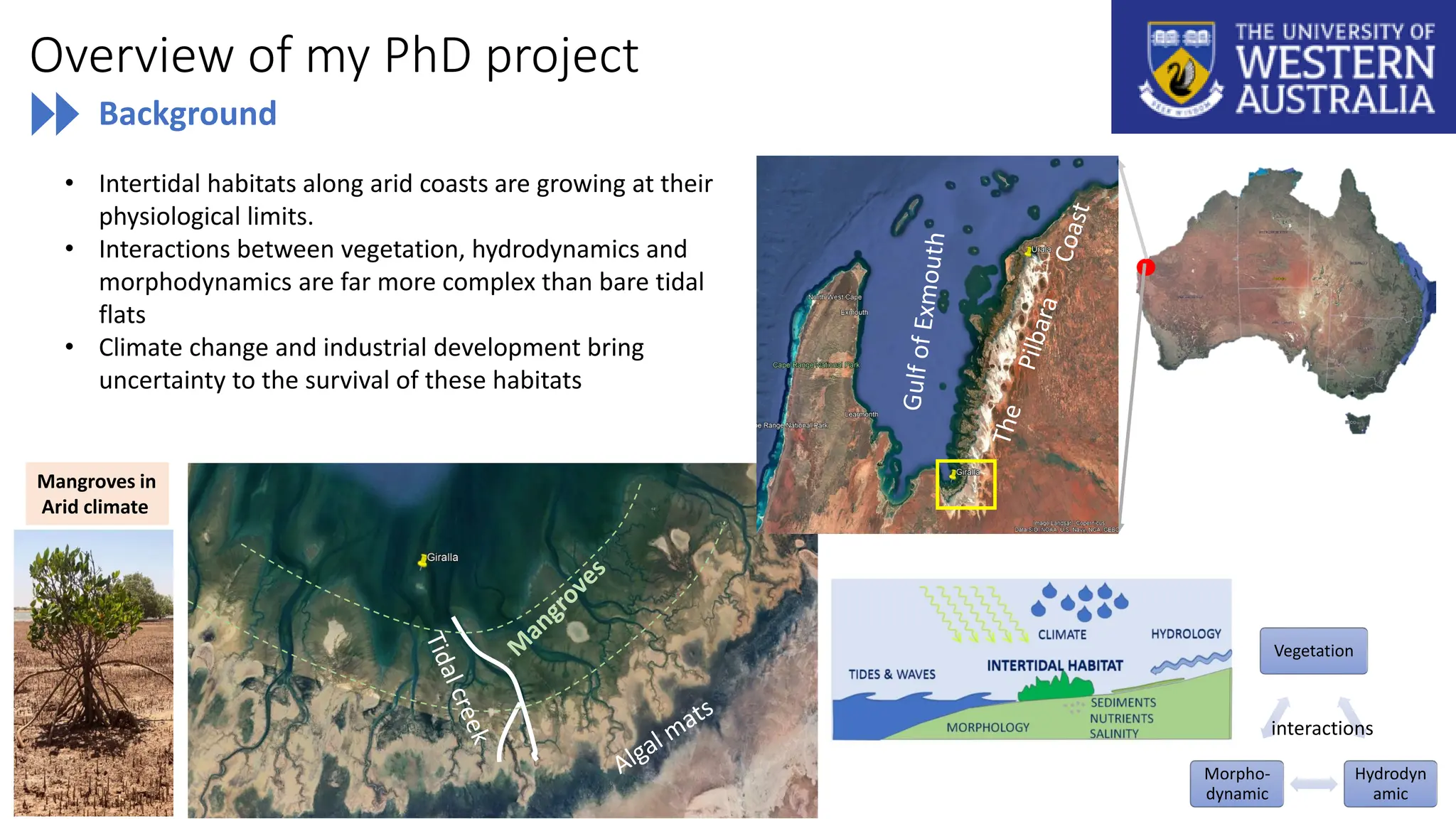
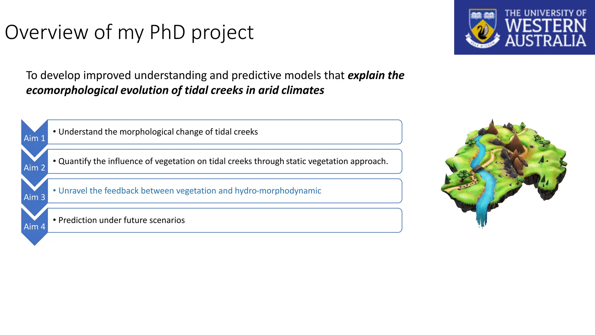
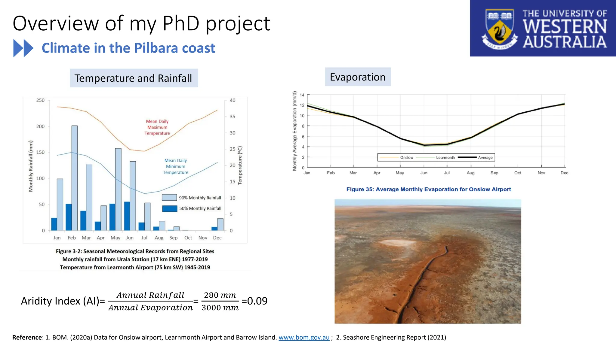
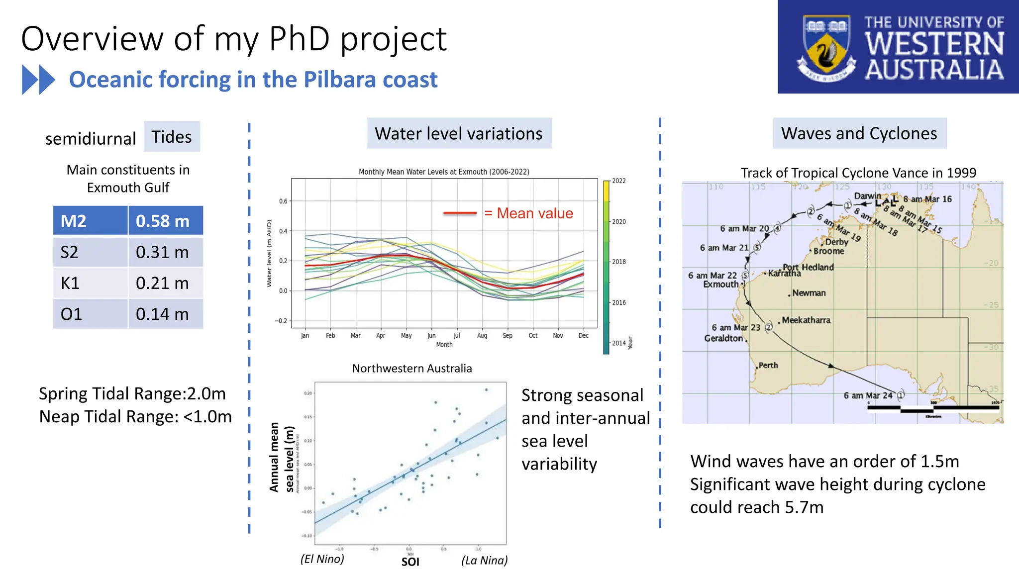
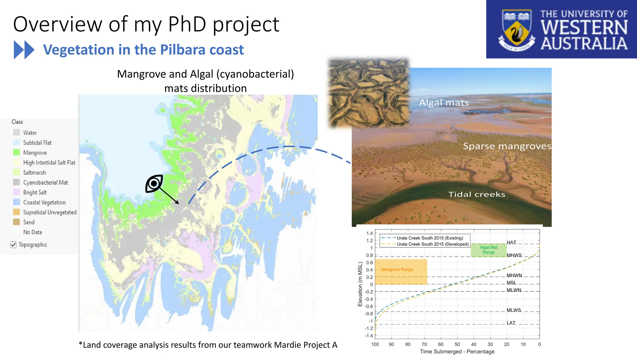
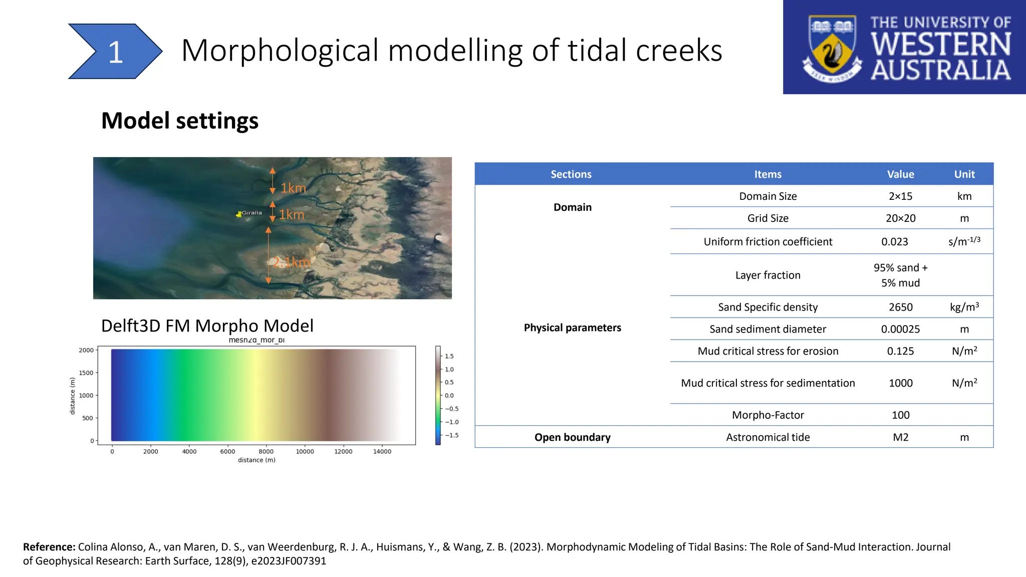


The document details a PhD project focused on morphological modeling of tidal creeks in arid coastal environments, examining the complex interactions between hydrodynamics, vegetation, and morphodynamics, particularly concerning mangroves. It outlines specific research aims including understanding morphological changes and predicting future scenarios influenced by climate change. The project leverages various modeling approaches and empirical data to assess the impacts on tidal creek evolution and the resilience of intertidal habitats.