matlab tutorial with separate function description and handson learning

Tutorial on Matlab Basics
EECS 639
August 31, 2016

Matlab Basics
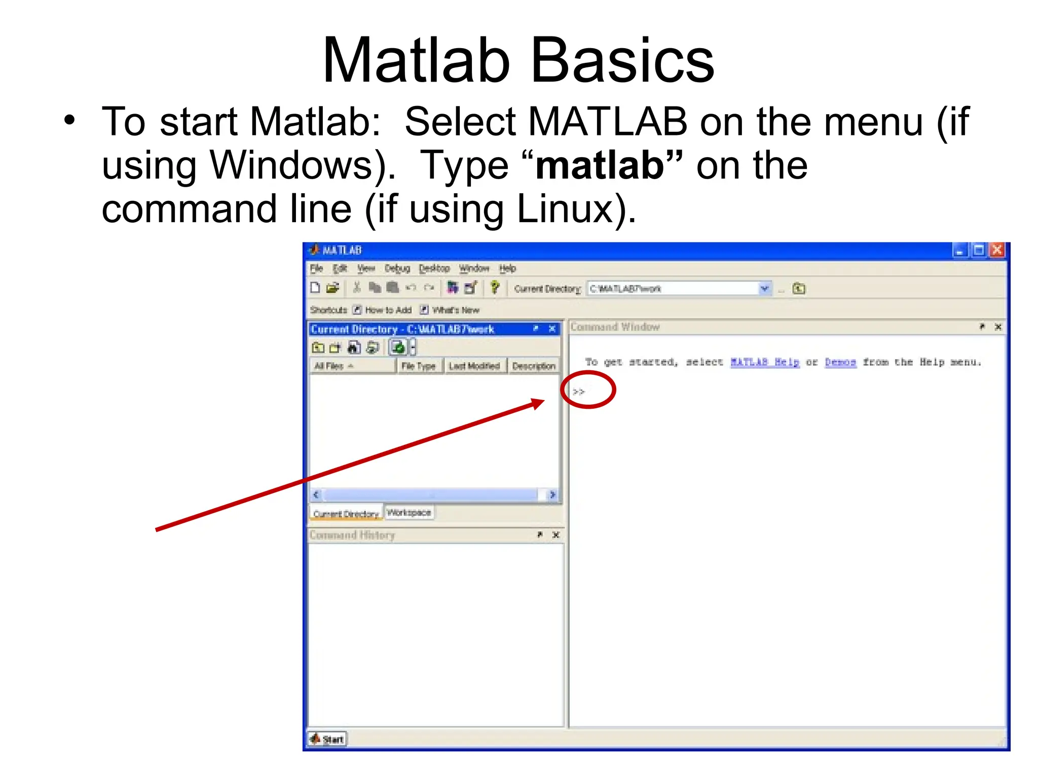
• To start Matlab: Select MATLAB on the menu (if
using Windows). Type “matlab” on the
command line (if using Linux).

Getting Help and
Looking Up Functions
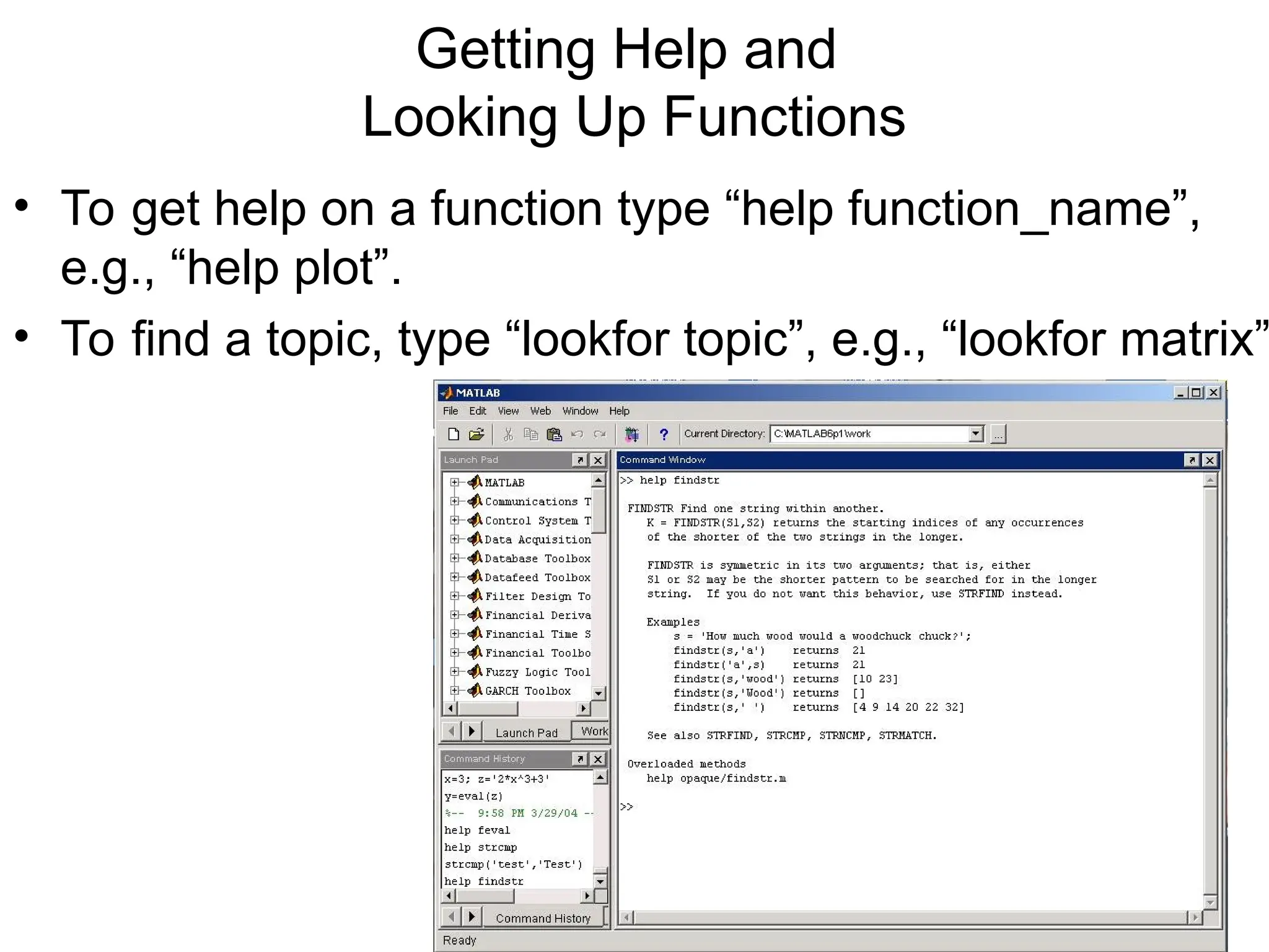
• To get help on a function type “help function_name”,
e.g., “help plot”.
• To find a topic, type “lookfor topic”, e.g., “lookfor matrix”

Matlab’s Workspace
• who, whos – current workspace vars.
• save – save workspace vars to *.mat file.
• load – load variables from *.mat file.
• clear all – clear workspace vars.
• close all – close all figures
• clc – clear screen
• clf – clear figure

Basic Commands
• % used to denote a comment
• ; suppresses display of value (when
placed at end of a statement)
• ... continues the statement on next line
• eps machine epsilon
• inf infinity
• NaN not-a number, e.g., 0/0.

Numbers
• To change format of numbers:
format long, format short, etc.
See “help format”.
• Mathematical functions: sqrt(x), exp(x),
cos(x), sin(x), sum(x), etc.
• Operations: +, -, *, /
• Constants: pi, exp(1), etc.

Arrays and Matrices
• v = [-2 3 0 4.5 -1.5]; % length 5 row
vector.
• v = v’; % transposes v.
• v(1);% first element of v.
• v(2:4); % entries 2-4 of v.
• v([3,5]); % returns entries 3 & 5.
• v=[4:-1:2]; % same as v=[4 3 2];
• a=1:3; b=2:3; c=[a b];  c = [1 2 3 2 3];

Arrays and Matrices (2)
• x = linspace(-pi,pi,10); % creates 10
linearly-spaced elements from –pi to pi.
• logspace is similar.
• A = [1 2 3; 4 5 6]; % creates 2x3 matrix
• A(1,2) % the element in row 1, column 2.
• A(:,2) % the second column.
• A(2,:) % the second row.

Arrays and Matrices (3)
• A+B, A-B, 2*A, A*B% matrix addition,
matrix subtraction, scalar multiplication,
matrix multiplication
• A.*B% element-by-element mult.
• A’ % transpose of A (complex-
conjugate transpose)
• det(A) % determinant of A

Creating special matrices
• diag(v) % change a vector v to a
diagonal matrix.
• diag(A) % get diagonal of A.
• eye(n) % identity matrix of size n.
• zeros(m,n) % m-by-n zero matrix.
• ones(m,n) % m*n matrix with all ones.

Logical Conditions
• ==, <, >, <=, >=, ~= (not equal), ~ (not)
• & (element-wise logical and), | (or)
• find(‘condition’) – Return indices of A’s
elements that satisfies the condition.
• Example: A = [7 6 5; 4 3 2];
find (‘A == 3’); --> returns 5.

Solving Linear Equations
• A = [1 2 3; 2 5 3; 1 0 8];
• b = [2; 1; 0];
• x = inv(A)*b; % solves Ax=b if A is invertible.
(Note: This is a BAD way to solve the
equations!!! It’s unstable and inefficient.)
• x = Ab; % solves Ax = b.
(Note: This way is better, but we’ll learn how to program
methods to solve Ax=b.)
Do NOT use either of these commands in your
codes!

More matrix/vector operations
• length(v) % determine length of vector.
• size(A) % determine size of matrix.
• rank(A) % determine rank of matrix.
• norm(A), norm(A,1), norm(A,inf)
% determine 2-norm, 1-norm,
and infinity-norm of A.
• norm(v) % compute vector 2-norm.

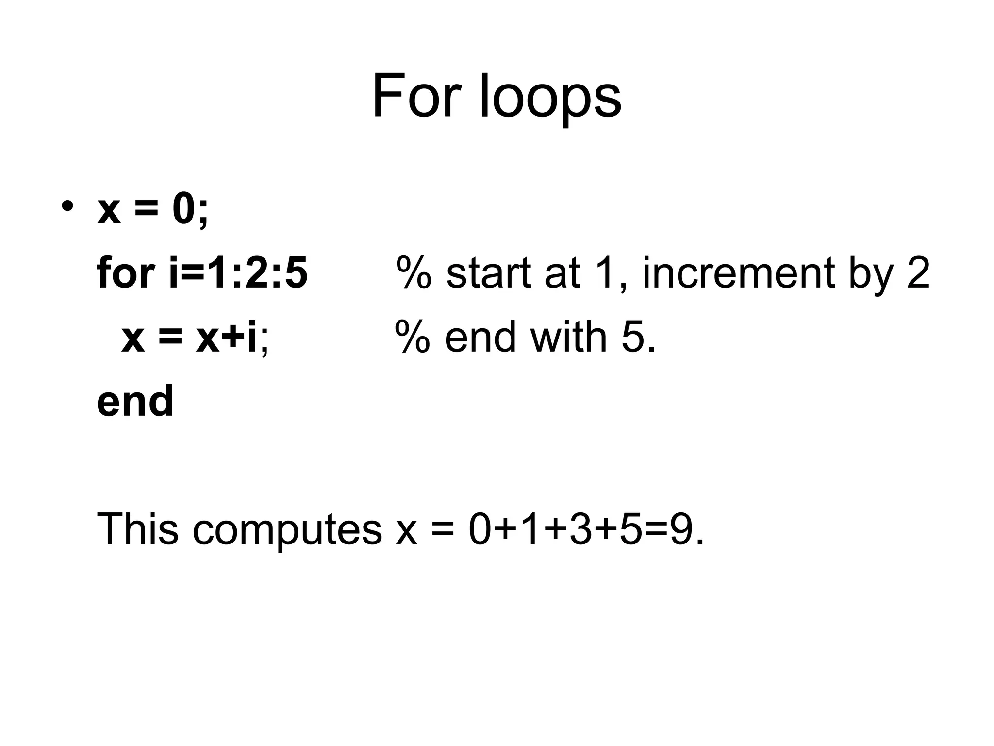
For loops
• x = 0;
for i=1:2:5 % start at 1, increment by 2
x = x+i; % end with 5.
end
This computes x = 0+1+3+5=9.

While loops
• x=7;
while (x > = 0)
x = x-2;
end;
This computes x = 7-2-2-2-2 = -1.

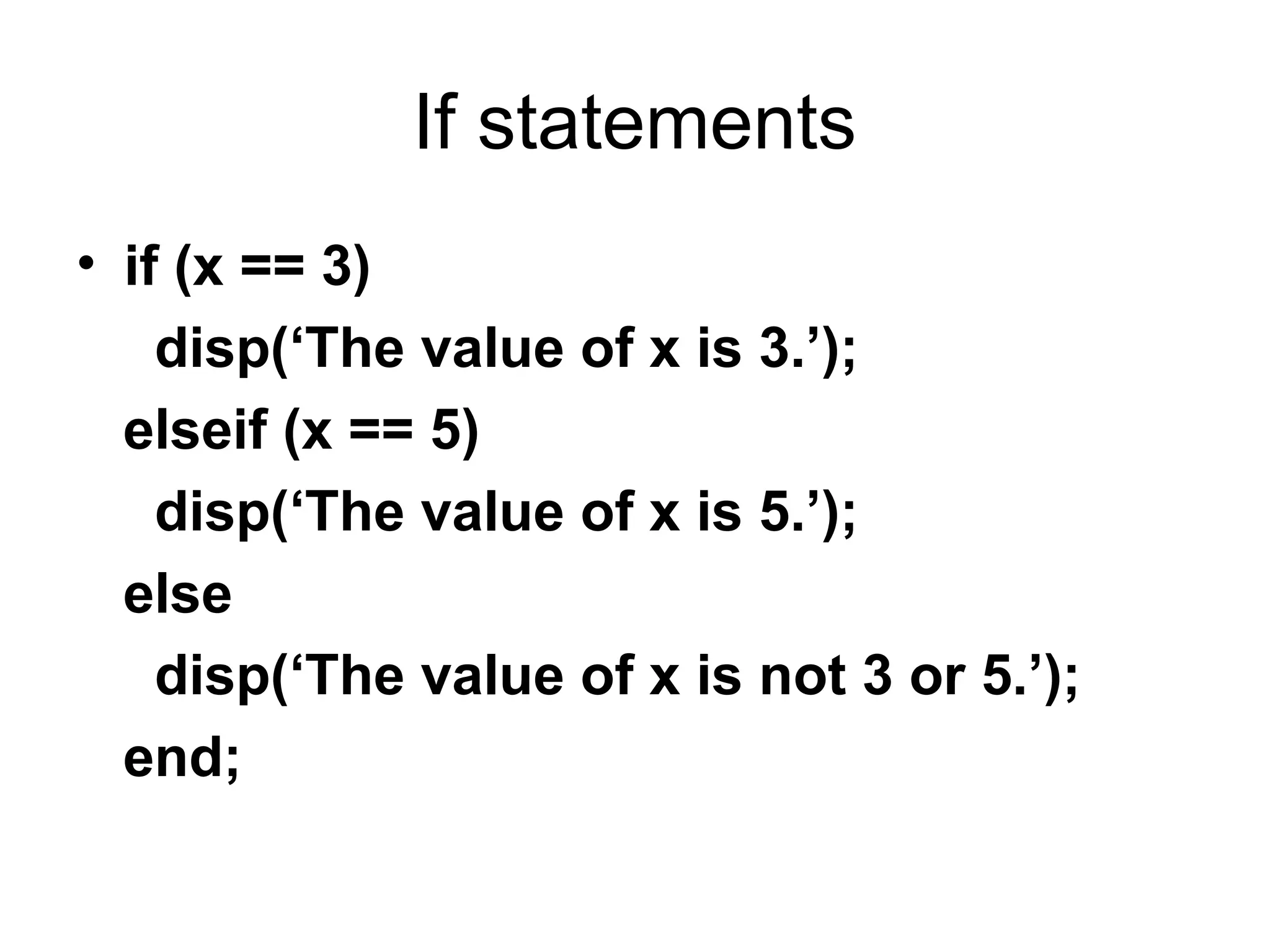
If statements
• if (x == 3)
disp(‘The value of x is 3.’);
elseif (x == 5)
disp(‘The value of x is 5.’);
else
disp(‘The value of x is not 3 or 5.’);
end;

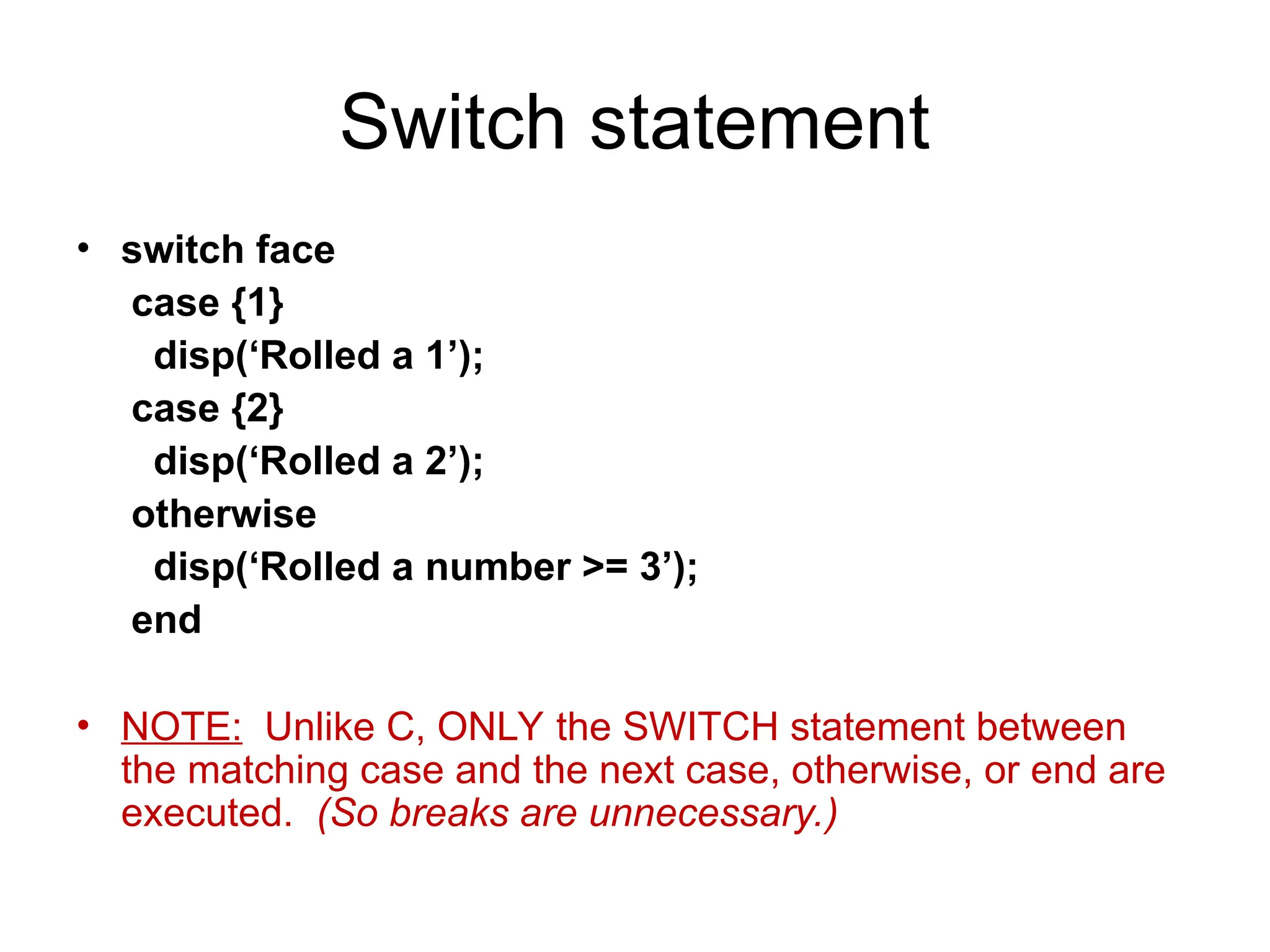
Switch statement
• switch face
case {1}
disp(‘Rolled a 1’);
case {2}
disp(‘Rolled a 2’);
otherwise
disp(‘Rolled a number >= 3’);
end
• NOTE: Unlike C, ONLY the SWITCH statement between
the matching case and the next case, otherwise, or end are
executed. (So breaks are unnecessary.)

Break statements
• break – terminates execution of for and
while loops. For nested loops, it exits the
innermost loop only.

Vectorization
• Because Matlab is an interpreted
language, i.e., it is not compiled before
execution, loops run slowly.
• Vectorized code runs faster in Matlab.
• Example: x=[1 2 3];
for i=1:3 Vectorized:
x(i) = x(i)+5; VS. x = x+5;
end;

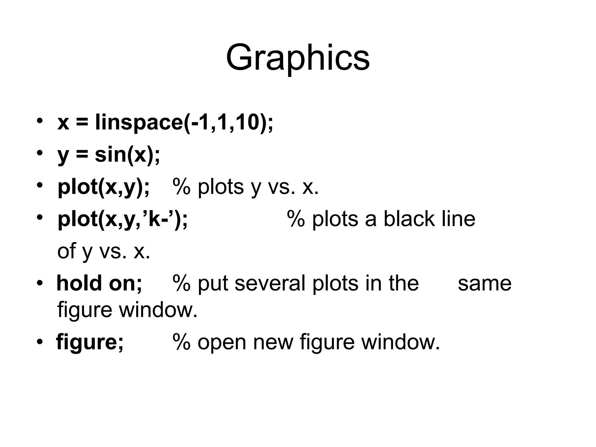
Graphics
• x = linspace(-1,1,10);
• y = sin(x);
• plot(x,y); % plots y vs. x.
• plot(x,y,’k-’); % plots a black line
of y vs. x.
• hold on; % put several plots in the same
figure window.
• figure; % open new figure window.

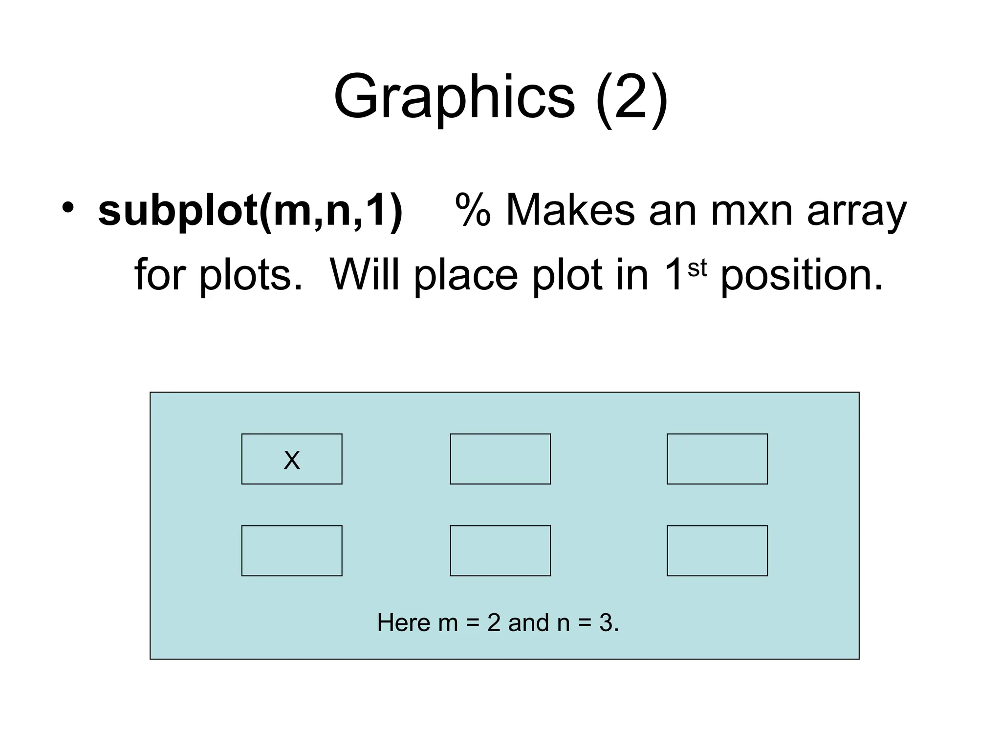
Graphics (2)
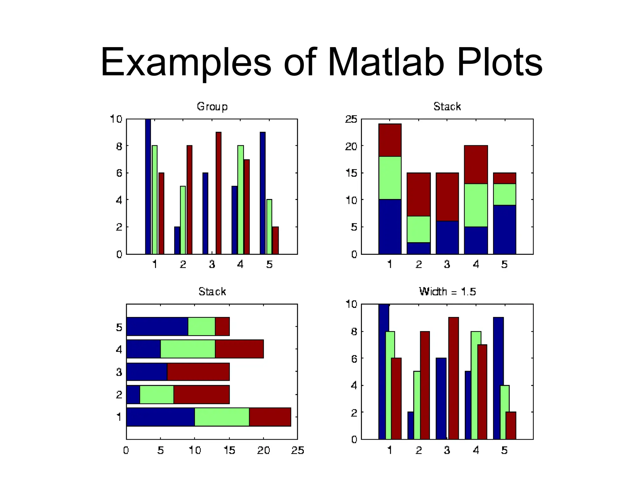
• subplot(m,n,1) % Makes an mxn array
for plots. Will place plot in 1st
position.
X
Here m = 2 and n = 3.

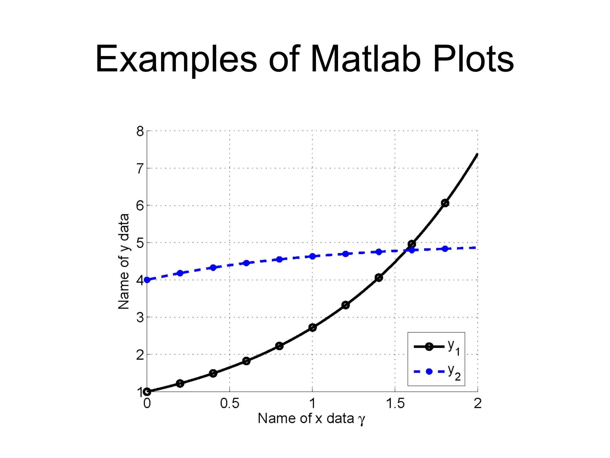
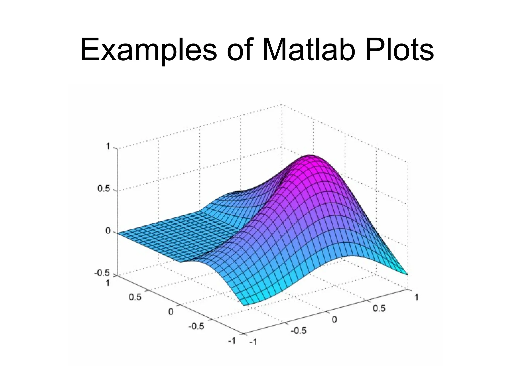
Graphics (3)
• plot3(x,y,z) % plot 2D function.
• mesh(x_ax,y_ax,z_mat) – surface plot.
• contour(z_mat) – contour plot of z.
• axis([xmin xmax ymin ymax]) – change
axes
• title(‘My title’); - add title to figure;
• xlabel, ylabel – label axes.
• legend – add key to figure.

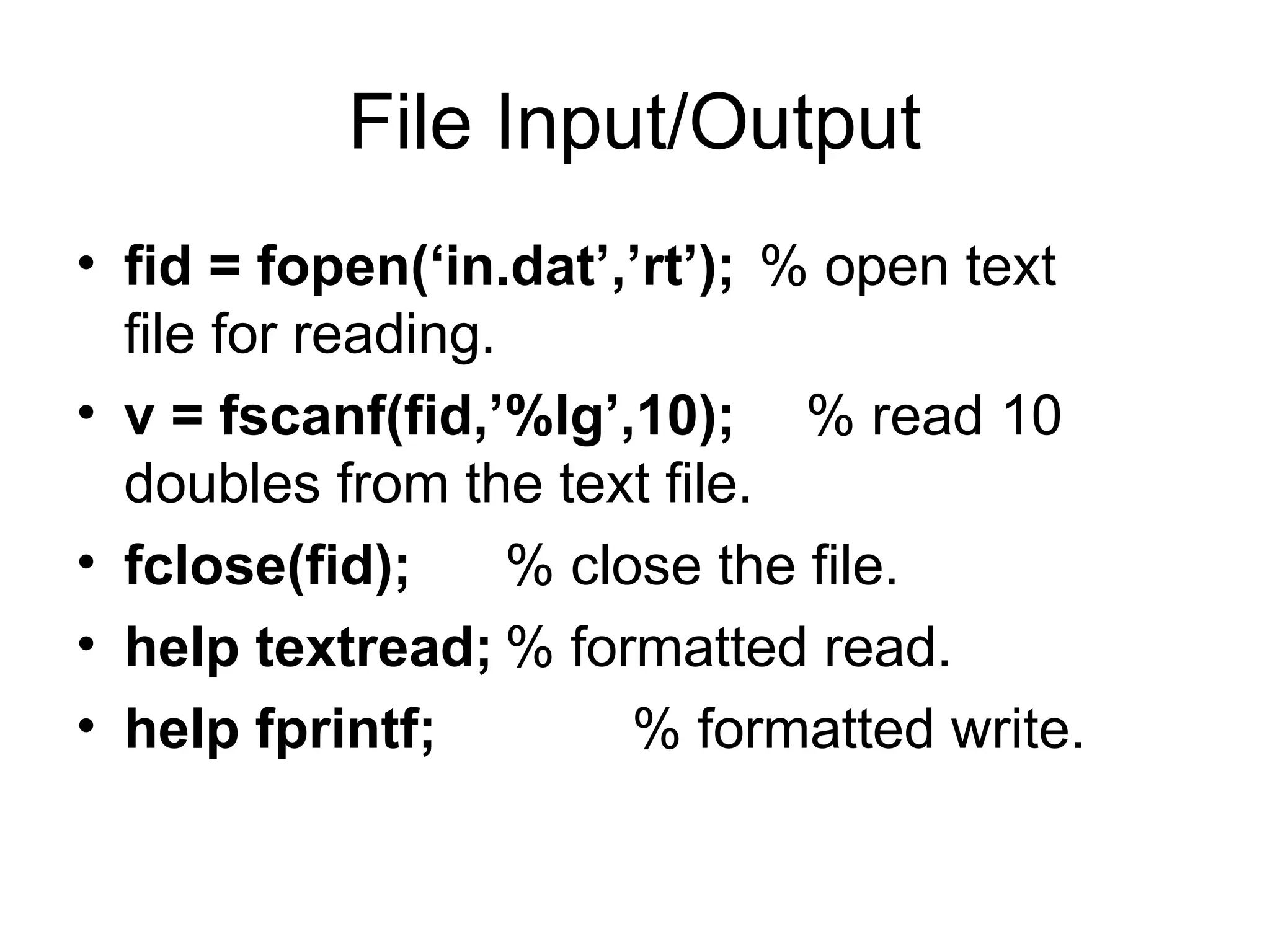
File Input/Output
• fid = fopen(‘in.dat’,’rt’); % open text
file for reading.
• v = fscanf(fid,’%lg’,10); % read 10
doubles from the text file.
• fclose(fid); % close the file.
• help textread; % formatted read.
• help fprintf; % formatted write.

Example Data File
Sally Type1 12.34 45 Yes
Joe Type2 23.54 60 No
Bill Type1 34.90 12 No

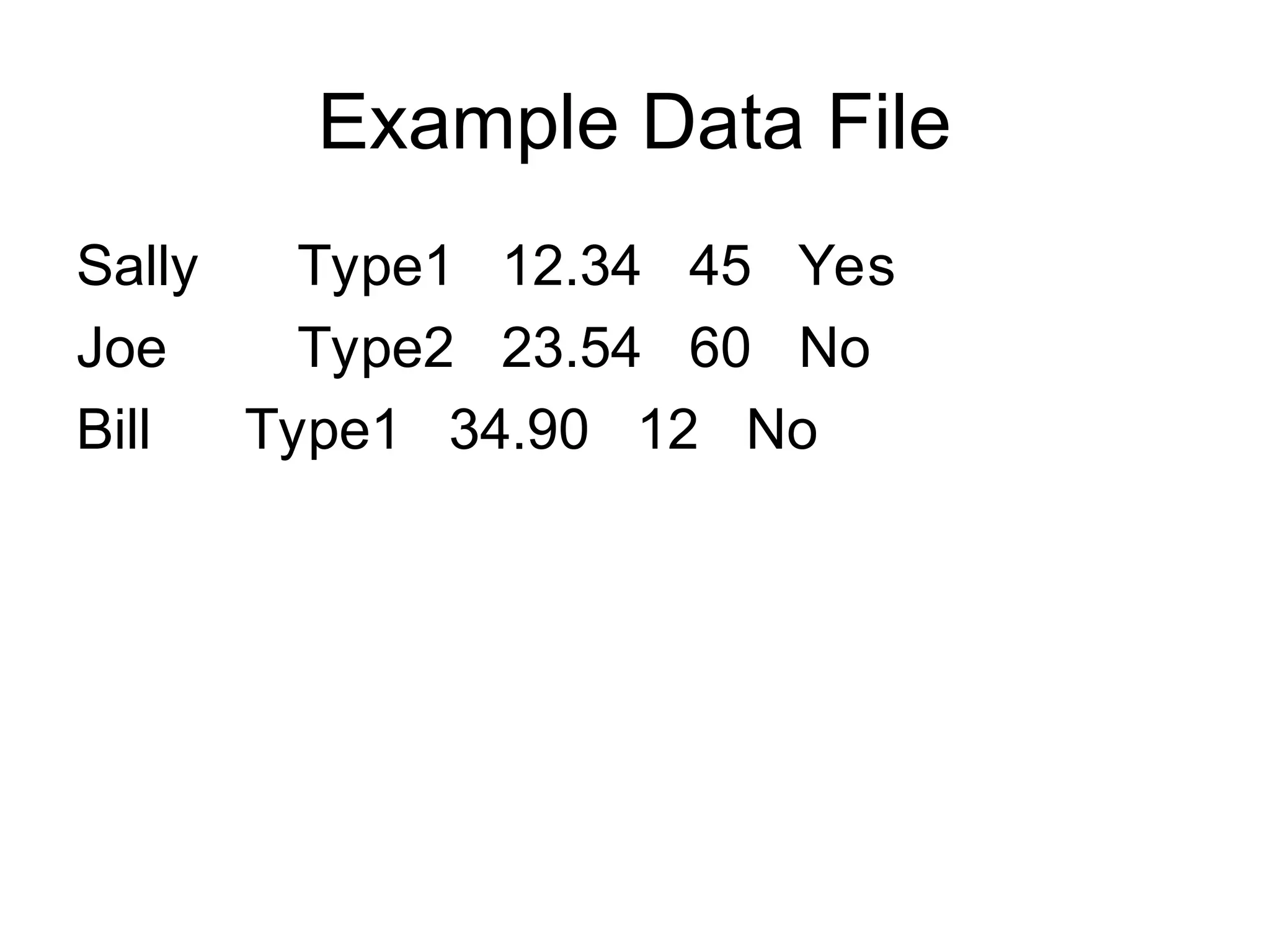
Read Entire Dataset
fid = fopen(‘mydata.dat’, ‘r’); % open file
for reading.
% Read-in data from mydata.dat.
[names,types,x,y,answer] =
textread(fid,’%s%s%f%d%s’);
fclose(fid); % close file.

Read Partial Dataset
for reading.
% Read-in first column of data from mydata.dat.
[names] = textread(fid,’%s %*s %*f %*d %*s’);

Read 1 Line of Data
% for reading.
% Read-in one line of data corresponding
% to Joe’s entry.
[name,type,x,y,answer] =… textread(fid,’%s%s
%f%d%s’,1,…
’headerlines’,1);

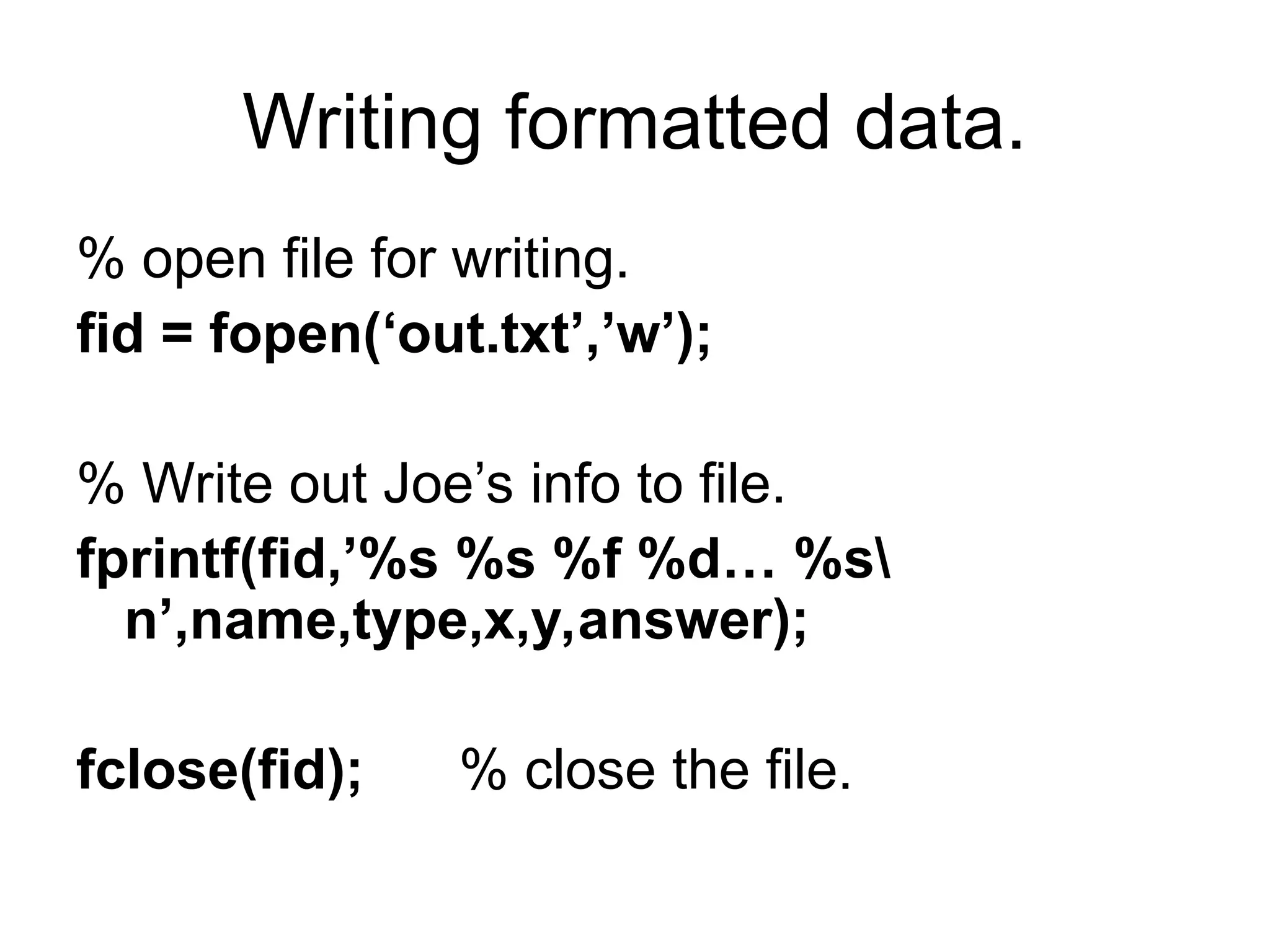
Writing formatted data.
% open file for writing.
fid = fopen(‘out.txt’,’w’);
% Write out Joe’s info to file.
fprintf(fid,’%s %s %f %d… %s
n’,name,type,x,y,answer);
fclose(fid); % close the file.

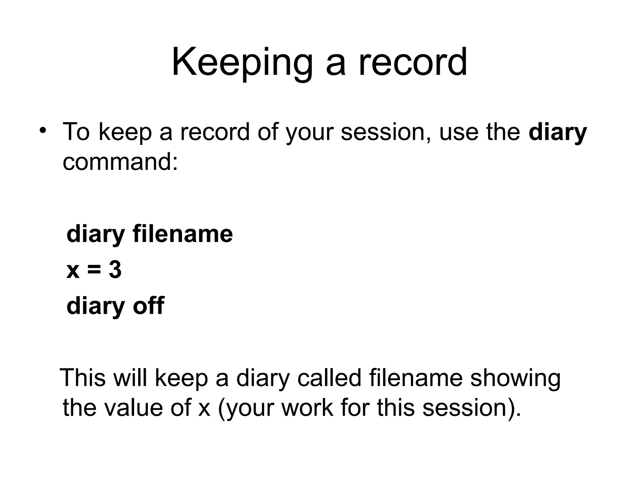
Keeping a record
• To keep a record of your session, use the diary
command:
diary filename
x = 3
diary off
This will keep a diary called filename showing
the value of x (your work for this session).

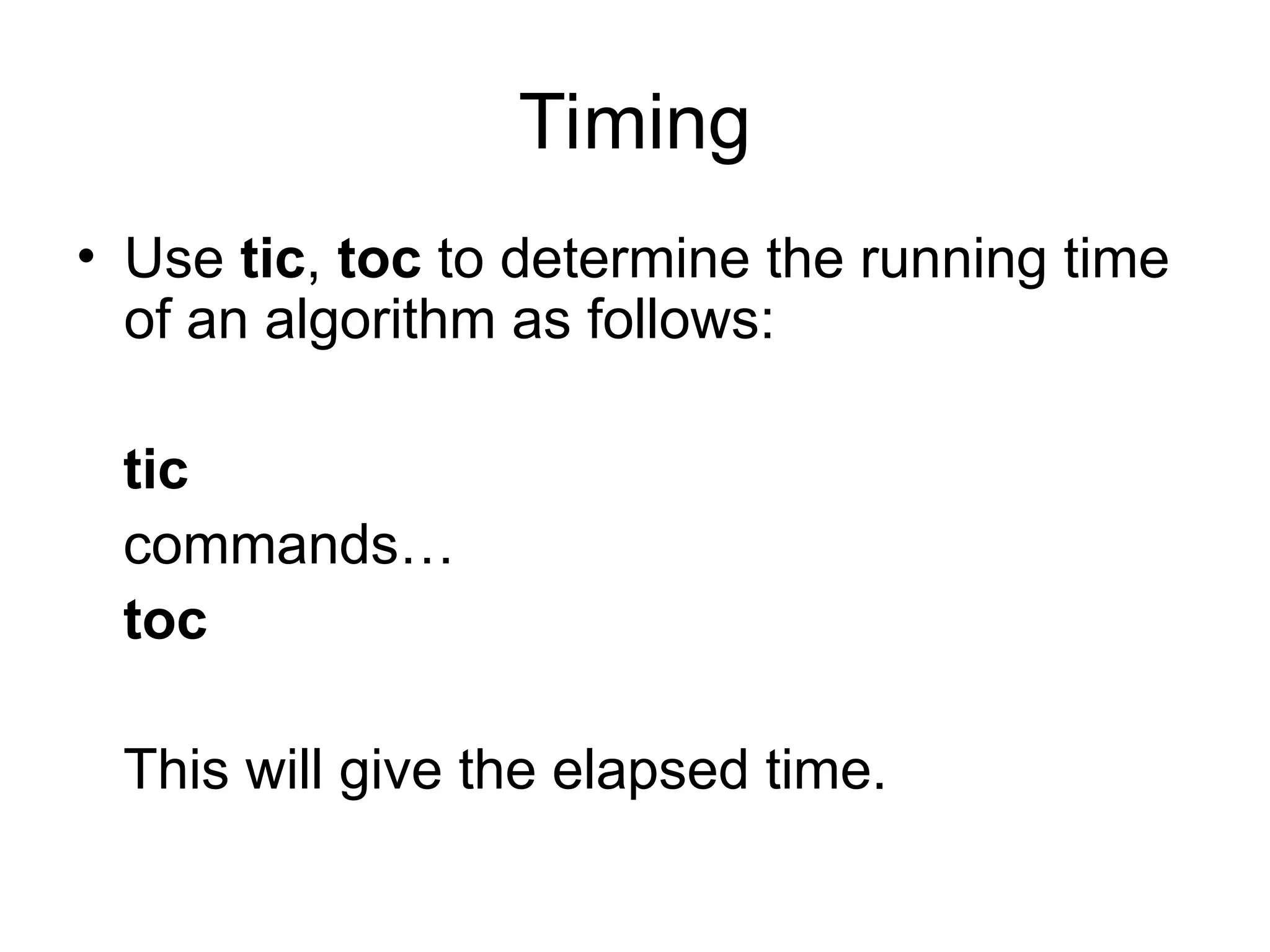
Timing
• Use tic, toc to determine the running time
of an algorithm as follows:
tic
commands…
toc
This will give the elapsed time.

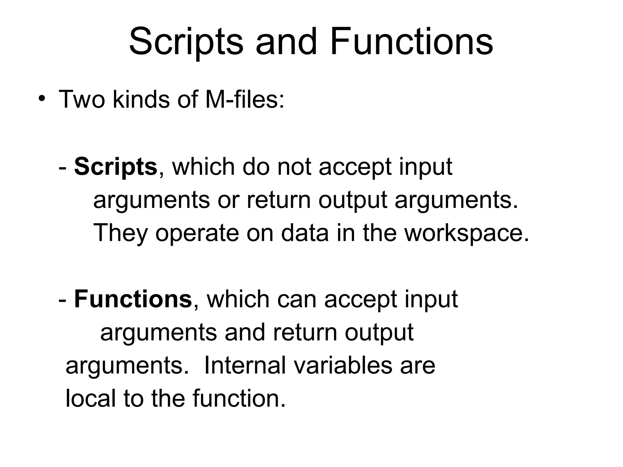
Scripts and Functions
• Two kinds of M-files:
- Scripts, which do not accept input
arguments or return output arguments.
They operate on data in the workspace.
- Functions, which can accept input
arguments and return output
arguments. Internal variables are
local to the function.

M-file functions
• function [area,circum] = circle(r)
% [area, circum] = circle(r) returns the
% area and circumference of a circle
% with radius r.
area = pi*r^2;
circum = 2*pi*r;
• Save function in circle.m.

M-file scripts
• r = 7;
[area,circum] = circle(r);
% call our circle function.
disp([‘The area of a circle having…
radius ‘ num2str(r) ‘ is ‘… num2str(area)]);
• Save the file as myscript.m.

Tutorial sources
• http://docplayer.net/15715694-Introduction
-to-matlab-basics-reference-from-azerniko
v-sergei-mesergei-tx-technion-ac-il.html
• Tutorial by Azernikov Sergei.

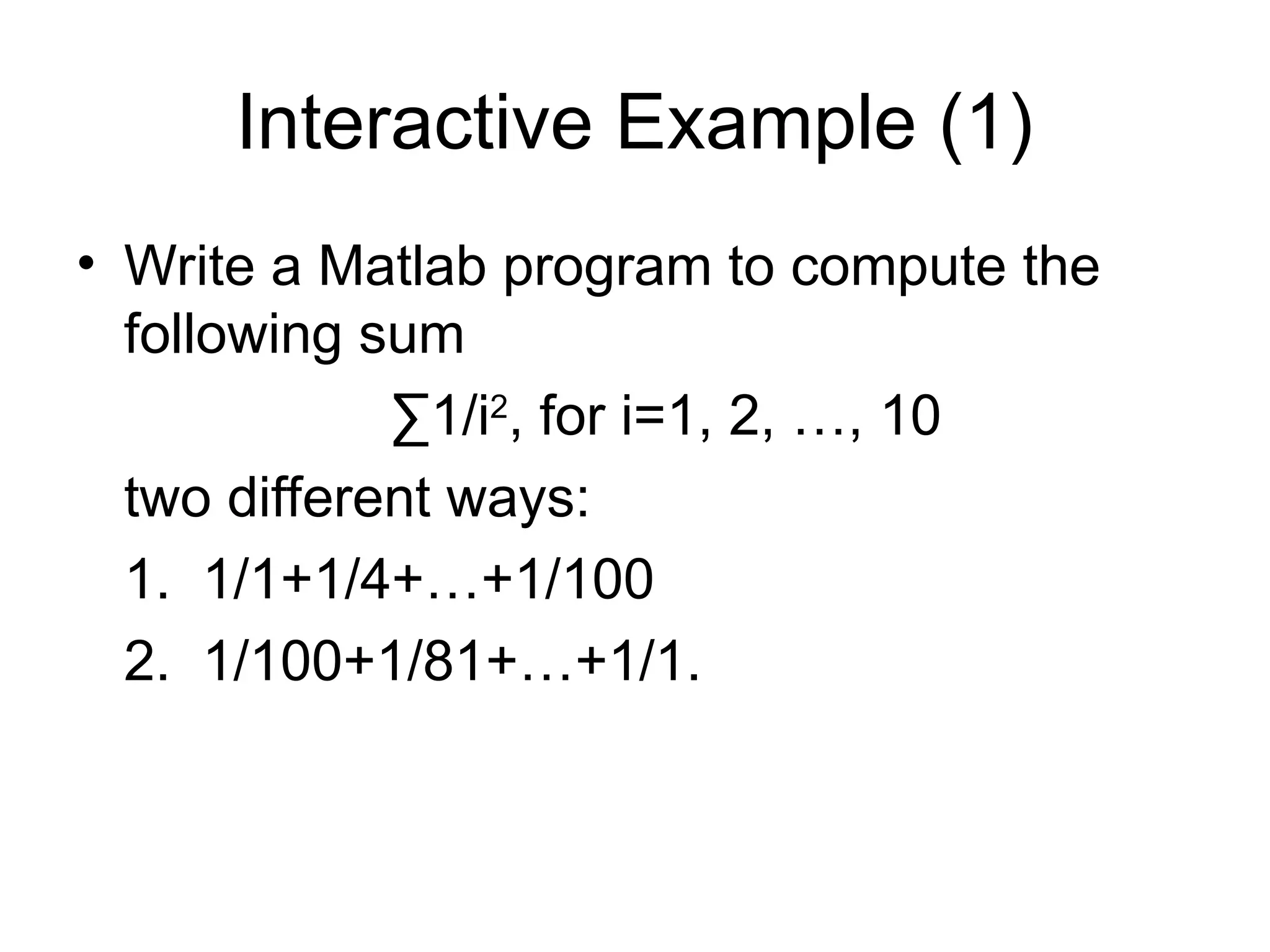
Interactive Example (1)
• Write a Matlab program to compute the
following sum
∑1/i2
, for i=1, 2, …, 10
two different ways:
1. 1/1+1/4+…+1/100
2. 1/100+1/81+…+1/1.

Solution
% Forward summation
forwardsum = 0;
for i=1:10
forwardsum = forwardsum+1/(i^2);
end;
% Backward summation
backwardsum = 0;
for i=10:-1:1
backwardsum = backwardsum+1/(i^2);
end;

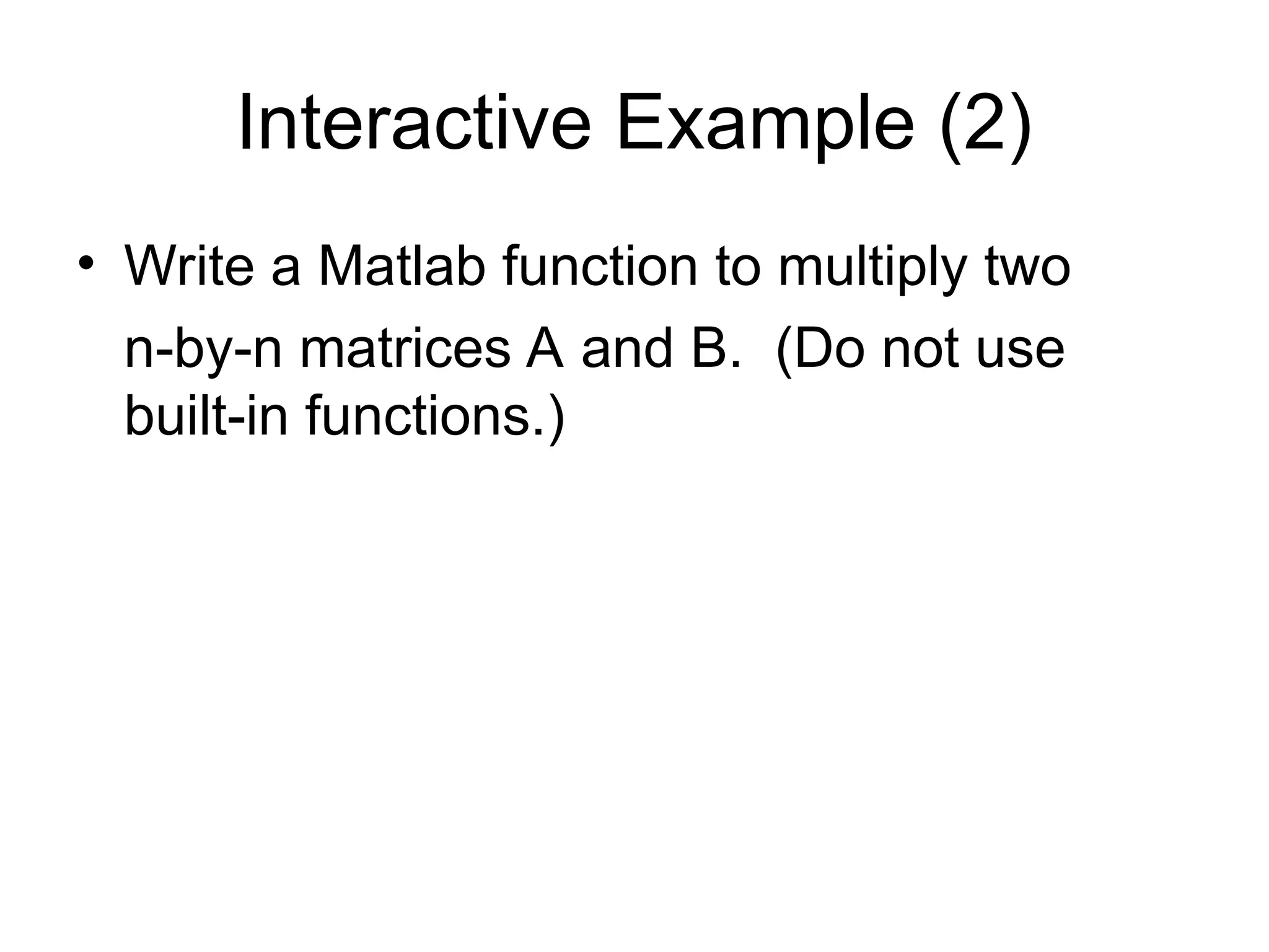
Interactive Example (2)
• Write a Matlab function to multiply two
n-by-n matrices A and B. (Do not use
built-in functions.)

Solution
function [C] = matrix_multiply(A,B,n)
C = zeros(n,n);
for i=1:n
for j=1:n
for k=1:n
C(i,j) = C(i,j) + A(i,k)*B(k,j);
end;
end;
end;
Can this code be written so that it
runs faster?
Hint: Use vectorization.

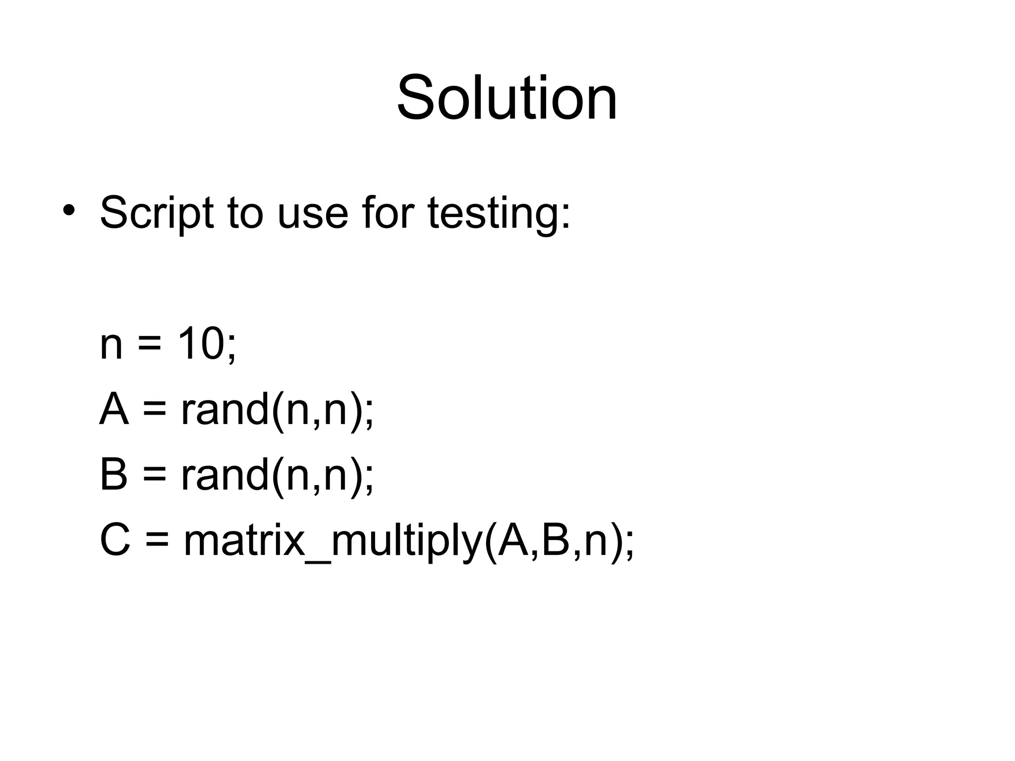
Solution
• Script to use for testing:
n = 10;
A = rand(n,n);
B = rand(n,n);
C = matrix_multiply(A,B,n);

matlab tutorial with separate function description and handson learning

More Related Content

Similar to matlab tutorial with separate function description and handson learning

More from vishalkumarpandey12

Recently uploaded

matlab tutorial with separate function description and handson learning