Download as PDF, PPTX
![Generating Matrices
A scalar can be created in MATLAB as follows:
>> x = 23;
A matrix with only one row is called a row vector. A row vector
can be created in MATLAB as follows (note the commas):
>> y = [12,10,-3]
y =
12 10 -3
A matrix with only one column is called a column vector. A
column vector can be created in MATLAB as follows:
>> z = [12;10;-3]
z =
12
10
-3](https://image.slidesharecdn.com/matlab-140930120808-phpapp01/75/bobok-9-2048.jpg)
![Generating Matrices
MATLAB treats row vector and column vector very differently
A matrix can be created in MATLAB as follows (note the
commas and semicolons)
>> X = [1,2,3;4,5,6;7,8,9]
X =
1 2 3
4 5 6
7 8 9
Matrices must be rectangular!](https://image.slidesharecdn.com/matlab-140930120808-phpapp01/75/bobok-10-2048.jpg)
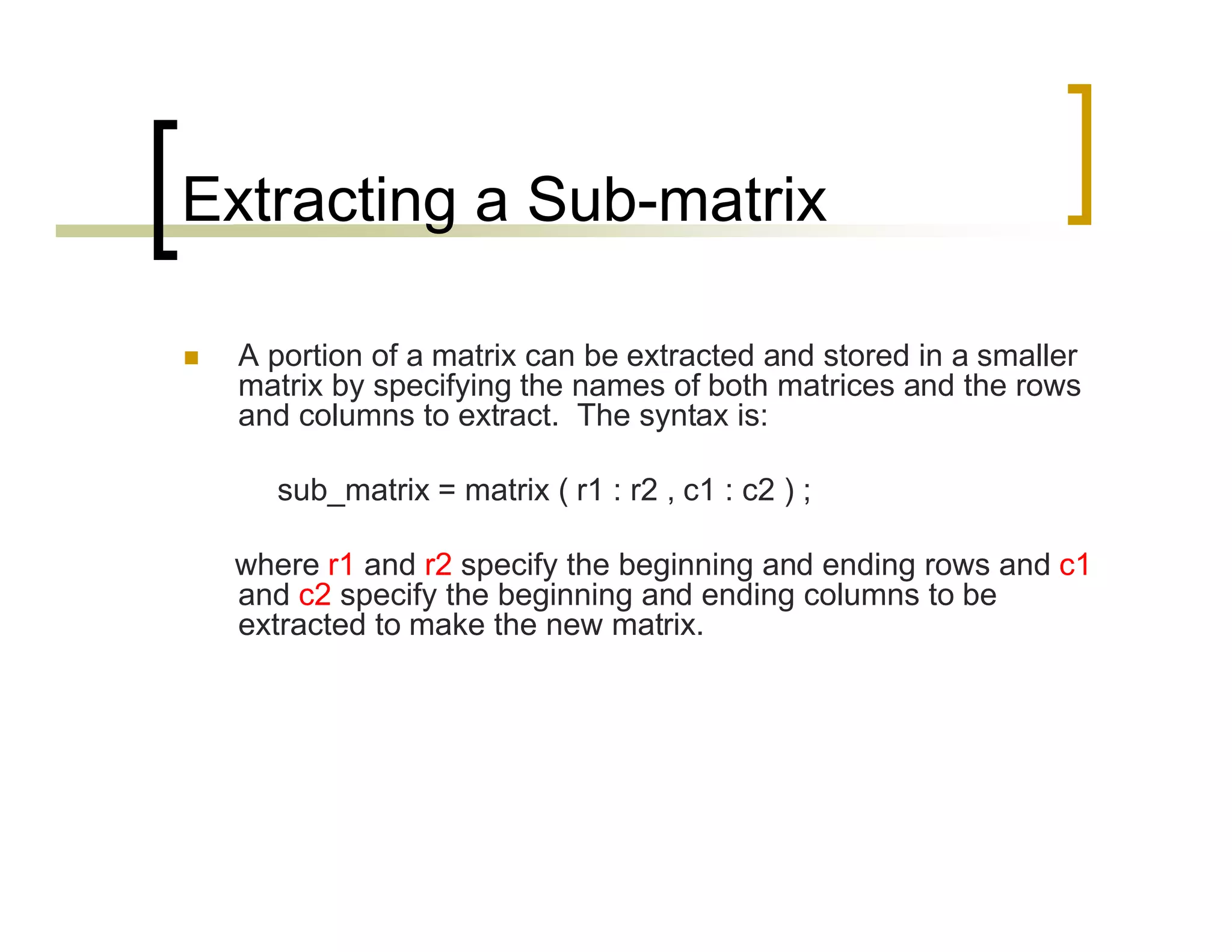
![Extracting a Sub-matrix
Example :
>> X = [1,2,3;4,5,6;7,8,9]
X =
1 2 3
4 5 6
7 8 9
>> X22 = X(1:2 , 2:3)
X22 =
2 3
5 6
>> X13 = X(3,1:3)
X13 =
7 8 9
>> X21 = X(1:2,1)
X21 =
1
4](https://image.slidesharecdn.com/matlab-140930120808-phpapp01/75/bobok-13-2048.jpg)
![Matrix Extension
>> a = [1,2i,0.56]
a =
1 0+2i 0.56
>> a(2,4) = 0.1
a =
1 0+2i 0.56 0
0 0 0 0.1
repmat – replicates and tiles a
matrix
>> b = [1,2;3,4]
b =
1 2
3 4
>> b_rep = repmat(b,1,2)
b_rep =
1 2 1 2
3 4 3 4
Concatenation
>> a = [1,2;3,4]
a =
1 2
3 4
>> a_cat =[a,2*a;3*a,2*a]
a_cat =
1 2 2 4
3 4 6 8
3 6 2 4
9 12 6 8
NOTE: The resulting matrix must
be rectangular](https://image.slidesharecdn.com/matlab-140930120808-phpapp01/75/bobok-14-2048.jpg)
![Matrix Addition
Increment all the elements of
a matrix by a single value
>> x = [1,2;3,4]
x =
1 2
3 4
>> y = x + 5
y =
6 7
8 9
Adding two matrices
>> xsy = x + y
xsy =
7 9
11 13
>> z = [1,0.3]
z =
1 0.3
>> xsz = x + z
??? Error using => plus
Matrix dimensions must
agree](https://image.slidesharecdn.com/matlab-140930120808-phpapp01/75/bobok-15-2048.jpg)
![Matrix Multiplication
Matrix multiplication
>> a = [1,2;3,4]; (2x2)
>> b = [1,1]; (1x2)
>> c = b*a
c =
4 6
>> c = a*b
??? Error using ==> mtimes
Inner matrix dimensions
must agree.
Element wise multiplication
>> a = [1,2;3,4];
>> b = [1,½;1/3,¼];
>> c = a.*b
c =
1 1
1 1](https://image.slidesharecdn.com/matlab-140930120808-phpapp01/75/bobok-16-2048.jpg)
![Matrix Element wise operations
>> a = [1,2;1,3];
>> b = [2,2;2,1];
Element wise division
>> c = a./b
c =
0.5 1
0.5 3
Element wise multiplication
>> c = a.*b
c =
2 4
2 3
Element wise power operation
>> c = a.^2
c =
1 4
1 9
>> c = a.^b
c =
1 4
1 3](https://image.slidesharecdn.com/matlab-140930120808-phpapp01/75/bobok-17-2048.jpg)
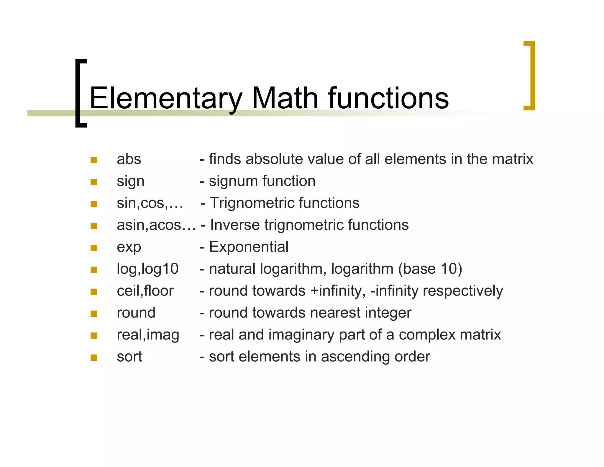
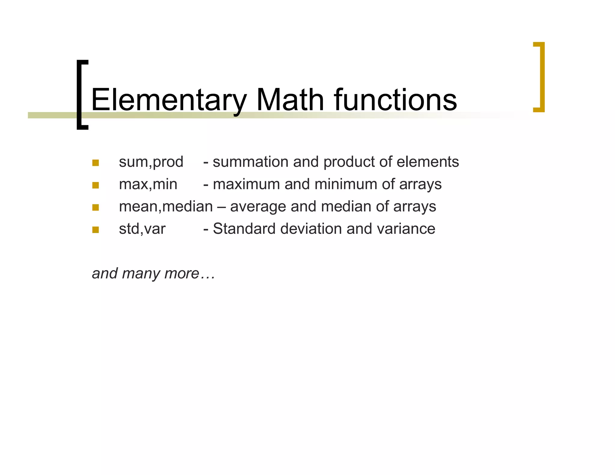
![Matrix Manipulation functions
zeros : creates an array of all zeros, Ex: x = zeros(3,2)
ones : creates an array of all ones, Ex: x = ones(2)
eye : creates an identity matrix, Ex: x = eye(3)
rand : generates uniformly distributed random numbers in [0,1]
diag : Diagonal matrices and diagonal of a matrix
size : returns array dimensions
length : returns length of a vector (row or column)
det : Matrix determinant
inv : matrix inverse
eig : evaluates eigenvalues and eigenvectors
rank : rank of a matrix
find : searches for the given values in an array/matrix.](https://image.slidesharecdn.com/matlab-140930120808-phpapp01/75/bobok-18-2048.jpg)

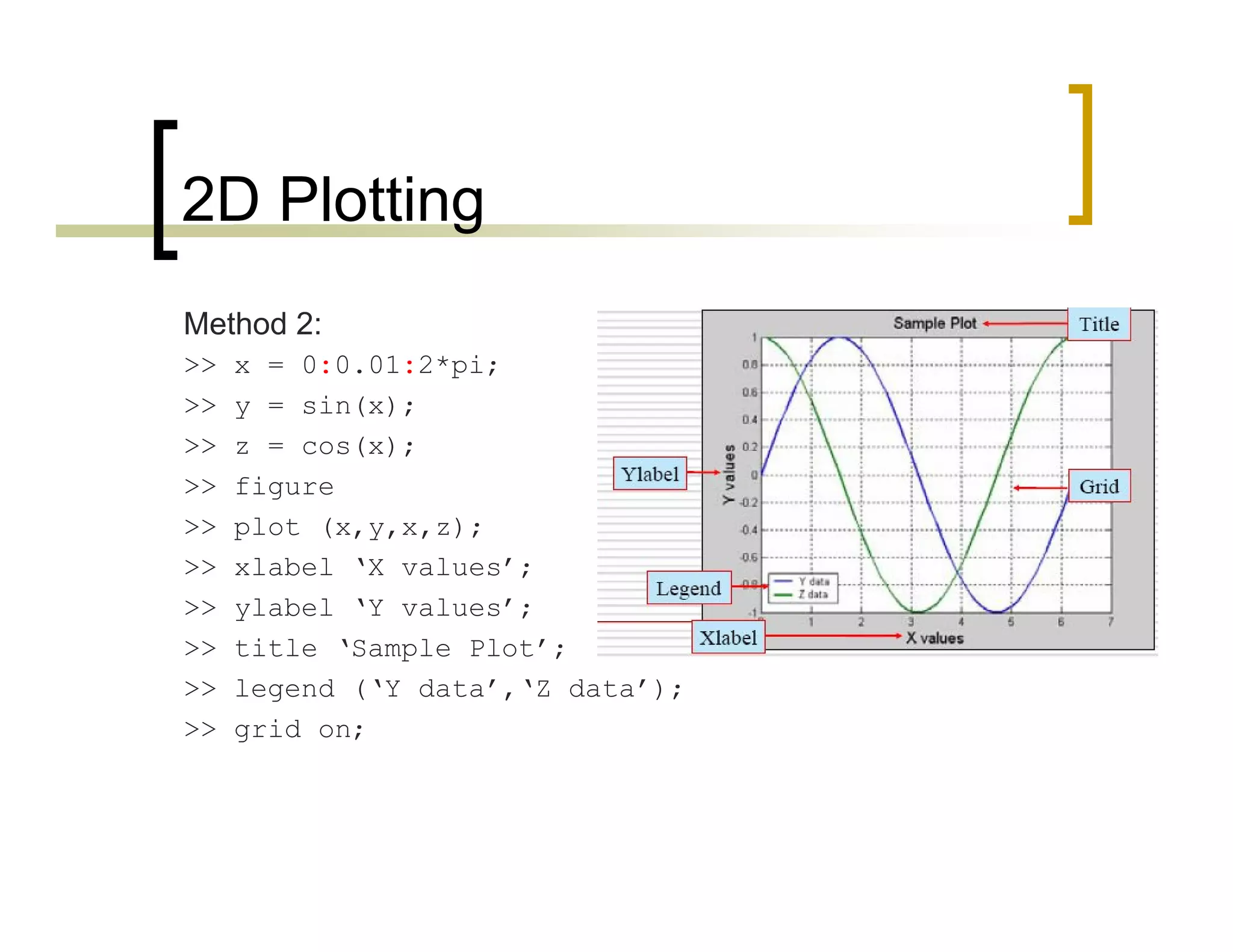
![2D Plotting
Example 1: Plot sin(x) and cos(x) over [0,2π], on the same plot with
different colours
Method 1:
>> x = linspace(0,2*pi,1000);
>> y = sin(x);
>> z = cos(x);
>> hold on;
>> plot(x,y,‘b’);
>> plot(x,z,‘g’);
>> xlabel ‘X values’;
>> ylabel ‘Y values’;
>> title ‘Sample Plot’;
>> legend (‘Y data’,‘Z data’);
>> hold off;](https://image.slidesharecdn.com/matlab-140930120808-phpapp01/75/bobok-23-2048.jpg)
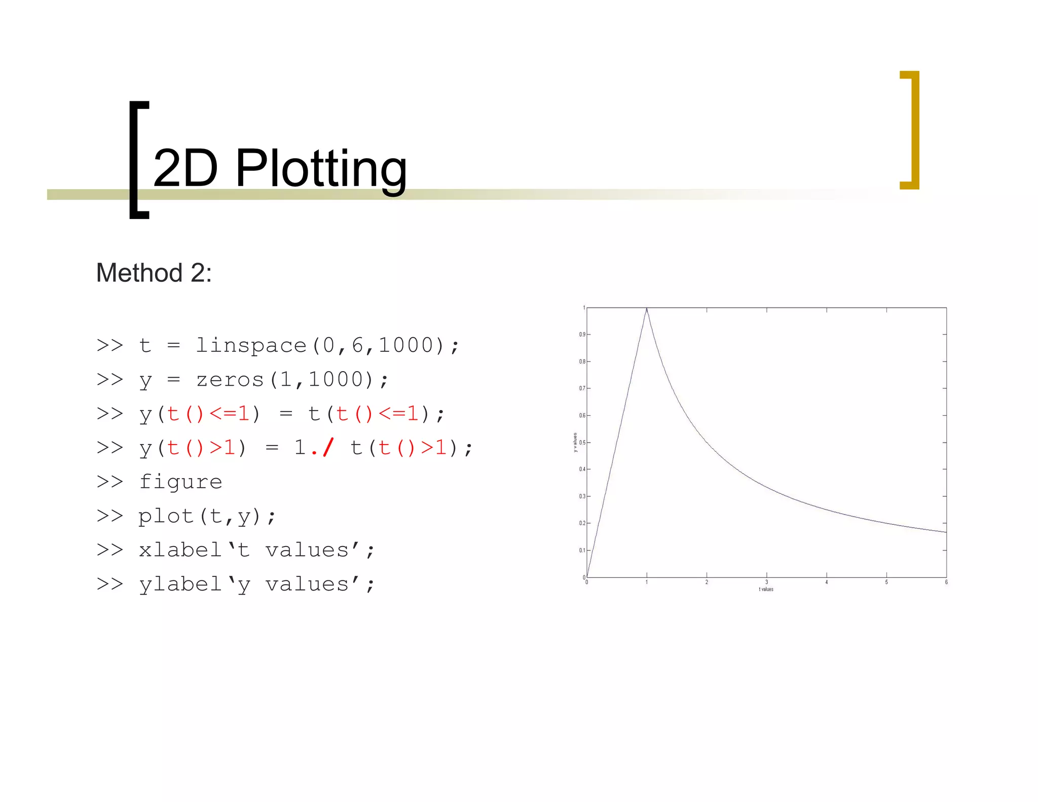
![2D Plotting
Example 2: Plot the following function
t t
Method 1:
>> t1 = linspace(0,1,1000);
>> t2 = linspace(1,6,1000);
>> y1 = t1;
>> y2 = 1./ t2;
>> t = [t1,t2];
>> y = [y1,y2];
>> figure
>> plot(t,y);
>> xlabel ‘t values’, ylabel ‘y values’;
0 1
1/ t 1 t
6
y](https://image.slidesharecdn.com/matlab-140930120808-phpapp01/75/bobok-25-2048.jpg)

![Import/Export from Excel sheet
Copy data from an excel sheet
>> x = xlsread(filename);
% if the file contains numeric values, text and raw data values, then
>> [numeric,txt,raw] = xlsread(filename);
Copy data to an excel sheet
>>x = xlswrite('c:matlabworkdata.xls',A,'A2:C4')
% will write A to the workbook file, data.xls, and attempt to fit the
elements of A into the rectangular worksheet region, A2:C4. On
success, ‘x’ will contain ‘1’, while on failure, ‘x’ will contain ‘0’.
for more information, type help xlswrite at command prompt](https://image.slidesharecdn.com/matlab-140930120808-phpapp01/75/bobok-30-2048.jpg)

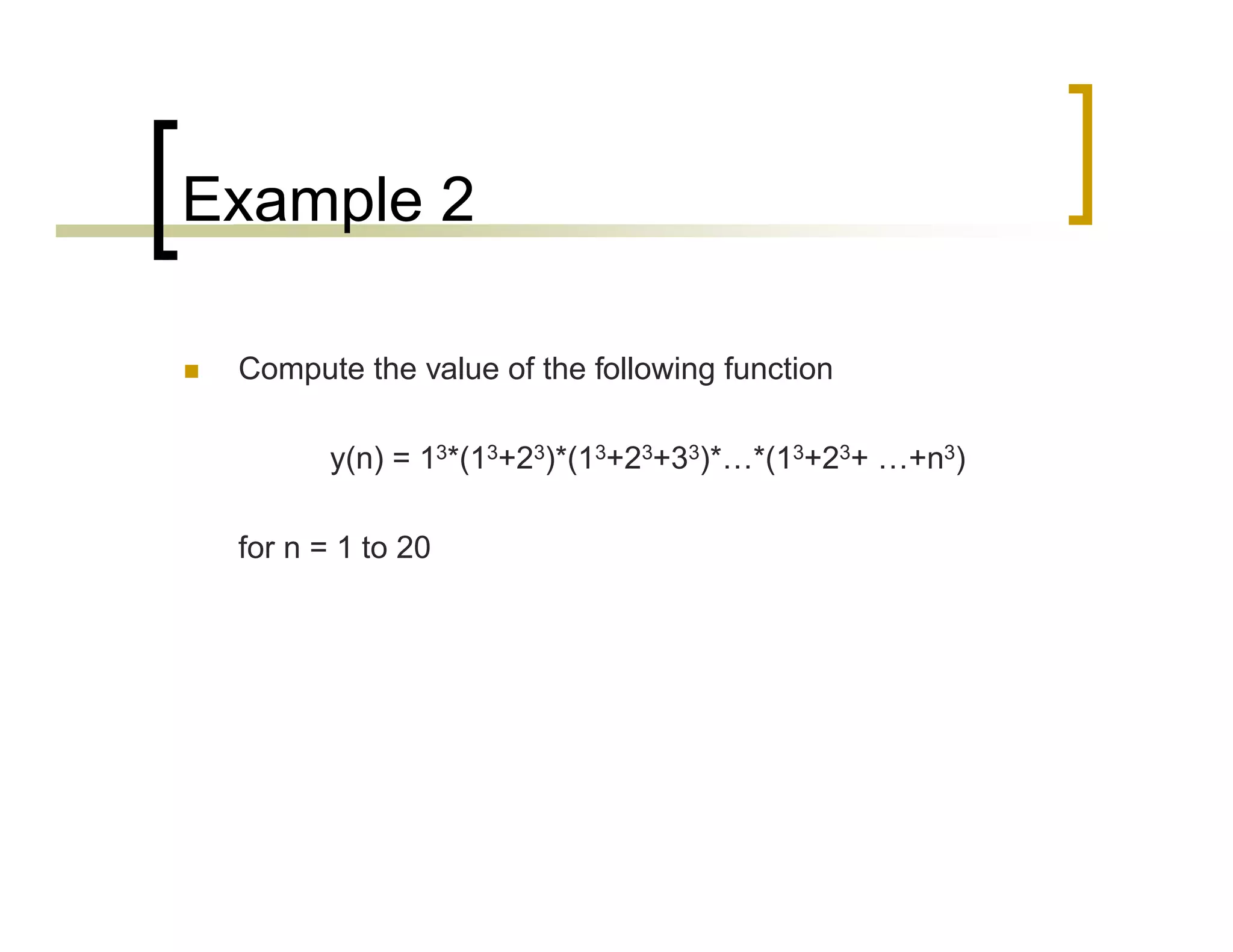
![Example 1
Let x[n] be the input to a non causal FIR filter, with filter
coefficients h[n]. Assume both the input values and the filter
coefficients are stored in column vectors x,h and are given to
you. Compute the output values y[n] for n = 1,2,3 where
19
y n h k x n k
[ ] [ ] [ ]
0
k](https://image.slidesharecdn.com/matlab-140930120808-phpapp01/75/bobok-41-2048.jpg)
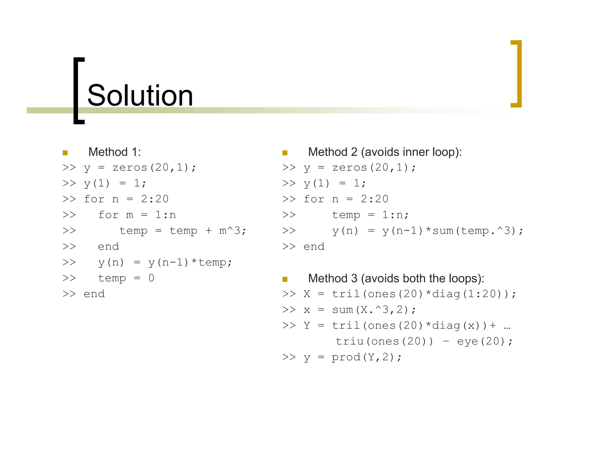
![Solution
Method 1:
>> y = zeros(1,3);
>> for n = 1:3
>> for k = 0:19
>> y(n)= y(n)+h(k)*x(n+k);
>> end
>> end
Method 2 (avoids inner loop):
>> y = zeros(1,3);
>> for n = 1:3
>> y(n) = h’*x(n:(n+19));
>> end
Method 3 (avoids both the loops):
>> X= [x(1:20),x(2:21),x(3:22)];
>> y = h’*X;](https://image.slidesharecdn.com/matlab-140930120808-phpapp01/75/bobok-42-2048.jpg)


![Generating Matrices
A scalar can be created in MATLAB as follows:
>> x = 23;
A matrix with only one row is called a row vector. A row vector
can be created in MATLAB as follows (note the commas):
>> y = [12,10,-3]
y =
12 10 -3
A matrix with only one column is called a column vector. A
column vector can be created in MATLAB as follows:
>> z = [12;10;-3]
z =
12
10
-3](https://crownmelresort.com/image.slidesharecdn.com/matlab-140930120808-phpapp01/75/bobok-9-2048.jpg)
![Generating Matrices
MATLAB treats row vector and column vector very differently
A matrix can be created in MATLAB as follows (note the
commas and semicolons)
>> X = [1,2,3;4,5,6;7,8,9]
X =
1 2 3
4 5 6
7 8 9
Matrices must be rectangular!](https://crownmelresort.com/image.slidesharecdn.com/matlab-140930120808-phpapp01/75/bobok-10-2048.jpg)


![Extracting a Sub-matrix
Example :
>> X = [1,2,3;4,5,6;7,8,9]
X =
1 2 3
4 5 6
7 8 9
>> X22 = X(1:2 , 2:3)
X22 =
2 3
5 6
>> X13 = X(3,1:3)
X13 =
7 8 9
>> X21 = X(1:2,1)
X21 =
1
4](https://crownmelresort.com/image.slidesharecdn.com/matlab-140930120808-phpapp01/75/bobok-13-2048.jpg)
![Matrix Extension
>> a = [1,2i,0.56]
a =
1 0+2i 0.56
>> a(2,4) = 0.1
a =
1 0+2i 0.56 0
0 0 0 0.1
repmat – replicates and tiles a
matrix
>> b = [1,2;3,4]
b =
1 2
3 4
>> b_rep = repmat(b,1,2)
b_rep =
1 2 1 2
3 4 3 4
Concatenation
>> a = [1,2;3,4]
a =
1 2
3 4
>> a_cat =[a,2*a;3*a,2*a]
a_cat =
1 2 2 4
3 4 6 8
3 6 2 4
9 12 6 8
NOTE: The resulting matrix must
be rectangular](https://crownmelresort.com/image.slidesharecdn.com/matlab-140930120808-phpapp01/75/bobok-14-2048.jpg)
![Matrix Addition
Increment all the elements of
a matrix by a single value
>> x = [1,2;3,4]
x =
1 2
3 4
>> y = x + 5
y =
6 7
8 9
Adding two matrices
>> xsy = x + y
xsy =
7 9
11 13
>> z = [1,0.3]
z =
1 0.3
>> xsz = x + z
??? Error using => plus
Matrix dimensions must
agree](https://crownmelresort.com/image.slidesharecdn.com/matlab-140930120808-phpapp01/75/bobok-15-2048.jpg)
![Matrix Multiplication
Matrix multiplication
>> a = [1,2;3,4]; (2x2)
>> b = [1,1]; (1x2)
>> c = b*a
c =
4 6
>> c = a*b
??? Error using ==> mtimes
Inner matrix dimensions
must agree.
Element wise multiplication
>> a = [1,2;3,4];
>> b = [1,½;1/3,¼];
>> c = a.*b
c =
1 1
1 1](https://crownmelresort.com/image.slidesharecdn.com/matlab-140930120808-phpapp01/75/bobok-16-2048.jpg)
![Matrix Element wise operations
>> a = [1,2;1,3];
>> b = [2,2;2,1];
Element wise division
>> c = a./b
c =
0.5 1
0.5 3
Element wise multiplication
>> c = a.*b
c =
2 4
2 3
Element wise power operation
>> c = a.^2
c =
1 4
1 9
>> c = a.^b
c =
1 4
1 3](https://crownmelresort.com/image.slidesharecdn.com/matlab-140930120808-phpapp01/75/bobok-17-2048.jpg)
![Matrix Manipulation functions
zeros : creates an array of all zeros, Ex: x = zeros(3,2)
ones : creates an array of all ones, Ex: x = ones(2)
eye : creates an identity matrix, Ex: x = eye(3)
rand : generates uniformly distributed random numbers in [0,1]
diag : Diagonal matrices and diagonal of a matrix
size : returns array dimensions
length : returns length of a vector (row or column)
det : Matrix determinant
inv : matrix inverse
eig : evaluates eigenvalues and eigenvectors
rank : rank of a matrix
find : searches for the given values in an array/matrix.](https://crownmelresort.com/image.slidesharecdn.com/matlab-140930120808-phpapp01/75/bobok-18-2048.jpg)


![2D Plotting
Example 1: Plot sin(x) and cos(x) over [0,2π], on the same plot with
different colours
Method 1:
>> x = linspace(0,2*pi,1000);
>> y = sin(x);
>> z = cos(x);
>> hold on;
>> plot(x,y,‘b’);
>> plot(x,z,‘g’);
>> xlabel ‘X values’;
>> ylabel ‘Y values’;
>> title ‘Sample Plot’;
>> legend (‘Y data’,‘Z data’);
>> hold off;](https://crownmelresort.com/image.slidesharecdn.com/matlab-140930120808-phpapp01/75/bobok-23-2048.jpg)

![2D Plotting
Example 2: Plot the following function
t t
Method 1:
>> t1 = linspace(0,1,1000);
>> t2 = linspace(1,6,1000);
>> y1 = t1;
>> y2 = 1./ t2;
>> t = [t1,t2];
>> y = [y1,y2];
>> figure
>> plot(t,y);
>> xlabel ‘t values’, ylabel ‘y values’;
0 1
1/ t 1 t
6
y](https://crownmelresort.com/image.slidesharecdn.com/matlab-140930120808-phpapp01/75/bobok-25-2048.jpg)


![Import/Export from Excel sheet
Copy data from an excel sheet
>> x = xlsread(filename);
% if the file contains numeric values, text and raw data values, then
>> [numeric,txt,raw] = xlsread(filename);
Copy data to an excel sheet
>>x = xlswrite('c:matlabworkdata.xls',A,'A2:C4')
% will write A to the workbook file, data.xls, and attempt to fit the
elements of A into the rectangular worksheet region, A2:C4. On
success, ‘x’ will contain ‘1’, while on failure, ‘x’ will contain ‘0’.
for more information, type help xlswrite at command prompt](https://crownmelresort.com/image.slidesharecdn.com/matlab-140930120808-phpapp01/75/bobok-30-2048.jpg)


![Example 1
Let x[n] be the input to a non causal FIR filter, with filter
coefficients h[n]. Assume both the input values and the filter
coefficients are stored in column vectors x,h and are given to
you. Compute the output values y[n] for n = 1,2,3 where
19
y n h k x n k
[ ] [ ] [ ]
0
k](https://crownmelresort.com/image.slidesharecdn.com/matlab-140930120808-phpapp01/75/bobok-41-2048.jpg)
![Solution
Method 1:
>> y = zeros(1,3);
>> for n = 1:3
>> for k = 0:19
>> y(n)= y(n)+h(k)*x(n+k);
>> end
>> end
Method 2 (avoids inner loop):
>> y = zeros(1,3);
>> for n = 1:3
>> y(n) = h’*x(n:(n+19));
>> end
Method 3 (avoids both the loops):
>> X= [x(1:20),x(2:21),x(3:22)];
>> y = h’*X;](https://crownmelresort.com/image.slidesharecdn.com/matlab-140930120808-phpapp01/75/bobok-42-2048.jpg)


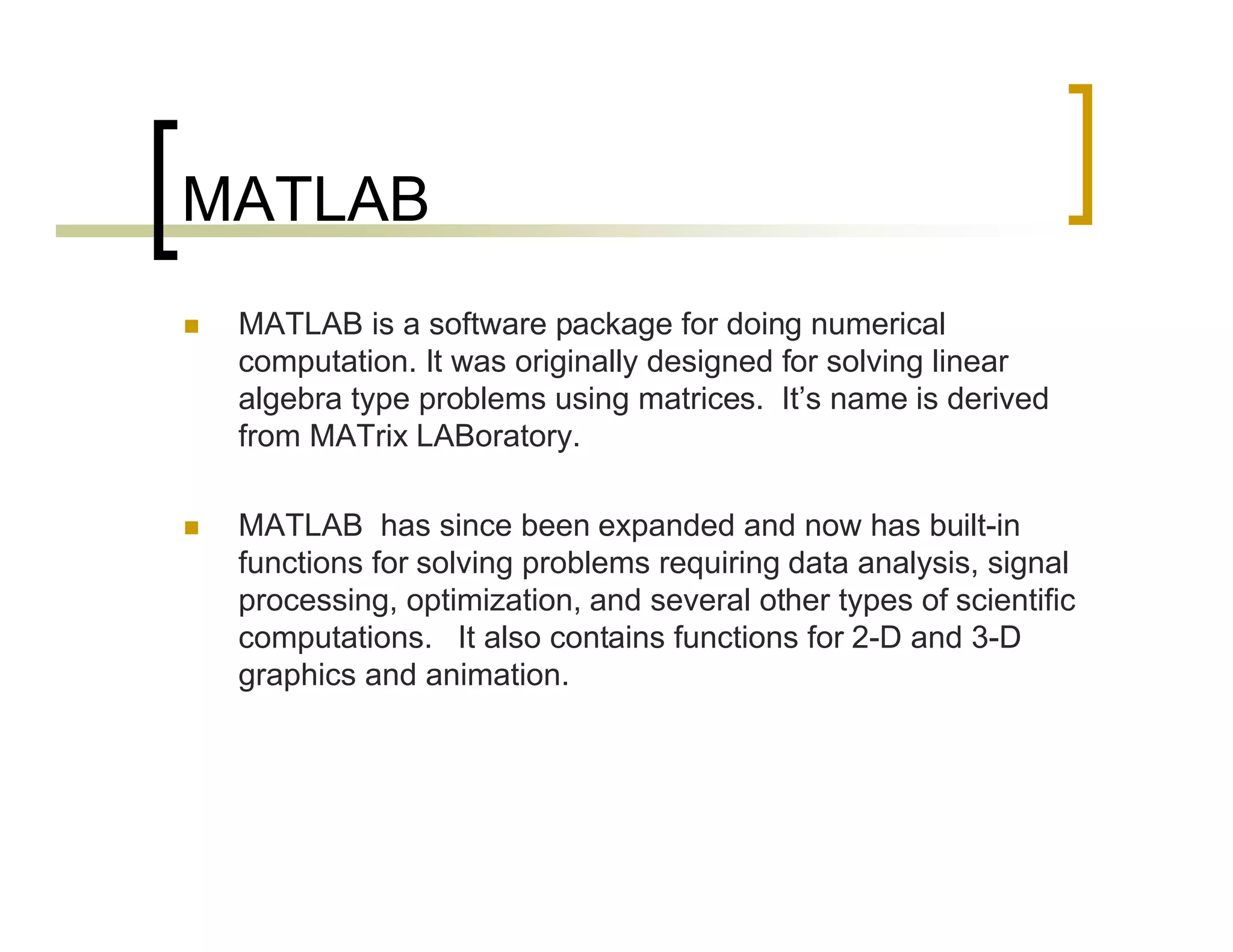
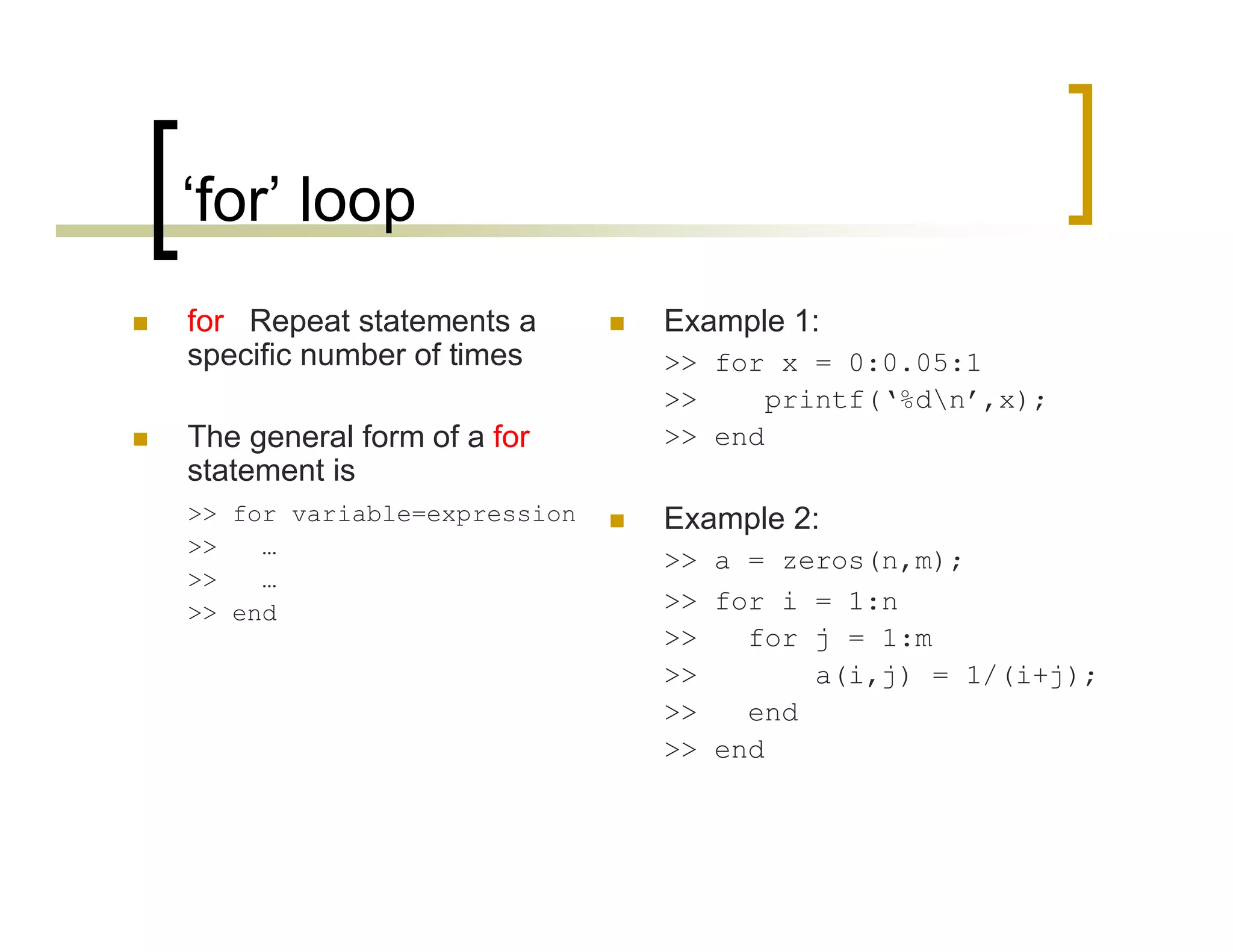
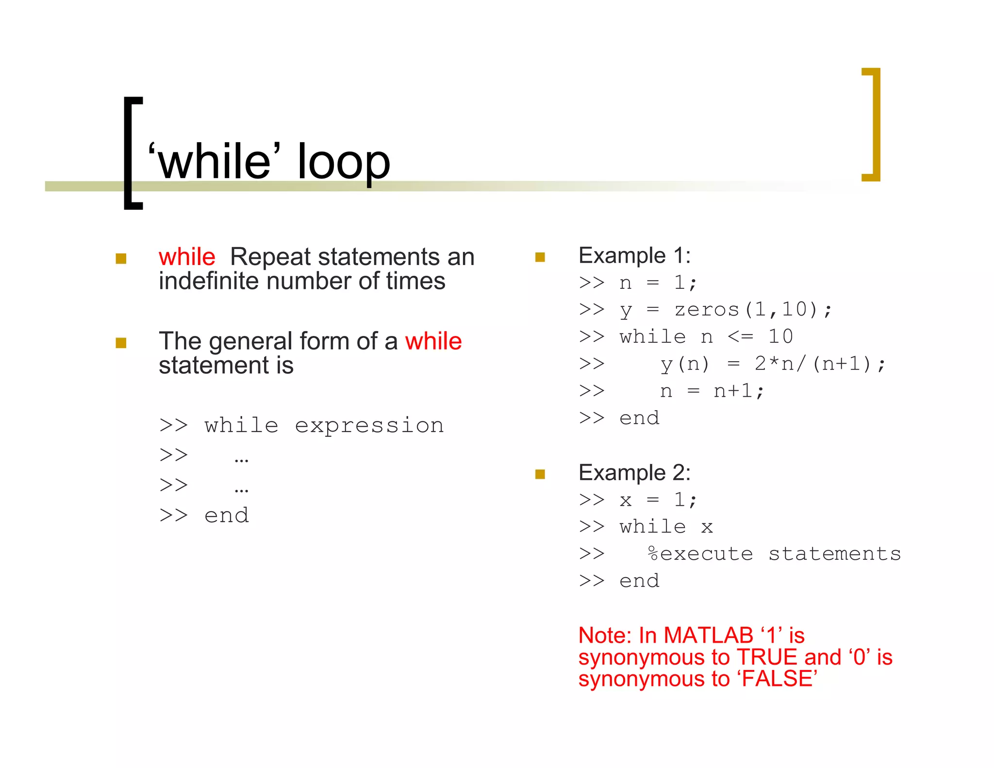
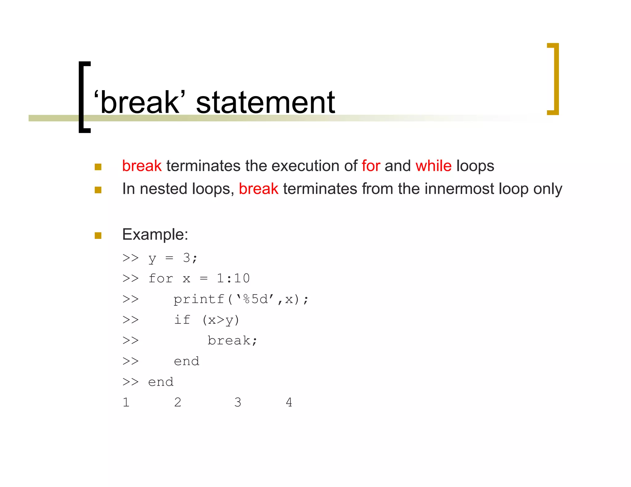
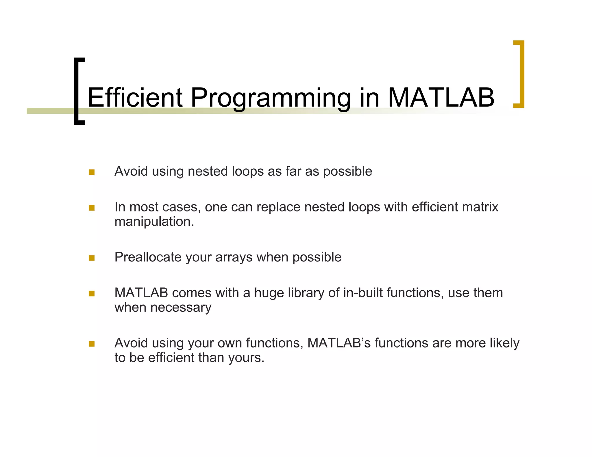
This document provides an overview of MATLAB, including: - MATLAB is a software package for numerical computation, originally designed for linear algebra problems using matrices. It has since expanded to include other scientific computations. - MATLAB treats all variables as matrices and supports various matrix operations like addition, multiplication, element-wise operations, and matrix manipulation functions. - MATLAB allows plotting of 2D and 3D graphics, importing/exporting of data from files and Excel, and includes flow control statements like if/else, for loops, and while loops to structure code execution. - Efficient MATLAB programming involves using built-in functions instead of custom functions, preallocating arrays, and avoiding nested loops where possible through matrix operations.


![Reduction of multiple subsystem [compatibility mode]](https://cdn.slidesharecdn.com/ss_thumbnails/reductionofmultiplesubsystemcompatibilitymode-110418075355-phpapp01-thumbnail.jpg?width=640&height=640&fit=bounds)