Downloaded 146 times
![Polynomials in MATLAB
MATLAB provides a number of functions for the
manipulation of polynomials. These include,
Evaluation of polynomials
Finding roots of polynomials
Addition, subtraction, multiplication, and division of polynomials
Dealing with rational expressions of polynomials
Curve fitting
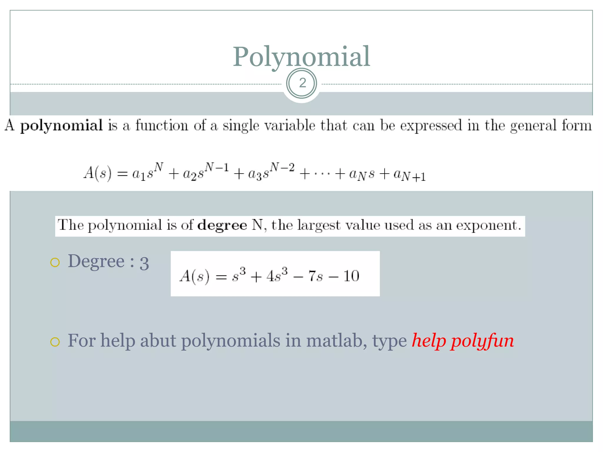
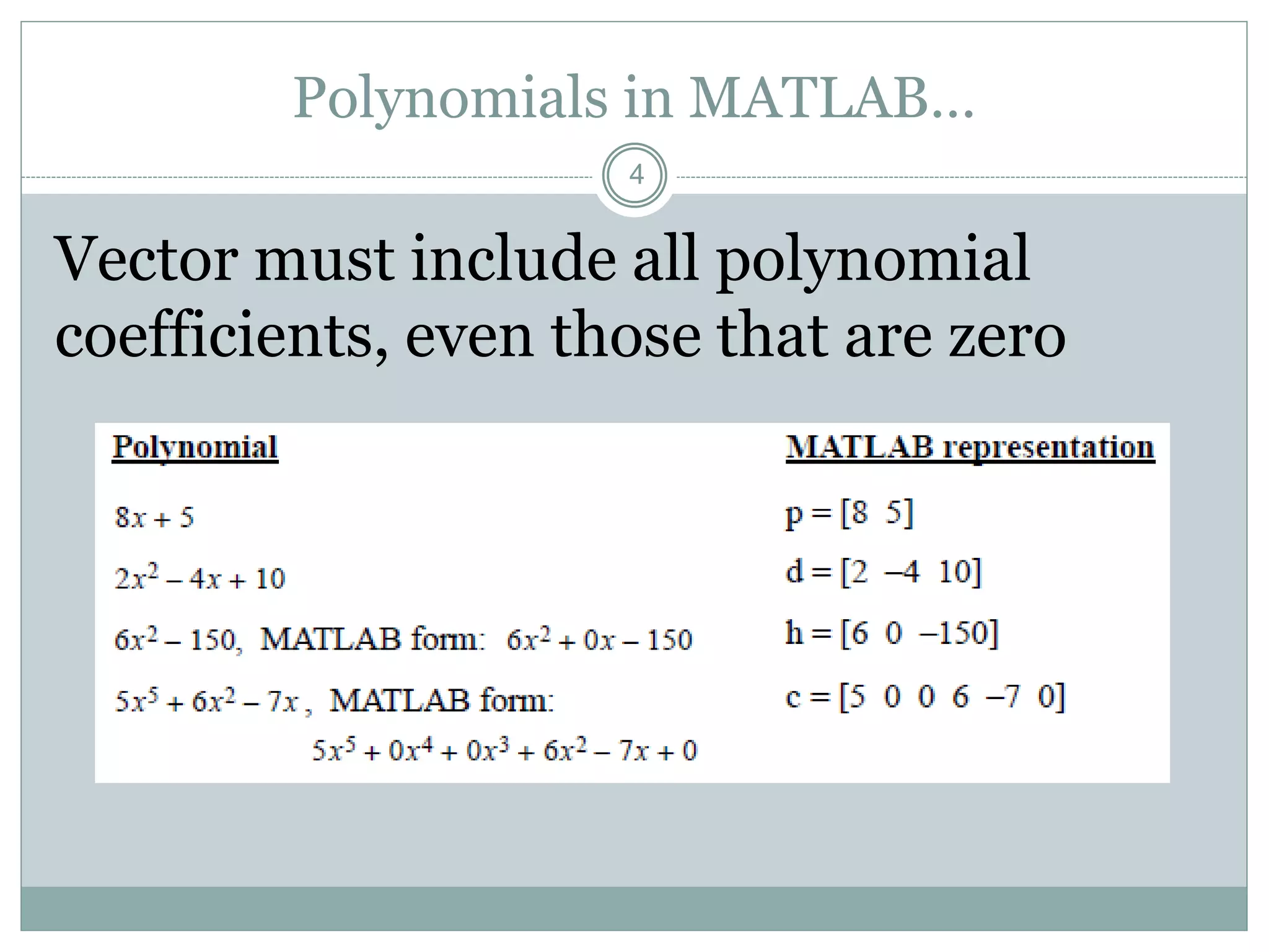
Polynomials are defined in MATLAB as row vectors made up of the
coefficients of the polynomial, whose dimension is n+1, n being the degree
of the polynomial
p = [1 -12 0 25 116] represents x4 - 12x3 + 25x + 116
poly2sym(p)
sym2poly(x^4-12*x^3+25*x+116)
3](https://image.slidesharecdn.com/lecture07polynimialsandcurvefitting-160823082536/75/Polynomials-and-Curve-Fitting-in-MATLAB-3-2048.jpg)
![Value of a Polynomial
MATLAB provides the function polyval to evaluate
polynomials. To use polyval you need to provide the
polynomial to evaluate and the range of values where the
polynomial is to be evaluated. Consider,
>>p = [1 4 -7 -10];
To evaluate p at x=5, use
>> polyval(p,5)
To evaluate for a set of values,
>>x = linspace(-1, 3, 100);
>>y = polyval(p,x);
>>plot(x,y)
>>title(‘Plot of x^3 + 4*x^2 – 7*x – 10’)
>>xlabel(‘x’)
5](https://image.slidesharecdn.com/lecture07polynimialsandcurvefitting-160823082536/75/Polynomials-and-Curve-Fitting-in-MATLAB-5-2048.jpg)
![Roots
>>p = [1, -12, 0, 25, 116]; % 4th order polynomial
(x-r1)(x-r2)(x-r3)(x-r4)
>>r = roots(p)
r =
11.7473
2.7028
-1.2251 + 1.4672i
-1.2251 - 1.4672i
From a set of roots we can also determine the polynomial
>>pp = poly(r)
r =
1 -12 -1.7764e-014 25 116
6](https://image.slidesharecdn.com/lecture07polynimialsandcurvefitting-160823082536/75/Polynomials-and-Curve-Fitting-in-MATLAB-6-2048.jpg)
![Addition and Subtraction
MATLAB does not provide a direct function for adding or subtracting
polynomials unless they are of the same order, when they are of the
same order, normal matrix addition and subtraction applies, d = a + b
and e = a – b are defined when a and b are of the same order.
When they are not of the same order, the lesser order polynomial must
be padded with leading zeroes before adding or subtracting the two
polynomials.
>>p1=[3 15 0 -10 -3 15 -40];
>>p2 = [3 0 -2 -6];
>>p = p1 + [0 0 0 p2];
>>p =
3 15 0 -7 -3 13 -46
The lesser polynomial is padded and then added or subtracted as
appropriate.
7](https://image.slidesharecdn.com/lecture07polynimialsandcurvefitting-160823082536/75/Polynomials-and-Curve-Fitting-in-MATLAB-7-2048.jpg)
![Multiplication
Polynomial multiplication is supported by the conv function. For the
two polynomials
a(x) = x3 + 2x2 + 3x + 4
b(x) = x3 + 4x2 + 9x + 16
>>a = [1 2 3 4];
>>b = [1 4 9 16];
>>c = conv(a,b)
c =
1 6 20 50 75 84 64
or c(x) = x6 + 6x5 + 20x4 + 50x3 + 75x2 + 84x + 64
8](https://image.slidesharecdn.com/lecture07polynimialsandcurvefitting-160823082536/75/Polynomials-and-Curve-Fitting-in-MATLAB-8-2048.jpg)
![Division
Division takes care of the case where we want to divide one polynomial
by another, in MATLAB we use the deconv function. In general
polynomial division yields a quotient polynomial and a remainder
polynomial. Let’s look at two cases;
Case 1: suppose f(x)/g(x) has no remainder;
>>f=[2 9 7 -6];
>>g=[1 3];
>>[q,r] = deconv(f,g)
q =
2 3 -2 q(x) = 2x2 + 3x -2
r =
0 0 0 0 r(x) = 0
10](https://image.slidesharecdn.com/lecture07polynimialsandcurvefitting-160823082536/75/Polynomials-and-Curve-Fitting-in-MATLAB-10-2048.jpg)
![Division II
The representation of r looks strange, but MATLAB outputs
r padding it with leading zeros so that length(r) = length of
f, or length(f).
Case 2: now suppose f(x)/g(x) has a remainder,
>>f=[2 -13 0 75 2 0 -60];
>>g=[1 0 -5];
>>[q,r] = deconv(f,g)
q =
2 -13 10 10 52 q(x) = 2x4 - 13x3 + 10x2 + 10x + 52
r =
0 0 0 0 0 50 200 r(x) = -2x2 – 6x -12
11](https://image.slidesharecdn.com/lecture07polynimialsandcurvefitting-160823082536/75/Polynomials-and-Curve-Fitting-in-MATLAB-11-2048.jpg)
![Derivatives
Single polynomial
k = polyder(p)
Product of polynomials
k = polyder(a,b)
Quotient of two polynomials
[n d] = polyder(u,v)
12](https://image.slidesharecdn.com/lecture07polynimialsandcurvefitting-160823082536/75/Polynomials-and-Curve-Fitting-in-MATLAB-12-2048.jpg)

![Curve Fitting ....
Consider 11 measurements of Voltage for Field current change from 0
to 1 A, spaced 0.1 A.
>>x = [0 .1 .2 .3 .4 .5 .6 .7 .8 .9 1];
>>y = [-.447 1.978 3.28 6.16 7.08 7.34 7.66 9.56 9.48 9.30 11.2];
>>n = 2;
>>p = polyfit( x, y, n )
p =
-9.8108 20.1293 -0.317
or p(x) = -9.8108x2 + 20.1293 – 0.317
>>xi = linspace(0,1,100);
>>yi = polyval(p, xi);
>>plot(x,y,’-o’, xi, yi, ‘-’)
>>xlabel(‘x’), ylabel(‘y = f(x)’)
>>title(‘Second Order Curve Fitting Example’)
15](https://image.slidesharecdn.com/lecture07polynimialsandcurvefitting-160823082536/75/Polynomials-and-Curve-Fitting-in-MATLAB-15-2048.jpg)
![Curve Fitting – 2nd Order Polynomial
Consider the ‘cosine’ function
x = [0:10]; y = [1 0.54 -0.42 -0.99 -0.65 0.28 0.96 0.75 -0.15 -0.91 -0.83];
Start with polynomial of degree 2 (i.e. quadratic):
p=polyfit(x,y,2)
p =
-0.0040 -0.0427 0.3152
So the polynomial is
-0.0040x2 - 0.0427x + 0.3152
17](https://image.slidesharecdn.com/lecture07polynimialsandcurvefitting-160823082536/75/Polynomials-and-Curve-Fitting-in-MATLAB-17-2048.jpg)


![Polynomials in MATLAB
MATLAB provides a number of functions for the
manipulation of polynomials. These include,
Evaluation of polynomials
Finding roots of polynomials
Addition, subtraction, multiplication, and division of polynomials
Dealing with rational expressions of polynomials
Curve fitting
Polynomials are defined in MATLAB as row vectors made up of the
coefficients of the polynomial, whose dimension is n+1, n being the degree
of the polynomial
p = [1 -12 0 25 116] represents x4 - 12x3 + 25x + 116
poly2sym(p)
sym2poly(x^4-12*x^3+25*x+116)
3](https://crownmelresort.com/image.slidesharecdn.com/lecture07polynimialsandcurvefitting-160823082536/75/Polynomials-and-Curve-Fitting-in-MATLAB-3-2048.jpg)

![Value of a Polynomial
MATLAB provides the function polyval to evaluate
polynomials. To use polyval you need to provide the
polynomial to evaluate and the range of values where the
polynomial is to be evaluated. Consider,
>>p = [1 4 -7 -10];
To evaluate p at x=5, use
>> polyval(p,5)
To evaluate for a set of values,
>>x = linspace(-1, 3, 100);
>>y = polyval(p,x);
>>plot(x,y)
>>title(‘Plot of x^3 + 4*x^2 – 7*x – 10’)
>>xlabel(‘x’)
5](https://crownmelresort.com/image.slidesharecdn.com/lecture07polynimialsandcurvefitting-160823082536/75/Polynomials-and-Curve-Fitting-in-MATLAB-5-2048.jpg)
![Roots
>>p = [1, -12, 0, 25, 116]; % 4th order polynomial
(x-r1)(x-r2)(x-r3)(x-r4)
>>r = roots(p)
r =
11.7473
2.7028
-1.2251 + 1.4672i
-1.2251 - 1.4672i
From a set of roots we can also determine the polynomial
>>pp = poly(r)
r =
1 -12 -1.7764e-014 25 116
6](https://crownmelresort.com/image.slidesharecdn.com/lecture07polynimialsandcurvefitting-160823082536/75/Polynomials-and-Curve-Fitting-in-MATLAB-6-2048.jpg)
![Addition and Subtraction
MATLAB does not provide a direct function for adding or subtracting
polynomials unless they are of the same order, when they are of the
same order, normal matrix addition and subtraction applies, d = a + b
and e = a – b are defined when a and b are of the same order.
When they are not of the same order, the lesser order polynomial must
be padded with leading zeroes before adding or subtracting the two
polynomials.
>>p1=[3 15 0 -10 -3 15 -40];
>>p2 = [3 0 -2 -6];
>>p = p1 + [0 0 0 p2];
>>p =
3 15 0 -7 -3 13 -46
The lesser polynomial is padded and then added or subtracted as
appropriate.
7](https://crownmelresort.com/image.slidesharecdn.com/lecture07polynimialsandcurvefitting-160823082536/75/Polynomials-and-Curve-Fitting-in-MATLAB-7-2048.jpg)
![Multiplication
Polynomial multiplication is supported by the conv function. For the
two polynomials
a(x) = x3 + 2x2 + 3x + 4
b(x) = x3 + 4x2 + 9x + 16
>>a = [1 2 3 4];
>>b = [1 4 9 16];
>>c = conv(a,b)
c =
1 6 20 50 75 84 64
or c(x) = x6 + 6x5 + 20x4 + 50x3 + 75x2 + 84x + 64
8](https://crownmelresort.com/image.slidesharecdn.com/lecture07polynimialsandcurvefitting-160823082536/75/Polynomials-and-Curve-Fitting-in-MATLAB-8-2048.jpg)

![Division
Division takes care of the case where we want to divide one polynomial
by another, in MATLAB we use the deconv function. In general
polynomial division yields a quotient polynomial and a remainder
polynomial. Let’s look at two cases;
Case 1: suppose f(x)/g(x) has no remainder;
>>f=[2 9 7 -6];
>>g=[1 3];
>>[q,r] = deconv(f,g)
q =
2 3 -2 q(x) = 2x2 + 3x -2
r =
0 0 0 0 r(x) = 0
10](https://crownmelresort.com/image.slidesharecdn.com/lecture07polynimialsandcurvefitting-160823082536/75/Polynomials-and-Curve-Fitting-in-MATLAB-10-2048.jpg)
![Division II
The representation of r looks strange, but MATLAB outputs
r padding it with leading zeros so that length(r) = length of
f, or length(f).
Case 2: now suppose f(x)/g(x) has a remainder,
>>f=[2 -13 0 75 2 0 -60];
>>g=[1 0 -5];
>>[q,r] = deconv(f,g)
q =
2 -13 10 10 52 q(x) = 2x4 - 13x3 + 10x2 + 10x + 52
r =
0 0 0 0 0 50 200 r(x) = -2x2 – 6x -12
11](https://crownmelresort.com/image.slidesharecdn.com/lecture07polynimialsandcurvefitting-160823082536/75/Polynomials-and-Curve-Fitting-in-MATLAB-11-2048.jpg)
![Derivatives
Single polynomial
k = polyder(p)
Product of polynomials
k = polyder(a,b)
Quotient of two polynomials
[n d] = polyder(u,v)
12](https://crownmelresort.com/image.slidesharecdn.com/lecture07polynimialsandcurvefitting-160823082536/75/Polynomials-and-Curve-Fitting-in-MATLAB-12-2048.jpg)


![Curve Fitting ....
Consider 11 measurements of Voltage for Field current change from 0
to 1 A, spaced 0.1 A.
>>x = [0 .1 .2 .3 .4 .5 .6 .7 .8 .9 1];
>>y = [-.447 1.978 3.28 6.16 7.08 7.34 7.66 9.56 9.48 9.30 11.2];
>>n = 2;
>>p = polyfit( x, y, n )
p =
-9.8108 20.1293 -0.317
or p(x) = -9.8108x2 + 20.1293 – 0.317
>>xi = linspace(0,1,100);
>>yi = polyval(p, xi);
>>plot(x,y,’-o’, xi, yi, ‘-’)
>>xlabel(‘x’), ylabel(‘y = f(x)’)
>>title(‘Second Order Curve Fitting Example’)
15](https://crownmelresort.com/image.slidesharecdn.com/lecture07polynimialsandcurvefitting-160823082536/75/Polynomials-and-Curve-Fitting-in-MATLAB-15-2048.jpg)

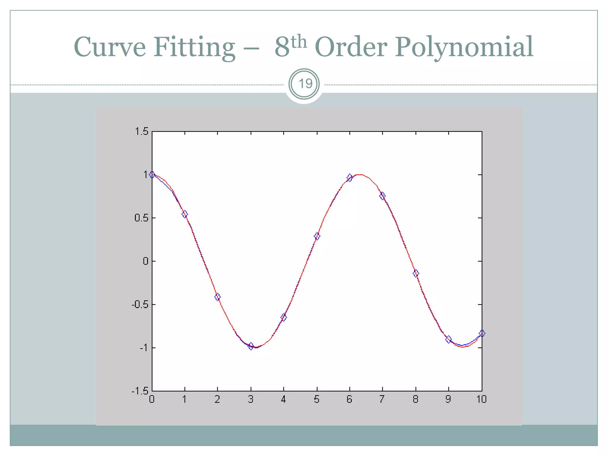
![Curve Fitting – 2nd Order Polynomial
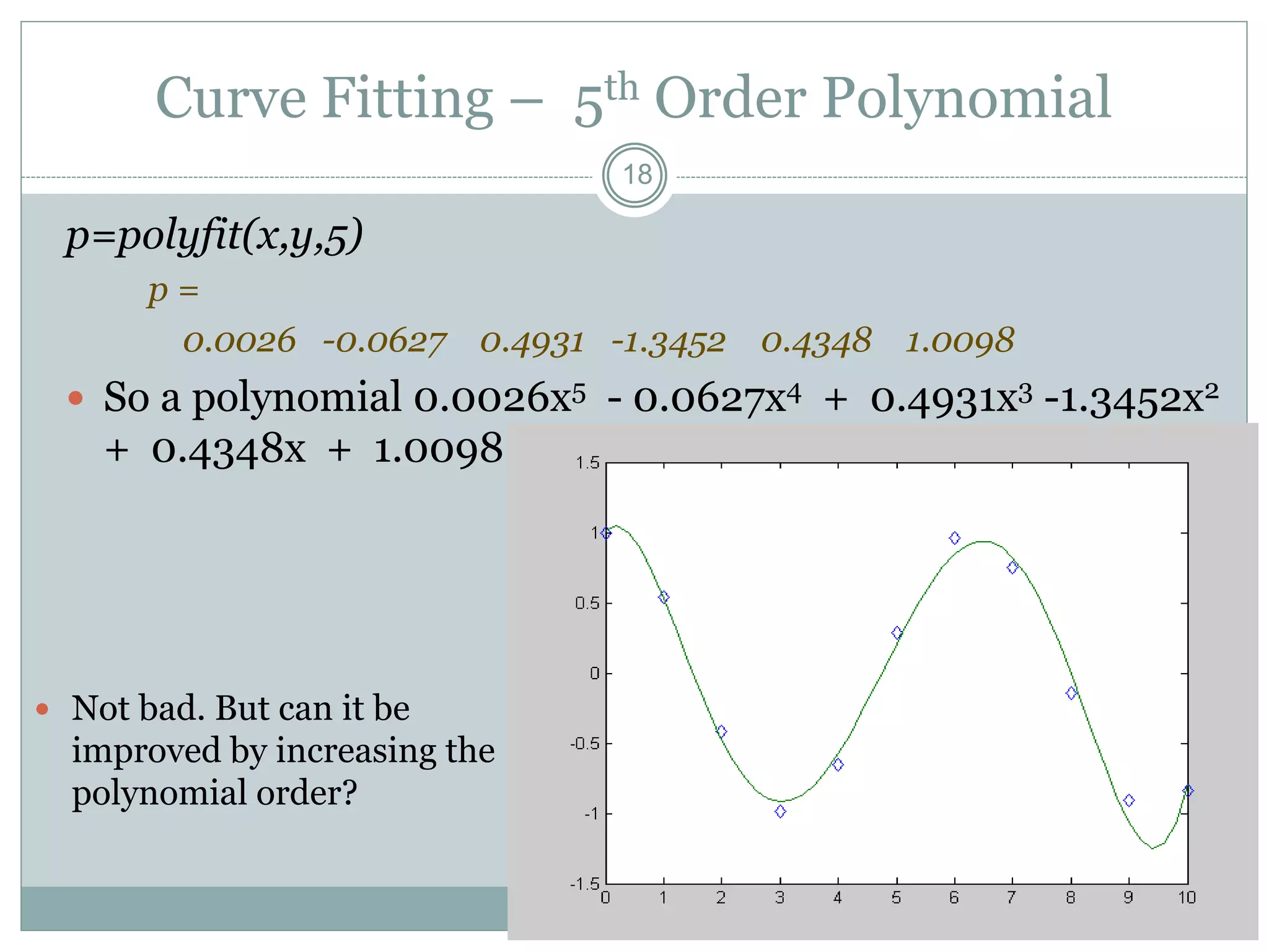
Consider the ‘cosine’ function
x = [0:10]; y = [1 0.54 -0.42 -0.99 -0.65 0.28 0.96 0.75 -0.15 -0.91 -0.83];
Start with polynomial of degree 2 (i.e. quadratic):
p=polyfit(x,y,2)
p =
-0.0040 -0.0427 0.3152
So the polynomial is
-0.0040x2 - 0.0427x + 0.3152
17](https://crownmelresort.com/image.slidesharecdn.com/lecture07polynimialsandcurvefitting-160823082536/75/Polynomials-and-Curve-Fitting-in-MATLAB-17-2048.jpg)


This document discusses various polynomial functions in MATLAB. It covers defining and manipulating polynomials, including evaluation, finding roots, addition/subtraction, multiplication/division, derivatives, and curve fitting using polynomial regression. Polynomials in MATLAB are defined as row vectors of coefficients. Key functions include polyval for evaluation, roots for finding roots, conv for multiplication, deconv for division, and polyfit for curve fitting.