matlab pde toolbox

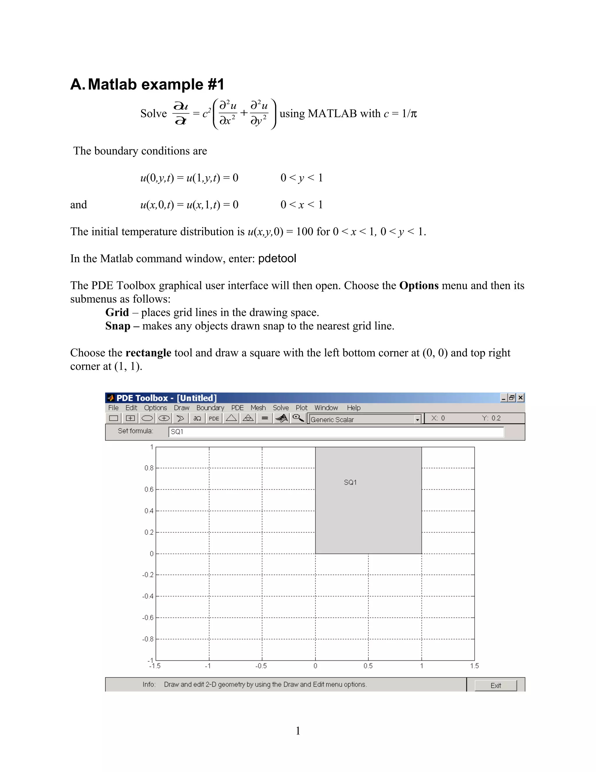
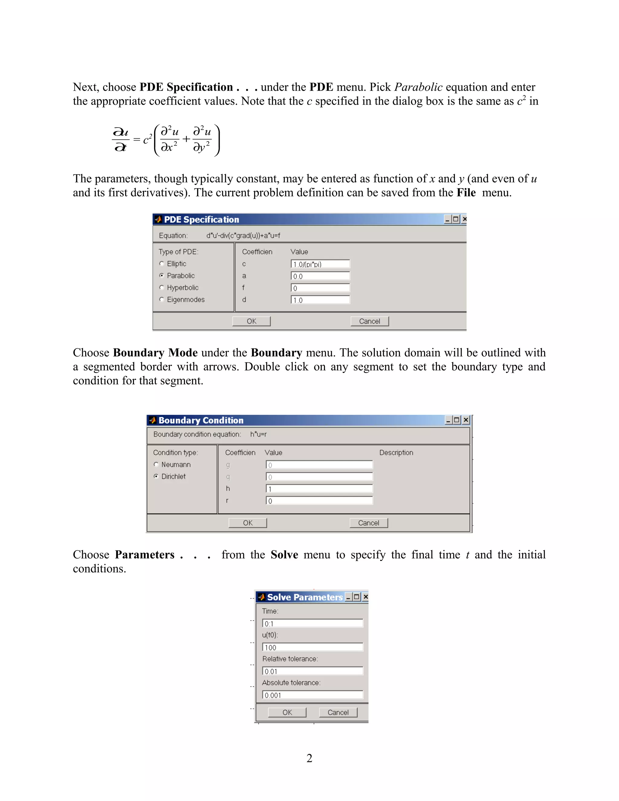
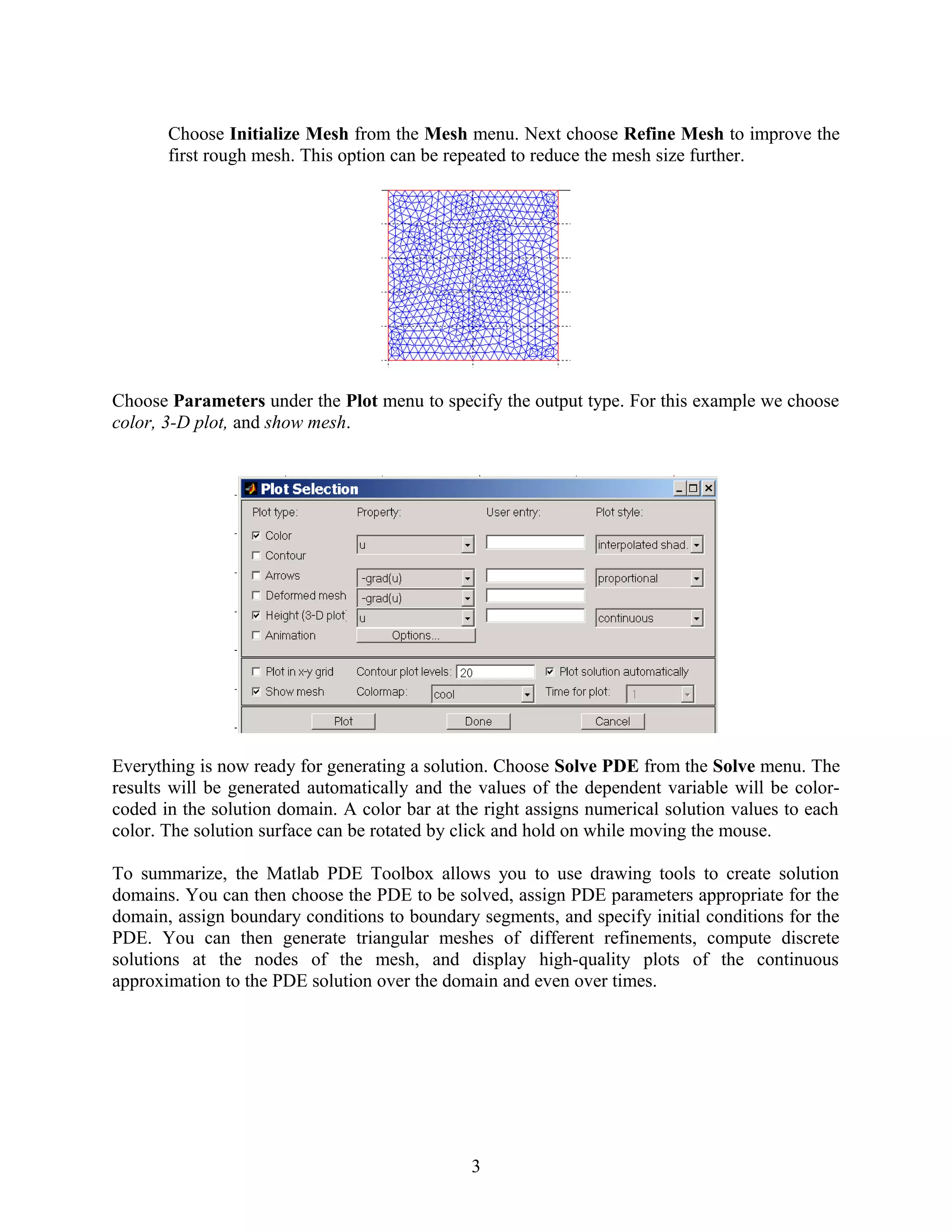
A.Matlab example #1
Solve
t
u
∂
∂
= c2






∂
∂
+
∂
∂
2
2
2
2
y
u
x
u
using MATLAB with c = 1/π
The boundary conditions are
u(0,y,t) = u(1,y,t) = 0 0 < y < 1
and u(x,0,t) = u(x,1,t) = 0 0 < x < 1
The initial temperature distribution is u(x,y,0) = 100 for 0 < x < 1, 0 < y < 1.
In the Matlab command window, enter: pdetool
The PDE Toolbox graphical user interface will then open. Choose the Options menu and then its
submenus as follows:
Grid – places grid lines in the drawing space.
Snap – makes any objects drawn snap to the nearest grid line.
Choose the rectangle tool and draw a square with the left bottom corner at (0, 0) and top right
corner at (1, 1).
1

Next, choose PDE Specification . . . under the PDE menu. Pick Parabolic equation and enter
the appropriate coefficient values. Note that the c specified in the dialog box is the same as c2
in
t
u
∂
∂
= c2






∂
∂
+
∂
∂
2
2
2
2
y
u
x
u
The parameters, though typically constant, may be entered as function of x and y (and even of u
and its first derivatives). The current problem definition can be saved from the File menu.
Choose Boundary Mode under the Boundary menu. The solution domain will be outlined with
a segmented border with arrows. Double click on any segment to set the boundary type and
condition for that segment.
Choose Parameters . . . from the Solve menu to specify the final time t and the initial
conditions.
2

Choose Initialize Mesh from the Mesh menu. Next choose Refine Mesh to improve the
first rough mesh. This option can be repeated to reduce the mesh size further.
Choose Parameters under the Plot menu to specify the output type. For this example we choose
color, 3-D plot, and show mesh.
Everything is now ready for generating a solution. Choose Solve PDE from the Solve menu. The
results will be generated automatically and the values of the dependent variable will be color-
coded in the solution domain. A color bar at the right assigns numerical solution values to each
color. The solution surface can be rotated by click and hold on while moving the mouse.
To summarize, the Matlab PDE Toolbox allows you to use drawing tools to create solution
domains. You can then choose the PDE to be solved, assign PDE parameters appropriate for the
domain, assign boundary conditions to boundary segments, and specify initial conditions for the
PDE. You can then generate triangular meshes of different refinements, compute discrete
solutions at the nodes of the mesh, and display high-quality plots of the continuous
approximation to the PDE solution over the domain and even over times.
3

2
4
6
8
10
12
14
16
18
20
0
0.2
0.4
0.6
0.8
1
0
0.2
0.4
0.6
0.8
1
0
5
10
15
20
25
Time=1 Color: u Height: u
The composite drawing is taken to be the union of all drawn objects in the set sense. If you want
the domain to be a rectangle with an ellipse hole in it, just edit the Set formula: field to contain
R1 − E1.
4

matlab pde toolbox

More Related Content

What's hot

Similar to matlab pde toolbox

Recently uploaded

matlab pde toolbox