Introduction to MATLAB

Introduction to MATLAB
and Simulink
Presented by:
Ravikiran B. A.
Asst. Professor, Dept of ECE
KSSEM

What is MATLAB®?
• “The Language of Technical Computing”
• Numerical Programming Environment
• MATLAB - MATrix LABoratory
• High-Level Interpreted Language
• Uses:
• Analyze Data
• Develop Algorithms
• Create Models and Applications.
• Multidisciplinary Applications
2
Introduction to MATLAB and Simulink
K. S. School of Engineering and Management

• Acquire and Analyze Data from different sources
• Data from Measuring and Sensing Instruments
• Recorded Data (Spreadsheets, text files, images, audio files, etc)
• Analyze Data using different tools
• Develop Functions and Algorithms
• Visualize Data in terms of graphs, plots, etc
• Simulink is used to Develop Models and Applications
• Deploy Code as Standalone Applications
K. S. School of Engineering and Management 3
What Can I Do with MATLAB?

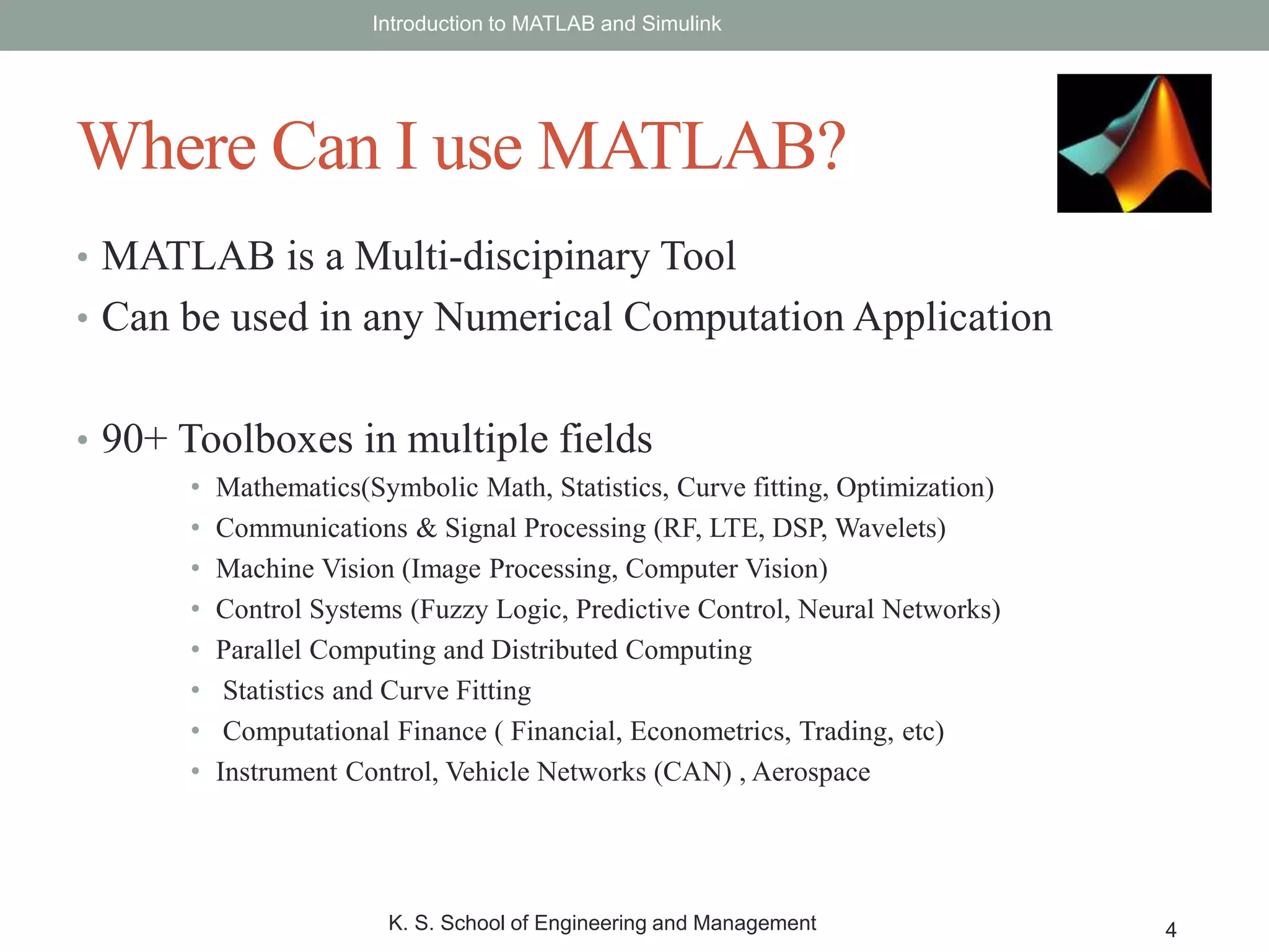
• MATLAB is a Multi-discipinary Tool
• Can be used in any Numerical Computation Application
• 90+ Toolboxes in multiple fields
• Mathematics(Symbolic Math, Statistics, Curve fitting, Optimization)
• Communications & Signal Processing (RF, LTE, DSP, Wavelets)
• Machine Vision (Image Processing, Computer Vision)
• Control Systems (Fuzzy Logic, Predictive Control, Neural Networks)
• Parallel Computing and Distributed Computing
• Statistics and Curve Fitting
• Computational Finance ( Financial, Econometrics, Trading, etc)
• Instrument Control, Vehicle Networks (CAN) , Aerospace
Where Can I use MATLAB?

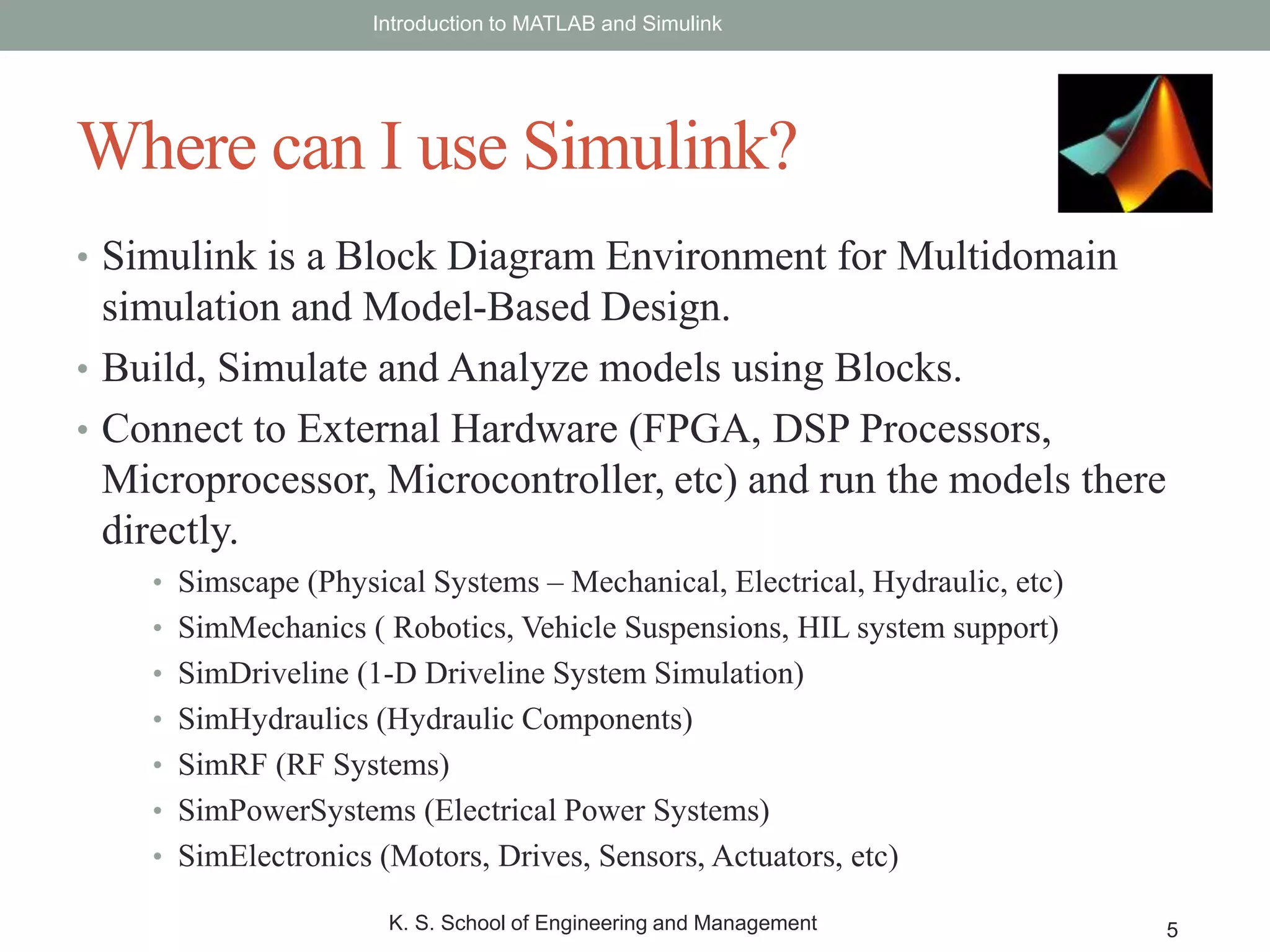
• Simulink is a Block Diagram Environment for Multidomain
simulation and Model-Based Design.
• Build, Simulate and Analyze models using Blocks.
• Connect to External Hardware (FPGA, DSP Processors,
Microprocessor, Microcontroller, etc) and run the models there
directly.
• Simscape (Physical Systems – Mechanical, Electrical, Hydraulic, etc)
• SimMechanics ( Robotics, Vehicle Suspensions, HIL system support)
• SimDriveline (1-D Driveline System Simulation)
• SimHydraulics (Hydraulic Components)
• SimRF (RF Systems)
• SimPowerSystems (Electrical Power Systems)
• SimElectronics (Motors, Drives, Sensors, Actuators, etc)
Where can I use Simulink?

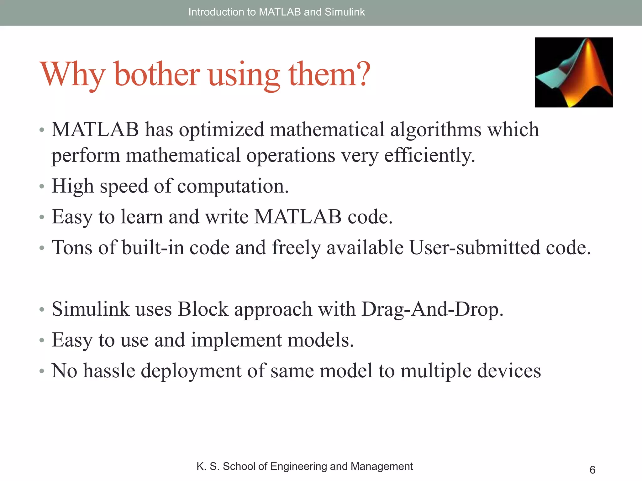
• MATLAB has optimized mathematical algorithms which
perform mathematical operations very efficiently.
• High speed of computation.
• Easy to learn and write MATLAB code.
• Tons of built-in code and freely available User-submitted code.
• Simulink uses Block approach with Drag-And-Drop.
• Easy to use and implement models.
• No hassle deployment of same model to multiple devices
Why bother using them?

The MATLAB Screen
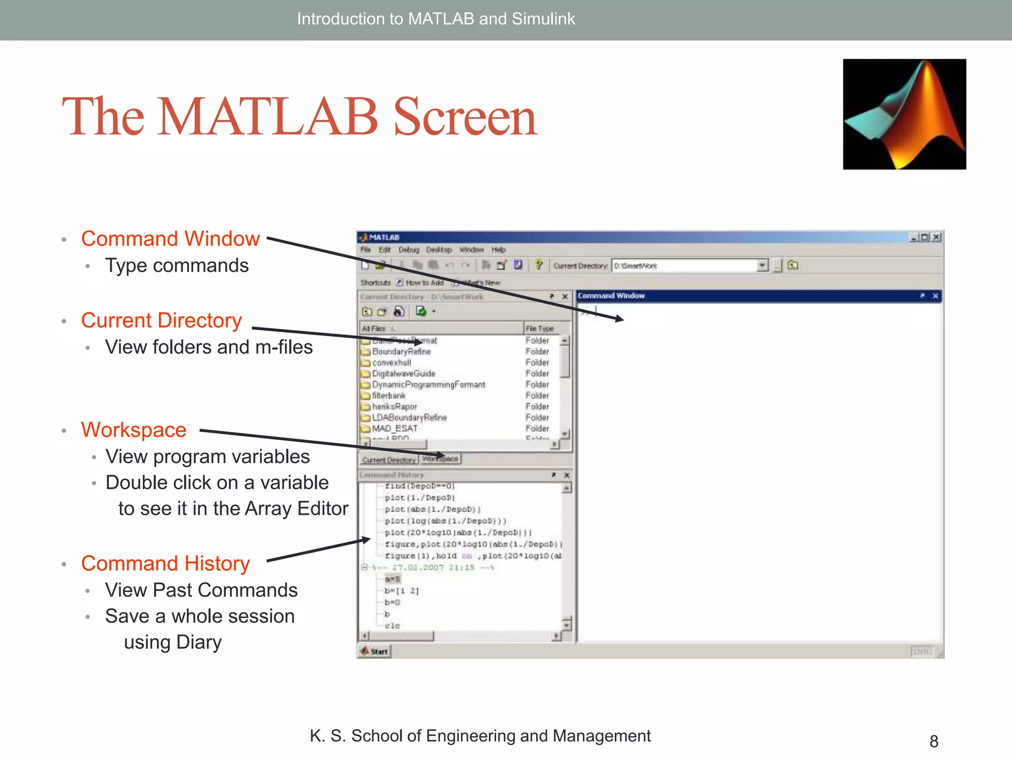
• Command Window
• Type commands
• Current Directory
• View folders and m-files
• Workspace
• View program variables
• Double click on a variable
to see it in the Array Editor
• Command History
• View Past Commands
• Save a whole session
using Diary

• MATLAB works primarily (almost exclusively) with matrices.
• MATLAB functions are optimized to handle matrix operations.
• MATLAB can handle upto 13-dimensional matrices.
• Loops can be vectorized for faster operations.
Matrices – Matrices Everywhere

• Matrix is a one- or multi-dimensional array of elements.
• Elements can be numerical, variables or string elements.
• By default, MATLAB stores numbers as double precision.
• ALL data in MATLAB are viewed as matrices.
• Matrices can be:
• Created Manually by User
• Generated by MATLAB Functions
• Imported from stored databases or files
Matrices -Arrays and Vectors

• Unlike C, MATLAB is an interpreted language. So, there is no
need for Type Declaration.
• A single variable is interpreted as 1x1 matrix.
>> a = 5
a =
5
• Arrays are represented as a series of numbers (or characters)
within square brackets, with or without a comma separating the
values.
>> b = [1 2 3 4 5] % Percentage Symbol indicates Comment
b =
1 2 3 4 5
Array Declaration

• 2-D or Multidimensional Arrays are represented within square
brackets, with the ; (semicolon) operator indicating end of a
row.
>> c = [1 2 3 ; 4 5 6 ; 7 8 9 ; 10 11 12]
c =
1 2 3
4 5 6
7 8 9
10 11 12
• c is now a 2-D array with 4 rows and 3 columns
Note : Variable names are case sensitive and can be upto 31 characters long, and have
to start with an alphabet.
MultidimensionalArrays

• Character strings are treated as arrays too.
>> name = 'Ravi’
is the same as
>> name = [‘R’ ‘a’ ‘v’ ‘i’]
And gives the output:
name =
Ravi
• Strings and Characters are both declared within SINGLE
quotes (‘ ’)
Strings

• Unlike in case of C, MATLAB array indices start from 1.
>> d = [1 2 3 ; 4 5 6]
d =
1 2 3
4 5 6
• Addressing an element of the array is done by invoking the
element’s row and column number.
• In order to fetch the value of an element in the 2nd row and 3rd
column, we use:
>> e = d(2,3)
e =
6
Array Indices

• Rather than addressing single elements, we can also use
commands to address multiple elements in an array.
• The ‘:’ (colon) operator is used to address all elements in a row
or column.
• The ‘:’ operator basically tells the interpreter to address ALL
elements.
• The ‘:’ operator can also be used to indicate a range of indices.
Addressing multiple elements

• Consider the earlier example: d = [1 2 3; 4 5 6]
• >> f = d(1, :) % Address All elements of 1st Row
f =
1 2 3
• >> g = d(:,2) % Address All elements in 2nd Column
g =
2
5
>> h = d(1:2,1:2) %Address Rows from 1 to 2 and Columns from 1 to 2
h =
1 2
4 5

• In some cases, we need to generate large matrices, which is difficult
to generate manually.
• There are plenty of built-in commands for this purpose!
• >> i = 0:10 % Generate numbers from 0 to 10 (Integers)
i =
0 1 2 3 4 5 6 7 8 9 10
• >> j = 0:0.2:1 % Generate numbers from 0 to 1, in steps of 0.2
j =
0 0.2000 0.4000 0.6000 0.8000 1.0000
• >> k = [1:3; 4:6;7:9] % Generate a 3x3 matrix of numbers 1 through 9
k =
1 2 3
4 5 6
7 8 9
Generating Matrices

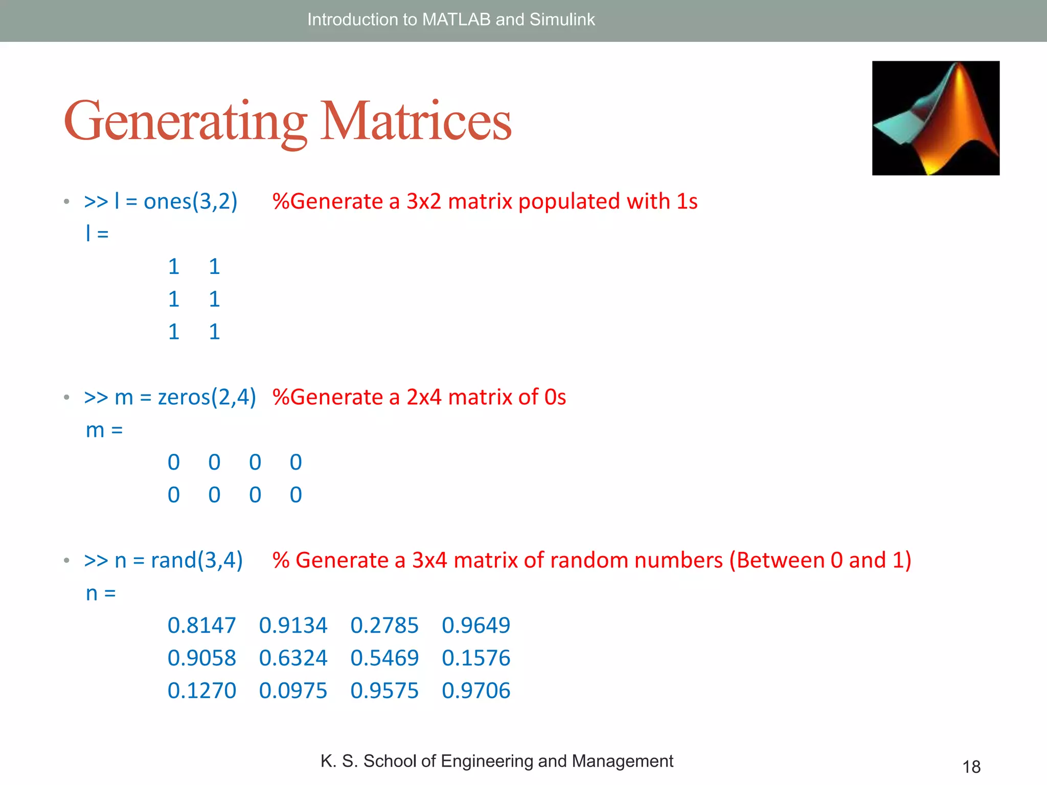
• >> l = ones(3,2) %Generate a 3x2 matrix populated with 1s
l =
1 1
1 1
1 1
• >> m = zeros(2,4) %Generate a 2x4 matrix of 0s
m =
0 0 0 0
0 0 0 0
• >> n = rand(3,4) % Generate a 3x4 matrix of random numbers (Between 0 and 1)
n =
0.8147 0.9134 0.2785 0.9649
0.9058 0.6324 0.5469 0.1576
0.1270 0.0975 0.9575 0.9706
Generating Matrices

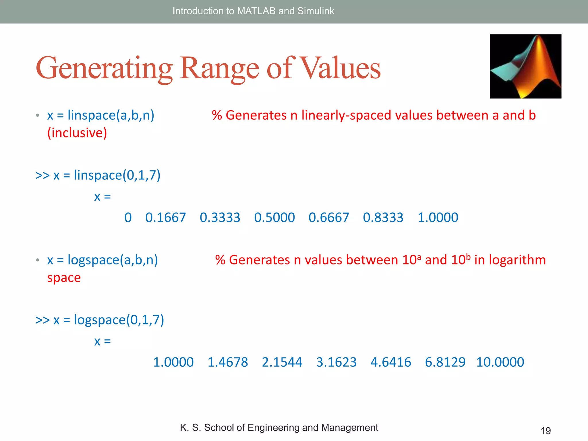
• x = linspace(a,b,n) % Generates n linearly-spaced values between a and b
(inclusive)
>> x = linspace(0,1,7)
x =
0 0.1667 0.3333 0.5000 0.6667 0.8333 1.0000
• x = logspace(a,b,n) % Generates n values between 10a and 10b in logarithm
space
>> x = logspace(0,1,7)
x =
1.0000 1.4678 2.1544 3.1623 4.6416 6.8129 10.0000
Generating Range of Values

• Operations upon Matrices can be of two types:
• Element-wise Operation
• Matrix-wise Operation
• Common Arithmetic Operations:
• Addition (+)
• Subtraction (-)
• Multiplication (*)
• Division (/)
• Exponentiation (^)
• Matrix Inverse (inv)
• Left Division () [AB is equivalent to INV(A)*B]
• Complex Conjugate Transpose (’)
Matrix Operations

• By default, the Operators perform Matrix-wise operations.
• During Matrix-wise operations, care must be taken to avoid
dimension mismatch, specially with exponentiation, division
and multiplication.
• In case of scalar + matrix operations, matrix-wise operations are
equivalent to element-wise operations.
• ie.
Scalar + Matrix = [Scalar + Matrix(i,j)]
Scalar * Matrix = [Scalar * Matrix(i,j)]
• A dot operator(.) preceding the operator indicates Element-wise
operations.
Matrix Operations

• Let a = [2 5; 8 1]; % 2 x 2 Matrix
b = [1 2 3; 4 5 6]; % 2 x 3 Matrix
c = [1 3; 5 2; 4 6]; % 3 x 2 Matrix
• Matrix Addition (or Subtraction):
>> y = b+c' % b and c have different dimensions.
y =
2 5 8
6 9 12
• Complement:
>> d = c' % d is now a 2x3 matrix
d =
1 5 4
3 2 6
Examples

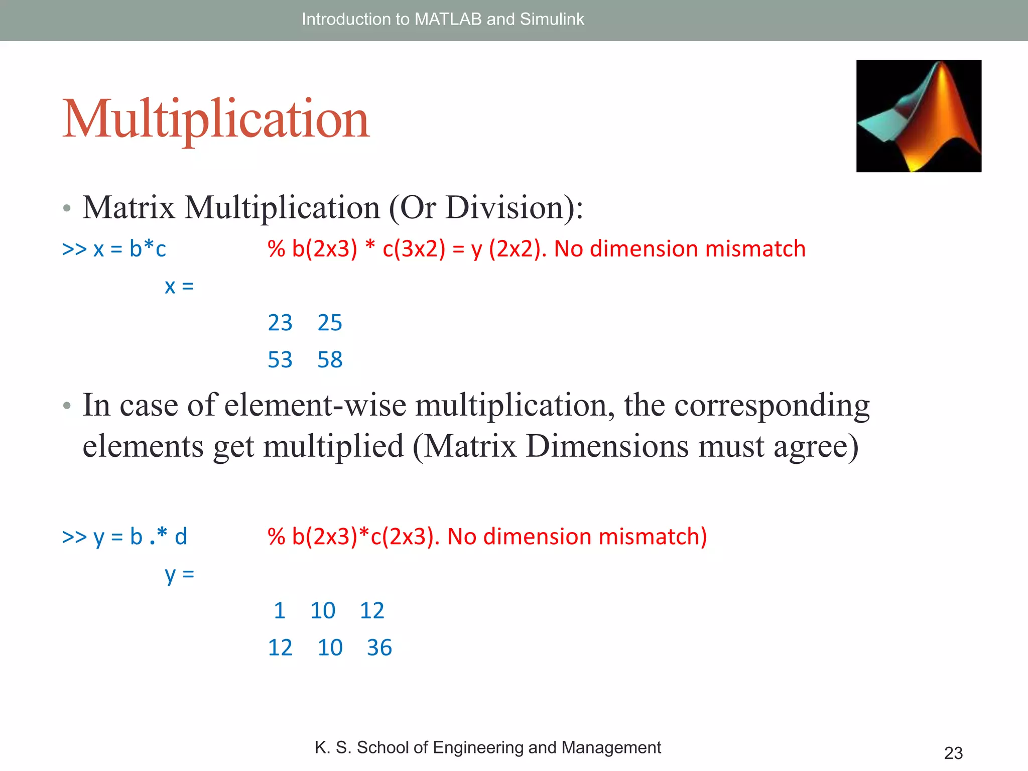
• Matrix Multiplication (Or Division):
>> x = b*c % b(2x3) * c(3x2) = y (2x2). No dimension mismatch
x =
23 25
53 58
• In case of element-wise multiplication, the corresponding
elements get multiplied (Matrix Dimensions must agree)
>> y = b .* d % b(2x3)*c(2x3). No dimension mismatch)
y =
1 10 12
12 10 36
Multiplication

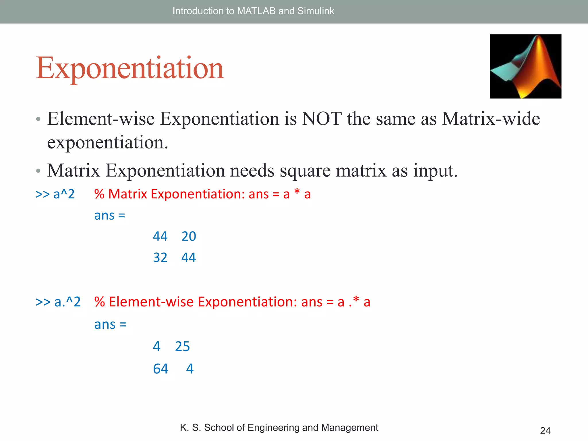
• Element-wise Exponentiation is NOT the same as Matrix-wide
exponentiation.
• Matrix Exponentiation needs square matrix as input.
>> a^2 % Matrix Exponentiation: ans = a * a
ans =
44 20
32 44
>> a.^2 % Element-wise Exponentiation: ans = a .* a
ans =
4 25
64 4
Exponentiation

• Matrices can be concatenated just like elements in a matrix.
• Row-wise concatenation ( separated by space or commas)
>> f = [b d]
f =
1 2 3 1 5 4
4 5 6 3 2 6
• Column-wise concatenation (separated by semicolon)
>> g = [b ; d]
g =
1 2 3
4 5 6
1 5 4
3 2 6
Matrix Concatenation

• >> randn(n) % Generates a (n x n) Normally Distributed Random Matrix
• >> eye(n) % Generates a (n x n) Identity Matrix
• >> magic(n) % Generates a (n x n) Magic Matrix (Same Sum along Row, Column
and Diagonal)
• >> diag(A) % Extracts the elements along the primary diagonal of Matrix A
• >> blockdiag(A,B,C,..) % Generates a block diagonal matrix, with A, B, C, .. As
diagonal elements.
• >> length(x) % Calculates length of a vector x
• >> [m,n] = size(x) % Gives the [Rows,Columns] size of vector x
• >> floor (x) % Round x towards negative infinity (Floor)
• >> ceil (x) % Round x towards positive infinity (Ceiling)
• >> clc % Clears Command Window
• >> clear % Clears the Workspace Variables
• >> close % Close Figure Windows
• >>a = [] %Generates an Empty Matrix
Other useful basic functions

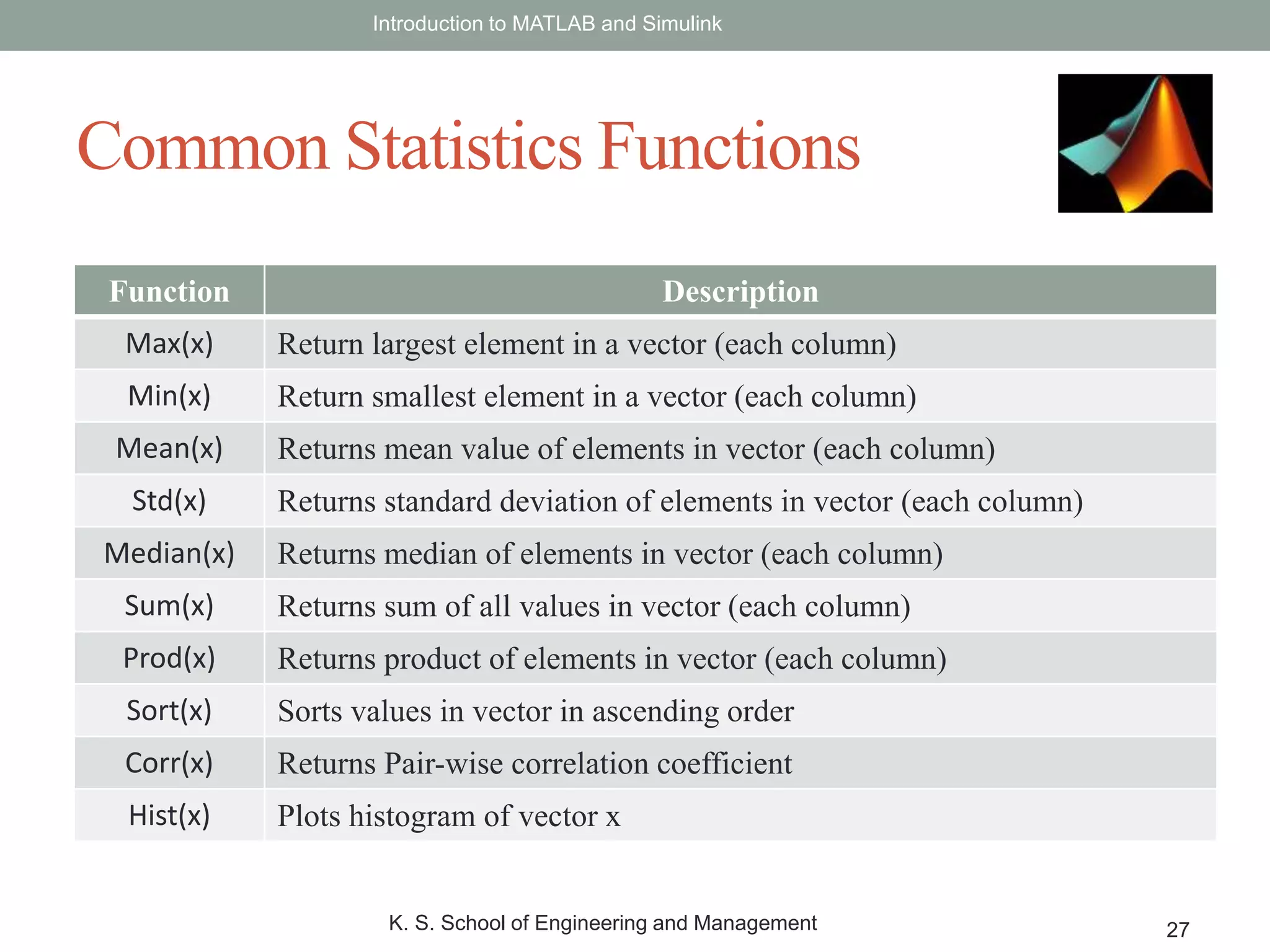
Function Description
Max(x) Return largest element in a vector (each column)
Min(x) Return smallest element in a vector (each column)
Mean(x) Returns mean value of elements in vector (each column)
Std(x) Returns standard deviation of elements in vector (each column)
Median(x) Returns median of elements in vector (each column)
Sum(x) Returns sum of all values in vector (each column)
Prod(x) Returns product of elements in vector (each column)
Sort(x) Sorts values in vector in ascending order
Corr(x) Returns Pair-wise correlation coefficient
Hist(x) Plots histogram of vector x
Common Statistics Functions

VISUALIZATIONS AND
GRAPHICS
Graphs, plots and Histograms

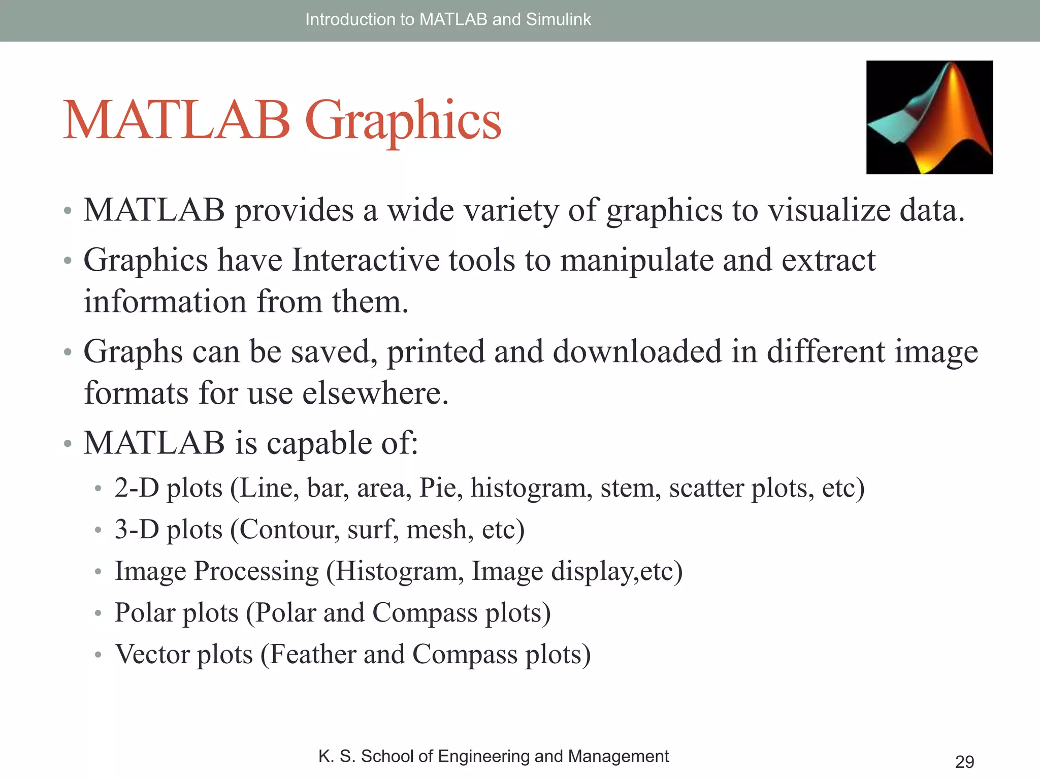
• MATLAB provides a wide variety of graphics to visualize data.
• Graphics have Interactive tools to manipulate and extract
information from them.
• Graphs can be saved, printed and downloaded in different image
formats for use elsewhere.
• MATLAB is capable of:
• 2-D plots (Line, bar, area, Pie, histogram, stem, scatter plots, etc)
• 3-D plots (Contour, surf, mesh, etc)
• Image Processing (Histogram, Image display,etc)
• Polar plots (Polar and Compass plots)
• Vector plots (Feather and Compass plots)
MATLAB Graphics

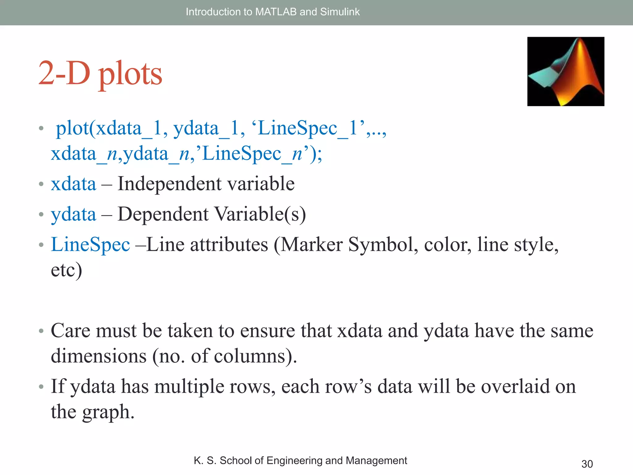
• plot(xdata_1, ydata_1, ‘LineSpec_1’,..,
xdata_n,ydata_n,’LineSpec_n’);
• xdata – Independent variable
• ydata – Dependent Variable(s)
• LineSpec –Line attributes (Marker Symbol, color, line style,
etc)
• Care must be taken to ensure that xdata and ydata have the same
dimensions (no. of columns).
• If ydata has multiple rows, each row’s data will be overlaid on
the graph.
2-D plots

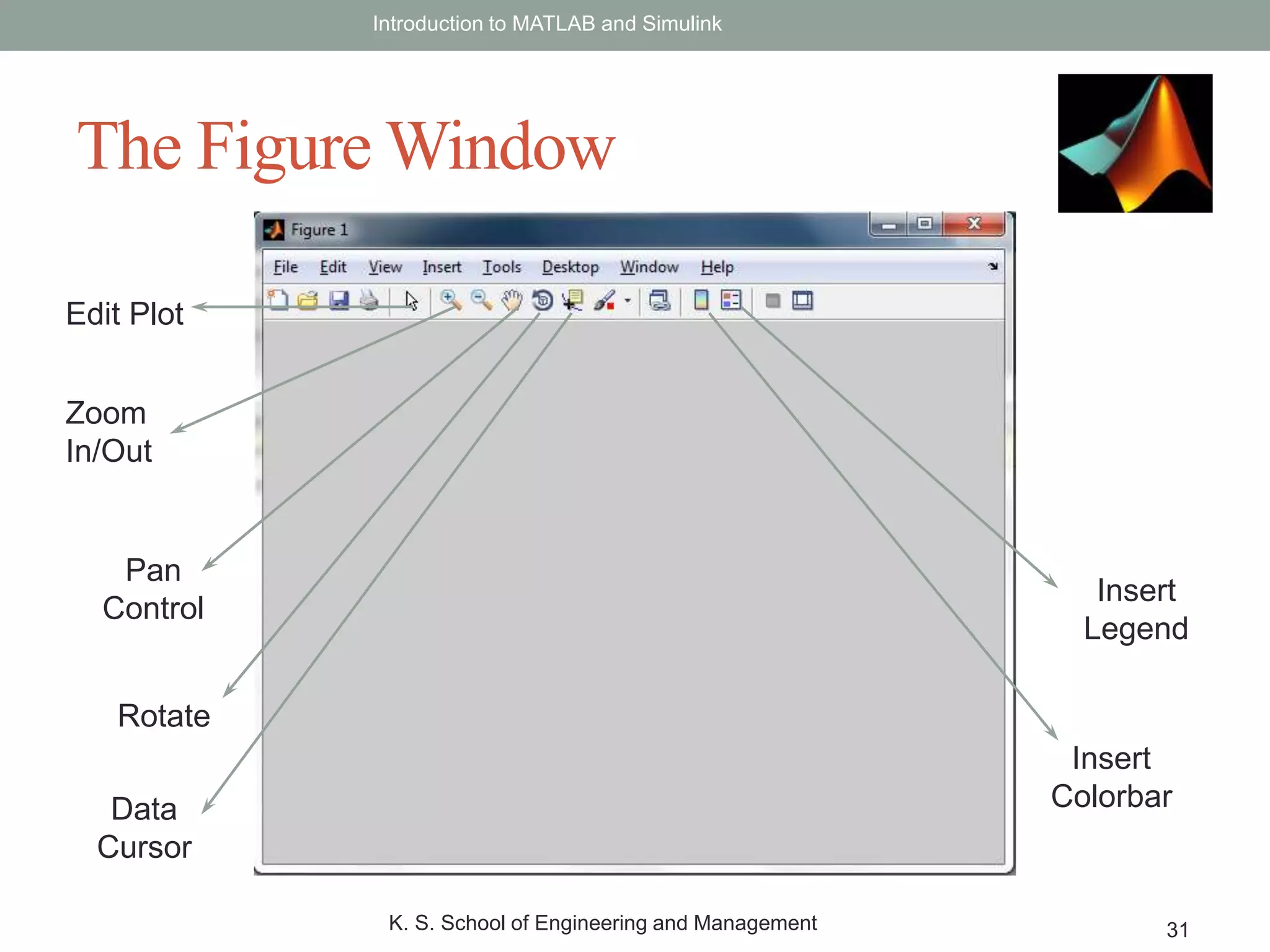
The Figure Window
Edit Plot
Zoom
In/Out
Pan
Control
Rotate
Data
Cursor
Insert
Colorbar
Insert
Legend

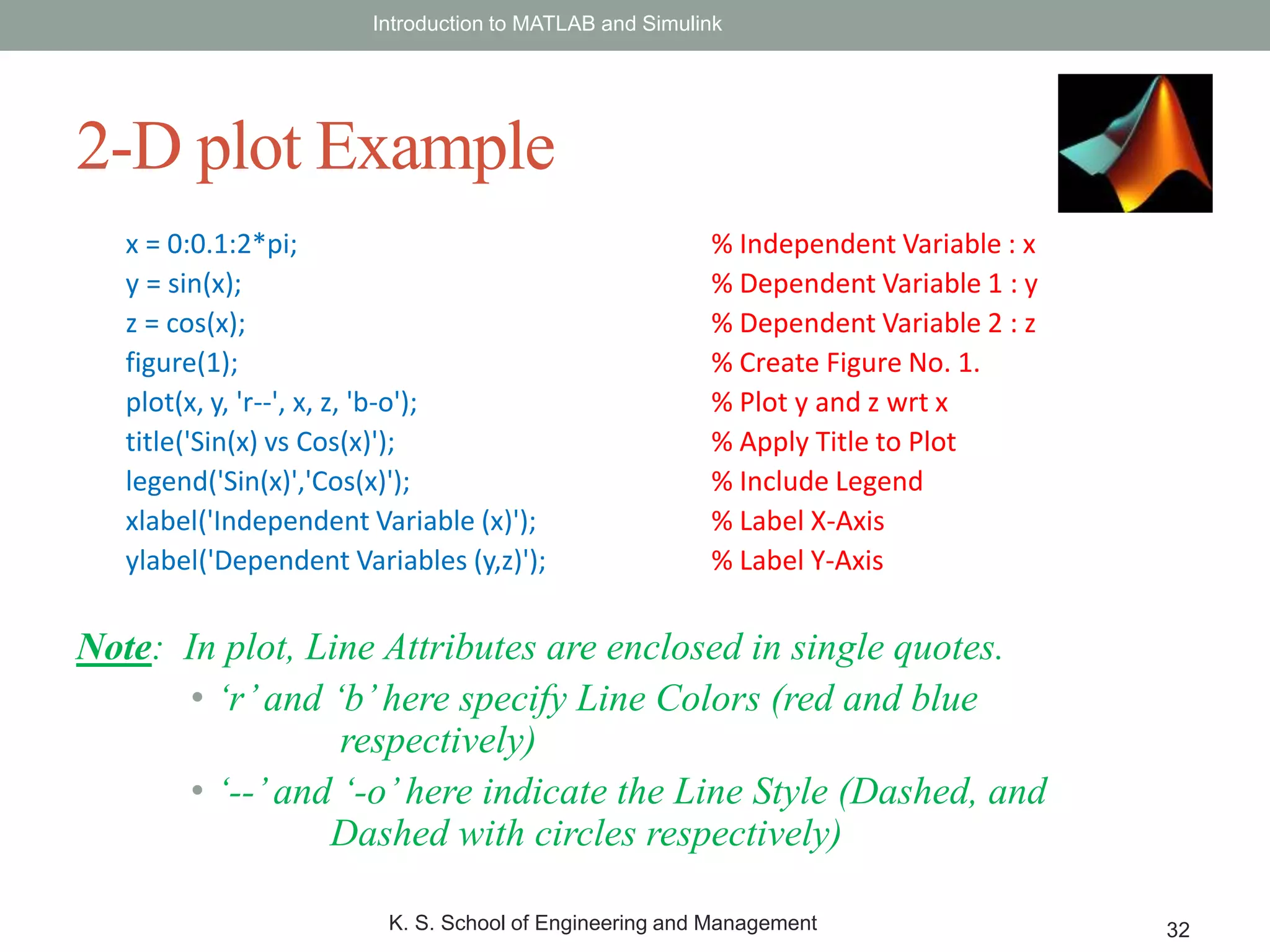
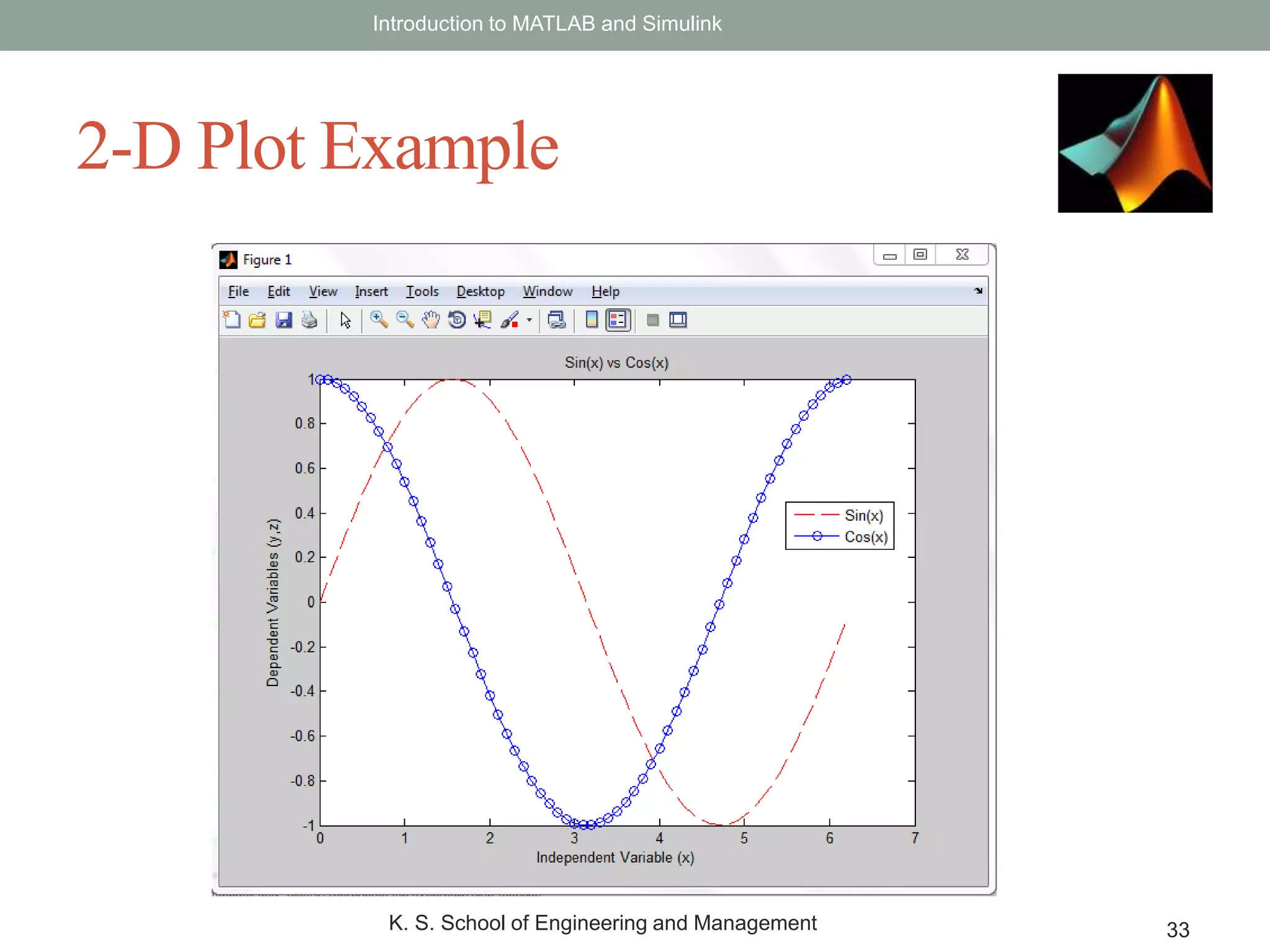
x = 0:0.1:2*pi; % Independent Variable : x
y = sin(x); % Dependent Variable 1 : y
z = cos(x); % Dependent Variable 2 : z
figure(1); % Create Figure No. 1.
plot(x, y, 'r--', x, z, 'b-o'); % Plot y and z wrt x
title('Sin(x) vs Cos(x)'); % Apply Title to Plot
legend('Sin(x)','Cos(x)'); % Include Legend
xlabel('Independent Variable (x)'); % Label X-Axis
ylabel('Dependent Variables (y,z)'); % Label Y-Axis
Note: In plot, Line Attributes are enclosed in single quotes.
• ‘r’and ‘b’here specify Line Colors (red and blue
respectively)
• ‘--’and ‘-o’here indicate the Line Style (Dashed, and
Dashed with circles respectively)
2-D plot Example

2-D Plot Example

• Syntax: title(‘String to be displayed’);
• This command adds the string contents to the Title.
>>title(['Hello. The value of pi = ',num2str(3.14159),' approximately']);
• Numerical content has to be first converted to string (num2str)
and then appended as a string.
• In order to append strings, we use the comma operator, and
enclose them within square brackets (remember, MATLAB sees
everything as vectors!)
• Backslash Operator () is used to include special characters (Eg.
alpha, beta, etc.)
Title of the Plot

• In case of multiple graphs in the same window, we use ‘legend’
to add legends, each corresponding to a separate graph/line.
• legend(‘label_1’, ‘label_2’, … , ‘label_n’);
• xlabel is used to label the X-axis, and ylabel is used to label the Y-
axis.
• LATEX conventions can be used here as well.
• for special characters, ^ for superscript and _ for subscript,
etc.
Axes Labels and Legend

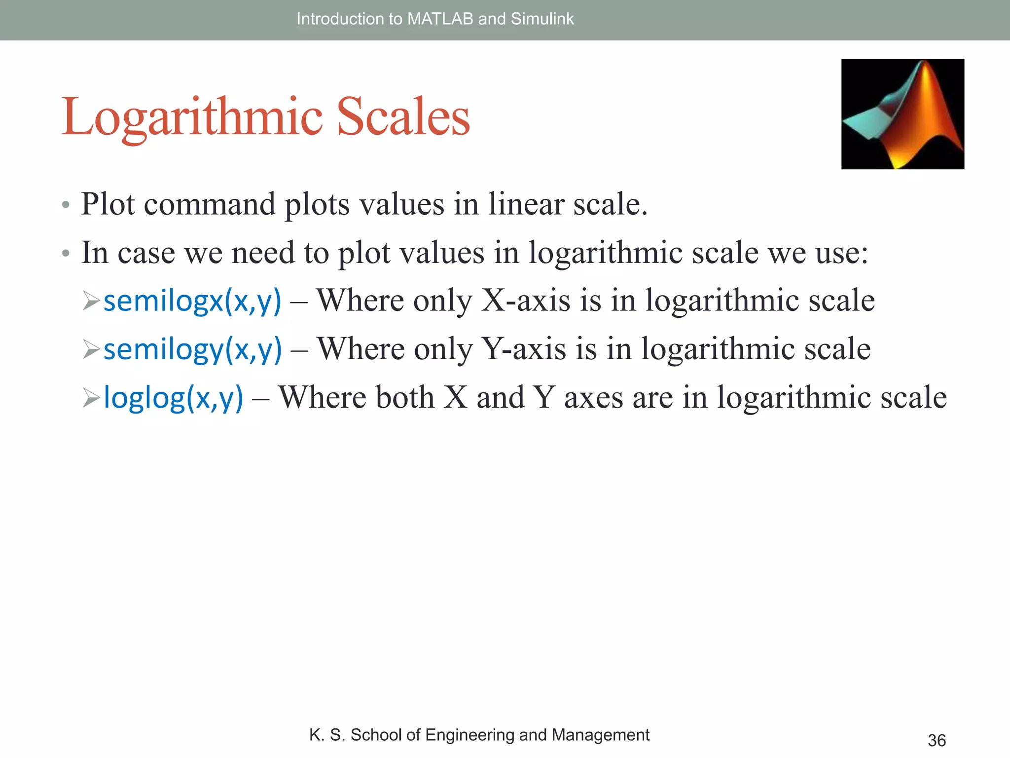
• Plot command plots values in linear scale.
• In case we need to plot values in logarithmic scale we use:
semilogx(x,y) – Where only X-axis is in logarithmic scale
semilogy(x,y) – Where only Y-axis is in logarithmic scale
loglog(x,y) – Where both X and Y axes are in logarithmic scale
Logarithmic Scales

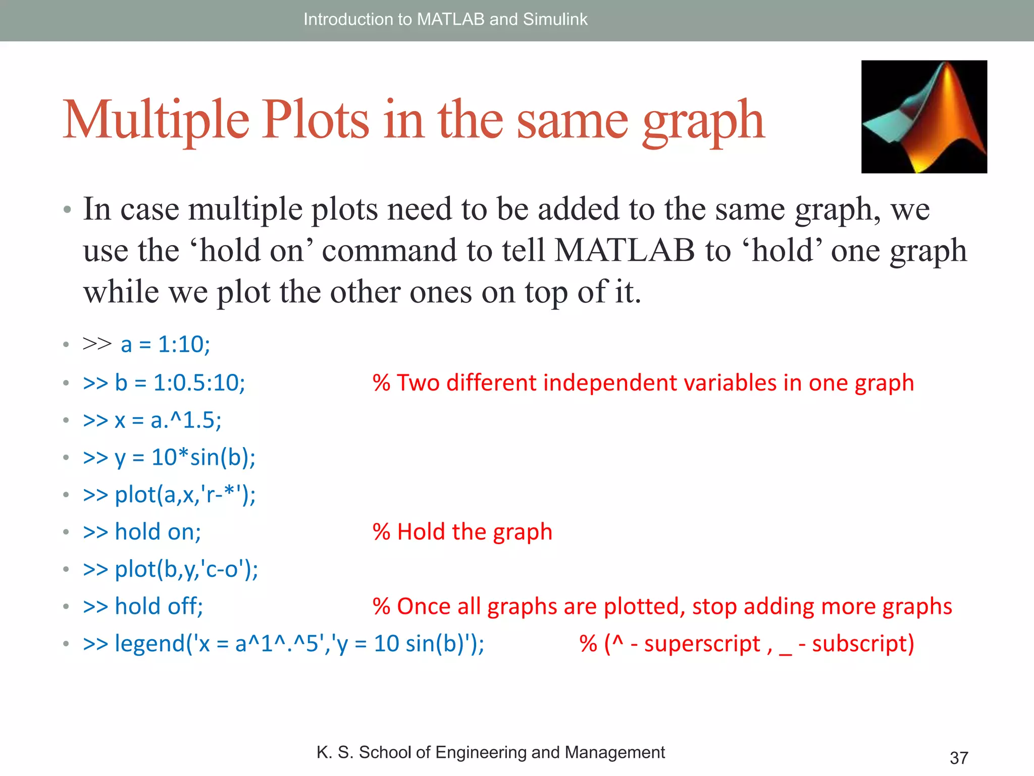
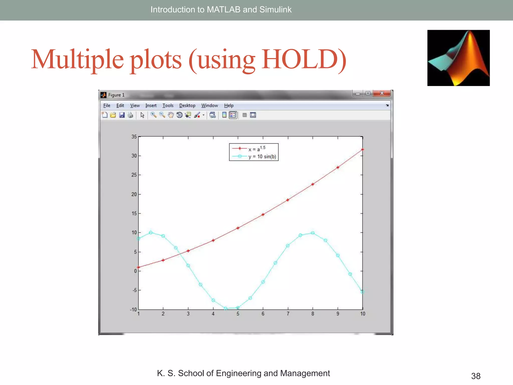
• In case multiple plots need to be added to the same graph, we
use the ‘hold on’ command to tell MATLAB to ‘hold’ one graph
while we plot the other ones on top of it.
• >> a = 1:10;
• >> b = 1:0.5:10; % Two different independent variables in one graph
• >> x = a.^1.5;
• >> y = 10*sin(b);
• >> plot(a,x,'r-*');
• >> hold on; % Hold the graph
• >> plot(b,y,'c-o');
• >> hold off; % Once all graphs are plotted, stop adding more graphs
• >> legend('x = a^1^.^5','y = 10 sin(b)'); % (^ - superscript , _ - subscript)
Multiple Plots in the same graph

Multiple plots (using HOLD)

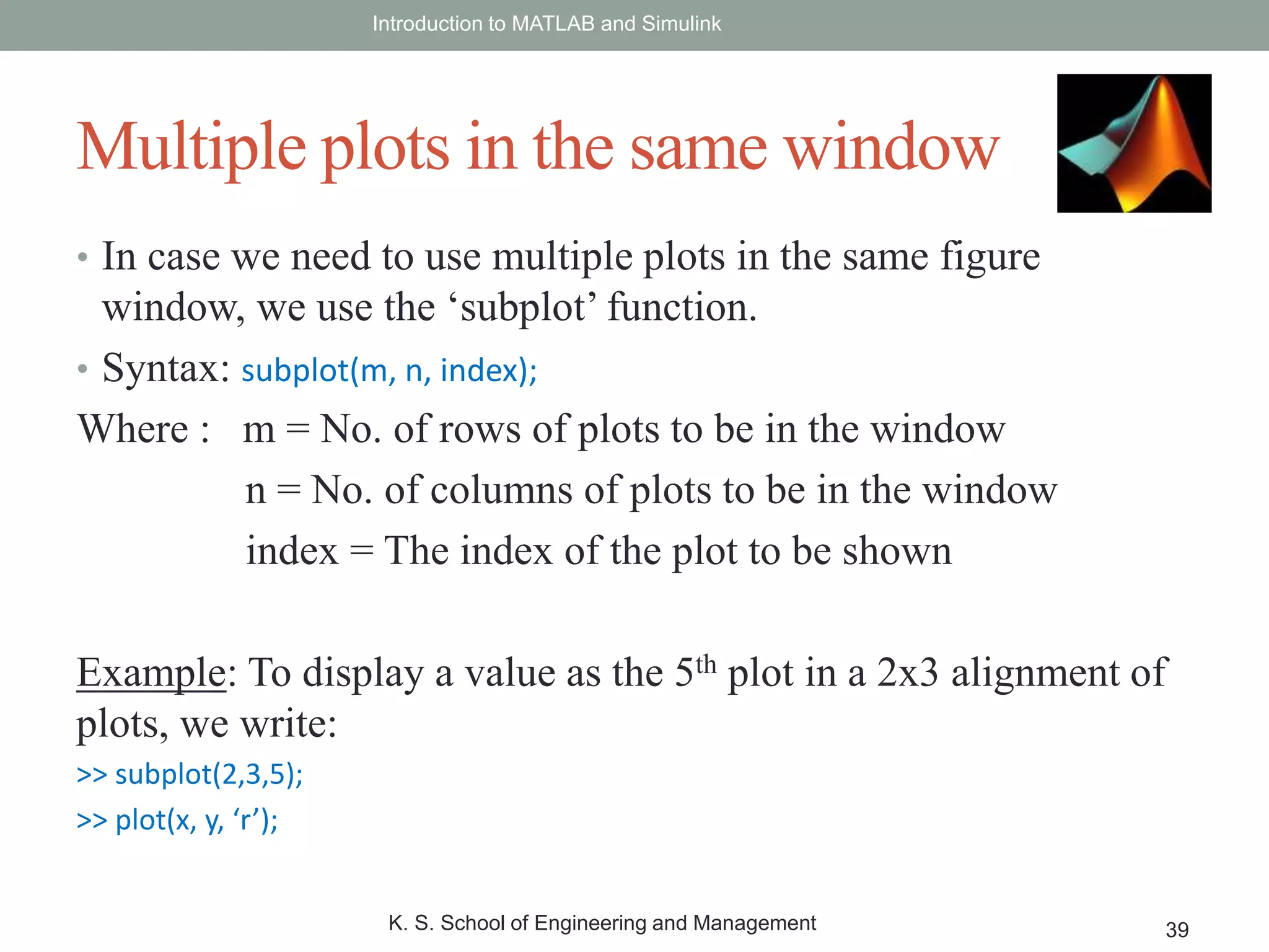
• In case we need to use multiple plots in the same figure
window, we use the ‘subplot’ function.
• Syntax: subplot(m, n, index);
Where : m = No. of rows of plots to be in the window
n = No. of columns of plots to be in the window
index = The index of the plot to be shown
Example: To display a value as the 5th plot in a 2x3 alignment of
plots, we write:
>> subplot(2,3,5);
>> plot(x, y, ‘r’);
Multiple plots in the same window

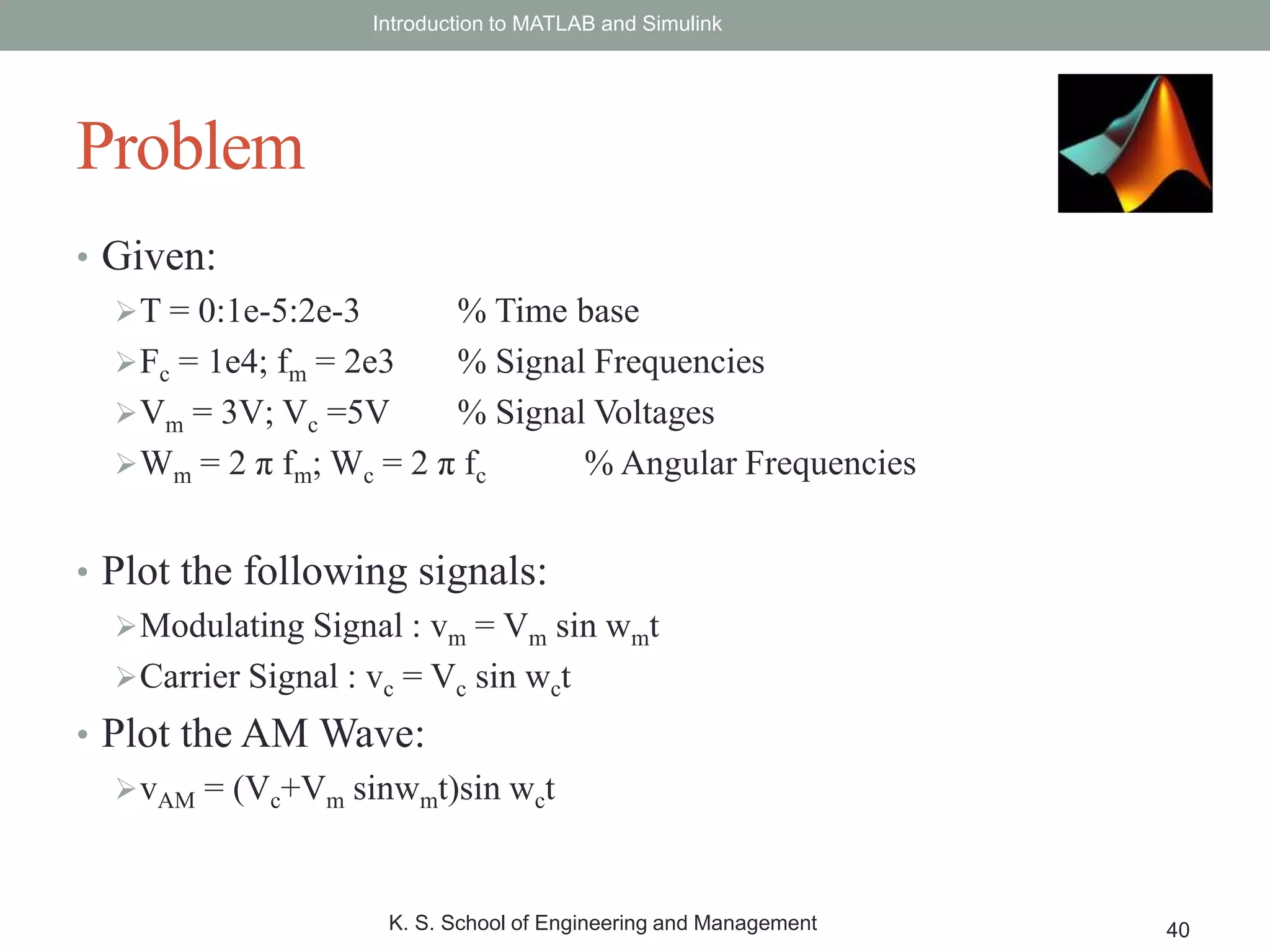
• Given:
T = 0:1e-5:2e-3 % Time base
Fc = 1e4; fm = 2e3 % Signal Frequencies
Vm = 3V; Vc =5V % Signal Voltages
Wm = 2 π fm; Wc = 2 π fc % Angular Frequencies
• Plot the following signals:
Modulating Signal : vm = Vm sin wmt
Carrier Signal : vc = Vc sin wct
• Plot the AM Wave:
vAM = (Vc+Vm sinwmt)sin wct
Problem

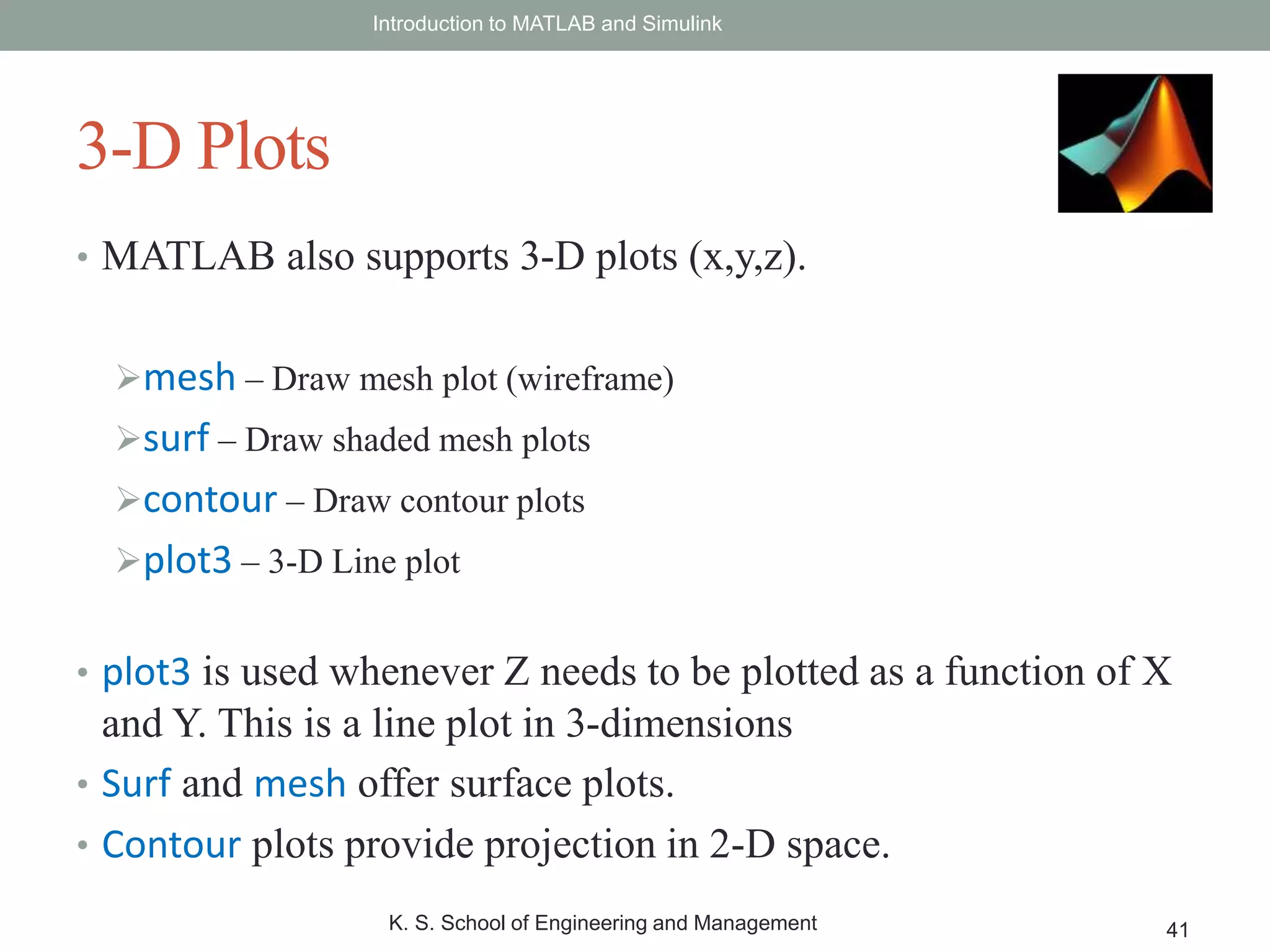
• MATLAB also supports 3-D plots (x,y,z).
mesh – Draw mesh plot (wireframe)
surf – Draw shaded mesh plots
contour – Draw contour plots
plot3 – 3-D Line plot
• plot3 is used whenever Z needs to be plotted as a function of X
and Y. This is a line plot in 3-dimensions
• Surf and mesh offer surface plots.
• Contour plots provide projection in 2-D space.
3-D Plots

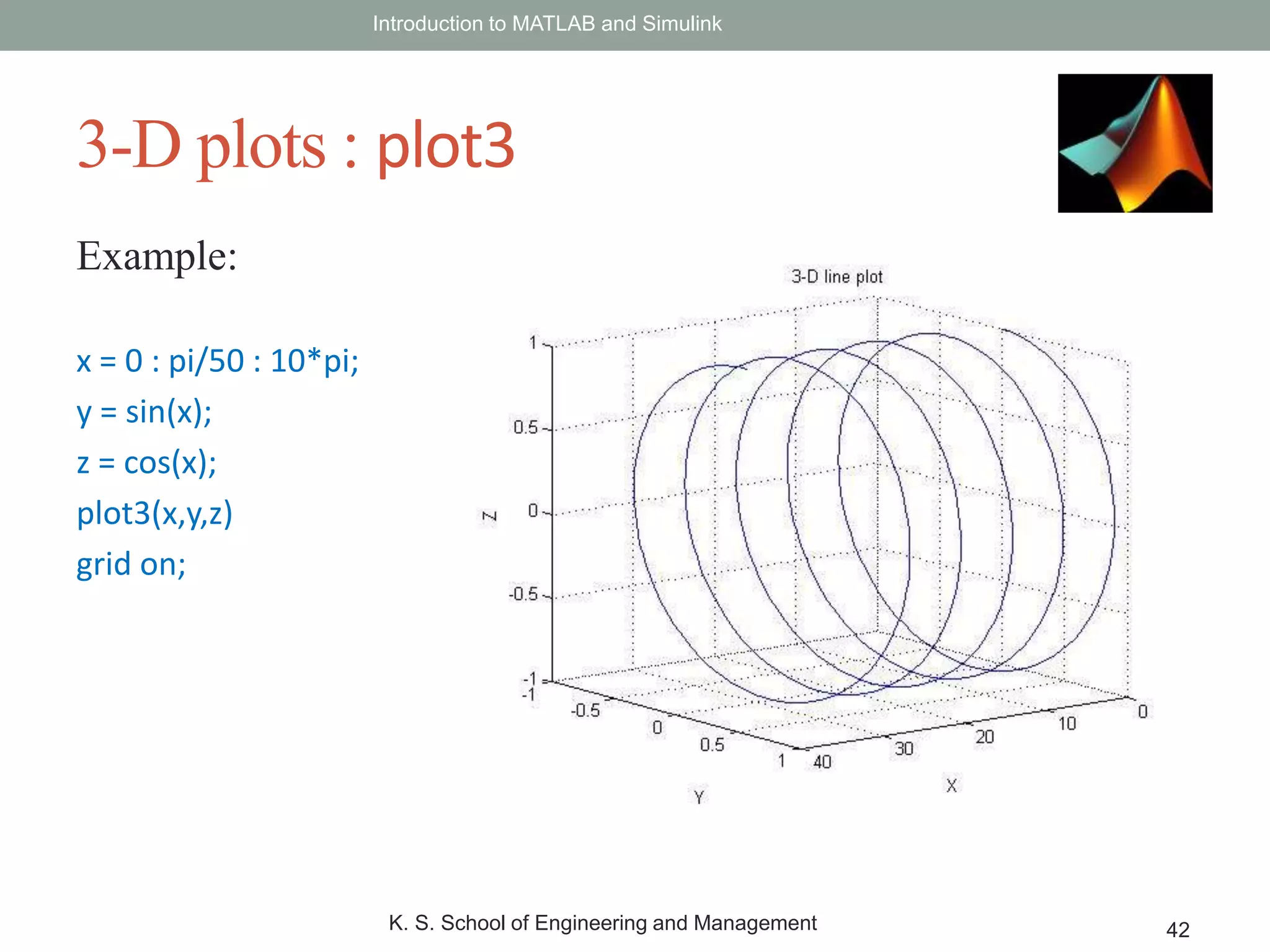
Example:
x = 0 : pi/50 : 10*pi;
y = sin(x);
z = cos(x);
plot3(x,y,z)
grid on;
3-D plots : plot3

• mesh is used to plot a wireframe plot of a variable z, which is a
function of two variables x and y. [z = f (x,y)]
• Surf is used to plot a surface map of z as a function of x and y.
• General syntax : surf(X, Y, Z)
mesh(X, Y, Z)
• If x is a (1 x m) sized vector, and y is a (1 x n) sized vector, the
z vector has to be of size (m x n).
• For every (x,y) pair, z has to have a corresponding value.
• meshgrid function can be used to create a 2-D or 3-D grid with
the given reference vector values.
3-D plots : mesh & surf

Example:
[X,Y] = meshgrid(-8:.5:8);
R = sqrt(X.^2 + Y.^2);
Z = sin(R)./R; %Sinc function
%Mesh Plot
subplot(2,1,1);
mesh(X,Y,Z);
% Surface Plot
subplot(2,1,2);
surf(X,Y,Z);
3-D plot : mesh & surf

• contour function generates a 2-D contour map, from 3-D space.
• Contours are color-mapped projection of 3-D surfaces onto 2-D
space.
• Example:
[X,Y,Z] = peaks(25);
figure(1);
subplot(2,1,1);
surf(X,Y,Z);
subplot(2,1,2);
contour(X,Y,Z);
Contour plots

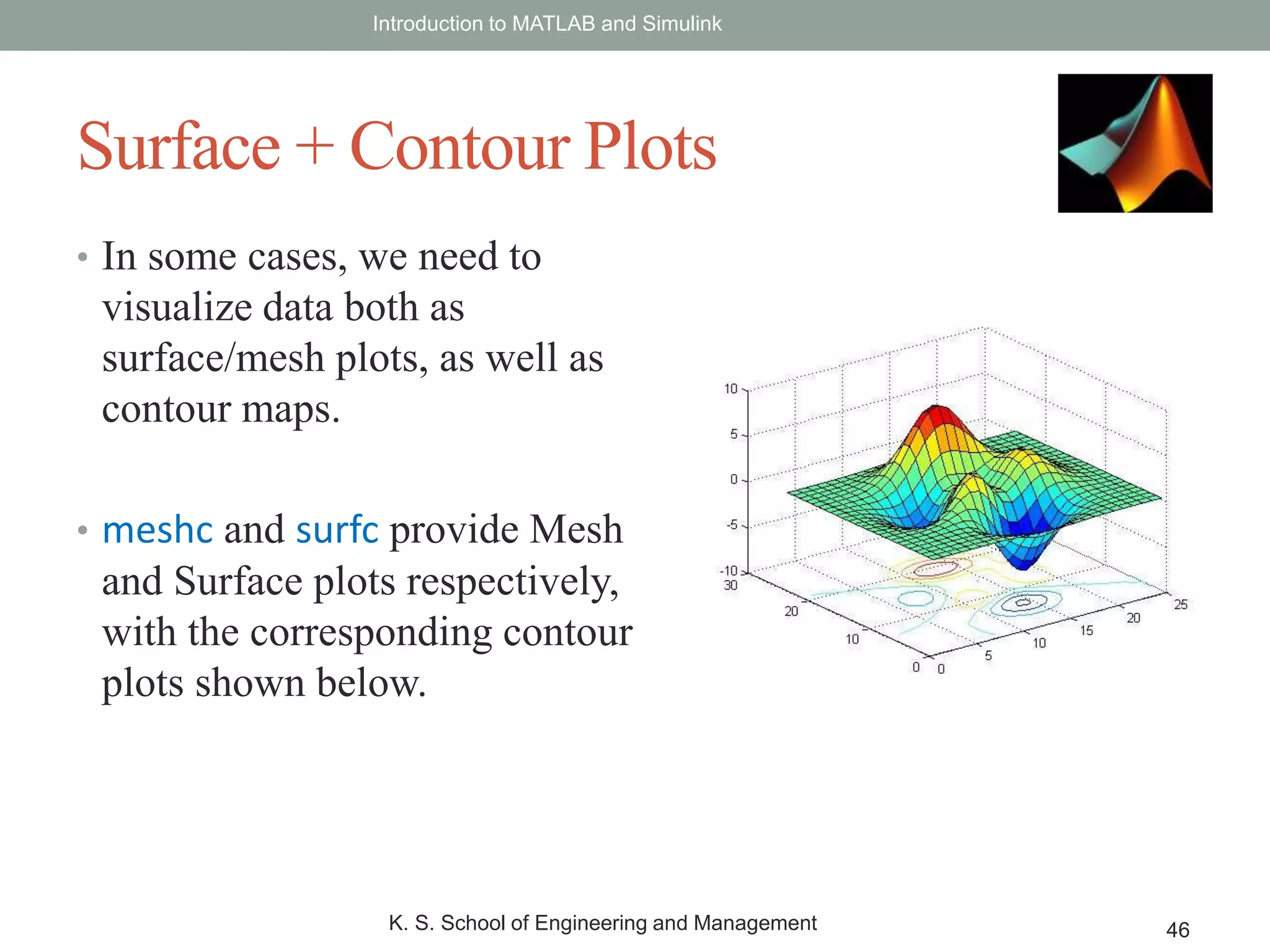
• In some cases, we need to
visualize data both as
surface/mesh plots, as well as
contour maps.
• meshc and surfc provide Mesh
and Surface plots respectively,
with the corresponding contour
plots shown below.
Surface + Contour Plots

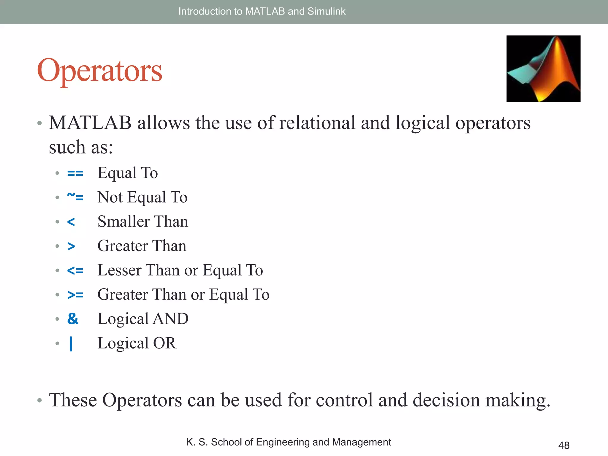
• MATLAB allows the use of relational and logical operators
such as:
• == Equal To
• ~= Not Equal To
• < Smaller Than
• > Greater Than
• <= Lesser Than or Equal To
• >= Greater Than or Equal To
• & Logical AND
• | Logical OR
• These Operators can be used for control and decision making.
Operators

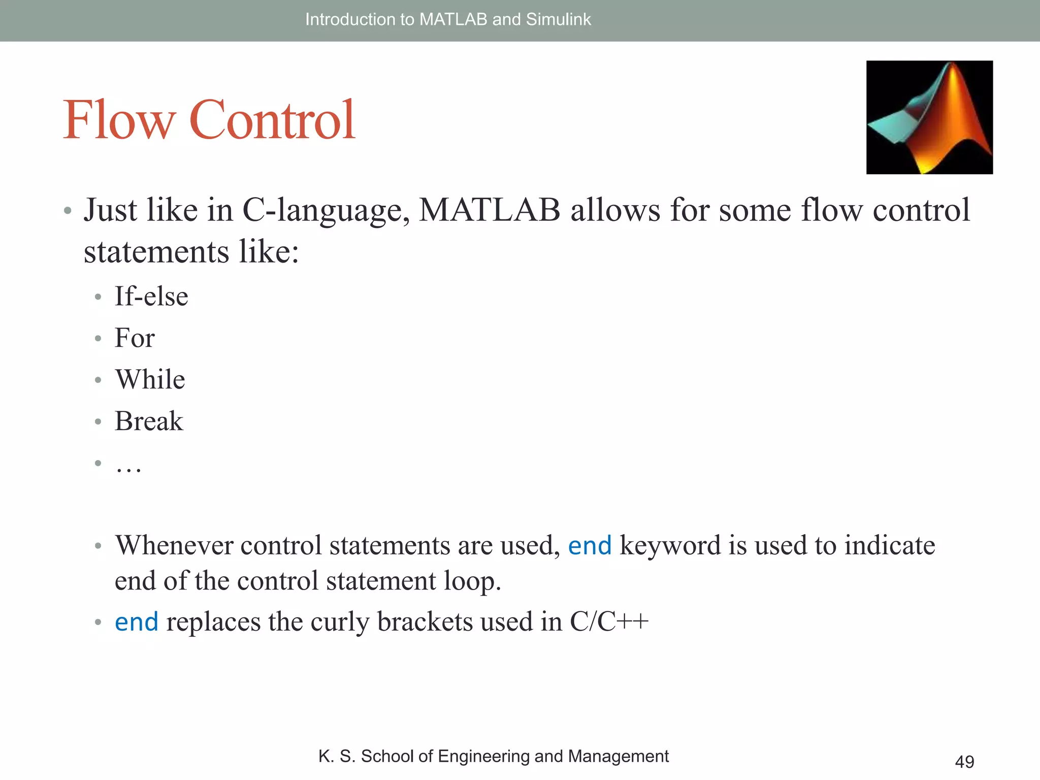
• Just like in C-language, MATLAB allows for some flow control
statements like:
• If-else
• For
• While
• Break
• …
• Whenever control statements are used, end keyword is used to indicate
end of the control statement loop.
• end replaces the curly brackets used in C/C++
Flow Control

• Syntax:
if(condition_1)
Commands_1
elseif(condition_2)
Commands_2
elseif(condition_3)
Commands_3
else
Commands_n
end
Control Structure : if-else
• Example:
If((a>3) &(b<5))
x = [1 0];
elseif(((b==5))
x = [1 1];
else
x = [0 1];
end

• Syntax:
for i = index_array
Matlab Commands;
end
Control Structure: for
• Examples:
for i = -1 : 0.01 : 1
x = i^2+sin(i);
end
or
for k = [0.2 0.4 0.1 0.8 1.3]
y = sin(k);
end

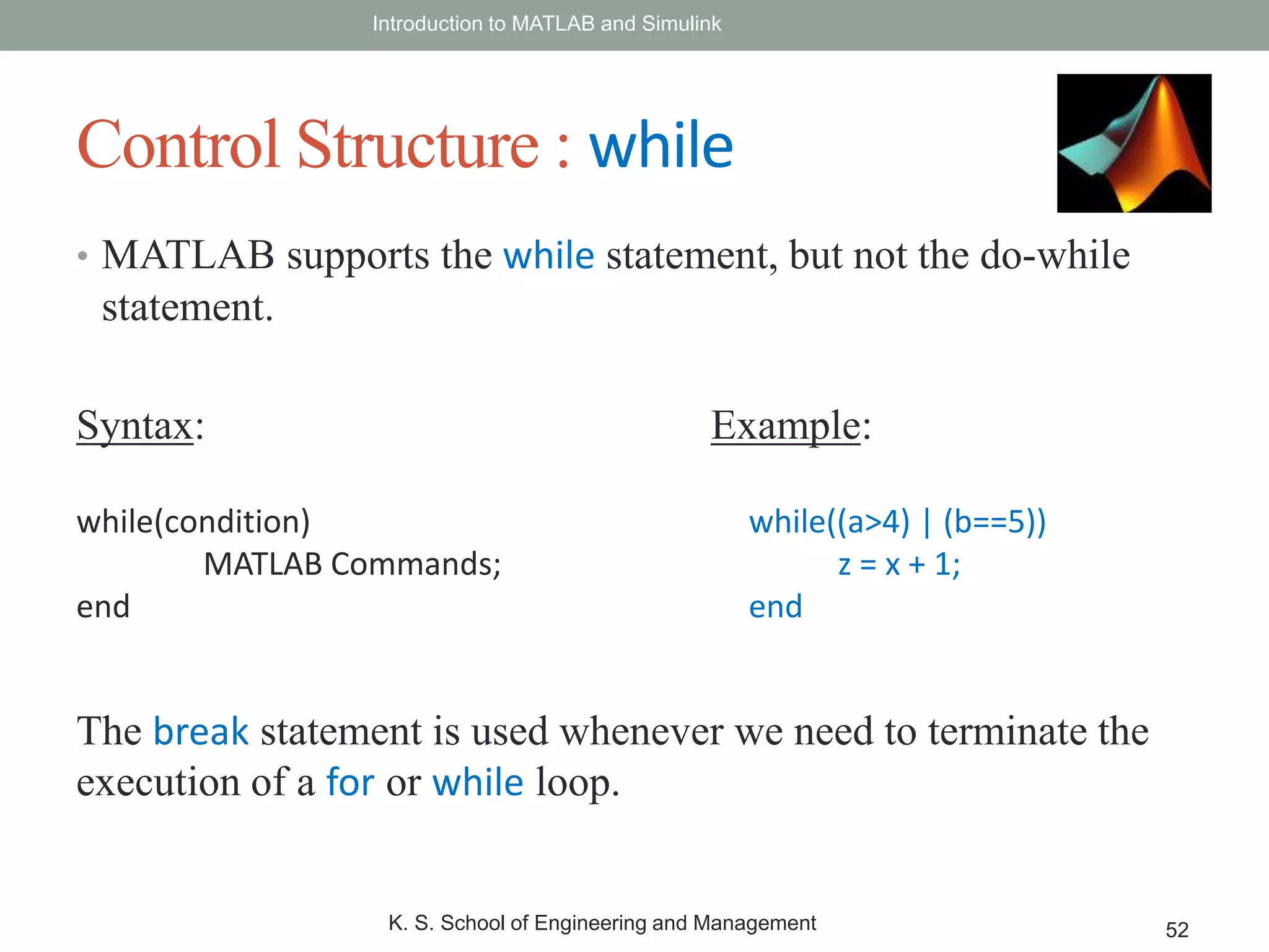
• MATLAB supports the while statement, but not the do-while
statement.
Control Structure : while
Syntax:
while(condition)
MATLAB Commands;
end
Example:
while((a>4) | (b==5))
z = x + 1;
end
The break statement is used whenever we need to terminate the
execution of a for or while loop.

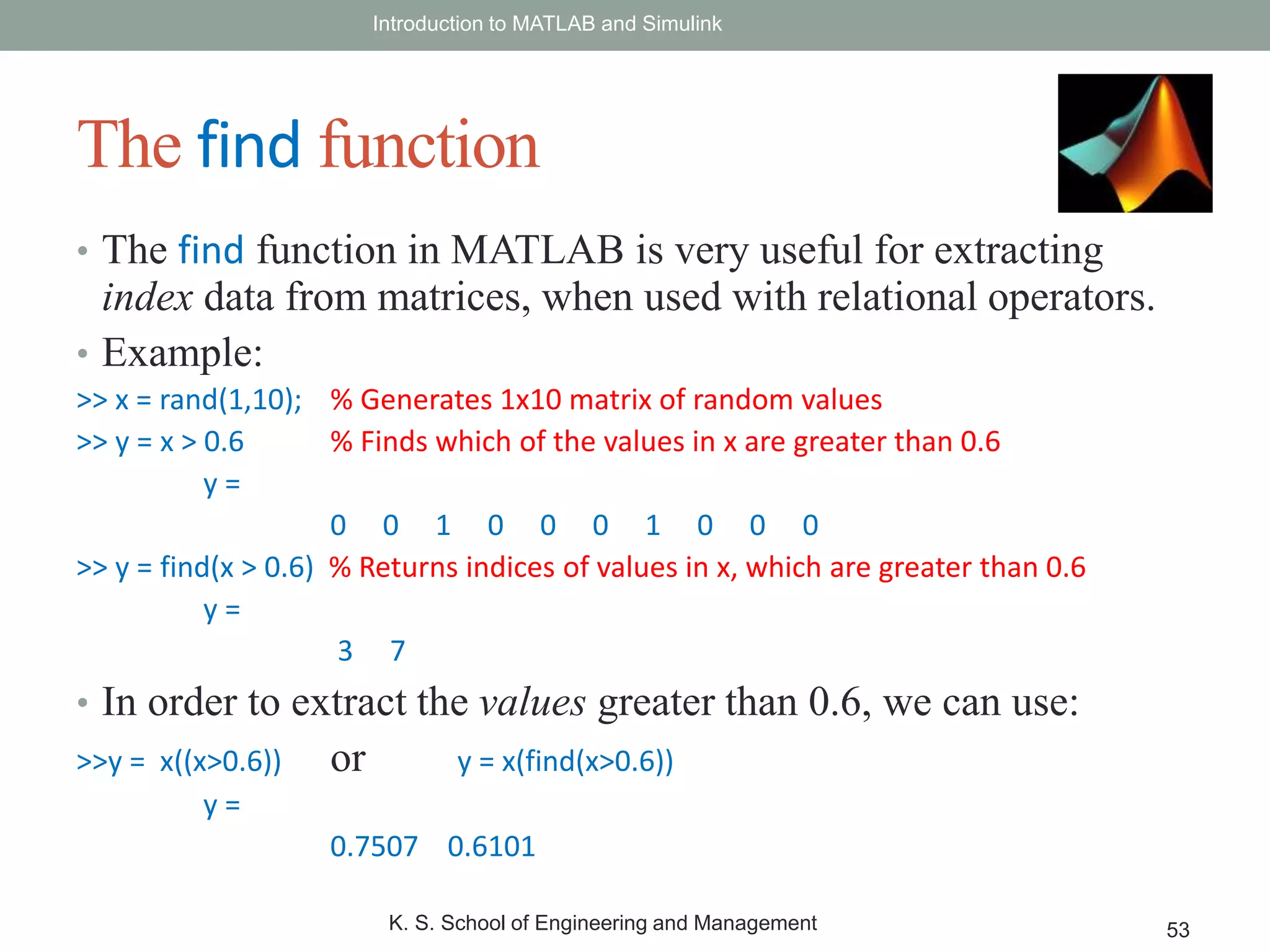
• The find function in MATLAB is very useful for extracting
index data from matrices, when used with relational operators.
• Example:
>> x = rand(1,10); % Generates 1x10 matrix of random values
>> y = x > 0.6 % Finds which of the values in x are greater than 0.6
y =
0 0 1 0 0 0 1 0 0 0
>> y = find(x > 0.6) % Returns indices of values in x, which are greater than 0.6
y =
3 7
• In order to extract the values greater than 0.6, we can use:
>>y = x((x>0.6)) or y = x(find(x>0.6))
y =
0.7507 0.6101
The find function

• Scripts are programs written for interpreters (as opposed to
compilers)
• Scripts automate execution of tasks for a particular application.
• MATLAB scripts are based on C-language syntax
• % symbol is used for single line comments.
• MATLAB does not support multiline commenting.
• MATLAB scripts can be divided into independently-executable
sections using the %% symbol (Section Breaks). This is very
useful for larger programs with multiple sections.
• Scripts are stored with a .m file extension.
MATLAB Scripts

ASimple Script

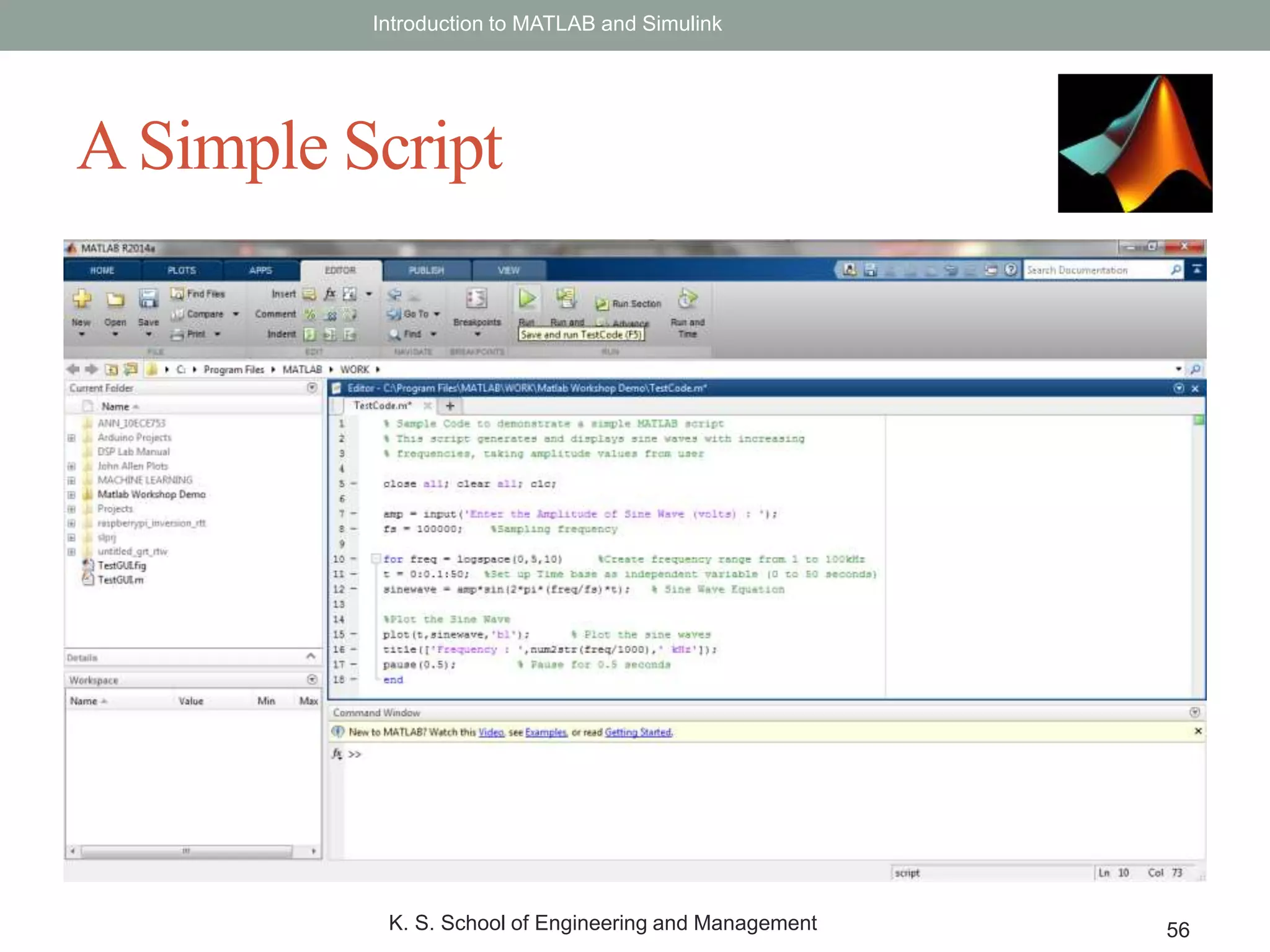
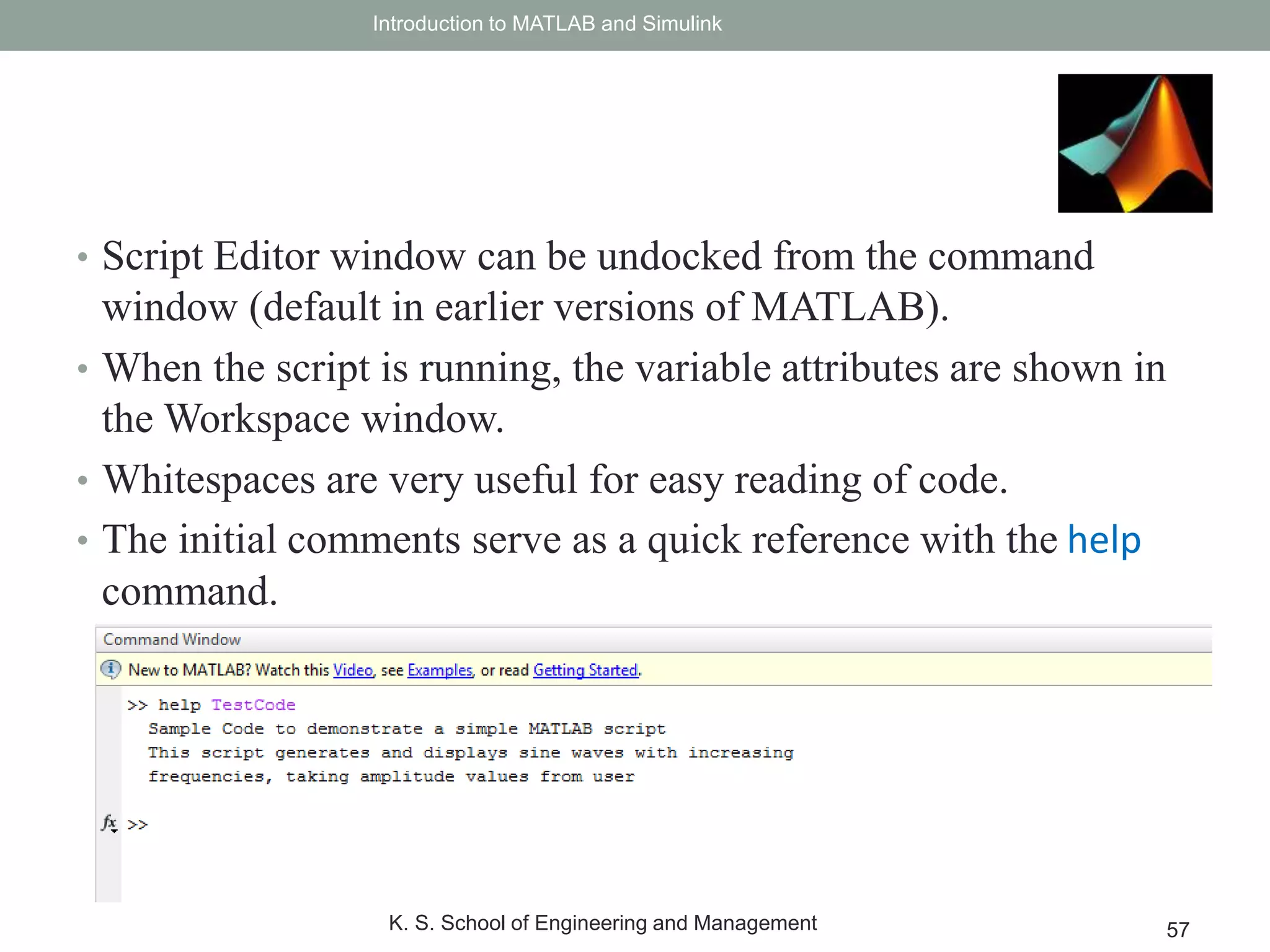
• Script Editor window can be undocked from the command
window (default in earlier versions of MATLAB).
• When the script is running, the variable attributes are shown in
the Workspace window.
• Whitespaces are very useful for easy reading of code.
• The initial comments serve as a quick reference with the help
command.

• Whenever we have huge programs, with repeated operations, it
is preferable to use functions.
• Functions make code more readable and compact.
• Functions speed up processing, and simplify the code.
• MATLAB functions are indicated by a keyword function, and
can handle multiple variables.
• MATLAB Functions are of three types:
• Inline Functions
• Anonymous Functions
• Standalone Functions
MATLAB Functions

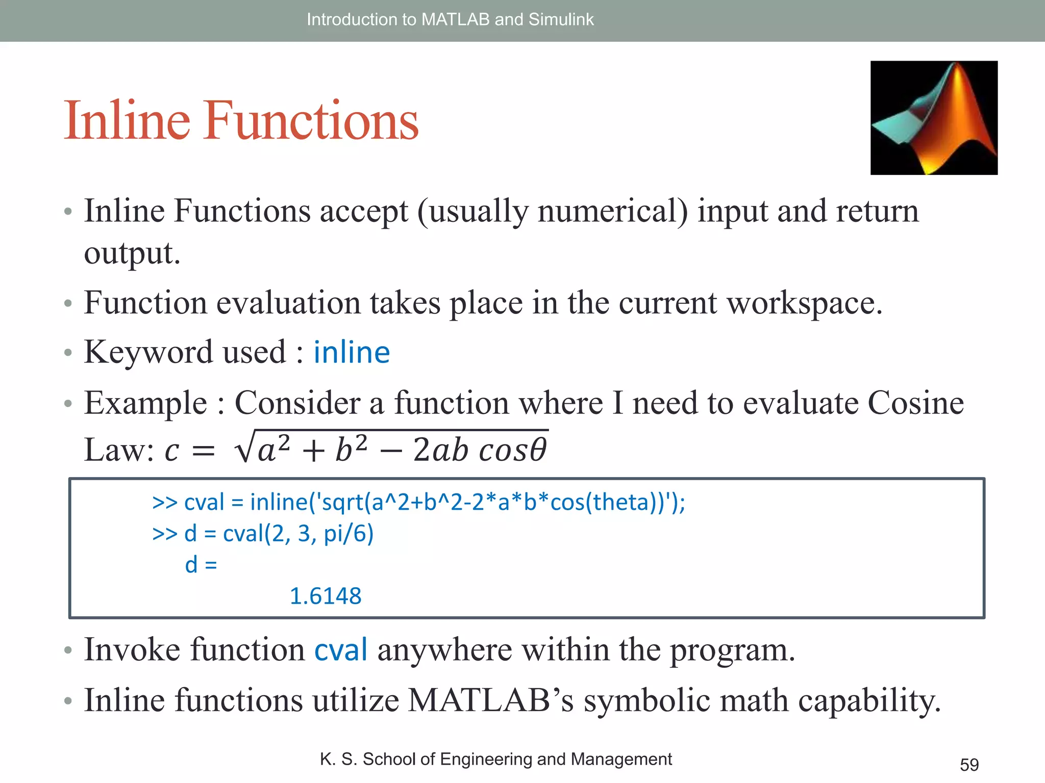
• Inline Functions accept (usually numerical) input and return
output.
• Function evaluation takes place in the current workspace.
• Keyword used : inline
• Example : Consider a function where I need to evaluate Cosine
Law: 𝑐 = 𝑎2 + 𝑏2 − 2𝑎𝑏 𝑐𝑜𝑠𝜃
• Invoke function cval anywhere within the program.
• Inline functions utilize MATLAB’s symbolic math capability.
Inline Functions
>> cval = inline('sqrt(a^2+b^2-2*a*b*cos(theta))');
>> d = cval(2, 3, pi/6)
d =
1.6148

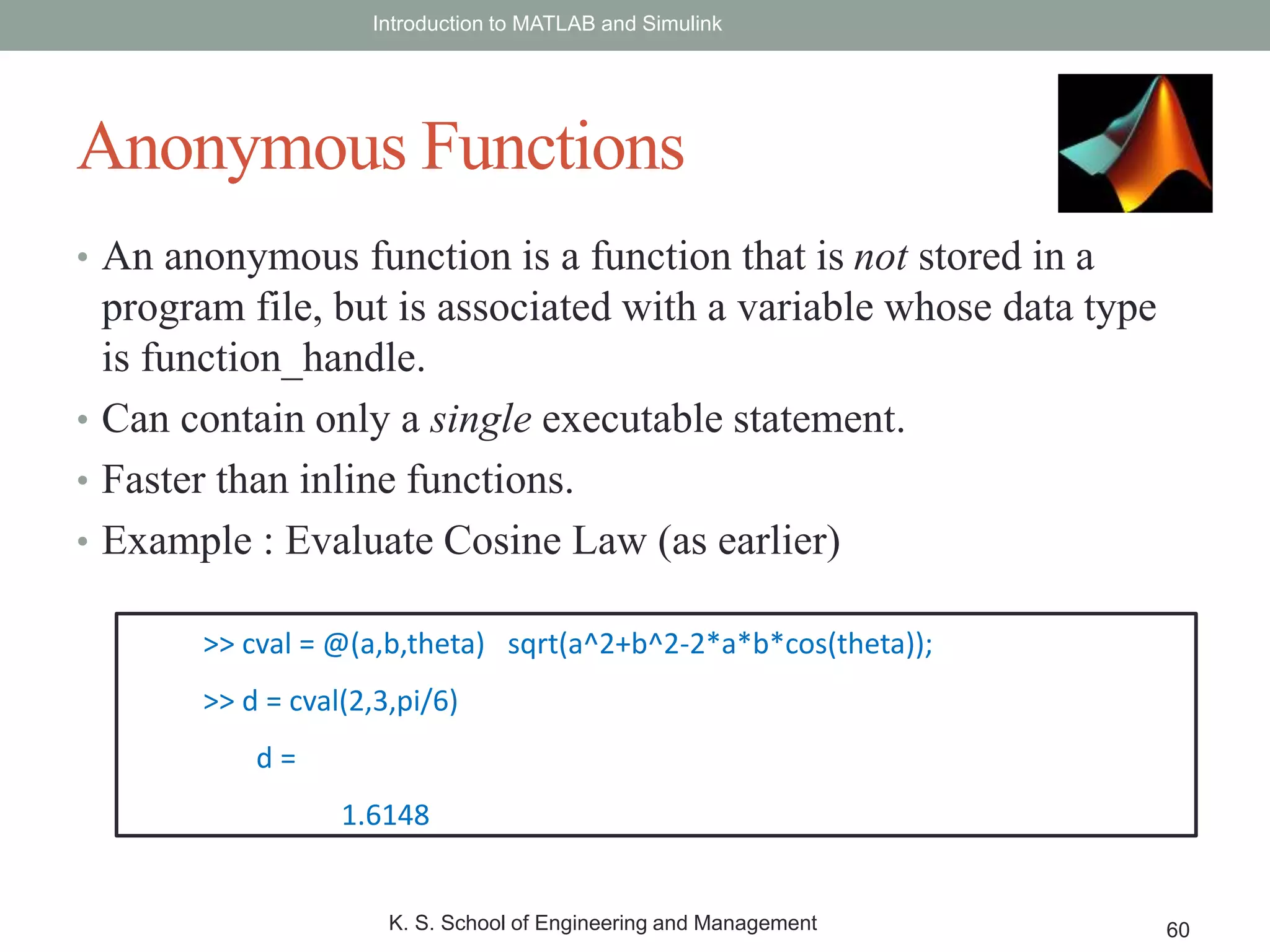
• An anonymous function is a function that is not stored in a
program file, but is associated with a variable whose data type
is function_handle.
• Can contain only a single executable statement.
• Faster than inline functions.
• Example : Evaluate Cosine Law (as earlier)
Anonymous Functions
>> cval = @(a,b,theta) sqrt(a^2+b^2-2*a*b*cos(theta));
>> d = cval(2,3,pi/6)
d =
1.6148

• Commands executed in a separate workspace which is created
whenever the function is called.
• Function files are saved with the same name as the function,
with a .m extension.
• During function calls, input and output arguments have to be
specified.
• The first (command) line of a Function M-file MUST be a
function declaration line specifying input and ouput variables.
• Make sure that no undefined variable occurs as input to these
commands!
Function Files

• File name : quadroots.m
• Calling the function quadroots
Function File Example
function [root1,root2] = quadroots(a,b,c)
%quadroots calculates the roots of the quadratic equation given by:
% f(x) = ax^2+bx+c
% Given the coefficients a,b,c as input.
root1 = (-b+sqrt(b.^2-4.*a.*c))/(2.*a);
root2 = (-b-sqrt(b.^2-4.*a.*c))/(2.*a);
end
>> [r1,r2] = quadroots(3,4,2)
r1 =
-0.6667 + 0.4714i
r2 =
-0.6667 - 0.4714i

1. Create a function that generates the factorial of a given
number.
Problem

• MATLAB variables and data can be imported from and
exported to a variety of formats including:
• MATLAB formatted data (.mat)
• Text (csv, txt, delimited data)
• Spreadsheets (xls, xlsx, xlsm, ods)
• Extensible Markup Language (xml)
• Scientific Data (cdf, fits, hdf, h5, nc)
• Image (bmp, jpg, png,tiff,gif, pbm, pcf, ico, etc)
• Audio (au, snd, flac, ogg, wav, m4a, mp4, mp3, etc)
• Video (avi, mpg, wmv, asf, mp4, mov, etc)
Import and Export of Data

• Depending on the type of files containing the data, different
MATLAB commands can be used to import or export data.
• Data import/export can be done in two ways:
• Commands in Command Line
• Right Click and Import/Export from Workspace/Command Window
• While importing or exporting data from scripts, we generally
use the MATLAB commands.
• Right Click actions are used whenever we are importing data
from or exporting data to files, while working in the Command
window.
Import/Export

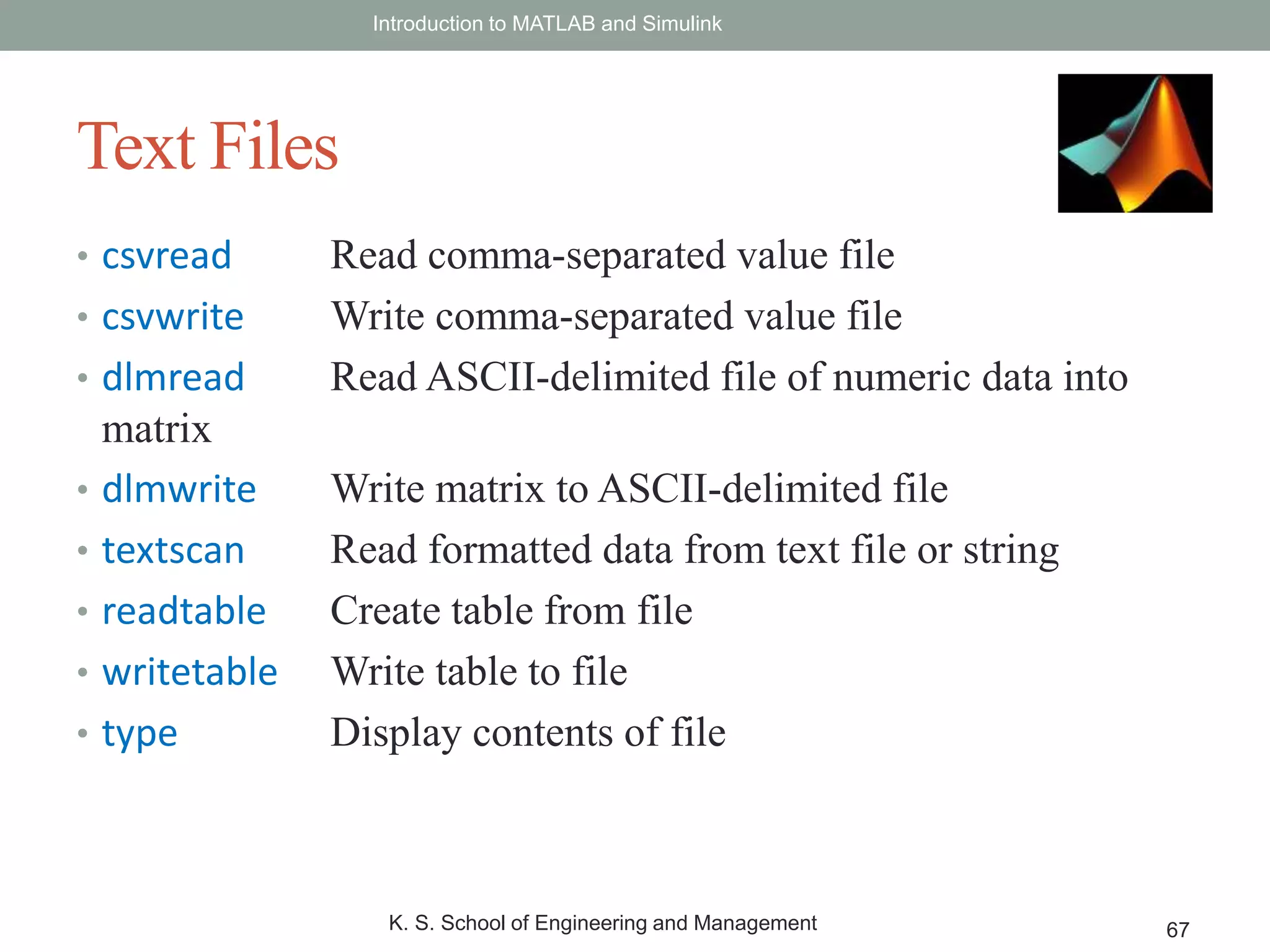
• csvread Read comma-separated value file
• csvwrite Write comma-separated value file
• dlmread Read ASCII-delimited file of numeric data into
matrix
• dlmwrite Write matrix to ASCII-delimited file
• textscan Read formatted data from text file or string
• readtable Create table from file
• writetable Write table to file
• type Display contents of file
Text Files

Consider a text file Delhitemp.txt, containing daily average
temperature data for 20 years (Month-Day-Year-Temp format)
We See that C is now a structure with 4 fields:
C =
[7125x1 int32] [7125x1 int32] [7125x1 int32] [7125x1 double]
Now, I can assign the values to individual fields :
>>TempVals = C{4} % { } accesses MATLAB ‘cell’ elements
Now, TempVals is a 7125x1 matrix of floating point values.
Text Import (.txt)
>> cd('C:UsersRaviDesktopmatlab workshop filesDataset files');
>> fname = 'Delhitemp.txt'; % Name of file in current directory
>> fileID = fopen(fname,'r'); % Open file, (r)ead only
>> fileSpecs = '%d%d%d%f'; %Data format – int, int, int, float
>> C = textscan(fileID,filespecs,'HeaderLines',1); %Scan text and extract data

• Let’s try plotting the temperature variation for the past 20 years!
>>plot(TempVals);
title(['Temperature Variations from ',num2str(C{3}(1,:)), ' to ', num2str(C{3}(end,:))]);
xlabel('Days');
ylabel('Temperature (F)');
Note: C{3}(1,:) accesses the
first row and all columns (to
extract the complete string)
of Cell C’s field no. 3 (Year)
Similarly, C{3}(end,:),
extracts the last year value
in the same field.

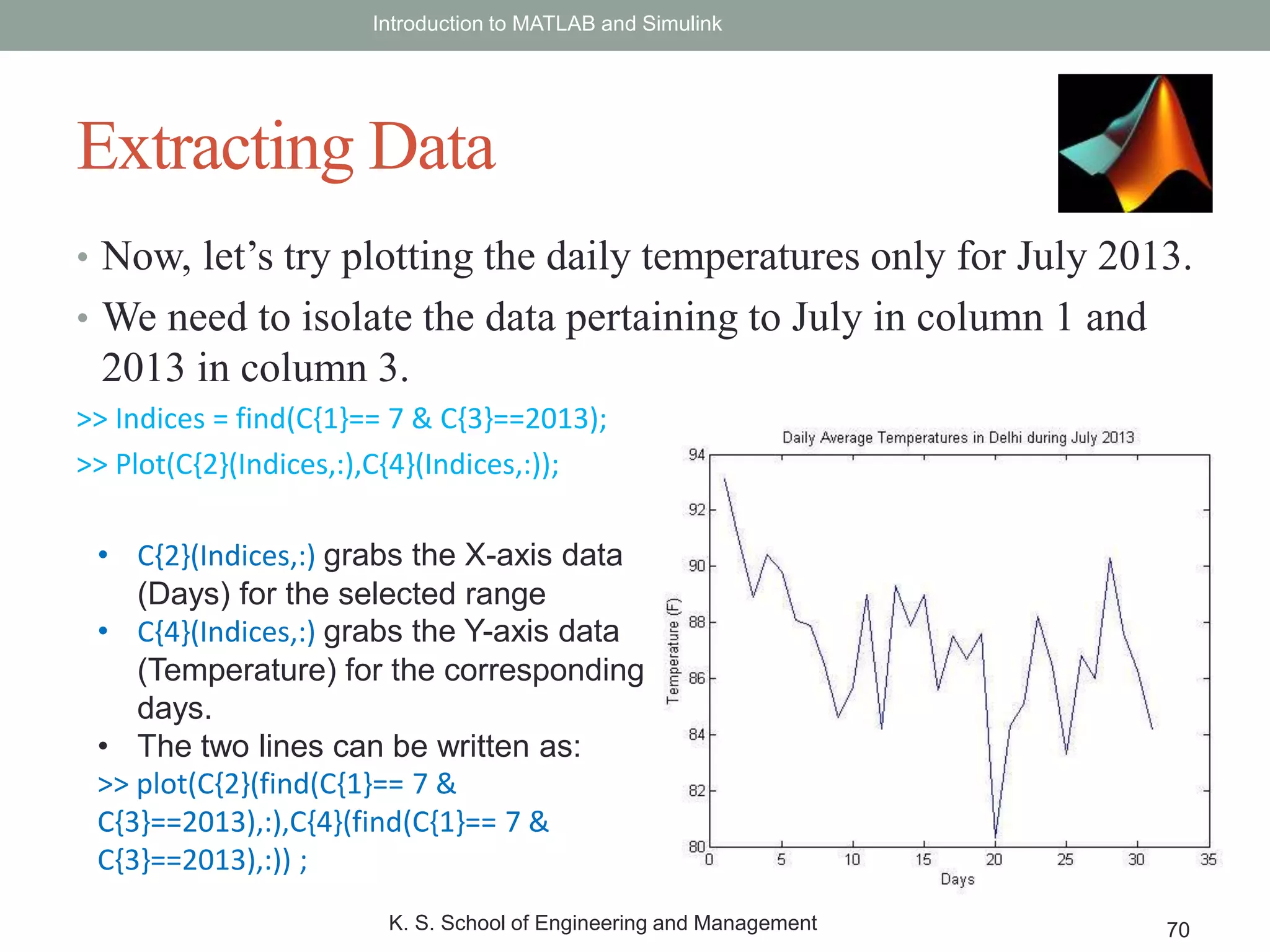
• Now, let’s try plotting the daily temperatures only for July 2013.
• We need to isolate the data pertaining to July in column 1 and
2013 in column 3.
>> Indices = find(C{1}== 7 & C{3}==2013);
>> Plot(C{2}(Indices,:),C{4}(Indices,:));
Extracting Data
• C{2}(Indices,:) grabs the X-axis data
(Days) for the selected range
• C{4}(Indices,:) grabs the Y-axis data
(Temperature) for the corresponding
days.
• The two lines can be written as:
>> plot(C{2}(find(C{1}== 7 &
C{3}==2013),:),C{4}(find(C{1}== 7 &
C{3}==2013),:)) ;

• Most databases store data in CSV format (Comma Separated
Value), where the comma is the delimiter.
• MATLAB’s csvread function makes importing CSV data easy.
• Syntax: X = csvread(‘filename.csv’, row, col);
• Here, Row and Col indicate the row and column number from
which scanning has to commence. (zero based)
• In case the CSV files have headers, titles, explanations, etc, we
can skip those lines from the files and point the (Row, Col)
values to the cell where the data begins.
• Once the import is done, X becomes a matrix of values where
data is stored.
.csv files

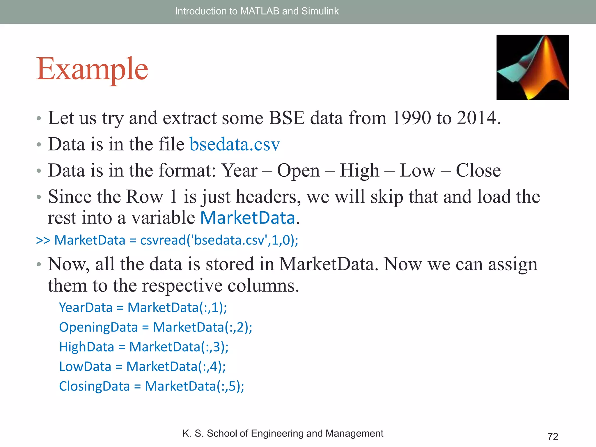
• Let us try and extract some BSE data from 1990 to 2014.
• Data is in the file bsedata.csv
• Data is in the format: Year – Open – High – Low – Close
• Since the Row 1 is just headers, we will skip that and load the
rest into a variable MarketData.
>> MarketData = csvread('bsedata.csv',1,0);
• Now, all the data is stored in MarketData. Now we can assign
them to the respective columns.
YearData = MarketData(:,1);
OpeningData = MarketData(:,2);
HighData = MarketData(:,3);
LowData = MarketData(:,4);
ClosingData = MarketData(:,5);
Example

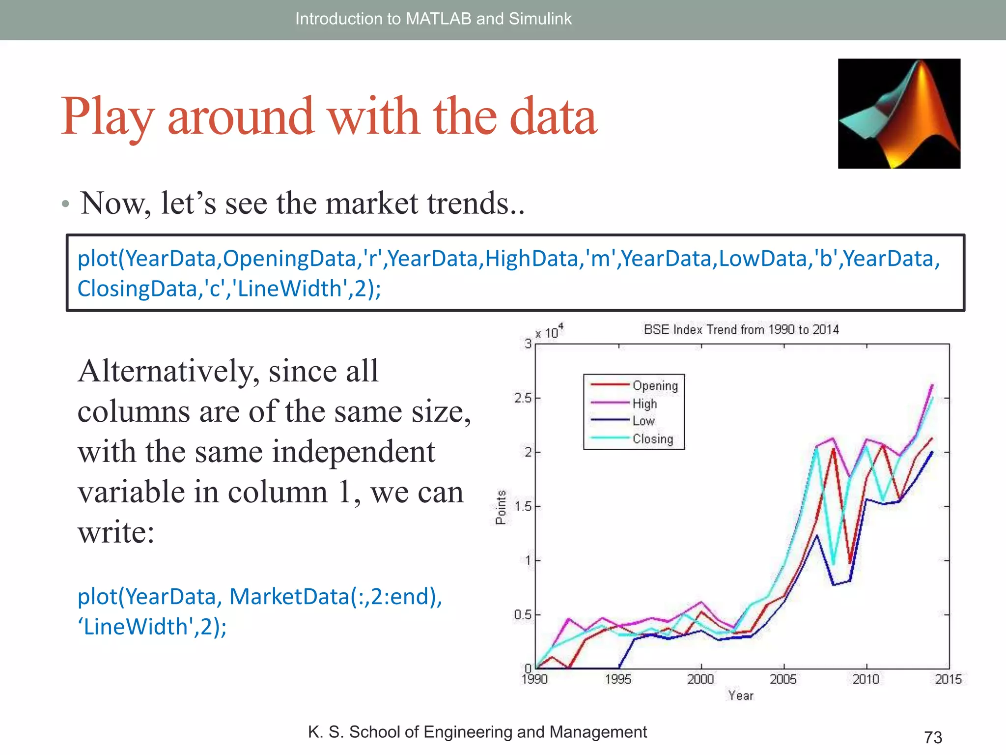
• Now, let’s see the market trends..
Play around with the data
plot(YearData,OpeningData,'r',YearData,HighData,'m',YearData,LowData,'b',YearData,
ClosingData,'c','LineWidth',2);
Alternatively, since all
columns are of the same size,
with the same independent
variable in column 1, we can
write:
plot(YearData, MarketData(:,2:end),
‘LineWidth',2);

• MATLAB variables can be exported into csv format for use
with other applications too.
• This is achieved using the csvwrite function:
• Syntax : csvwrite(‘filename’, Variable, Row, Col)
• Example : If I want to write just the Opening and Closing
values from my data set, to a csv file named
‘BSEOpenClose.csv’:
• >> csvwrite('BSEopenclose.csv',[YearData OpeningData ClosingData],1,0);
• The file BSEopenclose.csv is written into the current directory,
and contains the year, Closing Data and Opening Data, with
data being written starting from 2nd row.
Writing to csv files

• In case data is stored in Excel Spreadsheets, MATLAB can
extract data from that too.
• xlsread is used to read Excel Spreadsheets and extract data from
it.
• xlsread can extract data from all pages or from a specified set of
pages.
• xlswrite can be used to write MATLAB workspace variables
and data into Excel Spreadsheets.
.xls and .xlsx files

• Syntax : num = xlsread(filename,sheet,xlRange);
• Filename – String enclosed in quotes
• Sheet – Worksheet number
• xlRange – Range of cell values to be imported
• Example : tempData = xlsread('IndMinTemp.xls', 'A3:F114');
• This reads all values in the spreadsheet from Page 1 (as not
specified), and from cells A3 through F114.
Importing Excel data

• Syntax : Status = xlswrite(filename,A,sheet,xlRange)
• Filename – Name of the Excel File to be created.
• A – Matrix/Vector to be stored in the Spreadsheet
• Sheet – Sheet Number in the workbook
• xlRange – Range of cells in which data is to be stored.
• Status – 1 if successful, 0 in case of failure.
• Example: To save a variable Num in an excel sheet named
“numericalvalue.xlsx’:
Status = xlswrite(‘numericalvalue.xlsx’, Num)
Exporting to Excel

• Get the spreadsheet file : Monthly_And_Annual_Rainfall.xls
• Extract data into the workspace.
• Plot the annual rainfall values for any 5 cities from 1951 to
2012, clearly indicating the cities.
• Plot the seasonal rainfall for the same 5 cities for the year 1980
in another graph.
Problem

• MathWorks®, MATLAB®, Simulink® and the Mathworks Logo
are all trademarks or registered trademarks of The MathWorks,
Inc.
Acknowledgment

Introduction to MATLAB

In this document

More Related Content

What's hot

Similar to Introduction to MATLAB

Recently uploaded

Introduction to MATLAB