Interpretation and Utilization of Assessment Results.docx

Prepared by:
Interpretation and Utilization of Assessment Results
MODULE 4

LEARNING OUTCOMES
1. Construct frequency distribution based on a given set of
scores.
2. Apply statistics to calculate and compare individual and
group scores.
3. Distinguish the measures of central tendency from the
measures of variation.
4. Describe and interpret assessment results.

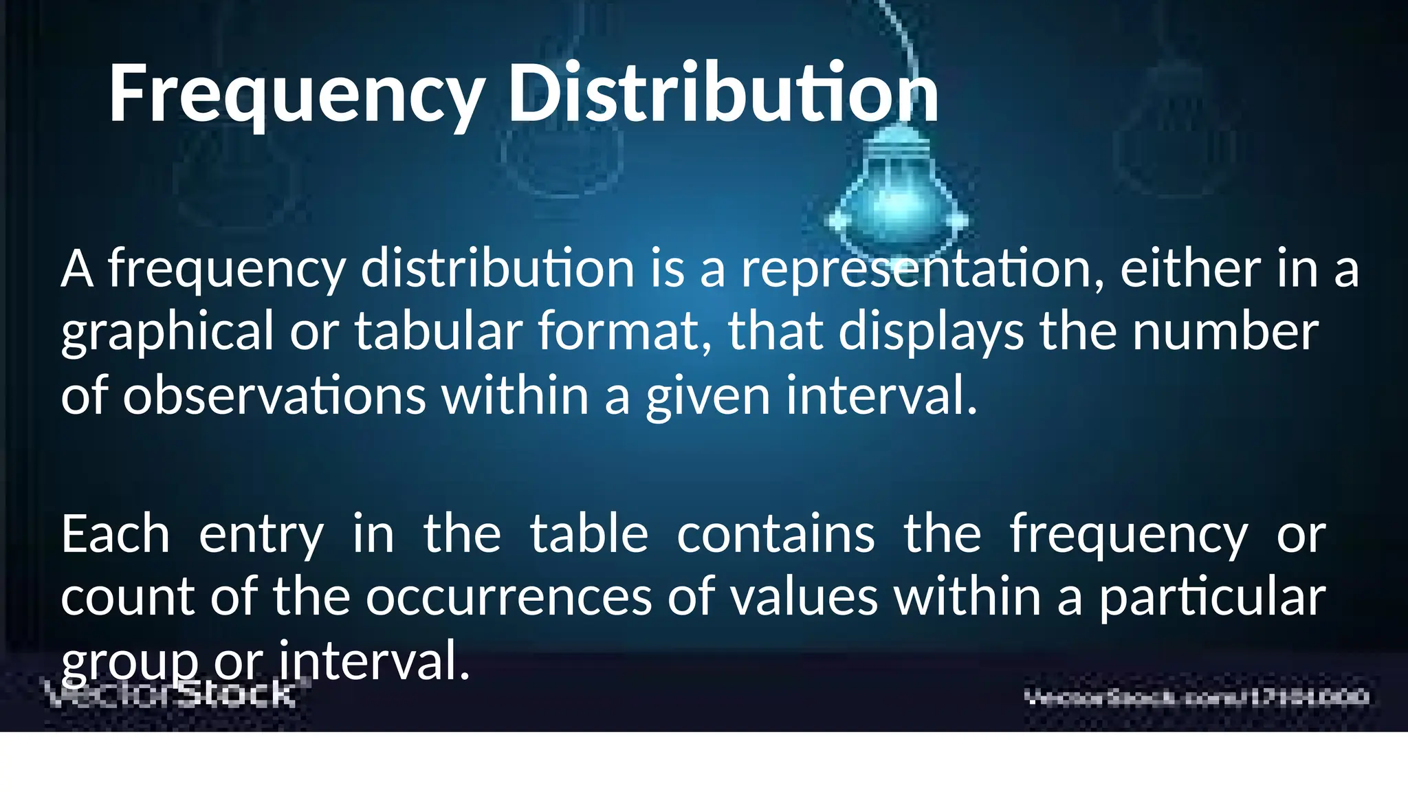
Frequency Distribution
A frequency distribution is a representation, either in a
graphical or tabular format, that displays the number
of observations within a given interval.
Each entry in the table contains the frequency or
count of the occurrences of values within a particular
group or interval.

Distribution
Examples of Frequency

?
No. of classes:
9.
-
. The class interval between 0 and 9 is defined as 0
CLASS INTERVAL
varying in a wide range. Each of these groups is defined by an interval called
Number of ‘classified groups’ from a large number of observations
:
CLASSES
•
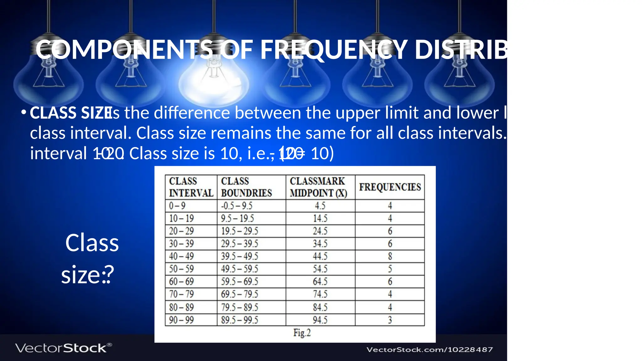
COMPONENTS OF FREQUENCY DISTRIBUTION

?
size:
Class
= 10)
10
-
. Class size is 10, i.e., (20
20
-
interval 10
class interval. Class size remains the same for all class intervals. For the class
Is the difference between the upper limit and lower limit of a
:
CLASS SIZE
•

interval is called class frequency of that class interval.
The number of observation falling within a class
:
CLASS FREQUENCY
•
2
lower limit + Upper limit)/
(
Mid value of each class =
•
interval. It is also known as the mid value.
the class
of
(Also called as class limit) is the midmost value
:
CLASS MARK
•

CLASS WIDTH refers to the difference
between the upper and lower
boundaries of any class (category).
Depending on the author, it’s also
sometimes used more specifically to mean:
• The difference between the upper limits
of two consecutive (neighboring) classes,
or
• The difference between the lower limits
of two consecutive classes.
Class width:

Note that these are different than the difference between the
upper and lower limits of a class. ?

previous class.
question and the upper limit of the
average of the lower limit of the class in
boundary of a class is defined as the
the classes or the dataset. The lower class
which separate classes. They are not part of
are the data values
CLASS BOUNDARIES
DISTRIBUTION
COMPONENTS OF FREQUENCY

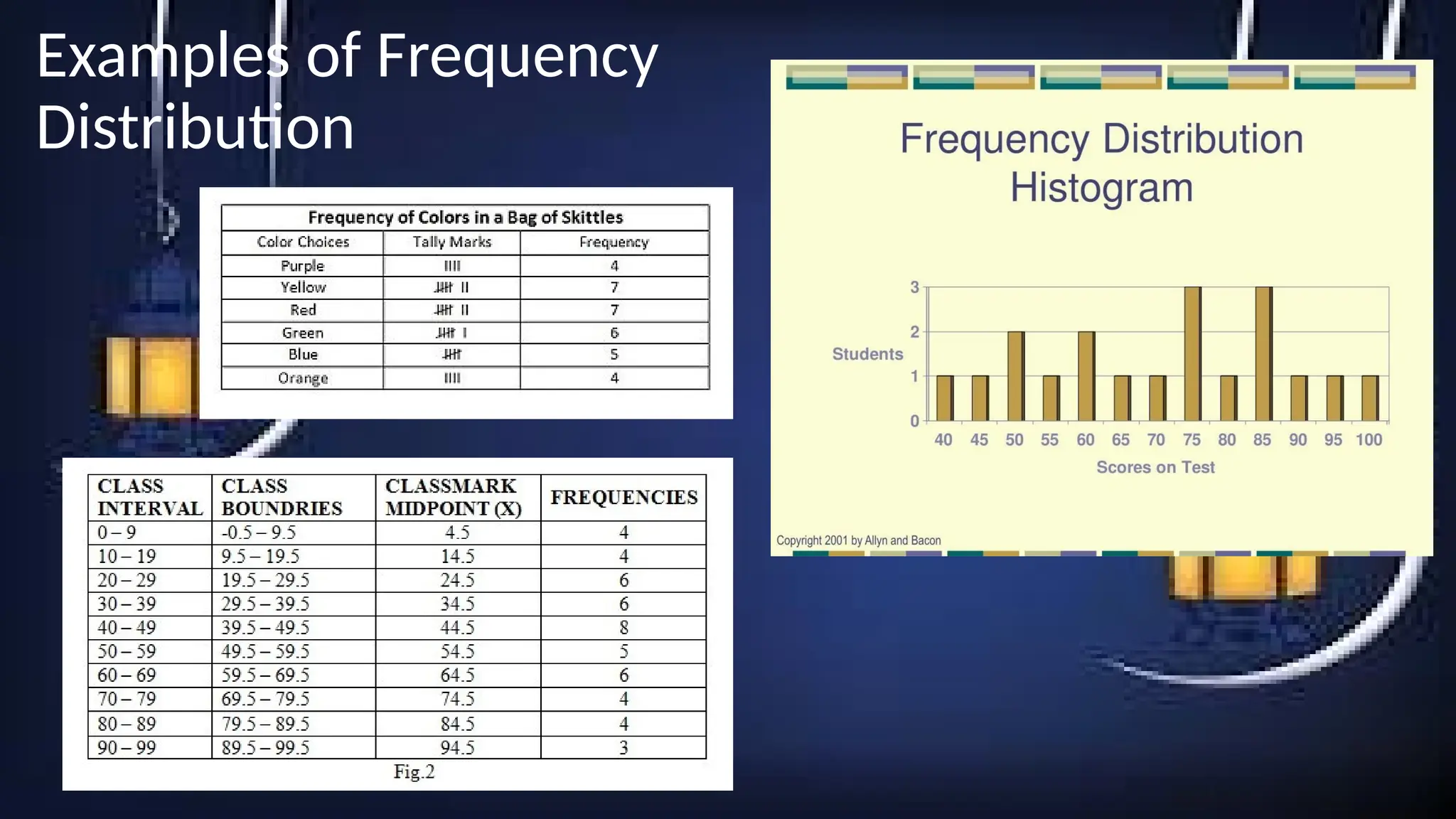
The CUMULATIVE FREQUENCY is
calculated by adding each
frequency from a frequency
distribution table to the sum of
its predecessors. The last value
will always be equal to the total
for all observations, since all
frequencies will already have
been added to the previous total.
TOTAL : 50
CLASS
INTERVAL
CLASS
BOUNDARIES
CLASS
MIDPOINT
(X)
FREQUENCIES CUMULATIVE
FREQUENCIES
0-9 -0.5 – 9.5 4.5 4 4
10-19 9.5 – 19.5 14.5 4 8
20-29 19.5 – 29.5 24.5 6 14
30-39 29.5 – 39.5 34.5 6 20
40-49 39.5 – 49.5 44.5 8 28
50-59 49.5 – 59.5 54.5 5 33
60-69 59.5 – 69.5 64.5 6 39
70-79 69.5 – 79.5 74.5 4 43
80-89 79.5 – 89.5 84.5 4 47
90-99 89.5 – 99.5 94.5 3 50

be grouped data.
in different classes then it is said to
When raw data have been grouped
bundled together in categories.
is data that has been
Grouped data
•
numbers.
set of data is basically a list of
otherwise grouped. An ungrouped
sorted into categories, classified, or
that is, it’s not
—
The data is raw
gather from an experiment or study.
is the data you first
Ungrouped data
•
Grouped and Ungrouped Data

STEPS IN CONSTRUCTING A GROUPED FREQUENCY DISTRIBUTION
Step 1 Determine the classes.
• Find the highest and lowest value.
• Find the range.
• Select the number of classes desired.
• Find the width by dividing the range by the number of classes
and rounding up.
• Select a starting point (usually the lower value); Add the
width to get the lower limits.
• Find the upper class limits.
• Find the boundaries.
Step 2 Tally the data.
Step 3 Find the numerical frequencies from the tallies.

Step 4 Find the cumulative frequencies.
https://www.youtube.com/watch?v=tcU_hApd-j0&feature=emb_logo
THINGS TO REMEMBER WHEN CONSTRUCTING
GROUPED FREQUENCY DISTRIBUTION
1.There should be between 5 to 20 classes.
2. It is preferable, but not absolutely necessary, that the class
width be an odd number.
3. The classes must be mutually exclusive (non-overlapping).
4. The classes must be continuous.
5. The classes must be exhaustive.

6. The classes must be equal in width.

Measures of Central Tendency
In statistics, a central tendency (or measure of
central tendency) is a central or typical value
for a probability distribution. It may also be
called a center or location of the distribution.
Colloquially, measures of central tendency are
often called averages. The term central
tendency dates from the late 1920s. Wikipedia

MEAN
The mean or the average is the commonly used statistic to
measure the center of a data set. It is determined by adding all
values in the data set divided by the number of values in the data
set.
Properties of Mean
⮚ It is simple to calculate.
⮚ It is the most reliable among all measures of central tendency.
⮚ It is determined by adding all values of the data divided by the sum of all values.
⮚ It is easily affected by the magnitude of (extremely high or low) scores.
⮚ The sum of each score’s deviation from the mean is zero.
⮚ It is used to compute other statistics such as standard deviation, variance, t-ratio, critical
ratio, coefficient of variation, and skewness.

⮚ It can be applied to interval and continuous data but cannot be used for nominal or
categorical data.

MEDIAN
Median is a point in a scale that divides it into two equal parts. A
scale is a succession of numbers, classes, degrees, gradations, or
categories with a fixed interval (Calderon, 2006).
Properties of Median
⮚ It is the exact midpoint of the score distribution.
⮚It is a stable measure of central tendency that is not affected by extreme values.
⮚It is used to determine whether the data values fall into the upper half or lower
half of the distribution.
⮚ It is robust to skewness and outliers.

MEDIANS OF GROUPED AND UNGROUPED DATA

MODE
The mode is the most frequently observed value in a set of data. It is the
score that occurred the most number of times, therefore with the highest
frequency. If there is only one mode in a distribution of scores, it is
unimodal. If it consists of two modes, it is called bimodal. If there are three
or more modes in a distribution, it is either called trimodal or multimodal.
Properties of Mode
⮚It is the most probable and/or typical value.
⮚The value of mode is based on the predominant frequency and not by value in the
distribution.
⮚It is unstable and influenced by grouping procedures.
Mode for Ungrouped Data

To easily find the mode for ungrouped data, sort the scores (from least to greatest or
greatest to least) and count the number times each score appears. The score that appears
the most is the mode.

percentile.
or
,
decile
,
quartile
It can be a
certain limit.
scores in a distribution are above or below a
determines how many
into equal groups. It
are cut points that divide a dataset
Quantiles
•
QUANTILES

)
points each
(5
Work within the time limit given. (30 Minutes)
•
Answer the worksheet.
•
PRACTICE EXERCISES:

directions (Frost, 2020).
mean taper off equally in both
for values further away from the
central peak and the probabilities
observations cluster around the
distribution where most of the
distribution is a symmetric
the “bell curve.” The normal
around the central values and form
likewise cases that data tend to be
left (negatively skewed). There are
positively skewed) or more on the
(
out either more on the right
Data can be distributed or spread
Normal Distribution
)
BELL CURVE
(
DISTRIBUTION
The NORMAL

less than the median.
above the mean. The mean value is
that most of the students’ scores are
sk < 0. The shape of the data implies
end tail is the left of the curve. The
negatively skewed when the thinner
On the other hand, the distribution is
mean.
consequently achieved scores lower than the
they performed poorly in the test and
students either found the test to be difficult or
lower than the mean. This happens when the
median which means that most of the scores are
distribution, the mean value is higher than the
to the right part of the curve. The sk > 0. In this
the right where the longer or flatter end tail goes
The positively skewed distribution is skewed to

5.
17.50, and sd=
=
a reading test with the following given values: mean value= 15.35, median value
Example: Find the coefficient of skewness of 20 scores of the students who took
•

How do we interpret the value of skewness?

Standard Scores
Teachers can come up with further and more meaningful
analysis and interpretation of students’ performance. To realize this,
they can make use of the actual or raw scores that are based on the
number of items that were answered correctly by the students.
Another way of doing this is by transforming or converting the raw
scores to standard scores.

The fundamental standard scores include the z-scores, t-scores,
stanines, and percentile ranks.

takers in a test.
-
all test
relative to the performance of
performance of a student
number that will represent the
it can be used to assign a
score,
-
score and T
-
Similar to z
the reference group.
ability) relative to the norm of
to 9 (indicating very superior
(indicating very poor ability)
1
point scale ranging from
-
a nine
way to rescale raw scores using
is a
Stanine or standard nine
Stanine

.
university
the
in
enroll
to
accommodated
be
can’t
he
hence,
;
university
the
by
set
6
stanine
of
rating
off
-
cut
the
obtain
to
failed
He
.
average
as
interpreted
5
of
score
stanine
given
a
with
129
and
99
between
comes
that
125
is
score
Andrew’s
.
5
stanine
assigned
are
)
129
-
99
scores
raw
(
scores
ranked
%
20
next
The
.
6
stanine
assigned
are
)
153
-
134
scores
raw
(
scores
ranked
%
17
next
The
.
7
stanine
assigned
are
)
167
-
154
scores
raw
(
scores
ranked
%
12
next
The
.
8
stanine
assigned
are
)
174
-
168
scores
raw
(
scores
ranked
%
7
next
The
.
9
stanine
assigned
are
)
187
-
186
scores
raw
(
scores
ranked
%
4
first
The
:
Solution

Interpretation and Utilization of Assessment Results.docx

More Related Content

Similar to Interpretation and Utilization of Assessment Results.docx

Recently uploaded

Interpretation and Utilization of Assessment Results.docx