Greedy Algorithms Chapter for new students 4.ppt

Greedy Algorithms
Greedy Algorithms
Chapter 4

2
Greedy Technique
Greedy Technique
Constructs a solution to an
Constructs a solution to an optimization problem
optimization problem piece by
piece by
piece through a sequence of choices that are:
piece through a sequence of choices that are:
 feasible
feasible
 locally optimal
locally optimal
 irrevocable
irrevocable
For some problems, yields an optimal solution for every instance.
For some problems, yields an optimal solution for every instance.
For most, does not but can be useful for fast approximations.
For most, does not but can be useful for fast approximations.

3
Applications of the Greedy Strategy
Applications of the Greedy Strategy
 Optimal solutions:
Optimal solutions:
• change making for “normal” coin denominations
change making for “normal” coin denominations
• minimum spanning tree (MST)
minimum spanning tree (MST)
• single-source shortest paths
single-source shortest paths
• simple scheduling problems
simple scheduling problems
• Huffman codes
Huffman codes
 Approximations:
Approximations:
• traveling salesman problem (TSP)
traveling salesman problem (TSP)
• knapsack problem
knapsack problem
• other combinatorial optimization problems
other combinatorial optimization problems

4
Change-Making Problem
Given unlimited amounts of coins of denominations
Given unlimited amounts of coins of denominations d
d1
1 > … >
> … > d
dm
m ,
,
give change for amount
give change for amount n
n with the least number of coins
with the least number of coins
Example:
Example: d
d1
1 = 25c,
= 25c, d
d2
2 =10c,
=10c, d
d3
3 = 5c,
= 5c, d
d4
4 = 1c and
= 1c and n =
n = 48c
48c
Greedy solution:
Greedy solution:
Greedy solution:
Greedy solution:
 optimal for any amount and “typical’’ set of denominations
optimal for any amount and “typical’’ set of denominations
 not optimal for all coin denominations …
not optimal for all coin denominations …

5
Greedy not optimal for all sets of denominations:
Greedy not optimal for all sets of denominations:
 Consider 1, 3, 4
Consider 1, 3, 4
 For what value does greedy algorithm fail?
For what value does greedy algorithm fail?

6
Minimum Spanning Tree (MST)
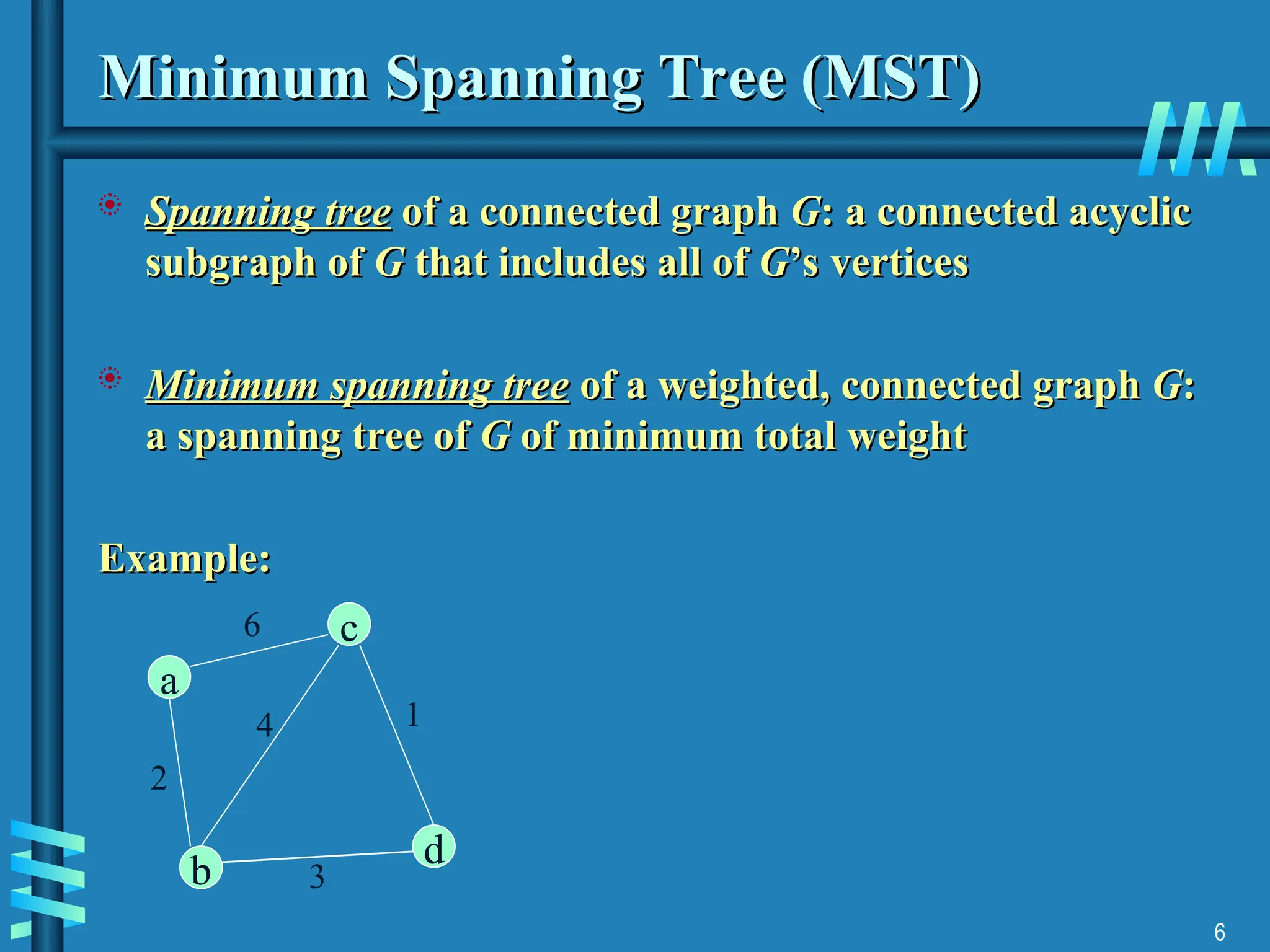
Minimum Spanning Tree (MST)
 Spanning tree
Spanning tree of a connected graph
of a connected graph G
G: a connected acyclic
: a connected acyclic
subgraph of
subgraph of G
G that includes all of
that includes all of G
G’s vertices
’s vertices
 Minimum spanning tree
Minimum spanning tree of a weighted, connected graph
of a weighted, connected graph G
G:
:
a spanning tree of
a spanning tree of G
G of minimum total weight
of minimum total weight
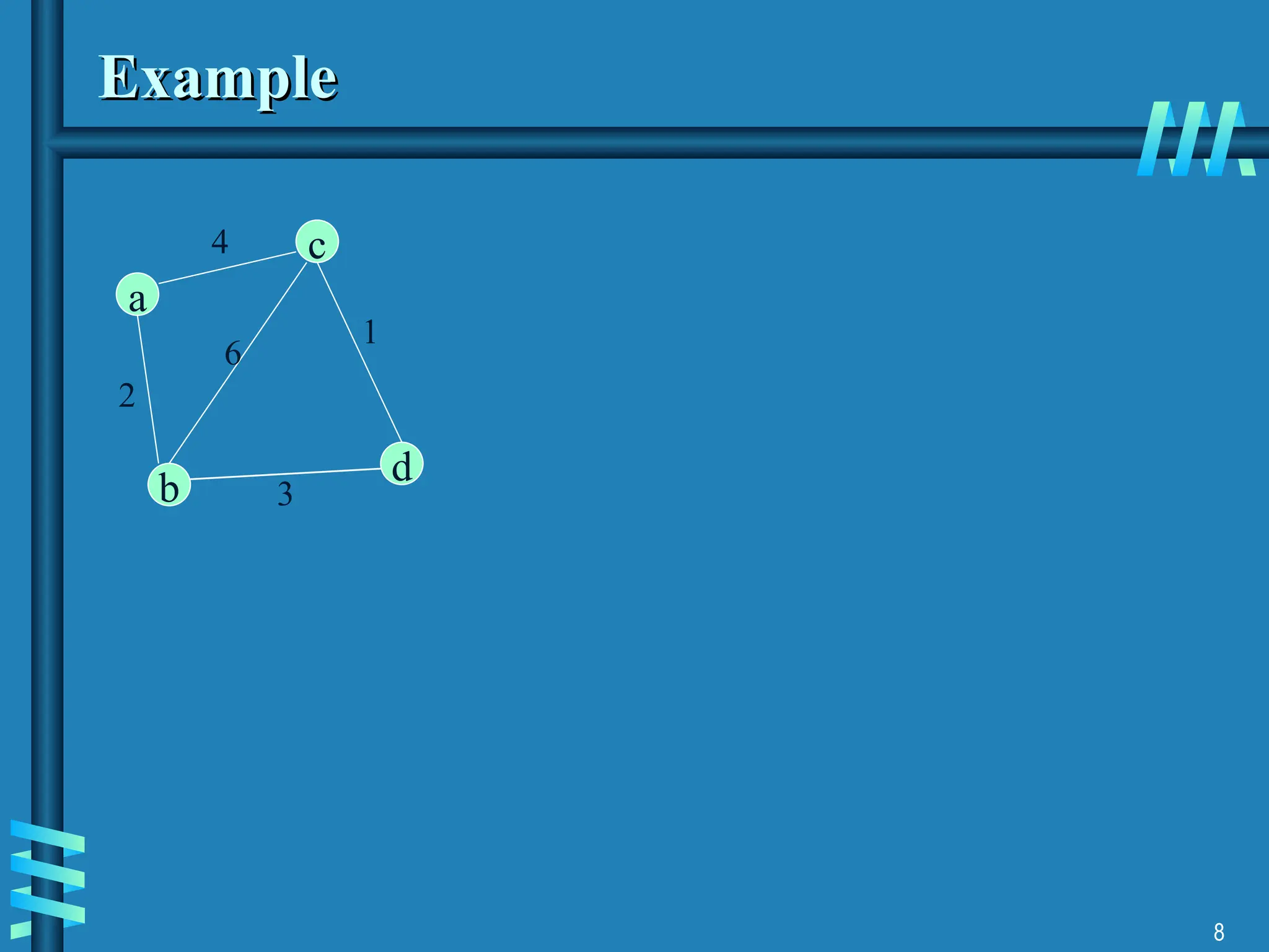
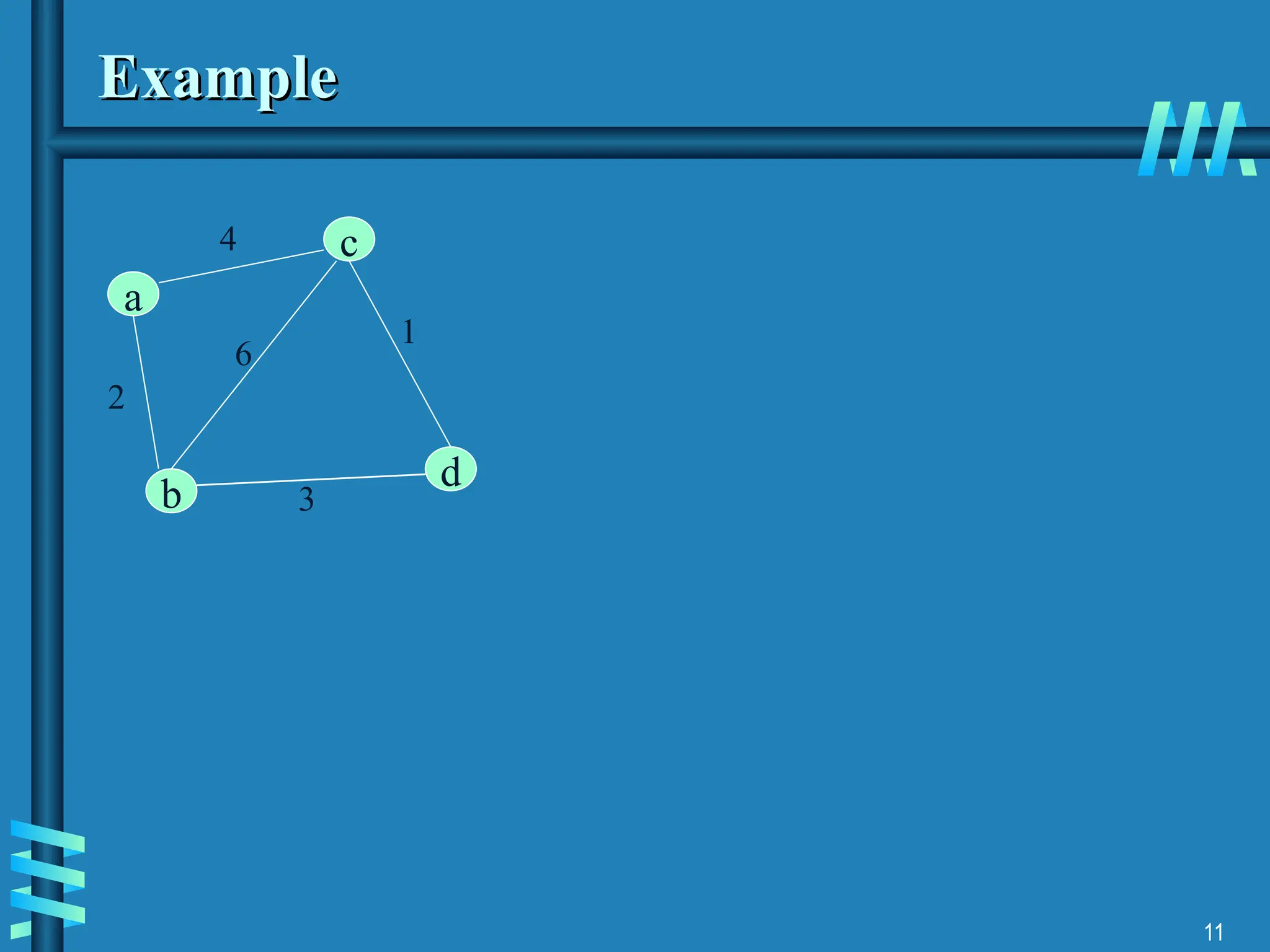
Example:
Example:
c
d
b
a
6
2
4
3
1

7
Prim’s MST algorithm
Prim’s MST algorithm
 Start with tree
Start with tree T
T1
1 consisting of one (any) vertex and “grow”
consisting of one (any) vertex and “grow”
tree one vertex at a time to produce MST through
tree one vertex at a time to produce MST through a series of
a series of
expanding subtrees T
expanding subtrees T1
1, T
, T2
2, …, T
, …, Tn
n
 On each iteration,
On each iteration, construct T
construct Ti
i+1
+1 from T
from Ti
i by adding vertex
by adding vertex
not in
not in T
Ti
i that is
that is closest to those already in
closest to those already in T
Ti
i (this is a
(this is a
“greedy” step!)
“greedy” step!)
 Stop when all vertices are included
Stop when all vertices are included

8
Example
Example
c
d
b
a
4
2
6
1
3

9
Notes about Prim’s algorithm
Notes about Prim’s algorithm
 Proof by induction that this construction actually yields MST
Proof by induction that this construction actually yields MST
 Needs priority queue for locating closest fringe vertex
Needs priority queue for locating closest fringe vertex
 Efficiency
Efficiency
• O(
O(n
n2
2
)
) for weight matrix representation of graph and array
for weight matrix representation of graph and array
implementation of priority queue
implementation of priority queue
• O
O(
(m
m log
log n
n) for adjacency list representation of graph with
) for adjacency list representation of graph with
n
n vertices and
vertices and m
m edges and min-heap implementation of
edges and min-heap implementation of
priority queue
priority queue

10
Another greedy algorithm for MST: Kruskal’s
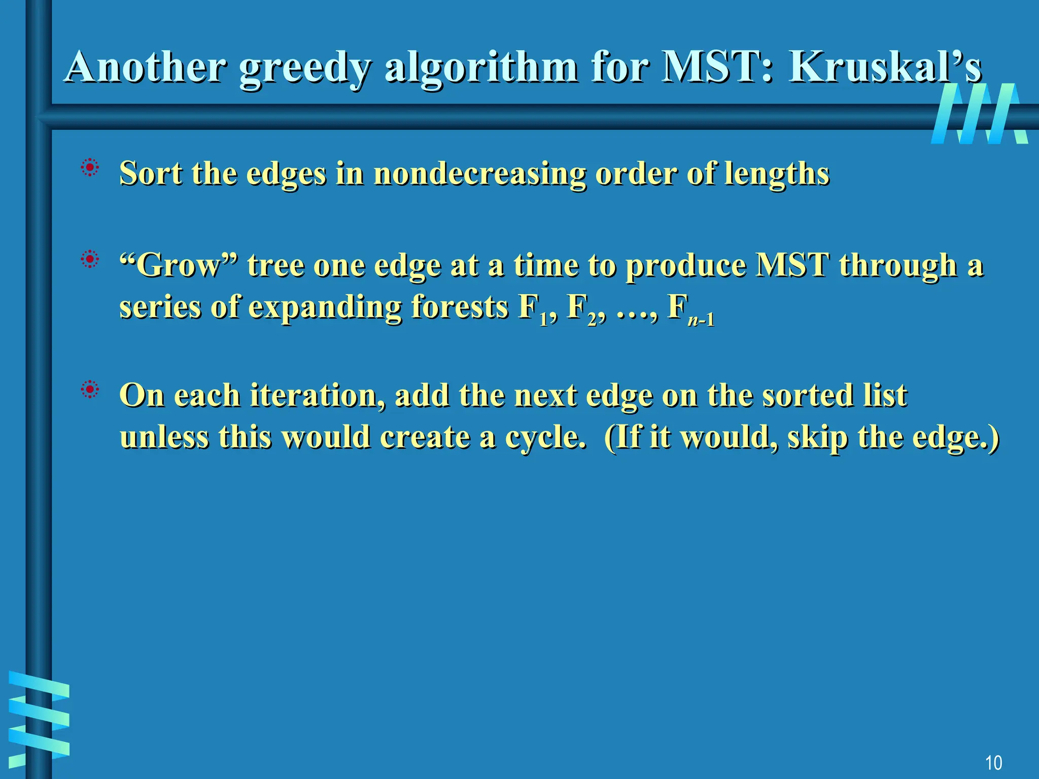
Another greedy algorithm for MST: Kruskal’s
 Sort the edges in nondecreasing order of lengths
Sort the edges in nondecreasing order of lengths
 “
“Grow” tree one edge at a time to produce MST through
Grow” tree one edge at a time to produce MST through a
a
series of expanding forests F
series of expanding forests F1
1, F
, F2
2, …, F
, …, Fn-
n-1
1
 On each iteration, add the next edge on the sorted list
On each iteration, add the next edge on the sorted list
unless this would create a cycle. (If it would, skip the edge.)
unless this would create a cycle. (If it would, skip the edge.)

11
Example
Example
c
d
b
a
4
2
6
1
3

12
Notes about Kruskal’s algorithm
Notes about Kruskal’s algorithm
 Algorithm looks easier than Prim’s but is harder to
Algorithm looks easier than Prim’s but is harder to
implement (checking for cycles!)
implement (checking for cycles!)
 Cycle checking: a cycle is created iff added edge connects
Cycle checking: a cycle is created iff added edge connects
vertices in the same connected component
vertices in the same connected component
 Union-find
Union-find algorithms – see section 9.2
algorithms – see section 9.2

13
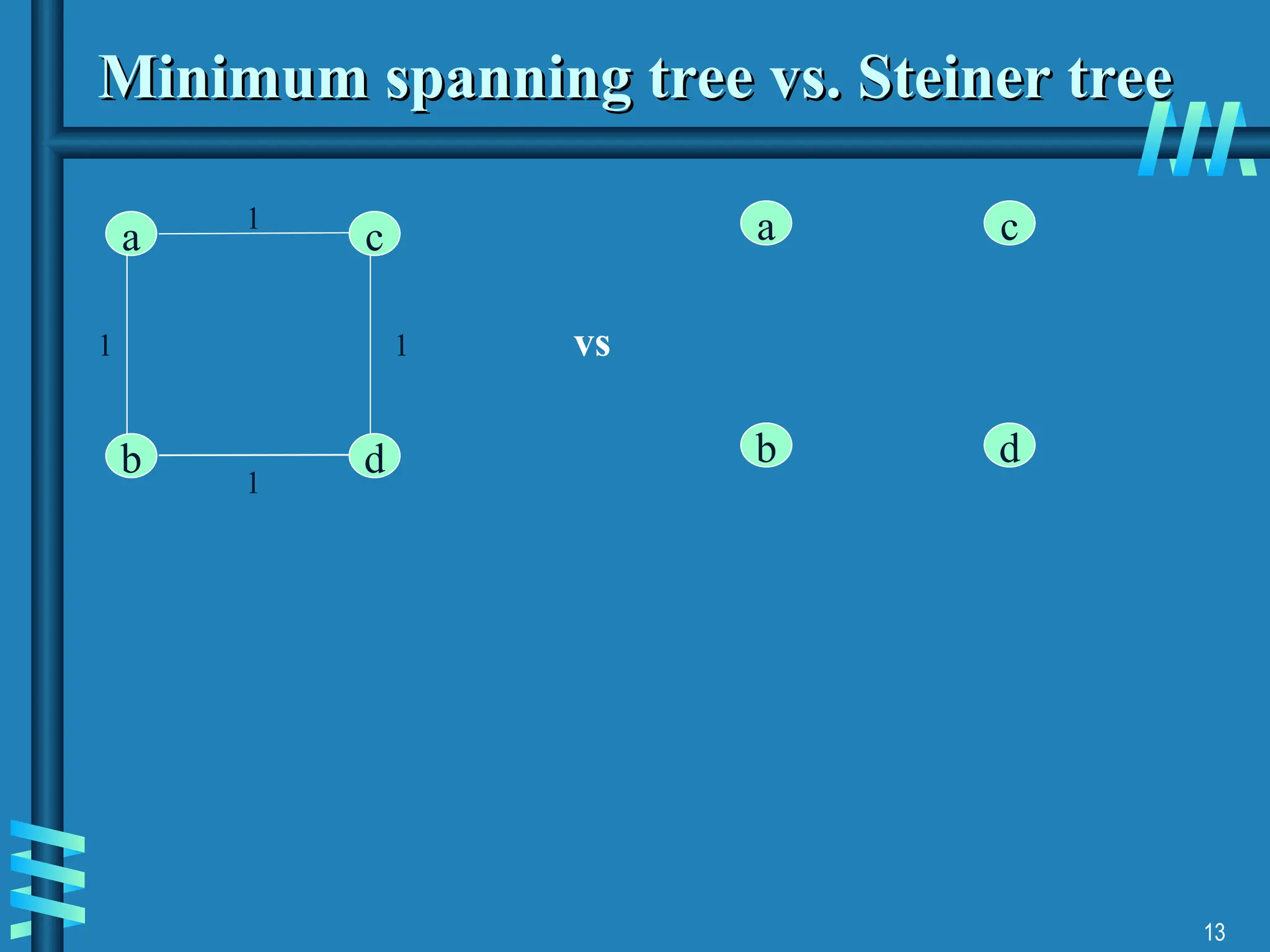
Minimum spanning tree vs. Steiner tree
Minimum spanning tree vs. Steiner tree
c
d
b
a
1
1 1
1
c
d
b
a
vs

14
Shortest paths – Dijkstra’s algorithm
Shortest paths – Dijkstra’s algorithm
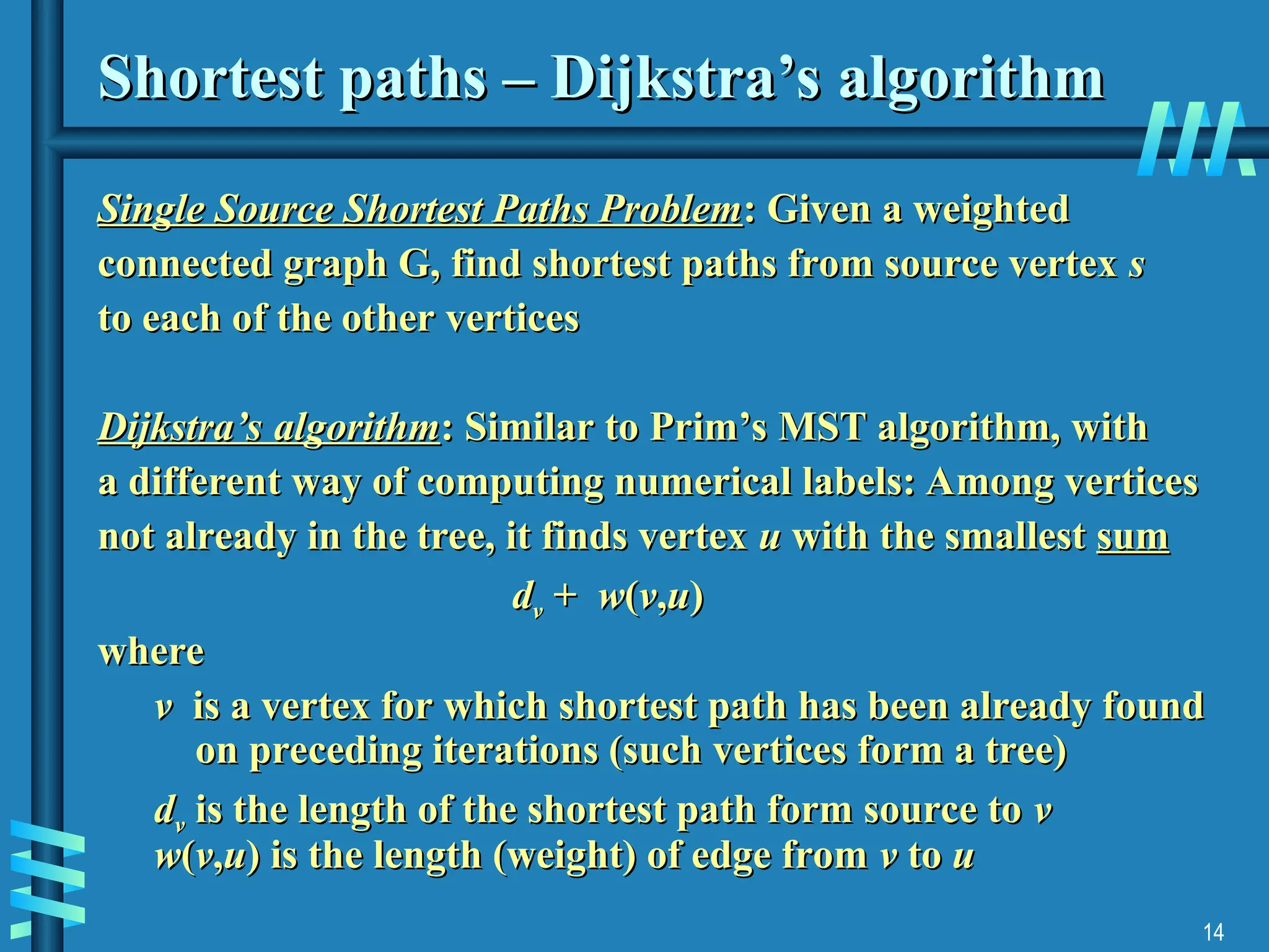
Single Source Shortest Paths Problem
Single Source Shortest Paths Problem: Given a weighted
: Given a weighted
connected graph G, find shortest paths from source vertex
connected graph G, find shortest paths from source vertex s
s
to each of the other vertices
to each of the other vertices
Dijkstra’s algorithm
Dijkstra’s algorithm: Similar to Prim’s MST algorithm, with
: Similar to Prim’s MST algorithm, with
a different way of computing numerical labels: Among vertices
a different way of computing numerical labels: Among vertices
not already in the tree, it finds vertex
not already in the tree, it finds vertex u
u with the smallest
with the smallest sum
sum
d
dv
v +
+ w
w(
(v
v,
,u
u)
)
where
where
v
v is a vertex for which shortest path has been already found
is a vertex for which shortest path has been already found
on preceding iterations (such vertices form a tree)
on preceding iterations (such vertices form a tree)
d
dv
v is the length of the shortest path form source to
is the length of the shortest path form source to v
v
w
w(
(v
v,
,u
u) is the length (weight) of edge from
) is the length (weight) of edge from v
v to
to u
u

15
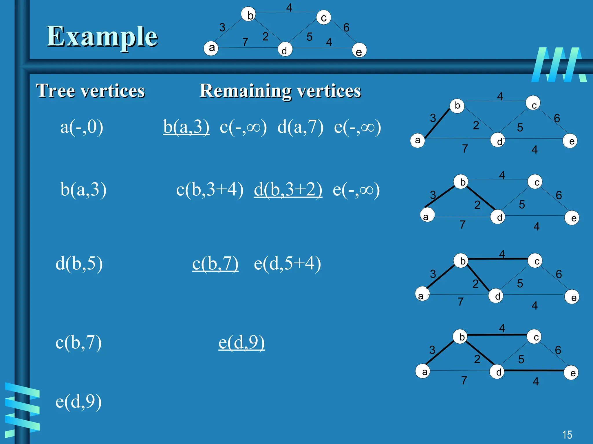
Example
Example d
4
Tree vertices Remaining vertices
Tree vertices Remaining vertices
a(-,0) b(a,3) c(-,∞) d(a,7) e(-,∞)
a
b
4
e
3
7
6
2 5
c
a
b
d
4
c
e
3
7 4
6
2 5
a
b
d
4
c
e
3
7 4
6
2 5
a
b
d
4
c
e
3
7 4
6
2 5
b(a,3) c(b,3+4) d(b,3+2) e(-,∞)
d(b,5) c(b,7) e(d,5+4)
c(b,7) e(d,9)
e(d,9)
d
a
b
d
4
c
e
3
7 4
6
2 5

16
Notes on Dijkstra’s algorithm
Notes on Dijkstra’s algorithm
 Doesn’t work for graphs with negative weights
Doesn’t work for graphs with negative weights
 Applicable to both undirected and directed graphs
Applicable to both undirected and directed graphs
 Efficiency
Efficiency
• O(|V|
O(|V|2
2
) for graphs represented by weight matrix and
) for graphs represented by weight matrix and
array implementation of priority queue
array implementation of priority queue
• O(|E|log|V|) for graphs represented by adj. lists and
O(|E|log|V|) for graphs represented by adj. lists and
min-heap implementation of priority queue
min-heap implementation of priority queue
 Don’t mix up Dijkstra’s algorithm with Prim’s algorithm!
Don’t mix up Dijkstra’s algorithm with Prim’s algorithm!

17
Coding Problem
Coding Problem
Coding
Coding: assignment of bit strings to alphabet characters
: assignment of bit strings to alphabet characters
Codewords
Codewords: bit strings assigned for characters of alphabet
: bit strings assigned for characters of alphabet
Two types of codes:
Two types of codes:
 fixed-length encoding
fixed-length encoding (e.g., ASCII)
(e.g., ASCII)
 variable-length encoding
variable-length encoding (e,g., Morse code)
(e,g., Morse code)
Prefix-free codes
Prefix-free codes: no codeword is a prefix of another codeword
: no codeword is a prefix of another codeword
Problem: If frequencies of the character occurrences are
Problem: If frequencies of the character occurrences are
known, what is the best binary prefix-free code?
known, what is the best binary prefix-free code?

18
Huffman codes
Huffman codes
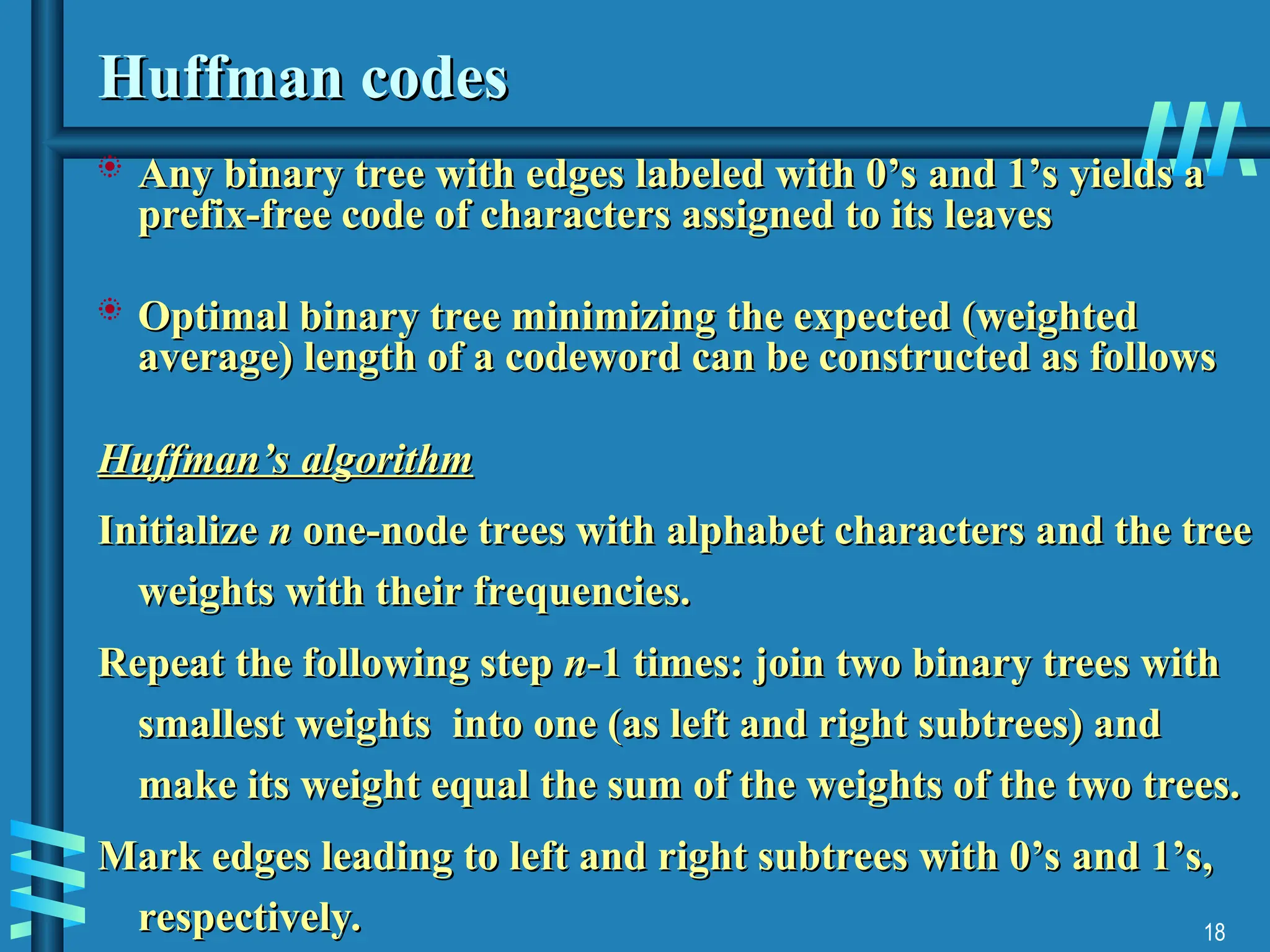
 Any binary tree with edges labeled with 0’s and 1’s yields a
Any binary tree with edges labeled with 0’s and 1’s yields a
prefix-free code of characters assigned to its leaves
prefix-free code of characters assigned to its leaves
 Optimal binary tree minimizing the expected (weighted
Optimal binary tree minimizing the expected (weighted
average) length of a codeword can be constructed as follows
average) length of a codeword can be constructed as follows
Huffman’s algorithm
Huffman’s algorithm
Initialize
Initialize n
n one-node trees with alphabet characters and the tree
one-node trees with alphabet characters and the tree
weights with their frequencies.
weights with their frequencies.
Repeat the following step
Repeat the following step n
n-1 times: join two binary trees with
-1 times: join two binary trees with
smallest weights into one (as left and right subtrees) and
smallest weights into one (as left and right subtrees) and
make its weight equal the sum of the weights of the two trees.
make its weight equal the sum of the weights of the two trees.
Mark edges leading to left and right subtrees with 0’s and 1’s,
Mark edges leading to left and right subtrees with 0’s and 1’s,
respectively.
respectively.

19
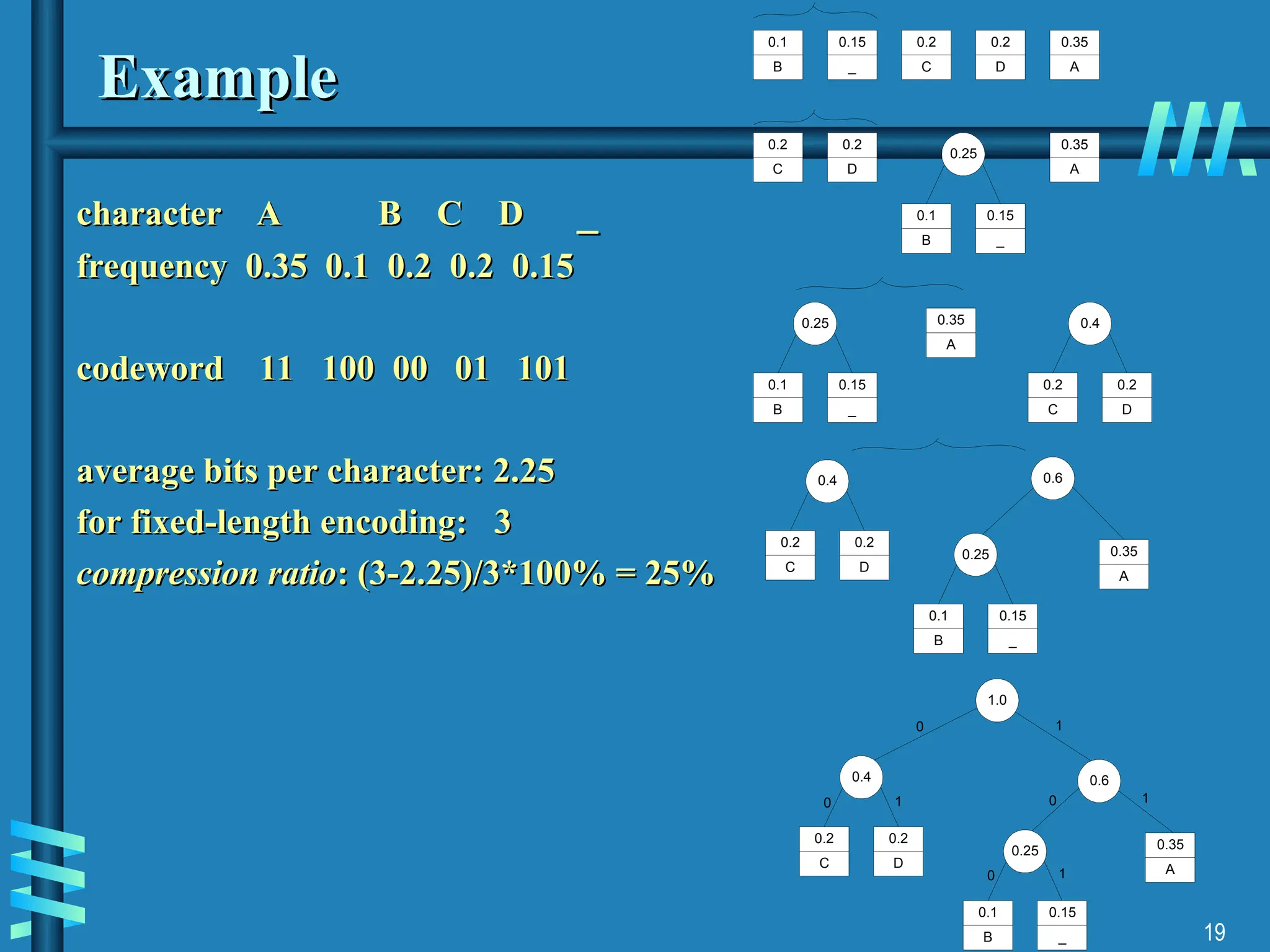
Example
Example
character A
character A B C D
B C D _
_
frequency 0.35 0.1 0.2 0.2 0.15
frequency 0.35 0.1 0.2 0.2 0.15
codeword 11 100 00 01 101
codeword 11 100 00 01 101
average bits per character: 2.25
average bits per character: 2.25
for fixed-length encoding: 3
for fixed-length encoding: 3
compression ratio
compression ratio: (3-2.25)/3*100% = 25%
: (3-2.25)/3*100% = 25%
0.25
0.1
B
0.15
_
0.2
C
0.2
D
0.35
A
0.2
C
0.2
D
0.35
A
0.1
B
0.15
_
0.4
0.2
C
0.2
D
0.6
0.25
0.1
B
0.15
_
0.6
1.0
0 1
0.4
0.2
C
0.2
D
0.25
0.1
B
0.15
_
0 1 0
0
1
1
0.25
0.1
B
0.15
_
0.35
A
0.4
0.2
C
0.2
D
0.35
A
0.35
A

Greedy Algorithms Chapter for new students 4.ppt

More Related Content

Similar to Greedy Algorithms Chapter for new students 4.ppt

More from AKBARABBAS11

Recently uploaded

Greedy Algorithms Chapter for new students 4.ppt